Topological effects in continuum 2d $U(N)$ gauge theories

Abstract

We study the $\theta$ dependence of the continuum limit of 2d $U(N)$ gauge theories defined on compact manifolds, with special emphasis on spherical ($g=0$) and toroidal ($g=1$) topologies. We find that the coupling between $U(1)$ and $SU(N)$ degrees of freedom survives the continuum limit, leading to observable deviations of the continuum topological susceptibility from the $U(1)$ behavior, especially for $g=0$, in which case deviations remain even in the large $N$ limit.

I Introduction

It is well known that two dimensional gauge theories are analytically much more tractable than their four dimensional counterparts, and in some cases some exact nonperturbative expressions can even be obtained. Quite surprisingly, however, the $\theta$ dependence of these two dimensional models appears not to have been investigated until very recently.

In the paper Bonati:2019ylr we filled this gap, by presenting analytic results for various aspects of the $\theta$ dependence of two dimensional $U(N)$ gauge theories. By generalizing the argument presented in Rusakov:1990rs (see also Witten:1991we ; Kiskis:2014lwa for different approaches), the partition function at $\theta\neq 0$ of the lattice $U(N)$ gauge theory (with Wilson action) was written as sum over the representations of $U(N)$ of some character’s related coefficients. This expression, although exact, is of little practical use due to its complexity, so some limit cases were also investigated: the continuum limit at finite area $A$, the thermodynamic limit $A\to\infty$ and the large $N$ limit in the thermodynamic case (i.e. at $A=\infty$).

The two main outcomes of this analysis were the following: the first one is that, in the thermodynamic limit, the large $N$ behaviour of the topological susceptibility is different in the weak and strong coupling phases identified by the Gross-Witten-Wadia transition Gross:1980he ; Wadia:1980cp . Indeed for ’t Hooft coupling $\beta<1/2$ the susceptibility diverges in the large $N$ limit, while for $\beta>1/2$ its value is related to the expectation value of the determinant of the link variables, as computed in Rossi:1982vw . The second noteworthy result is a rather unexpected feature of the continuum limit: against naive expectations based on continuum intuition, $SU(N)$ and $U(1)$ degrees of freedom do not decouple from each other even in the continuum limit as far as $A<\infty$.

In this paper we will elaborate more on the second point, by rewriting the continuum partition function in a form that makes manifest the interaction of the $SU(N)$ degrees of freedom with the instanton sectors of the $U(1)$ theory. We will also discuss the large $N$ limit at finite area and, in the case of spherical topology ($g=0$), we will present numerical evidence that the topological susceptibility behaves as an order parameter for the Douglas-Kazakov transition Douglas:1993iia .

II The partition function in the continuum limit

In Bonati:2019ylr it was shown that, starting from the Wilson action and the discretization

$$q(U_{p})=-\frac{i}{2\pi}\mathrm{Tr}\ln U_{p}\ ,$$ (1)

of the topological charge density ($U_{p}$ is the parallel transporter around a plaquette), the $\theta$ dependent, finite area partition function of the continuum $U(N)$ model can be written in the form

$$Z_{\theta}^{(g)}(N,X)=\sum_{\{l_{j}\}}d_{\{l_{j}\}}^{2-2g}e^{-{X\over 2N}\big{[}C_{\{l_{j}\}}+{\theta\over\pi}\sum_{j}l_{j}+{N\over 4\pi^{2}}\theta^{2}\big{]}}\ .$$ (2)

Here the $N$ integer numbers $\{l_{j}\}$ (with $l_{1}\geq l_{2}\geq\cdots\geq l_{N}$) label the representations of $U(N)$ (see e.g. Drouffe:1983fv ), $g$ is the genus of the manifold on which the theory is defined and $X=A/2\beta$ is a dimensionless variable, depending on the area $A$ of the manifold and on the ’t Hooft coupling $\beta$. $d_{\{l_{j}\}}$ and $C_{\{l_{j}\}}$ denote the dimension and the quadratic Casimir of the representation identified by $\{l_{j}\}$, whose explicit expressions are

$$C_{\{l_{j}\}} =\sum_{j=1}^{N}l_{j}(l_{j}-2j+N+1)=$$ (3)

$$=\sum_{j=1}^{N}\left(l_{j}-j+\frac{N+1}{2}\right)^{2}-\frac{N(N^{2}-1)}{12}\ ,$$

$$d_{\{l_{j}\}} =\prod_{k>j}\left(1-\frac{l_{k}-l_{j}}{k-j}\right)\ .$$

It is important to note that the expression in Eq. (2) is consistent with the periodicity in $\theta$ of the partition function, with period $2\pi$. Indeed the exponents appearing in Eq. (2) can be rewritten in the form

$$C_{\{l_{j}\}}+\frac{\theta}{\pi}\sum_{j}l_{j}+\frac{N}{4\pi^{2}}\theta^{2}=$$ (4)

$$=\sum_{j=1}^{N}\left(l_{j}+\frac{\theta}{2\pi}-j+\frac{N+1}{2}\right)^{2}-\frac{N(N^{2}-1)}{12}\ ;$$

as a consequence $\theta\to\theta+2\pi$ is equivalent to $\{l_{j}\}\to\{l^{\prime}_{j}\}$ where $l^{\prime}_{j}=l_{j}+1$. Since $d_{\{l^{\prime}_{j}\}}=d_{\{l_{j}\}}$ the $2\pi-$periodicity of Eq. (2) immediately follows.

The particular case of the $U(1)$ gauge theory is obviously the simplest one: in this case the partition function does not depend on the genus $g$ of the manifold and it is simply given by

$$Z_{\theta}(1,X)=\sum_{n}e^{-\frac{X}{2}\left(n+\frac{\theta}{2\pi}\right)^{2}}\ ,$$ (5)

a result that can be readily obtained using more conventional methods (see e.g. Cao:2013na ).

The topological susceptibility $\chi_{t}^{(g)}(N,\beta,A)$ can be computed by using the general relation

$$\chi_{t}^{(g)}(N,\beta,A)=-\frac{1}{A}\frac{\partial^{2}}{\partial\theta^{2}}\log Z_{\theta}^{(g)}(N,X)$$ (6)

and, to make the notation more compact, it is convenient to define the (normalized) weights

$$w_{\{l_{j}\}}^{(g)}\big{(}N,X\big{)}=d_{\{l_{j}\}}^{2-2g}e^{-{X\over 2N}C_{\{l_{j}\}}}\Bigl{[}Z_{0}^{(g)}\big{(}N,X\big{)}\Bigr{]}^{-1}.$$ (7)

The finite volume continuum limit of the topological susceptibility (at $\theta=0$) is then given by

$$\chi_{t}^{(g)}(N,\beta,A)=\frac{1}{8\pi^{2}\beta}\Big{[}1-X\sum_{\{l_{j}\}}w_{\{l_{j}\}}^{(g)}\Big{(}\sum_{j}\frac{l_{j}}{N}\Big{)}^{2}\Big{]}\ ,$$ (8)

where the relation

$$\sum_{\{l_{j}\}}\Big{(}w_{\{l_{j}\}}^{(g)}\sum_{j}l_{j}\Big{)}=0$$ (9)

was used to simplify the result. This relation holds true since for each representation $\{l_{j}\}$ the conjugate representation $\{l^{\prime}_{j}\}$ (with $l^{\prime}_{j}=-l_{N+1-j}$) has the same weight of $\{l_{j}\}$ and $\sum_{j}l^{\prime}_{j}=-\sum_{j}l_{j}$.

In the infinite volume limit $X\to\infty$ it is easily seen that $w_{\{l_{j}\}}^{(g)}\to\delta_{\{l_{j}\},\{0\}}$ (where $\{0\}$ denotes the trivial representation), and in this limit the topological susceptibility does not depend on the genus $g$ and on the number of colors $N$, becoming simply equal to

$$\chi_{t}(N,\beta,\infty)=\frac{1}{8\pi^{2}\beta}\ .$$ (10)

Hence from now on, in order to simplify the notation, we shall express our results for the topological susceptibility in terms of the dimensionless ratio

$$R^{(g)}(N,X)\ \equiv\frac{\chi_{t}^{(g)}(N,\beta,A)}{\chi_{t}(N,\beta,\infty)}\ .$$ (11)

In some cases it will be useful to study also the derivative of $R^{(g)}(N,X)$ with respect to the area-related parameter $X$. An explicit expression for this quantity is

$${\partial R^{(g)}(N,X)\over\partial X}=\frac{X}{2N}\Bigg{[}\sum_{\{l_{j}\}}w_{\{l_{j}\}}^{(g)}C_{\{l_{j}\}}\Big{(}\sum_{j}\frac{l_{j}}{N}\Big{)}^{2}-$$ (12)

$$-\Bigg{(}\sum_{\{l_{j}\}}w_{\{l_{j}\}}^{(g)}C_{\{l_{j}\}}\Bigg{)}\Bigg{(}\sum_{\{l_{j}\}}w_{\{l_{j}\}}^{(g)}\Big{(}\sum_{j}\frac{l_{j}}{N}\Big{)}^{2}\Bigg{)}\Bigg{]}-$$

$$-\sum_{\{l_{j}\}}w_{\{l_{j}\}}^{(g)}\Big{(}\sum_{j}\frac{l_{j}}{N}\Big{)}^{2}.\$$

With the aim of clarifying the interaction between the $SU(N)$ and the $U(1)$ degrees of freedom, it is convenient to notice that representations of $U(N)$ can be unambiguously obtained from the representations of $SU(N)$ (see e.g. Drouffe:1983fv ). In order to better exploit the symmetry between representations and their conjugates we change the summation index from $j$ to $i$, by setting

$$i=j-{N+1\over 2},$$ (13)

where $j\in\{1,\ldots,N\}$ and the (integer or half-integer) numbers $i$ runs from $-{1\over 2}(N-1)$ to ${1\over 2}(N-1)$. Representations of $SU(N)$ can be labelled by the (integer or half-integer) numbers $m_{i}=l_{i}-i$, with the condition $m_{i}>m_{i+1}$ and an additional (conventional) constraint fixing the value of one of the $m_{i}$ in order to avoid double counting (we can for example fix $m_{\frac{N-1}{2}}=-\frac{N-1}{2}$, which is equivalent to the condition $l_{N}=0$ used in Drouffe:1983fv ). The representations of $U(N)$ will then be obtained from those of $SU(N)$ by the substitutions $\{m_{i}\}\rightarrow\{m_{i}+n\}$, for all $n\in\mathbb{Z}$.

To rewrite the partition function we observe that the relation between the quadratic Casimir of $U(N)$ (denoted by $C_{\{l_{j}\}}$) and the corresponding one of $SU(N)$ (denoted by $C_{\{m_{i}\}}$) is

$$C_{\{m_{i}\}}=C_{\{l_{j}\}}-\frac{1}{N}\Big{(}\sum_{j=1}^{N}l_{j}\Big{)}^{2},$$ (14)

and, since $\sum_{i}m_{i}=\sum_{j}l_{j}$, we have

$$\frac{1}{N}C_{\{m_{i}\}}=\frac{1}{N}\sum_{i}m_{i}^{2}-\Big{(}\frac{1}{N}\sum_{i}m_{i}\Big{)}^{2}-\frac{N^{2}-1}{12}\ .$$ (15)

Moreover the relation between the dimensions of the representations is

$$d_{\{m_{i}\}}=\prod_{k>i}\left(\frac{m_{i}-m_{k}}{k-i}\right)=d_{\{l_{j}\}}\ .$$ (16)

These observations allow to decompose the summation on $\{l_{j}\}$ in Eq. (2) into a summation on $\{m_{i}\}$ and a summation on $n$: it is easy to show that, by applying the above decomposition, the partition function may be expressed as

$$\hskip 85.35826ptZ_{\theta}^{(g)}(N,X)=$$ (17)

$$=\sum_{\{m_{i}\}}d^{2-2g}_{\{m_{i}\}}e^{-\frac{X}{2N}C_{\{m_{i}\}}}\sum_{n}e^{-{X\over 2}(n+{\theta\over 2\pi}+{1\over N}\sum_{i}m_{i})^{2}}.$$

It is now convenient to group the representations of $SU(N)$ according to the value taken by $\sum_{i}m_{i}$. We then define the following $SU(N)-$ related functions

$$W^{(g)}(N,X,M)\equiv\sum_{\{m_{i};M\}}d^{2-2g}_{\{m_{i}\}}e^{-\frac{X}{2N}C_{\{m_{i}\}}},$$ (18)

where the notation $\{m_{i};M\}$ means that the sum is restricted to the representations ${\{m_{i}\}}$ such that $\sum_{i}m_{i}=M$. The heat-kernel partition function of $SU(N)$ is then given by

$$Z^{(g)}_{SU}(N,X)=\sum_{M}W^{(g)}(N,X,M)\ ,$$ (19)

while the $U(N)$ partition function in Eq. (17) can be rewritten, using the $U(1)$ partition function Eq. (5), as

$$Z_{\theta}^{(g)}(N,X)=\sum_{M}W^{(g)}(N,X,M)\,Z_{\theta+\mu}(1,X),$$ (20)

where we introduced the notation

$$\mu\equiv 2\pi M/N\ .$$ (21)

We can then exploit the Poisson formula to write $Z_{\theta+\mu}(1,X)$ as

$$\sum_{n}e^{-\frac{X}{2}\big{(}n+\frac{\theta+\mu}{2\pi}\big{)}^{2}}=\sqrt{\frac{2\pi}{X}}\sum_{k}e^{-\frac{2\pi^{2}k^{2}}{X}+ik(\theta+\mu)},$$ (22)

where $k$ labels the $k$-instanton configuration of the $U(1)$ vacuum (see e.g. Cao:2013na ). It is now possible to exchange the order of summations in Eq. (20) and obtain the representation

$$Z_{\theta}^{(g)}(N,X)=\sqrt{2\pi\over X}\sum_{k}e^{-\frac{2\pi^{2}k^{2}}{X}+ik\theta}\,\tilde{W}^{(g)}(N,X,k),$$ (23)

where

$$\tilde{W}^{(g)}(N,X,k)=\sum_{M}e^{ik\mu}\,W^{(g)}(N,X,M)$$ (24)

is the Fourier transform of $W^{(g)}(N,X,M)$ and can be interpreted as the partition function of the $SU(N)$ degrees of freedom in the $k$ instanton $U(1)$ sector.

It is worth noticing that Eq. (23), due to its simple dependence on $\theta$, leads easily to an alternative formula for the evaluation of the topological susceptibility, especially useful for the case in which $X$ is small, since only few $k$ values contribute significantly to the sum in this case.

The function $\tilde{W}^{(g)}(N,X,k)$ can be exactly computed in various limits. When $X\rightarrow\infty$ the trivial representation dominates and $W^{(g)}(N,X,M)\to\delta_{M,0}$; as a consequence $\tilde{W}^{(g)}(N,X,M)\to 1$ in this limit. When $g\rightarrow\infty$ representations of dimension 1 dominate the sums and again $W^{(g)}(N,X,M)\to\delta_{M,0}$ (due to the constraint $m_{\frac{N-1}{2}}=-\frac{N-1}{2}$) and $\tilde{W}^{(g)}(N,X,M)\to 1$. In the next section we will show that the same happens when $N\rightarrow\infty$ with genus $g>1$. In all these limits the partition function reduces to that of the $U(1)$ model, and as a consequence the same happens to the topological susceptibility. We thus have for the ratio defined in Eq. (11)

$$R^{(g)}(N,X)\to R(X)\equiv 1-X\frac{\sum_{n}n^{2}e^{-\frac{X}{2}n^{2}}}{\sum_{n}e^{-\frac{X}{2}n^{2}}}\ ,$$ (25)

and the universal function $R(X)$ satisfies the duality property

$$R(X)+R\left(\frac{4\pi^{2}}{X}\right)=1\ ,$$ (26)

as can be seen by using the Poisson summation formula.

As a matter of fact, the convergence to $R(X)$ is exponentially fast in the parameter $g$, and for $g>1$ the deviation from the above described asymptotic value is almost irrelevant even for very small values of $N$, see Fig. 1 for the case of $g=2$. The really interesting cases are therefore the spherical and toroidal topologies of the manifold, and especially the case $g=0$, in which case (for $\theta=0$) the system is known to undergo a finite volume phase transition transition in the large $N$ limit Douglas:1993iia .

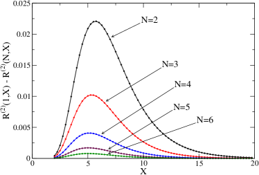
Figure 1: Large $N$ behaviour of the topological susceptibility for $g=2$: deviations of $R^{(2)}(N,X)$ from $R^{(2)}(1,X)$ are shown for $N$ up to $6$.

III The large $N$ limit

In this section we want to investigate the large $N$ behaviour of the topological susceptibility and, as previously anticipated, the most interesting case will be the $g=0$ case, since in Douglas:1993iia a third order phase transition was shown to be present (for $\theta=0$) in the large $N$ limit of continuum $U(N)$ gauge theories for $g=0$. This Douglas-Kazakov transition separates a “small area” region from a “large area” one, and it is located at $X=\pi^{2}$.

In trying to extend the Douglas-Kazakov approach to the $\theta\neq 0$ case, one could think of writing a large $N$ effective action starting from the partition function in Eq. (2) and using ${\hat{\theta}}=\theta/N$ as scaling variable (as was done e.g. in Bonati:2019ylr ; Rossi:2016uce following the original proposal of Witten:1980sp ). This approach seems however problematic: the contributions of representations corresponding to $\{l_{i}\}$ and $\{l_{i}+n\}$ (i.e. differing just for a $U(1)$ factor) differ in the large $N$ limit just by sub-leading terms, but in the thermodynamic limit the topological susceptibility coincides with that of the $U(1)$ model, and we can not expect the $U(1)$ degrees of freedom to be irrelevant. It thus seems more appropriate to construct an effective action for $\tilde{W}^{(g)}(N,X,k)$, and then use Eq. (23).

Introducing the continuous variable $y=i/N$ running from $-1/2$ to $1/2$, and the (decreasing) function $m(y)=m_{i}/N$, we may define the distribution $\rho(m)=-\mathrm{d}y/\mathrm{d}m$ and the large $N$ functional $S_{\mathrm{eff}}^{(g)}$ given by

$$S_{\mathrm{eff}}^{(g)}[m;X,k]\equiv-\lim_{N\to\infty}\frac{1}{N^{2}}\ln\tilde{W}^{(g)}(N,X,k)=$$ (27)

$$=(g-1)\left(\int\rho(m)\rho(m^{\prime})\ln|m-m^{\prime}|\mathrm{d}m\,\mathrm{d}m^{\prime}+\frac{3}{2}\right)+$$

$$+\frac{1}{2}X\left(\int\rho(m)m^{2}\mathrm{d}m-\bar{m}^{2}-\frac{1}{12}\right)-2\pi i\hat{k}\,\bar{m}\ ,$$

where we defined

$$\hat{k}\equiv\frac{k}{N}\ ,\quad\bar{m}\equiv\int m\,\rho(m)\mathrm{d}m$$ (28)

in order to simplify the notation. In Douglas:1993iia the integration domain had to be dynamically defined by the conditions $\int\rho(m)\mathrm{d}m=1$ and $0\leq\rho(m)\leq 1$, but now $\rho(m)$ is in general complex.

When $g>1$ the problem is singular, since for $\rho(m)\to 1$ the value of $S_{\mathrm{eff}}^{(g)}$ approaches $-\infty$. As a consequence, since $\rho(m)=1$ corresponds to $m(y)=-y$ (the additive constant being fixed by the constraint $m(1/2)=-1/2$) and thus to the trivial representation of $SU(N)$, for $g>1$ we recover the previously described trivial limit $\tilde{W}^{(g)}\to 1$ and the decoupling between $SU(N)$ and $U(1)$, a conclusion that is fully supported by the numerical results shown in Fig. 1.

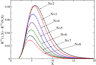
Figure 2: Large $N$ behaviour of the topological susceptibility for $g=1$: deviations of $R^{(1)}(N,X)$ from $R^{(1)}(1,X)$ are shown for $N$ up to $8$.

In the case $g=1$ it is known that the large $N$ expansion of the free energy starts at order $N^{0}$ for $\theta=0$ (see Gross:1992tu ; Gross:1993hu ; Gross:1993yt and Douglas:1993iia ), so the basic assumption used to obtain Eq. (27) is not true in this case and such an approach can not be pursued further. One could guess, by continuity in $g$, that also in this case the topological susceptibility in the large $N$ limit coincides with that of the $U(1)$ case. This is strongly supported by the numerical computations presented in Fig. 2, where the difference $R^{(1)}(N,X)-R^{(1)}(1,X)$ is shown (where $R^{(g)}$ is the normalized topological susceptibility defined in Eq. (11)). It is likely that this result could be obtained directly, starting from Eq. (2) and using the method developed in Gross:1992tu ; Gross:1993hu ; Gross:1993yt , in which case the $O(N^{-2})$ corrections of the topological susceptibiliy could maybe also be determined.

In the following we will concentrate on the analysis of the $g=0$ case, in which case stationary points of $S_{\mathrm{eff}}^{(0)}$ are solutions of the saddle point equation

$$-\,\mathrm{P}\!\!\int\frac{\rho(s)}{m-s}\mathrm{d}s+\frac{1}{2}X(m-\bar{m})-i\pi\hat{k}=0\ .$$ (29)

Since we are interested just to the first $\mathcal{O}(\hat{k}^{2})$ correction to the free energy, following the same approach used in Bonati:2019ylr we now introduce the Ansatz

$$\rho(m)=\rho_{0}(m)+i\hat{k}\,\rho_{1}(m)\ ,$$ (30)

where $\rho_{0}(m)$ is a real even function of $m$ and $\rho_{1}(m)$ is a real odd function of $m$. The conditions $\int\rho_{0}(m)\mathrm{d}m=1$ and $0\leq\rho_{0}(m)\leq 1$ now determine the integration domain of $\rho_{0}(m)$ and, since we are interested to the leading order in $\hat{k}$, we can assume $\rho_{1}(m)$ to have the same support of $\rho_{0}(m)$. The saddle-point equation Eq. (29) thus gives for $\rho_{0}$ and $\rho_{1}$ the equations

$$\mathrm{P}\!\!\int\frac{\rho_{0}(s)}{m-s}\mathrm{d}s=\frac{1}{2}X\,m\ ,$$ (31)

$$\mathrm{P}\!\!\int\frac{\rho_{1}(s)}{m-s}\mathrm{d}s=-\frac{1}{2}X\int s\,\rho_{1}(s)\mathrm{d}s-\pi\ .$$ (32)

For $X\leq\pi^{2}$ the solution of Eq. (31) is the Wigner semicircle law

$$\rho_{0}(m)=\frac{X}{2\pi}\sqrt{m_{0}^{2}-m^{2}}\ ,\quad m_{0}=\frac{2}{\sqrt{X}}\ ,$$ (33)

which fixes the integration domain to be $[-m_{0},m_{0}]$. For $X>\pi^{2}$ the semicircle law would predict $\rho_{0}(0)>1$ and the saddle point equation Eq. (31) has to be modified, in order to make it compatible with an Ansatz of the form

$$\rho_{0}(m)=\left\{\begin{array}[]{ll}1&\mathrm{for\ }|m|\leq b\\ \tilde{\rho}_{0}(m)&\mathrm{for\ }|m|>b\end{array}\right.\ ,$$ (34)

where $b$ has to be determined self-consistently, see Douglas:1993iia for a complete discussion.

When $X\leq\pi^{2}$ the domain of integration to be used in Eq. (32) is thus $[-m_{0},m_{0}]$ and this equation can be conveniently rewritten in the form

$$\mathrm{P}\!\!\int_{-m_{0}}^{m_{0}}\frac{\rho_{1}(s)}{m-s}\mathrm{d}s=C\ ,\quad C=-\frac{1}{2}X\int_{-m_{0}}^{m_{0}}s\,\rho_{1}(s)\mathrm{d}s-\pi\ .$$ (35)

If we introduce as usual Brezin:1977sv the resolvent $F(z)=\int\frac{\rho_{1}(s)}{z-s}\mathrm{d}s$ it is simple to show that the resolvent corresponding to the first equation is

$$F(z)=C\left(1-\frac{z}{\sqrt{z^{2}-m_{0}^{2}}}\right)$$ (36)

from which it follows that

$$\rho_{1}(m)=-\frac{C}{\pi}\frac{m}{\sqrt{m^{2}-m_{0}^{2}}}\ .$$ (37)

We can now substitute this expression in the second equation in Eq. (35) to fix $C$, however it is simple to show that (since $m_{0}^{2}X/4=1$) the resulting equation has no solution. We thus conclude that for $g=0$ and $X\leq\pi^{2}$ the saddle point equation Eq. (32) has no solution, and we take this fact as an indication that the topological susceptibility vanishes in the large $N$ limit (since a nontrivial solution for $\rho_{1}$ would give a susceptibility of order $N^{0}$).

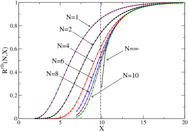
Figure 3: Large $N$ behaviour of the topological susceptibility for $g=0$. The vertical line at $X=\pi^{2}$ denotes the position of the Douglas-Kazakov transition. For $10\leq X\leq 11$ the $N\to\infty$ extrapolation of $R^{(0)}(N,X)$ is also shown, which is obtained from the results of Monte-Carlo simulations performed at $N\geq 30$, see the text for more details.

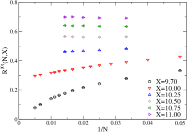
Figure 4: Large $N$ behaviour of the topological susceptibility for $g=0$ and several $X$ values.

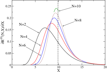
Figure 5: Large $N$ behaviour of $\partial R^{(0)}(N,X)/\partial X$. For the $N$ values shown in this figure the peak seems to approach the Douglas-Kazakov transition, indicated by the dashed vertical line.

For $X>\pi^{2}$ the saddle point equation for $\rho_{0}$ has to be modified in order for its solution to satisfy the requirement $\rho_{0}(m)\leq 1$ Douglas:1993iia , but it is not clear if the equation for $\rho_{1}$ has also to be modified (and eventually how). In absence of a clear theoretical understanding of this point, the following analysis will be based exclusively on numerical evidence.

In Fig. 3 we report the behaviour of the normalized topological susceptibility $R^{(0)}(N,X)$ (defined in Eq. (11)) for some values of $N$, up to $N=10$. It is clear that lines corresponding to increasing $N$ values are not converging to the $N=1$ curve. For $X$ smaller than $\pi^{2}$ the values of $R^{(0)}(N,X)$ seem to approach zero as $N$ grows, while for $X$ larger than $\pi^{2}$ they seem to converge to nonzero values in the same limit. Around $\pi^{2}$ a transition region is present, in which the behaviour of $R^{(0)}(N,X)$ rapidly changes.

These results have been obtained by explicitly performing the sums over $\{m_{i}\}$ up to a prescribed relative accuracy of $10^{-6}$ (the sum on $n$ can be rewritten in term of Jacobi $\theta$-functions), however, in order to reach larger values of $N$, we found computationally much more efficient to estimate average values using a Monte-Carlo sampling of the distribution in Eq. (7). Using this approach we obtained the data shown in Fig. 4, where the large $N$ behaviour of $R^{(0)}(N,X)$ is scrutinized for two values of $X$ close to $\pi^{2}\approx 9.8696$ ($X=9.7$ and $X=10$) using values of $N$ up to 200, and for larger $X$ values using $30\leq N\leq 70$. The large $N$ behaviour of the topological susceptibility is consistent with the one guessed from the results obtained using $N\leq 10$, however values of $N$ larger than $50$ are needed to clearly appreciate this behaviour for the two $X$ values closer to $\pi^{2}$. From these data we extracted the large $N$ limit of $R^{(0)}(N,X)$ shown in Fig. 3 for $10\leq X\leq 11$.

Data presented so far indicate that for $g=0$ manifolds the large $N$ topological susceptibility vanishes for $X<\pi^{2}$ while it is nonzero for larger values of $X$, approaching the $U(1)$ values as $X\gg 1$. From Figs. 3-4 we can see that the transition between the two regimes is quite abrupt, but we have no real hints on what happens at $X=\pi^{2}$. To further investigate the region $X\simeq\pi^{2}$ it is convenient to study $\partial R^{(0)}(N,X)/\partial X$ (see Eq. (12) for the explicit expression of this quantity), in order to understand if this observable develops a singularity at $X=\pi^{2}$ as $N$ gets larger.

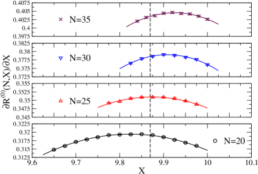
Figure 6: Large $N$ behaviour of $\partial R^{(0)}(N,X)/\partial X$. The dashed vertical line denotes the location of the Douglas-Kazakov transition and it is clear that the peak moves into the large area phase. Continuous lines are quadratic fit and they are drawn just to guide the eye.

In Fig. 5 the profile of $\partial R^{(0)}(N,X)/\partial X$ is shown for some $N$ values up to $N=10$, and a singularity at $X=\pi^{2}$ indeed seems to emerge. In order to reach larger $N$ values and better investigate this “might be” singular behaviour we again resorted to Monte-Carlo simulations, and the results obtained in this way are shown in Fig. 6. By looking just at data corresponding to $N\lesssim 25$ one could guess that the position of the peak of $\partial R^{(0)}(N,X)/\partial X$ approaches $\pi^{2}$, however data at larger $N$ show that the peak crosses the Douglas-Kazakov transition, going into the large-area regime. This is consistent with a continuous behaviour of $\partial R^{(0)}(N,X)/\partial X$ at the transition at $X=\pi^{2}$. Note however that this behaviour is formally continuous but nonetheless very abrupt, indeed for $X\lesssim 35$ the peak-value of $\partial R^{(0)}(N,X)/\partial X$ is still growing almost linearly in $N$ and its location is still very close to that of the Douglas-Kazakov transition.

IV Conclusions

In this paper we investigated the finite volume $\theta$-dependence of continuum two dimensional $U(N)$ gauge theories. We previously noted in Bonati:2019ylr that at finite volume the $U(1)$ degrees of freedom do not factorize in the partition function of 2d $U(N)$ gauge theories, even in the continuum limit. The continuum partition function was however written in a way that made the form of the interaction between the $U(1)$ and the $SU(N)$ degrees of freedom non completely clear.

In the present work we showed that the $\theta$-dependent continuum partition function can be rewritten in the more transparent form in Eq. (23). In this new form $\theta$ couples only to the $U(1)$ instanton number, but the effective action of the $SU(N)$ degrees of freedom generically depends on the topological charge of the background $U(1)$ field. In some specific limits, like in the thermodynamical limit ($X\to\infty$) or in the large genus limit ($g\to\infty$), this dependence disappears; only in these cases the $\theta$-dependence of the continuum 2d $U(N)$ theory reduces to that of the continuum $U(1)$ theory.

We then investigated the large $N$ behaviour of the topological susceptibility, mainly by means of numerical simulations. We found that, in the large $N$ limit and for fixed area of the manifold, the topological susceptibility converges to its $U(1)$ value only if the genus of the manifold is larger than zero.

In the case of a manifold with the topology of the sphere, the large $N$ topological susceptibility turned out to be an order parameter for the Douglas-Kazakov transition at $\theta=0$ Douglas:1993iia : the large $N$ limit of the topological susceptibility vanishes in the small-area phase $X<\pi^{2}$ and it is different from zero in the large-area phase. Moreover the derivative with respect to the area of the topological susceptibility is continuous across the transition.

This behaviour is the analogous, in the continuum finite area case, of the one previously found in Bonati:2019ylr , where the large $N$ behaviour of the topological susceptibility was shown to be different in the two phases of the Gross-Witten-Wadia transition. However for the case studied in Bonati:2019ylr an explicit analytic expression for the large $N$ topological susceptibility was found, while in the present case we had to rely mostly on numerics.

- (1) C. Bonati and P. Rossi, Phys. Rev. D 99, 054503 (2019) [arXiv:1901.09830 [hep-lat]].
- (2) B. E. Rusakov, Mod. Phys. Lett. A 5, 693 (1990).
- (3) E. Witten, Commun. Math. Phys. 141, 153 (1991).
- (4) J. Kiskis, R. Narayanan and D. Sigdel, Phys. Rev. D 89, 085031 (2014) [arXiv:1403.1770 [hep-th]].
- (5) D. J. Gross and E. Witten, Phys. Rev. D 21, 446 (1980).
- (6) S. R. Wadia, Phys. Lett. 93B, 403 (1980).
- (7) P. Rossi, Phys. Lett. 117B, 72 (1982).
- (8) M. R. Douglas and V. A. Kazakov, Phys. Lett. B 319, 219 (1993) [hep-th/9305047].
- (9) J. M. Drouffe and J. B. Zuber, Phys. Rept. 102, 1 (1983).
- (10) C. Cao, M. van Caspel and A. R. Zhitnitsky, Phys. Rev. D 87, 105012 (2013) [arXiv:1301.1706 [hep-th]].
- (11) P. Rossi, Phys. Rev. D 94, 4, 045013 (2016) [arXiv:1606.07252 [hep-th]].
- (12) E. Witten, Annals Phys. 128, 363 (1980).
- (13) D. J. Gross, Nucl. Phys. B 400, 161 (1993) [hep-th/9212149].
- (14) D. J. Gross and W. Taylor, Nucl. Phys. B 400, 181 (1993) [hep-th/9301068].
- (15) D. J. Gross and W. Taylor, Nucl. Phys. B 403, 395 (1993) [hep-th/9303046].
- (16) E. Brezin, C. Itzykson, G. Parisi and J. B. Zuber, Commun. Math. Phys. 59, 35 (1978).