Stochastic regularity of general quadratic observables of high frequency waves

Abstract

We consider the wave equation with uncertain initial data and medium, when the wavelength $\varepsilon$ of the solution is short compared to the distance traveled by the wave. We are interested in the statistics for quantities of interest (QoI), defined as functionals of the wave solution, given the probability distributions of the uncertain parameters in the wave equation. Fast methods to compute this statistics require considerable smoothness in the mapping from parameters to the QoI, which is typically not present in the high frequency case, as the oscillations on the $\varepsilon$ scale in the wave field is inherited by the QoIs. The main contribution of this work is to identify certain non-oscillatory quadratic QoIs and show $\varepsilon$-independent estimates for the derivatives of the QoI with respect to the parameters, when the wave solution is replaced by a Gaussian beam approximation.

1 Introduction

Many physical phenomena can be described by propagation of high-frequency waves with stochastic parameters. For instance, an earthquake where seismic waves with uncertain epicenter travel through the layers of the Earth with uncertain soil characteristics represents one such problem stemming from geophysics. Similar problems arise e.g. in optics, acoustics or oceanography. By high frequency we understand that the wavelength is very short compared to the distance traveled by the wave.

As a simplified model of the wave propagation, we use the scalar wave equation

$$u^{\varepsilon}_{tt}(t,\mathbf{x},{\mathbf{y}})=c(\mathbf{x},{\mathbf{y}})^{2}\,\Delta u^{\varepsilon}(t,\mathbf{x},{\mathbf{y}}),\qquad \text{in }[0,T]\times{\mathbb{R}}^{n}\times\Gamma,$$ (1a)

$$u^{\varepsilon}(0,\mathbf{x},{\mathbf{y}})=B_{0}(\mathbf{x},{\mathbf{y}})\,e^{i\,\varphi_{0}(\mathbf{x},{\mathbf{y}})/\varepsilon}, \text{in }{\mathbb{R}}^{n}\times\Gamma,$$ (1b)

$$u^{\varepsilon}_{t}(0,\mathbf{x},{\mathbf{y}})=\varepsilon^{-1}B_{1}(\mathbf{x},{\mathbf{y}})\,e^{i\,\varphi_{0}(\mathbf{x},{\mathbf{y}})/\varepsilon}, \text{in }{\mathbb{R}}^{n}\times\Gamma,$$ (1c)

with highly oscillatory initial data, represented by the small wavelength $\varepsilon\ll 1$, and a stochastic parameter ${\mathbf{y}}\in\Gamma\subset\mathbb{R}^{N}$ which models the uncertainty. For realistic problems, the dimension $N$ of the stochastic space can be fairly large. Two sources of uncertainty are considered: the local speed, $c=c(\mathbf{x},\mathbf{y})$, and the initial data, $B_{0}=B_{0}(\mathbf{x},\mathbf{y})$, $B_{1}=B_{1}(\mathbf{x},\mathbf{y})$, $\varphi_{0}=\varphi_{0}(\mathbf{x},\mathbf{y})$. The solution is therefore also a function of the random parameter, $u^{\varepsilon}=u^{\varepsilon}(t,\mathbf{x},\mathbf{y})$.

The focus of this work is on the regularity of certain nonlinear functionals of the solution $u^{\varepsilon}$ with respect to the random parameters ${\mathbf{y}}$. Our motivation for the study comes from the field of uncertainty quantification (UQ), where the functionals represent quantities of interest (QoI). We will denote them generically by ${\mathcal{Q}}({\bf y})$. The aim in (forward) UQ is to compute the statistics of ${\mathcal{Q}}$, typically the mean and the variance, given the probability distribution of ${\bf y}$. This is often done by random sample based methods like Monte–Carlo [9], which, however, has a rather slow convergence rate; the error decays as $O(N^{-1/2})$ for $N$ samples. Grid based methods like Stochastic Galerkin (SG) [10, 34, 2, 32] and Stochastic Collocation (SC) [33, 3, 27] can achieve much faster convergence rates, even spectral rates where the error decays faster than $N^{-p}$ for all $p>0$. They rely on smoothness of ${\mathcal{Q}}({\bf y})$ with respect to ${\bf y}$. This smoothness is referred to as the stochastic regularity of the problem. When ${\bf y}$ is a high-dimensional vector, SG and SC must be performed on sparse grids [5, 11] to break the curse of dimension. This typically requires even stronger stochastic regularity.

To show the fast convergence of SG and SC, analysis of the stochastic regularity has been carried out for many different PDE problems. Examples include elliptic problems [1, 7, 26], the wave equation [25], Maxwell equations [17] and various kinetic equations [14, 18, 21, 16, 30].

In the high frequency case, which is the subject of this article, the main question is how the ${\mathbf{y}}$-derivatives of ${\mathcal{Q}}$ depend on the wave length $\varepsilon$. The solution $u^{\varepsilon}$ oscillates with period $\varepsilon$ and these oscillations are often inherited by ${\mathcal{Q}}$. If this is the case, SG and SC will not work well, as the derivatives of ${\mathcal{Q}}$ grow rapidly with $\varepsilon$. Special choices of ${\mathcal{Q}}$ can, however, have better properties, as we discuss below. A further complication is that the direct numerical solution of (1) becomes infeasible as $\varepsilon\to 0$, as the computational cost to approximate $u^{\varepsilon}$ is of order $O(\varepsilon^{-n-1})$. Asymptotic methods based on e.g. geometrical optics [8, 29] or Gaussian beams (GB) [6, 28] must therefore be used.

In [24] we identified a non-oscillatory quadratic QoI,

$$\widetilde{\mathcal{Q}}(t,\mathbf{y}):=\int_{\mathbb{R}^{n}}|u^{\varepsilon}(t,\mathbf{x},\mathbf{y})|^{2}\psi(t,\mathbf{x})\,d\mathbf{x},\qquad\psi\in C_{c}^{\infty}(\mathbb{R}\times\mathbb{R}^{n}),$$ (2)

and introduced a GB solver for $u^{\varepsilon}$ coupled with SC on sparse grids to approximate it. A big advantage of the GB method is that it approximates the solution to the PDE (1) via solutions to a set of $\varepsilon$-independent ODEs instead. In [23] we also showed rigorously that all derivatives of $\widetilde{\mathcal{Q}}$ are bounded independently of $\varepsilon$ when the wave solution $u^{\varepsilon}$ is approximated by Gaussian beams,

$$\sup_{\mathbf{y}\in\Gamma}\left|\frac{\widetilde{\mathcal{Q}}(t,\mathbf{y})}{\partial\mathbf{y}^{\boldsymbol{\sigma}}}\right|\leq C_{\boldsymbol{\sigma}},\qquad\forall\boldsymbol{\sigma}\in\mathbb{N}_{0}^{N},$$

where $C_{\boldsymbol{\sigma}}$ are independent of $\varepsilon$. A related study is found in [15].

In this article we generalize the result in [23] and consider QoIs which include higher order derivatives of the solution and also averaging in time. More precisely, we study

$$\mathcal{Q}^{p,\boldsymbol{\alpha}}(\mathbf{y})=\varepsilon^{2(p+|\boldsymbol{\alpha}|)}\int_{\mathbb{R}}\int_{\mathbb{R}^{n}}g(t,\mathbf{x},\mathbf{y})|\partial_{t}^{p}\partial_{\mathbf{x}}^{\boldsymbol{\alpha}}u^{\varepsilon}(t,\mathbf{x},\mathbf{y})|^{2}\psi(t,\mathbf{x})\,d\mathbf{x}\,dt,$$ (3)

with $g\in C^{\infty}(\mathbb{R}\times\mathbb{R}^{n}\times\Gamma)$, $p$ a non-negative integer and ${\boldsymbol{\alpha}}$ a multi-index. Many physically relevant QoIs can be written on this form. The simplest case in (3),

$$\mathcal{Q}(\mathbf{y}):=\mathcal{Q}^{0,\mathbf{0}}(\mathbf{y})=\int_{\mathbb{R}}\int_{\mathbb{R}^{n}}|u^{\varepsilon}(t,\mathbf{x},\mathbf{y})|^{2}\psi(t,\mathbf{x})\,d\mathbf{x}\,dt,$$ (4)

represents the weighted average intensity of the wave. If the solution $u^{\varepsilon}$ to (1) describes the pressure, then $\mathcal{Q}$ represents the acoustic potential energy. Another significant example is the weighted total energy of the wave,

$$E(\mathbf{y})=\varepsilon^{2}\int_{\mathbb{R}}\int_{\mathbb{R}^{n}}(|u_{t}^{\varepsilon}(t,\mathbf{x},\mathbf{y})|^{2}+c^{2}(\mathbf{x},\mathbf{y})|\nabla u^{\varepsilon}(t,\mathbf{x},\mathbf{y})|^{2})\psi(t,\mathbf{x})\,d\mathbf{x}\,dt,$$

which can be decomposed into terms of type (3). An additional example is the weighted and averaged version of the Arias intensity,

$$I(\mathbf{y})=\varepsilon^{4}\int_{\mathbb{R}}\int_{\mathbb{R}^{n}}|u_{tt}^{\varepsilon}(t,\mathbf{x},\mathbf{y})|^{2}\psi(t,\mathbf{x})\,d\mathbf{x}\,dt,$$

which represents the total energy per unit mass and is used to measure the strength of ground motion during an earthquake, see [12].

In this work we show that also the QoI (3) is non-oscillatory when $u^{\varepsilon}$ is replaced by the GB approximation $\tilde{u}$. Indeed, under the assumptions given in Section 2 we then prove that for all compact $\Gamma_{c}\subset\Gamma$ and all $\boldsymbol{\sigma}\in\mathbb{N}_{0}^{N}$,

$$\sup_{\mathbf{y}\in\Gamma_{c}}\left|\frac{\partial^{\boldsymbol{\sigma}}\mathcal{Q}^{p,\boldsymbol{\alpha}}(\mathbf{y})}{\partial\mathbf{y}^{\boldsymbol{\sigma}}}\right|\leq C_{\boldsymbol{\sigma}},$$ (5)

for some constants $C_{\boldsymbol{\sigma}}$, uniformly in $\varepsilon$.

The full GB approximation $\tilde{u}$ features two modes, $\tilde{u}=\tilde{u}^{+}+\tilde{u}^{-}$, satisfying two different sets of ODEs. In certain cases, it is possible to approximate $u^{\varepsilon}$ by one of the modes only, i.e. either $\tilde{u}=\tilde{u}^{+}$ or $\tilde{u}=\tilde{u}^{-}$. We can then examine a QoI that, in contrast to (3), is only integrated in space,

$$\widetilde{\mathcal{Q}}^{p,\boldsymbol{\alpha}}(t,\mathbf{y})=\varepsilon^{2(p+|\boldsymbol{\alpha}|)}\int_{\mathbb{R}^{n}}g(t,\mathbf{x},\mathbf{y})|\partial_{t}^{p}\partial_{\mathbf{x}}^{\boldsymbol{\alpha}}u^{\varepsilon}(t,\mathbf{x},\mathbf{y})|^{2}\psi(t,\mathbf{x})\,d\mathbf{x},$$ (6)

and show a stronger regularity result,

$$\sup_{\begin{subarray}{c}\mathbf{y}\in\Gamma_{c}\\ t\in[0,T]\end{subarray}}\left|\frac{\partial^{\boldsymbol{\sigma}}\widetilde{\mathcal{Q}}^{p,\boldsymbol{\alpha}}(t,\mathbf{y})}{\partial\mathbf{y}^{\boldsymbol{\sigma}}}\right|\leq C_{\boldsymbol{\sigma}},\qquad\forall\boldsymbol{\sigma}\in\mathbb{N}_{0}^{N},$$ (7)

uniformly in $\varepsilon$, when $u^{\varepsilon}$ is replaced by $\tilde{u}^{\pm}$. In fact, this one-mode case, with $p={\boldsymbol{\alpha}}=0$, was the one considered in [23].

The layout of this article is as follows: we briefly introduce our assumptions in Section 2 and then present the Gaussian beam method in Section 3. The one-mode QoI (6) with $u^{\varepsilon}$ approximated by $\tilde{u}=\tilde{u}^{\pm}$ is regarded in Section 4. The stochastic regularity (7) is shown in Theorem 4.2. This serves as a stepping stone for the proof of regularity of the general two-mode QoI (3) with $u^{\varepsilon}$ approximated by $\tilde{u}=\tilde{u}^{+}+\tilde{u}^{-}$, which is the subject of Section 5 where the final stochastic regularity (5) is shown in Theorem 5.2.

2 Assumptions and preliminaries

Let us consider the Cauchy problem (1). By $t\in[0,T]\subset\mathbb{R}$ we denote the time, $\mathbf{x}=(x_{1},\ldots,x_{n})\in\mathbb{R}^{n}$ is the spatial variable and the uncertainty in the model is described by the random variable $\mathbf{y}=(y_{1},\ldots y_{N})\in\Gamma$ where $\Gamma\subset\mathbb{R}^{N}$ is an open set. By ${\mathcal{B}}_{\mu}$ we will denote the $n$-dimensional closed ball around 0 of radius $\mu$, i.e. the set ${\mathcal{B}}_{\mu}:=\{\mathbf{x}\in\mathbb{R}^{n}:|\mathbf{x}|\leq\mu\}$, with the convention that ${\mathcal{B}}_{\infty}=\mathbb{R}^{n}$.

We make the following precise assumptions.

1. Strictly positive, smooth and bounded speed of propagation,

   $$c\in C^{\infty}(\mathbb{R}^{n}\times\Gamma),\qquad 0<c_{\rm min}\leq c(\mathbb{x},{\bf y})\leq c_{\rm max}<\infty,\qquad\forall\,{\bf x}\in{\mathbb{R}}^{n},\quad\forall\,{\bf y}\in\Gamma.$$

   and for each multi-index pair $\boldsymbol{\alpha}$, $\boldsymbol{\beta}$ there is a constant $C_{\boldsymbol{\alpha},\boldsymbol{\beta}}$ such that

   $$\left|\partial_{\bf x}^{\boldsymbol{\alpha}}\partial_{\bf y}^{\boldsymbol{\beta}}c({\bf x},{\bf y})\right|\leq C_{\boldsymbol{\alpha},\boldsymbol{\beta}},\qquad\forall\,{\bf x}\in{\mathbb{R}}^{n},\quad\forall\,{\bf y}\in\Gamma.$$

2. Smooth and (uniformly) compactly supported initial amplitudes,

   $$B_{{\ell}}\in C^{\infty}(\mathbb{R}^{n}\times\Gamma),\qquad{\rm supp}\,B_{{\ell}}(\,\cdot\,,{\bf y})\subset K_{0},\qquad\ell=0,1,\quad\forall\,\mathbf{y}\in\Gamma,$$

   where $K_{0}\subset\mathbb{R}^{n}$ is a compact set.

3. Smooth initial phase with non-zero gradient,

   $$\varphi_{0}\in C^{\infty}(\mathbb{R}^{n}\times\Gamma),\qquad|\nabla\varphi_{0}({\bf x},{\bf y})|>0,\qquad\forall\,{\bf x}\in{\mathbb{R}}^{n},\quad\forall\,{\bf y}\in\Gamma.$$

4. High frequency,

   $$0<\varepsilon\leq 1.$$

5. Smooth and compactly supported QoI test function,

   $$\psi\in C^{\infty}_{c}(\mathbb{R}\times\mathbb{R}^{n}),\qquad\text{supp}\,\psi\subset[0,T]\times K_{1},$$

   where $K_{1}\subset\mathbb{R}^{n}$ is a compact set.

Throughout the paper we will frequently use the shorthand $f\in C^{\infty}$ with the understanding that $f$ is continuously differentiable infinitely many times in each of its variables, over its entire domain of definition, typically $\mathbb{R}\times\mathbb{R}^{n}\times\Gamma\times\mathbb{R}^{n}$ or $\mathbb{R}\times\mathbb{R}^{n}\times\Gamma\times\mathbb{R}^{n}\times\mathbb{R}^{n}$.

3 Gaussian beam approximation

Solving (1) directly requires a substantial number of numerical operations when the wavelength $\varepsilon$ is small. In particular, to maintain a given accuracy for a fixed $\mathbf{y}$, we need at least $O(\varepsilon^{-n})$ discretization points in $\mathbf{x}$ and $O(\varepsilon^{-1})$ time steps resulting into the computational cost $O(\varepsilon^{-n-1})$. To avoid the high cost we employ asymptotic methods arising from geometrical optics. In particular, the Gaussian beam (GB) method provides a powerful tool, see [6, 19, 28, 29, 31].

Individual Gaussian beams are asymptotic solutions to the wave equation (1) that concentrate around a central ray in space-time. Rays are bicharacteristics of the wave equation (1). They are denoted by $(\mathbf{q}^{\pm},\mathbf{p}^{\pm})$ where $\mathbf{q}^{\pm}(t,\mathbf{y},\mathbf{z})$ represents the position and $\mathbf{p}^{\pm}(t,\mathbf{y},\mathbf{z})$ the direction, respectively, and $\mathbf{z}\in K_{0}$ is the starting point so that $\mathbf{q}^{\pm}(0,\mathbf{y},\mathbf{z})=\mathbf{z}$ for all $\mathbf{y}\in\Gamma$. From each $\mathbf{z}$, the ray propagates in two opposite directions, here distinguished by the superscript $\pm$. These corresponds to the two modes of the wave equation and leads to two different GB solutions, one for each mode. We denote the two $k$-th order Gaussian beams starting at $\mathbf{z}\in K_{0}$ by $v_{k}^{\pm}(t,\mathbf{x},\mathbf{y},\mathbf{z})$ and define it as

$$v_{k}^{\pm}(t,\mathbf{x},\mathbf{y},\mathbf{z})=A_{k}^{\pm}(t,\mathbf{x}-\mathbf{q}^{\pm}(t,\mathbf{y},\mathbf{z}),\mathbf{y},\mathbf{z})e^{i\Phi_{k}^{\pm}(t,\mathbf{x}-\mathbf{q}^{\pm}(t,\mathbf{y},\mathbf{z}),\mathbf{y},\mathbf{z})/\varepsilon},$$ (8)

where

$$\Phi_{k}^{\pm}(t,\mathbf{x},\mathbf{y},\mathbf{z})=\phi_{0}^{\pm}(t,\mathbf{y},\mathbf{z})+\mathbf{x}^{T}\mathbf{p}^{\pm}(t,\mathbf{y},\mathbf{z})+\frac{1}{2}\,\mathbf{x}^{T}M^{\pm}(t,\mathbf{y},\mathbf{z})\mathbf{x}+\sum_{|\boldsymbol{\beta}|=3}^{k+1}\frac{1}{\boldsymbol{\beta}!}\phi_{\boldsymbol{\beta}}^{\pm}(t,\mathbf{y},\mathbf{z})\mathbf{x}^{\boldsymbol{\beta}},$$ (9)

is the $k$-th order phase function and

$$A_{k}^{\pm}(t,\mathbf{x},\mathbf{y},\mathbf{z})=\sum_{j=0}^{\lceil\frac{k}{2}\rceil-1}\varepsilon^{j}\sum_{|\boldsymbol{\beta}|=0}^{k-2j-1}\frac{1}{\boldsymbol{\beta}!}a_{j,\boldsymbol{\beta}}^{\pm}(t,\mathbf{y},\mathbf{z})\mathbf{x}^{\boldsymbol{\beta}},$$ (10)

is the $k$-th order amplitude function. The higher the order $k$, the more accurately $v_{k}^{\pm}$ approximates the solution to (1) in terms of $\varepsilon$. The variables $\phi_{0}^{\pm},\mathbf{q}^{\pm},\mathbf{p}^{\pm},M^{\pm},\phi_{\boldsymbol{\beta}}^{\pm},a_{j,\boldsymbol{\beta}}^{\pm}$ are given by a set of ODEs, the simplest ones being

$$\dot{\phi}_{0}^{\pm} =0,$$ (11a)

$$\dot{\mathbf{q}}^{\pm} =\pm c(\mathbf{q}^{\pm})\frac{\mathbf{p}^{\pm}}{|\mathbf{p}^{\pm}|},$$ (11b)

$$\dot{\mathbf{p}}^{\pm} =\mp\nabla c(\mathbf{q}^{\pm})|\mathbf{p}^{\pm}|,$$ (11c)

$$\dot{M}^{\pm} =\mp(D^{\pm}+(B^{\pm})^{T}M^{\pm}+M^{\pm}B^{\pm}+M^{\pm}C^{\pm}M^{\pm}),$$ (11d)

$$\dot{a}_{0,\mathbf{0}}^{\pm} =\pm\frac{1}{2|\mathbf{p}^{\pm}|}\left(-c(\mathbf{q}^{\pm})\text{Tr}(M^{\pm})+\nabla c(\mathbf{q}^{\pm})^{T}\mathbf{p}^{\pm}+\frac{c(\mathbf{q}^{\pm})(\mathbf{p}^{\pm})^{T}M^{\pm}\mathbf{p}^{\pm}}{|\mathbf{p}^{\pm}|^{2}}\right)a_{0,\mathbf{0}}^{\pm},$$ (11e)

where

$$B^{\pm}=\frac{\mathbf{p}^{\pm}\nabla c(\mathbf{q}^{\pm})^{T}}{|\mathbf{p}^{\pm}|},\qquad C^{\pm}=\frac{c(\mathbf{q}^{\pm})}{|\mathbf{p}^{\pm}|}-\frac{c(\mathbf{q}^{\pm})}{|\mathbf{p}^{\pm}|^{3}}\mathbf{p}^{\pm}(\mathbf{p}^{\pm})^{T},\qquad D^{\pm}=|\mathbf{p}^{\pm}|\nabla^{2}c(\mathbf{q}^{\pm}).$$

For the ODEs determining $\phi_{\boldsymbol{\beta}}^{\pm}$ and $a_{j,\boldsymbol{\beta}}^{\pm}$ other than the leading term we refer the reader to [28, 31].

As mentioned above, the sign corresponds to GBs moving in opposite directions which means that they constitute two different modes that are governed by two different sets of ODEs. Single beams from the same mode with their starting points in $K_{0}$ are summed together to form the $k$-th order one-mode solution $u_{k}^{\pm}(t,\mathbf{x},\mathbf{y})$,

$$u^{\pm}_{k}(t,\mathbf{x},\mathbf{y})=\left(\frac{1}{2\pi\varepsilon}\right)^{n/2}\int_{K_{0}}v_{k}^{\pm}(t,\mathbf{x},\mathbf{y},\mathbf{z})\varrho_{\eta}(\mathbf{x}-\mathbf{q}^{\pm}(t,\mathbf{y},\mathbf{z}))d\mathbf{z}.$$ (12)

where the integration in $\mathbf{z}$ is over the support of the initial data $K_{0}\subset\mathbb{R}^{n}$, which is independent of ${\mathbf{y}}$ by (A2). Since the wave equation is linear, the superposition of beams is still an asymptotic solution. The function $\varrho_{\eta}\in C^{\infty}(\mathbb{R}^{n})$ is a real-valued cutoff function with radius $0<\eta\leq\infty$,

$$\varrho_{\eta}(\mathbf{x})=\left\{\begin{array}[]{lll}1,&\text{if }|\mathbf{x}|\leq\eta,&\text{for }0<\eta<\infty,\\ 0,&\text{if }|\mathbf{x}|\geq 2\eta,&\text{for }0<\eta<\infty,\\ 1,&&\text{for }\eta=\infty.\end{array}\right.$$ (13)

For first order GBs, $k=1$, one can choose $\eta=\infty$, i.e. no $\varrho_{\eta}$, see below.

Each GB $v_{k}^{\pm}$ requires initial values for all its coefficients. An appropriate choice makes $u_{k}^{\pm}(0,\mathbf{x},\mathbf{y})$ converge asymptotically as $\varepsilon\to 0$ to the initial conditions in (1). As shown in [19], the initial data are to be chosen as follows:

$$\mathbf{q}^{\pm}(0,\mathbf{y},\mathbf{z}) =\mathbf{z},$$ (14a)

$$\mathbf{p}^{\pm}(0,\mathbf{y},\mathbf{z}) =\nabla\varphi_{0}(\mathbf{z},\mathbf{y}),$$ (14b)

$$\phi^{\pm}_{0}(0,\mathbf{y},\mathbf{z}) =\varphi_{0}(\mathbf{z},\mathbf{y}),$$ (14c)

$$M^{\pm}(0,\mathbf{y},\mathbf{z}) =\nabla^{2}\varphi_{0}(\mathbf{z},\mathbf{y})+i\ I_{n\times n},$$ (14d)

$$\phi^{\pm}_{\boldsymbol{\beta}}(0,\mathbf{y},\mathbf{z}) =\partial_{\mathbf{x}}^{\boldsymbol{\beta}}\varphi_{0}(\mathbf{z},\mathbf{y}),\qquad|\boldsymbol{\beta}|=3,\ldots,k+1,$$ (14e)

$$a_{0,\mathbf{0}}^{\pm}(0,\mathbf{y},\mathbf{z}) =\frac{1}{2}\left(B_{0}(\mathbf{z},\mathbf{y})\pm\frac{B_{1}(\mathbf{z},\mathbf{y})}{ic(\mathbf{z},\mathbf{y})|\nabla\varphi_{0}(\mathbf{z},\mathbf{y})|}\right),$$ (14f)

where $I_{n\times n}$ denotes the identity matrix of size $n$. The initial data for the higher order amplitude coefficients are given in [19]. The following proposition shows that all these variables are smooth and $a_{j,\boldsymbol{\beta}}^{\pm}$ remain supported in $K_{0}$ for all times $t$ and random variables $\mathbf{y}\in\Gamma$.

Proposition 3.1.

Under assumptions (A1)–(A3), the coefficients $\phi_{0}^{\pm},\mathbf{q}^{\pm},\mathbf{p}^{\pm},M^{\pm},\phi_{\boldsymbol{\beta}}^{\pm},a_{j,\boldsymbol{\beta}}^{\pm}$ all belong to $C^{\infty}(\mathbb{R}\times\Gamma\times\mathbb{R}^{n})$ and

$$\text{\rm supp}(a_{j,\boldsymbol{\beta}}^{\pm}(t,\mathbf{y},\cdot))\subset K_{0},\qquad\forall\ t\in\mathbb{R},\,\mathbf{y}\in\Gamma.$$

Consequently, $\Phi_{k}^{\pm}\in C^{\infty}$.

Proof.

Existence and regularity of the solutions follow from standard ODE theory and a result in [28, Section 2.1] which ensures that the non-linear Riccati equations for $M^{\pm}(t,{\mathbf{y}};{\mathbf{z}})$ have solutions for all times and parameter values, with the given initial data. That $\text{supp}(a_{j,\boldsymbol{\beta}}^{\pm}(t,\mathbf{y},\cdot))$ stays in $K_{0}$ for all times is a consequence of the form of the ODEs for the amplitude coefficients, given in [28]. ∎

Finally, the $k$-th order GB superposition solution is defined as a sum of the two modes in (12),

$$u_{k}(t,\mathbf{x},\mathbf{y})=u^{+}_{k}(t,\mathbf{x},\mathbf{y})+u^{-}_{k}(t,\mathbf{x},\mathbf{y}).$$ (15)

Approximating $u^{\varepsilon}$ with $u_{k}$ we can define the GB quantity of interest corresponding to (3) as

$$\mathcal{Q}_{\text{GB}}^{p,\boldsymbol{\alpha}}(\mathbf{y})=\varepsilon^{2(p+|\boldsymbol{\alpha}|)}\int_{\mathbb{R}}\int_{\mathbb{R}^{n}}g(t,\mathbf{x},\mathbf{y})|\partial_{t}^{p}\partial_{\mathbf{x}}^{\boldsymbol{\alpha}}u_{k}(t,\mathbf{x},\mathbf{y})|^{2}\psi(t,\mathbf{x})d\mathbf{x}\,dt,$$ (16)

where $\psi$ is as in (A5) and $g\in C^{\infty}(\mathbb{R}\times\mathbb{R}^{n}\times\Gamma)$.

We note that for numerical computations with SG or SC combined with GB it is indeed the stochastic regularity of ${\mathcal{Q}}_{\text{GB}}^{p,\boldsymbol{\alpha}}$ rather than of the exact ${\mathcal{Q}}^{p,\boldsymbol{\alpha}}$ that is relevant. Moreover, since $u_{k}$ approximates the exact solution $u^{\varepsilon}$ well, ${\mathcal{Q}}_{\text{GB}}^{p,\boldsymbol{\alpha}}$ will also be a good approximation of ${\mathcal{Q}}^{p,\boldsymbol{\alpha}}$. For instance, when $p=0$ and $\alpha\neq 0$ one can use the Sobolev estimate $||u_{k}-u^{\varepsilon}||_{H^{s}}\leq C\varepsilon^{k/2-s}$, for $s\geq 1$, shown in [20], to derive the error bound $|{\mathcal{Q}}_{\text{GB}}^{0,\boldsymbol{\alpha}}-{\mathcal{Q}}^{0,\boldsymbol{\alpha}}|\leq C\varepsilon^{k/2}$ in the same way as in [23], where the case $\alpha=0$ was discussed. Also, in some cases, like in one dimension with constant speed $c(x,y)=c(y)$, the GB solution is exact if the initial data is exact. Then $\mathcal{Q}_{\text{GB}}^{p,\alpha}=\mathcal{Q}^{p,\alpha}$.

4 One-mode quantity of interest

Before considering the QoI (16) it is advantageous to first focus on its one-mode counterpart with $u_{k}$ consisting of either $u_{k}=u_{k}^{+}$ or $u_{k}=u_{k}^{-}$ only, as given in (6). In the present article, this is partly due to the fact that the one-mode QoI will be a stepping stone for our analysis of the full two-mode QoI. However, its examination is also important in its own right. As the two wave modes propagate in opposite directions they separate and parts of the domain will mainly be covered by waves belonging to only one of the modes. As a simple example, in one dimension with constant speed, the d’Alembert solution to the wave equation is a superposition of a left and a right going wave. In the general case, the effect is more pronounced in the high-frequency regime, when the wave length is significantly smaller than the curvature of the wave front [8, 29]. Discarding one of the modes then amounts to discarding reflected waves and waves that initially propagate away from the domain of interest. The solution will nevertheless contain waves going in different directions. For example, if $B_{1}$ in (1) is chosen such that $u^{\varepsilon}$ essentially propagates in one direction, then merely one mode, either $u_{k}^{+}$ or $u_{k}^{-}$, is sufficient to approximate $u^{\varepsilon}$. The approximation is similar to, but not the same as, using the paraxial wave equation instead of the full wave equation, which is a common strategy in areas like seismology, plasma physics, underwater acoustics and optics [4].

Let us thus define the GB-approximated version of the QoI in (6),

$$\widetilde{\mathcal{Q}}^{p,\boldsymbol{\alpha}}_{\text{GB}}(t,\mathbf{y})=\varepsilon^{2(p+|\boldsymbol{\alpha}|)}\int_{\mathbb{R}^{n}}g(t,\mathbf{x},\mathbf{y})|\partial_{t}^{p}\partial_{\mathbf{x}}^{\boldsymbol{\alpha}}u_{k}(t,\mathbf{x},\mathbf{y})|^{2}\psi(t,\mathbf{x})d\mathbf{x},$$ (17)

with $\psi\in C_{c}^{\infty}(\mathbb{R}\times\mathbb{R}^{n})$ and $g\in C^{\infty}(\mathbb{R}\times\mathbb{R}^{n}\times\Gamma)$. Here $u_{k}=u_{k}^{+}$ or $u_{k}=u_{k}^{-}$ in (15). It is not important which one we choose and henceforth omit superscripts of all variables.

To introduce the terminology used in this section, we will need the following proposition.

Proposition 4.1.

Assume (A1)–(A3) hold. Then for all $T>0$, beam order $k$ and compact $\Gamma_{c}\subset\Gamma$, there is a GB cutoff width $\eta>0$ and constant $\delta>0$ such that for all $\mathbf{x}\in{\mathcal{B}}_{2\eta}$,

$$\operatorname{Im}\Phi_{k}(t,\mathbf{x},\mathbf{y},\mathbf{z})\geq\delta|\mathbf{x}|^{2},\quad\forall t\in[0,T],\,\mathbf{y}\in\Gamma_{c},\,\mathbf{z}\in K_{0}.$$ (18)

For the first order GB, $k=1$, we can take $\eta=\infty$ and (18) is valid for all $\mathbf{x}\in\mathbb{R}^{n}$.

Proof.

Property (P4) in Proposition 1 in [23]. The proof is in [22]. ∎

Note that $\eta$ is the width of the cutoff function $\varrho_{\eta}$ in (13) used in the GB superposition (12).

Definition 1.

The cutoff width $\eta$ used for the GB approximation is called admissible for a given $T$, $k$ and $\Gamma_{c}$ if it is small enough in the sense of Proposition 4.1.

We will prove the following main theorem.

Theorem 4.2.

Assume (A1)–(A5) hold and consider a one-mode GB solution. Moreover, let $\eta$ be admissible for $T>0$, $k$ and a compact $\Gamma_{c}\subset\Gamma$. Then for all $p\in\mathbb{N}$ and $\boldsymbol{\alpha}\in\mathbb{N}_{0}^{N}$, there exist $C_{\boldsymbol{\sigma}}$ such that

$$\sup_{\begin{subarray}{c}\mathbf{y}\in\Gamma_{c}\\ t\in[0,T]\end{subarray}}\left|\frac{\partial^{\boldsymbol{\sigma}}\widetilde{\mathcal{Q}}^{p,\boldsymbol{\alpha}}_{\text{GB}}(t,\mathbf{y})}{\partial\mathbf{y}^{\boldsymbol{\sigma}}}\right|\leq C_{\boldsymbol{\sigma}},\quad\forall\boldsymbol{\sigma}\in\mathbb{N}_{0}^{N},$$

where $C_{\boldsymbol{\sigma}}$ is independent of $\varepsilon$ but depends on $T,k$ and $\Gamma_{c}$.

The proof of Theorem 4.2 is presented in Section 4.2.

Let us also recall the known results regarding the simplest version of the QoI (17),

$$\widetilde{\mathcal{Q}}_{\text{GB}}:=\widetilde{\mathcal{Q}}_{\text{GB}}^{0,\mathbf{0}}=\int_{\mathbb{R}^{n}}|u_{k}(t,\mathbf{x},\mathbf{y})|^{2}\psi(t,\mathbf{x})d\mathbf{x},$$ (19)

which were obtained in [23].

Theorem 4.3 ([23, Theorem 1]).

Assume (A1)–(A5) hold and consider a one-mode GB solution. Moreover, let $\eta$ be admissible for $T>0$, $k$ and a compact $\Gamma_{c}\subset\Gamma$. Then there exist $C_{\boldsymbol{\sigma}}$ such that

$$\sup_{\begin{subarray}{c}\mathbf{y}\in\Gamma_{c}\\ t\in[0,T]\end{subarray}}\left|\frac{\partial^{\boldsymbol{\sigma}}\widetilde{\mathcal{Q}}_{\text{GB}}(t,\mathbf{y})}{\partial\mathbf{y}^{\boldsymbol{\sigma}}}\right|\leq C_{\boldsymbol{\sigma}},\quad\forall\boldsymbol{\sigma}\in\mathbb{N}_{0}^{N},$$

where $C_{\boldsymbol{\sigma}}$ is independent of $\varepsilon$ but depends on $T$, $k$ and $\Gamma_{c}$.

Remark.

This is a minor generalization of Theorem 1 in [23]. In particular we here allow $\psi$ to also depend on $t$ and have an estimate that is uniform in $t$. Moreover, instead of assuming $\Gamma$ to be the closure of a bounded open set, as in [23], we consider compact subsets $\Gamma_{c}$ of an open set $\Gamma$. These modifications do not affect the proof in a significant way.

Remark.

One can note that the stochastic regularity in $\mathbf{y}$ shown in Theorem 4.2 also implies stochastic regularity in $t$ for the same QoI. Indeed, upon defining

$$v^{\varepsilon}(t,\mathbf{x},\mathbf{y},y_{0}):=u^{\varepsilon}(ty_{0},\mathbf{x},\mathbf{y}),$$

$v^{\varepsilon}$ will satisfy the same wave equation as $u^{\varepsilon}$, with $c(\mathbf{x},\mathbf{y})$ replaced by $y_{0}c(\mathbf{x},\mathbf{y})$ and $B_{1}(\mathbf{x},\mathbf{y})$ replaced by $y_{0}B_{1}(\mathbf{x},\mathbf{y})$. One can verify that with these alterations, the Gaussian beam approximations of $u^{\varepsilon}$ and $v^{\varepsilon}$ also satisfy the same equations. Moreover, for a fixed $t$, time derivatives of the QoI based on $u^{\varepsilon}$ corresponds to partial derivatives in $y_{0}$ for the QoI based on $v^{\varepsilon}$, which is covered by the theory above. However, making this observation precise, we leave for future work.

4.1 Preliminaries

In this section we introduce functions spaces and derive some preliminary results for the main proof of Theorem 4.2. However, we start with a note on the case $\eta=\infty$, which is sometimes an admissible cutoff width in the sense of Proposition 4.1. In particular, it is always admissible when $k=1$. It amounts to removing the cutoff functions $\varrho_{\eta}$ in (12) altogether. This is convenient in computations, but there are some technical issues with having $\eta=\infty$ in the proofs below. We note, however, that, in any finite time interval $[0,T]$ and compact $\Gamma_{c}\subset\Gamma$, the Gaussian beam superposition (15) with no cutoff is identical to the one with a large enough cutoff, because of the compact support of the test function $\psi(t,\mathbf{x})$. Indeed, suppose $\text{supp }\psi(t,\cdot)\subset{\mathcal{B}}_{R}$, for $t\in[0,T]$. Then for $|\mathbf{x}|\leq R$ we have

$$|{\bf x}-{\bf q}(t,\mathbf{y},\mathbf{z})|\leq|{\bf x}|+|{\bf q}(t,\mathbf{y},\mathbf{z})|\leq R+|{\bf q}(t,\mathbf{y},\mathbf{z})|,\qquad\forall t\in[0,T],\ \forall\mathbf{y}\in\Gamma,\ \forall\mathbf{z},\in K_{0}.$$

Hence, for $\bar{\eta}=R+\sup_{t\in[0,T],\mathbf{y}\in\Gamma_{c},\mathbf{z}\in K_{0}}|\mathbf{q}(t,\mathbf{y},\mathbf{z})|$ we will have

$$\psi(t,\mathbf{x})=\varrho_{\bar{\eta}}({\bf x}-{\bf q}(t,\mathbf{y},\mathbf{z}))\varrho_{\bar{\eta}}({\bf x}-{\bf q}(t,\mathbf{y},\mathbf{z}^{\prime}))\psi(t,\mathbf{x}),\qquad\forall t\in[0,T],\ \forall\mathbf{y}\in\Gamma_{c},\ \forall\mathbf{z},\mathbf{z}^{\prime}\in K_{0}.$$

We can therefore, without loss of generality, assume that $\eta<\infty$.

Let us now define a shorthand for the following sets:

• $\mathcal{P}_{\mu}:=\Bigl{\{}p\in C^{\infty}:p(t,\mathbf{x},\mathbf{y},\mathbf{z})=\sum_{|\boldsymbol{\alpha}|=0}^{M}a_{\boldsymbol{\alpha}}(t,\mathbf{x},\mathbf{y},\mathbf{z})\>\mathbf{x}^{\boldsymbol{\alpha}},\>\text{where}\>a_{\boldsymbol{\alpha}}\in C^{\infty},\\ \text{\hskip 36.98857ptand supp}\,a_{\boldsymbol{\alpha}}(t,\,\cdot\,,\mathbf{y},\mathbf{z})\subset{\mathcal{B}}_{2\mu},\>\forall\boldsymbol{\alpha},\>t\in\mathbb{R},\>\mathbf{y}\in\Gamma,\>\mathbf{z}\in\mathbb{R}^{n}\Bigr{\}},$

• $\mathcal{S}_{\mu}:=\Bigl{\{}f\in C^{\infty}:f(t,\mathbf{x},\mathbf{y},\mathbf{z})=\sum_{j=0}^{L}\varepsilon^{j}p_{j}(t,\mathbf{x},\mathbf{y},\mathbf{z})e^{i\Phi_{k}(t,\mathbf{x},\mathbf{y},\mathbf{z})/\varepsilon},\;\text{where}\>p_{j}\in\mathcal{P}_{\mu},\>\forall j\Bigr{\}}$.

Note that these sets are also defined for $\mu=\infty$, in which case there is no restriction on the support of the coefficient functions $a_{\boldsymbol{\alpha}}$ since ${\mathcal{B}}_{\infty}=\mathbb{R}^{n}$. The phase $\Phi_{k}$ in the definition of $\mathcal{S}_{\mu}$ is as in (9). By Proposition 3.1, it can be written as $\Phi_{k}(t,\mathbf{x},\mathbf{y},\mathbf{z})=\sum_{|\boldsymbol{\alpha}|=0}^{k+1}d_{\boldsymbol{\alpha}}(t,\mathbf{y},\mathbf{z})\,\mathbf{x}^{\boldsymbol{\alpha}}$, with $d_{\boldsymbol{\alpha}}\in C^{\infty}(\mathbb{R}\times\Gamma\times\mathbb{R}^{n})$ and hence $\Phi_{k}\in\mathcal{P}_{\infty}$. The following properties hold for the sets defined above.

Lemma 4.4.

Let $r\in\mathcal{P}_{\infty}$, $p_{1},p_{2}\in\mathcal{P}_{\mu}$ and $w_{1},w_{2}\in\mathcal{S}_{\mu}$. Then, for $0<\mu\leq\infty$,

1. $p_{1}+p_{2}\in\mathcal{P}_{\mu}$.

2. $w_{1}+w_{2}\in\mathcal{S}_{\mu}$.

3. $rp_{1}\in\mathcal{P}_{\mu}$.

4. $rw_{1}\in\mathcal{S}_{\mu}$.

5. $\partial_{s}p_{1}\in\mathcal{P}_{\mu}$, for $s\in\{t,{x_{\ell}},\>\ell=1,\ldots n\}$.

6. $\varepsilon\partial_{s}w_{1}\in\mathcal{S}_{\mu},$ for $s\in\{t,x_{\ell},\>\ell=1,\ldots n\}$.

Proof.

We will denote

$$p_{m}(t,\mathbf{x},\mathbf{y},\mathbf{z}) =\sum_{|\boldsymbol{\alpha}|=0}^{M_{m}}a_{m,\boldsymbol{\alpha}}(t,\mathbf{x},\mathbf{y},\mathbf{z})\,\mathbf{x}^{\boldsymbol{\alpha}}, w_{m}(t,\mathbf{x},\mathbf{y},\mathbf{z})=\sum_{j=0}^{L_{m}}\varepsilon^{j}q_{m,j}(t,\mathbf{x},\mathbf{y},\mathbf{z})e^{i\Phi_{k}(t,\mathbf{x},\mathbf{y},\mathbf{z})/\varepsilon},$$

$$r(t,\mathbf{x},\mathbf{y},\mathbf{z}) =\sum_{|\boldsymbol{\gamma}|=0}^{M}c_{\boldsymbol{\gamma}}(t,\mathbf{x},\mathbf{y},\mathbf{z})\>\mathbf{x}^{\boldsymbol{\gamma}}, m\in\{1,2\}.$$

Let us assume without loss of generality that $M_{2}\geq M_{1}$ and $L_{2}\geq L_{1}$.

1. The sum $p_{1}+p_{2}$ can be rewritten as $p_{1}+p_{2}=\sum_{|\boldsymbol{\beta}|=0}^{M_{2}}b_{\boldsymbol{\beta}}(t,\mathbf{x},\mathbf{y},\mathbf{z})\,\mathbf{x}^{\boldsymbol{\beta}}$, where $b_{\boldsymbol{\beta}}$ is such that

   $$b_{\boldsymbol{\beta}}=\left\{\begin{array}[]{ll}a_{1,\boldsymbol{\beta}}+a_{2,\boldsymbol{\beta}},&\text{for }\,|\boldsymbol{\beta}|\leq M_{1},\\ a_{2,\boldsymbol{\beta}},&\text{for }\,M_{1}<|\boldsymbol{\beta}|\leq M_{2}.\end{array}\right.$$

   Hence $b_{\boldsymbol{\beta}}\in C^{\infty}$ and $\text{supp }b_{\boldsymbol{\beta}}(t,\cdot,\mathbf{y},\mathbf{z})\subset{\mathcal{B}}_{\mu}$, for all $t\in\mathbb{R},\>\mathbf{y}\in\Gamma,\>\mathbf{z}\in\mathbb{R}^{n}$. Therefore $p_{1}+p_{2}\in\mathcal{P}_{\mu}$.

2. The sum $w_{1}+w_{2}$ can be rewritten as $w_{1}+w_{2}=\sum_{j=0}^{L_{2}}\varepsilon^{j}q_{j}(t,\mathbf{x},\mathbf{y},\mathbf{z})e^{i\Phi_{k}(t,\mathbf{x},\mathbf{y},\mathbf{z})/\varepsilon}$, where $q_{j}$ is such that

   $$q_{j}=\left\{\begin{array}[]{ll}q_{1,j}+q_{2,j},&\text{for }\,j\leq L_{1},\\ q_{2,j},&\text{for }\,L_{1}<j\leq L_{2}.\end{array}\right.$$

   By point 1 we have that $q_{j}\in\mathcal{P}_{\mu}$ for all $j$ and therefore $w_{1}+w_{2}\in\mathcal{S}_{\mu}$.

3. We have

   $$r(t,\mathbf{x},\mathbf{y},\mathbf{z})p_{1}(t,\mathbf{x},\mathbf{y},\mathbf{z}) =\sum_{|\boldsymbol{\gamma}|=0}^{M}c_{\boldsymbol{\gamma}}(t,\mathbf{x},\mathbf{y},\mathbf{z})\mathbf{x}^{\boldsymbol{\gamma}}\sum_{|\boldsymbol{\alpha}|=0}^{M_{1}}a_{1,\boldsymbol{\alpha}}(t,\mathbf{x},\mathbf{y},\mathbf{z})\mathbf{x}^{\boldsymbol{\alpha}}$$

   $$=\sum_{|\boldsymbol{\delta}|=0}^{M_{1}+M}d_{\boldsymbol{\delta}}(t,\mathbf{x},\mathbf{y},\mathbf{z})\mathbf{x}^{\boldsymbol{\delta}},$$

   where $d_{\boldsymbol{\delta}}=\sum_{\boldsymbol{\alpha}+\boldsymbol{\gamma}=\boldsymbol{\delta}}a_{1,\boldsymbol{\alpha}}c_{\boldsymbol{\gamma}}\in C^{\infty}$. Since $\text{supp}\,a_{1,\boldsymbol{\alpha}}(t,\cdot,\mathbf{y},\mathbf{z})\subset{\mathcal{B}}_{\mu}$, we also have $\text{supp}\,d_{\boldsymbol{\delta}}(t,\cdot,\mathbf{y},\mathbf{z})\subset{\mathcal{B}}_{\mu}$ for all $t\in\mathbb{R},\>\mathbf{y}\in\Gamma,\>\mathbf{z}\in\mathbb{R}^{n}$ and therefore $rp_{1}\in\mathcal{P}_{\mu}$.

4. We have

   $$r(t,\mathbf{x},\mathbf{y},\mathbf{z})w_{1}(t,\mathbf{x},\mathbf{y},\mathbf{z})=\sum_{j=0}^{L_{1}}\varepsilon^{j}r(t,\mathbf{x},\mathbf{y},\mathbf{z})q_{1,j}(t,\mathbf{x},\mathbf{y},\mathbf{z})e^{i\Phi_{k}(t,\mathbf{x},\mathbf{y},\mathbf{z})/\varepsilon},$$

   where $rq_{1,j}\in\mathcal{P}_{\mu}$ by point 3 for all $j$. Therefore $rw_{1}\in\mathcal{S}_{\mu}$.

5. The time derivative of $p_{1}$ reads $\partial_{t}p_{1}(t,\mathbf{x},\mathbf{y},\mathbf{z})=\sum_{|\boldsymbol{\alpha}|=0}^{M_{1}}\partial_{t}a_{1,\boldsymbol{\alpha}}(t,\mathbf{x},\mathbf{y},\mathbf{z})\>\mathbf{x}^{\boldsymbol{\alpha}},$ and since $\text{supp}\,\partial_{t}a_{1,\boldsymbol{\alpha}}(t,\cdot,\mathbf{y},\mathbf{z})\subset{\mathcal{B}}_{\mu}$ for all $t\in\mathbb{R},\>\mathbf{y}\in\Gamma,\>\mathbf{z}\in\mathbb{R}^{n}$, we have $\partial_{t}p_{1}\in\mathcal{P}_{\mu}$. Secondly, the derivative of $p_{1}$ with respect to $x_{\ell}$ reads

   $$\partial_{x_{\ell}}p_{1}(t,\mathbf{x},\mathbf{y},\mathbf{z})=\underbrace{\sum_{|\boldsymbol{\alpha}|=0}^{M_{1}}\partial_{x_{\ell}}a_{1,\boldsymbol{\alpha}}(t,\mathbf{x},\mathbf{y},\mathbf{z})\,\mathbf{x}^{\boldsymbol{\alpha}}}_{\raisebox{-0.9pt}{1}⃝}+\underbrace{\sum_{|\boldsymbol{\alpha}|=0}^{M_{1}}a_{1,\boldsymbol{\alpha}}(t,\mathbf{x},\mathbf{y},\mathbf{z})\alpha_{\ell}\,\mathbf{x}^{\boldsymbol{\alpha}-\mathbf{e}_{\ell}}}_{\raisebox{-0.9pt}{2}⃝}.$$

   Since $\text{supp}\,\partial_{x_{\ell}}a_{1,\boldsymbol{\alpha}}(t,\cdot,\mathbf{y},\mathbf{z})\subset{\mathcal{B}}_{\mu}$ for all $t\in\mathbb{R},\>\mathbf{y}\in\Gamma,\>\mathbf{z}\in\mathbb{R}^{n}$, we have ${\raisebox{-0.9pt}{1}⃝}\in\mathcal{P}_{\mu}$. For ${\raisebox{-0.9pt}{2}⃝}$, there exist $c_{\boldsymbol{\gamma}}\in C^{\infty}$ such that ${\raisebox{-0.9pt}{2}⃝}=\sum_{|\boldsymbol{\gamma}|=0}^{M_{1}-1}c_{\boldsymbol{\gamma}}(t,\mathbf{x},\mathbf{y},\mathbf{z})\,\mathbf{x}^{\boldsymbol{\gamma}}$ with $\text{supp}\,c_{\boldsymbol{\gamma}}(t,\cdot,\mathbf{y},\mathbf{z})\subset{\mathcal{B}}_{\mu}$ for all $t\in\mathbb{R},\>\mathbf{y}\in\Gamma,\>\mathbf{z}\in\mathbb{R}^{n}$ and hence $\raisebox{-0.9pt}{2}⃝\in\mathcal{P}_{\mu}$. By point 1, $\partial_{x_{\ell}}p_{1}={\raisebox{-0.9pt}{1}⃝}+{\raisebox{-0.9pt}{2}⃝}\in\mathcal{P}_{\mu}$.

6. The derivative $\partial_{s}w_{1}$ with respect to either of $s\in\{t,x_{\ell},\>\ell=1,\ldots n\}$ reads

   $$\partial_{s} w_{1}(t,\mathbf{x},\mathbf{y},\mathbf{z})$$

   $$=\underbrace{\sum_{j=0}^{L_{1}}\varepsilon^{j}\partial_{s}q_{1,j}(t,\mathbf{x},\mathbf{y},\mathbf{z})e^{i\Phi_{k}(t,\mathbf{x},\mathbf{y},\mathbf{z})/\varepsilon}}_{\raisebox{-0.9pt}{1}⃝}$$

   $$\ \ \ \ \ +\underbrace{\sum_{j=0}^{L_{1}}i\varepsilon^{j-1}\partial_{s}\Phi_{k}(t,\mathbf{x},\mathbf{y},\mathbf{z})q_{1,j}(t,\mathbf{x},\mathbf{y},\mathbf{z})e^{i\Phi_{k}(t,\mathbf{x},\mathbf{y},\mathbf{z})/\varepsilon}}_{\raisebox{-0.9pt}{2}⃝}.$$

   We have $\varepsilon{\raisebox{-0.9pt}{1}⃝}=\sum_{j=0}^{L_{1}+1}\varepsilon^{j}q_{j}(t,\mathbf{x},\mathbf{y},\mathbf{z})e^{i\Phi_{k}(t,\mathbf{x},\mathbf{y},\mathbf{z})/\varepsilon}$, with

   $$q_{j}=\left\{\begin{array}[]{ll}0,&\text{for }j=0,\\ \partial_{s}q_{1,j-1},&\text{otherwise.}\end{array}\right.$$

   By point 5, $q_{j}\in\mathcal{P}_{\mu}$, and we therefore obtain $\varepsilon\raisebox{-0.9pt}{1}⃝\in\mathcal{S}_{\mu}$. Since $\Phi_{k}\in\mathcal{P}_{\infty}$, we have by point 5 that $\partial_{s}\Phi_{k}\in\mathcal{P}_{\infty}$ and therefore $\varepsilon\raisebox{-0.9pt}{2}⃝\in\mathcal{S}_{\mu}$ by point 4. By point 2, we finally arrive at $\varepsilon\partial_{s}w_{1}=\varepsilon\raisebox{-0.9pt}{1}⃝+\varepsilon\raisebox{-0.9pt}{2}⃝\in\mathcal{S}_{\mu}$.

∎

As a consequence, we obtain the following corollary.

Corollary 1.

If $w\in\mathcal{S}_{\mu}$, all scaled mixed derivatives $\varepsilon^{p+|\boldsymbol{\alpha}|}\partial_{t}^{p}\partial_{\mathbf{x}}^{\boldsymbol{\alpha}}w\in\mathcal{S}_{\mu}.$

Proof.

Apply point 6 of Lemma 4.4 repeatedly. ∎

4.2 Proof of theorem 4.2

The QoI (17) can be written

$$\widetilde{\mathcal{Q}}^{p,\boldsymbol{\alpha}}_{\text{GB}}(t,\mathbf{y}) =\varepsilon^{2(p+|\boldsymbol{\alpha}|)}\int_{\mathbb{R}^{n}}g(t,\mathbf{x},\mathbf{y})\partial_{t}^{p}\partial_{\mathbf{x}}^{\boldsymbol{\alpha}}u_{k}(t,\mathbf{x},\mathbf{y})^{*}\partial_{t}^{p}\partial_{\mathbf{x}}^{\boldsymbol{\alpha}}u_{k}(t,\mathbf{x},\mathbf{y})\psi(t,\mathbf{x})d\mathbf{x}$$

$$=\left(\frac{1}{2\pi\varepsilon}\right)^{n}\int_{K_{0}\times K_{0}}I(t,\mathbf{y},\mathbf{z},\mathbf{z}^{\prime})\,d\mathbf{z}\,d\mathbf{z}^{\prime},$$ (20)

where

$$I(t,\mathbf{y},\mathbf{z},\mathbf{z}^{\prime})=\varepsilon^{2(p+|\boldsymbol{\alpha}|)}\int_{\mathbb{R}^{n}} \partial_{t}^{p}\partial_{\mathbf{x}}^{\boldsymbol{\alpha}}(w_{k}(t,\mathbf{x}-\mathbf{q}(t,\mathbf{y},\mathbf{z}),\mathbf{y},\mathbf{z}))^{*}\partial_{t}^{p}\partial_{\mathbf{x}}^{\boldsymbol{\alpha}}(w_{k}(t,\mathbf{x}-\mathbf{q}(t,\mathbf{y},\mathbf{z}^{\prime}),\mathbf{y},\mathbf{z}^{\prime}))$$

$$\times g(t,\mathbf{x},\mathbf{y})\psi(t,\mathbf{x})\,d\mathbf{x},$$ (21)

and

$$w_{k}(t,\mathbf{x},\mathbf{y},\mathbf{z})=A_{k}(t,\mathbf{x},\mathbf{y},\mathbf{z})\varrho_{\eta}(\mathbf{x})e^{i\Phi_{k}(t,\mathbf{x},\mathbf{y},\mathbf{z})/\varepsilon}.$$ (22)

The following lemma allows us to rewrite $I$ in (21) in terms of functions belonging to $\mathcal{S}_{\eta}$.

Lemma 4.5.

Let $w_{k}$ be as in (22). Then for each $k\geq 1$, $p\geq 0$, $\boldsymbol{\alpha}\in\mathbb{N}_{0}^{N}$, there exists $s_{k}\in\mathcal{S}_{\eta}$ such that

$$\varepsilon^{p+|\boldsymbol{\alpha}|}\partial_{t}^{p}\partial_{\mathbf{x}}^{\boldsymbol{\alpha}}(w_{k}(t,\mathbf{x}-\mathbf{q}(t,\mathbf{y},\mathbf{z}),\mathbf{y},\mathbf{z}))=s_{k}(t,\mathbf{x}-\mathbf{q}(t,\mathbf{y},\mathbf{z}),\mathbf{y},\mathbf{z}).$$

Proof.

We note that from (10),

$$w_{k}(t,\mathbf{x},\mathbf{y},\mathbf{z})=\sum_{j=0}^{\lceil\frac{k}{2}\rceil-1}\varepsilon^{j}\sum_{|\boldsymbol{\beta}|=0}^{k-2j-1}\frac{1}{\boldsymbol{\beta}!}a_{j,\boldsymbol{\beta}}(t,\mathbf{y},\mathbf{z})\varrho_{\eta}(\mathbf{x})\,\mathbf{x}^{\boldsymbol{\beta}}e^{i\Phi_{k}(t,\mathbf{x},\mathbf{y},\mathbf{z})/\varepsilon},$$

and since $\varrho_{\eta}$ is supported in ${\mathcal{B}}_{2\eta}$ then $w_{k}\in\mathcal{S}_{\eta}$. We first differentiate

$$\partial_{\mathbf{x}}^{\boldsymbol{\alpha}}(w_{k}(t,\mathbf{x}-\mathbf{q}(t,\mathbf{y},\mathbf{z}),\mathbf{y},\mathbf{z}))=\partial_{\mathbf{x}}^{\boldsymbol{\alpha}}w_{k}(t,\mathbf{x},\mathbf{y},\mathbf{z})\big{|}_{\mathbf{x}=\mathbf{x}-\mathbf{q}(t,\mathbf{y},\mathbf{z})},$$

and note that by Corollary 1, $r_{k}:=\varepsilon^{|\boldsymbol{\alpha}|}\partial_{\mathbf{x}}^{\boldsymbol{\alpha}}w_{k}\in\mathcal{S}_{\eta}.$ Furthermore, the time derivative of $r_{k}(t,\mathbf{x}-\mathbf{q}(t,\mathbf{y},\mathbf{z}),\mathbf{y},\mathbf{z})$ reads

$$\partial_{t}\left(r_{k}(t,\mathbf{x}-\mathbf{q}(t,\mathbf{y},\mathbf{z}),\mathbf{y},\mathbf{z})\right)=\partial_{t}r_{k}(t,\mathbf{x},\mathbf{y},\mathbf{z})-\partial_{t}\mathbf{q}(t,\mathbf{y},\mathbf{z})\cdot\nabla_{\mathbf{x}}r_{k}(t,\mathbf{x},\mathbf{y},\mathbf{z})\Big{|}_{\mathbf{x}=\mathbf{x}-\mathbf{q}(t,\mathbf{y},\mathbf{z})}.$$

From points 2, 4 and 6 in Lemma 4.4 and Proposition 3.1, we have that $Fr_{k}\in\mathcal{S}_{\eta}$, where $F$ is the operator $F=\varepsilon(\partial_{t}-\partial_{t}\mathbf{q}\cdot\nabla_{\mathbf{x}})$. Repeated differentiation of $r_{k}(t,\mathbf{x}-\mathbf{q}(t,\mathbf{y},\mathbf{z}),\mathbf{y},\mathbf{z})$ subject to an appropriate scaling with $\varepsilon$ thus yields repeated application of the $F$ operator:

$$\varepsilon^{p}\partial_{t}^{p}\left(r_{k}(t,\mathbf{x}-\mathbf{q}(t,\mathbf{y},\mathbf{z}),\mathbf{y},\mathbf{z})\right)=F^{p}r_{k}(t,\mathbf{x},\mathbf{y},\mathbf{z})\Big{|}_{\mathbf{x}=\mathbf{x}-\mathbf{q}(t,\mathbf{y},\mathbf{z})}.$$

Since $s_{k}:=F^{p}r_{k}\in\mathcal{S}_{\eta}$ the proof is complete. ∎

The function $s_{k}\in\mathcal{S}_{\eta}$ can be rewritten recalling the definition of $\mathcal{S}_{\eta}$ as $s_{k}(t,\mathbf{x},\mathbf{y},\mathbf{z})=\sum_{j=0}^{L}\varepsilon^{j}p_{j}(t,\mathbf{x},\mathbf{y},\mathbf{z})e^{i\Phi_{k}(t,\mathbf{x},\mathbf{y},\mathbf{z})/\varepsilon}$, with $p_{j}\in\mathcal{P}_{\eta}$, for all $j$. Then using Lemma 4.5, the quantity (21) becomes

$$I(t,\mathbf{y}, \mathbf{z},\mathbf{z}^{\prime})=\int_{\mathbb{R}^{n}}s_{k}^{*}(t,\mathbf{x}-\mathbf{q}(t,\mathbf{y},\mathbf{z}),\mathbf{y},\mathbf{z})s_{k}(t,\mathbf{x}-\mathbf{q}(t,\mathbf{y},\mathbf{z}^{\prime}),\mathbf{y},\mathbf{z}^{\prime})g(t,\mathbf{x},\mathbf{y})\psi(t,\mathbf{x})\,d\mathbf{x}$$

$$=\sum_{j,\ell=0}^{L}\varepsilon^{j+\ell}\int_{\mathbb{R}^{n}}h_{j\ell}(t,\mathbf{x},\mathbf{y},\mathbf{z},\mathbf{z}^{\prime})e^{i\Theta_{k}(t,\mathbf{x},\mathbf{y},\mathbf{z},\mathbf{z}^{\prime})/\varepsilon}\,d\mathbf{x},$$

where $\Theta_{k}$ is the $k$-th order GB phase

$$\Theta_{k}(t,\mathbf{x},\mathbf{y},\mathbf{z},\mathbf{z}^{\prime})=\Phi_{k}(t,\mathbf{x}-\mathbf{q}(t,\mathbf{y},\mathbf{z}^{\prime}),\mathbf{y},\mathbf{z}^{\prime})-\Phi_{k}^{*}(t,\mathbf{x}-\mathbf{q}(t,\mathbf{y},\mathbf{z}),\mathbf{y},\mathbf{z}),$$ (23)

and

$$h_{j\ell}(t,\mathbf{x},\mathbf{y},\mathbf{z},\mathbf{z}^{\prime})=p_{j}^{*}(t,\mathbf{x}-\mathbf{q}(t,\mathbf{y},\mathbf{z}),\mathbf{y},\mathbf{z})\,p_{\ell}(t,\mathbf{x}-\mathbf{q}(t,\mathbf{y},\mathbf{z}^{\prime}),\mathbf{y},\mathbf{z}^{\prime})g(t,\mathbf{x},\mathbf{y})\psi(t,\mathbf{x}).$$

Let us use the definition of $\mathcal{P}_{\eta}$ and write $p_{j}(t,\mathbf{x},\mathbf{y},\mathbf{z})=\sum_{|\boldsymbol{\alpha}|=0}^{M}a_{j,\boldsymbol{\alpha}}(t,\mathbf{x},\mathbf{y},\mathbf{z})\,\mathbf{x}^{\boldsymbol{\alpha}}$, with $\text{supp}\,a_{j,\boldsymbol{\alpha}}(t,\cdot,\mathbf{y},\mathbf{z})\subset{\mathcal{B}}_{2\eta}$ for all $j,\boldsymbol{\alpha},\>t\in\mathbb{R},\>\mathbf{y}\in\Gamma,\>\mathbf{z}\in\mathbb{R}^{n}$. We get

$$h_{j\ell}(t,\mathbf{x},\mathbf{y},\mathbf{z},\mathbf{z}^{\prime})=\sum_{|\boldsymbol{\alpha}|,|\boldsymbol{\beta}|=0}^{M}c_{j,\ell,\boldsymbol{\alpha},\boldsymbol{\beta}}(t,\mathbf{x},\mathbf{y},\mathbf{z},\mathbf{z}^{\prime})(\mathbf{x}-\mathbf{q}(t,\mathbf{y},\mathbf{z}))^{\boldsymbol{\alpha}}(\mathbf{x}-\mathbf{q}(t,\mathbf{y},\mathbf{z}^{\prime}))^{\boldsymbol{\beta}},$$

where $c_{j,\ell,\boldsymbol{\alpha},\boldsymbol{\beta}}(t,\mathbf{x},\mathbf{y},\mathbf{z},\mathbf{z}^{\prime})=a_{j,\boldsymbol{\alpha}}^{*}(t,\mathbf{x}-\mathbf{q}(t,\mathbf{y},\mathbf{z}),\mathbf{y},\mathbf{z})a_{\ell,\boldsymbol{\beta}}(t,\mathbf{x}-\mathbf{q}(t,\mathbf{y},\mathbf{z}^{\prime}),\mathbf{y},\mathbf{z}^{\prime})g(t,\mathbf{x},\mathbf{y})\psi(t,\mathbf{x})$ implying that $\text{supp}\,c_{j,\ell,\boldsymbol{\alpha},\boldsymbol{\beta}}(t,\cdot,\mathbf{y},\mathbf{z},\mathbf{z}^{\prime})\subset\Lambda_{\eta}(t,\mathbf{y},\mathbf{z},\mathbf{z}^{\prime})$, given by

$$\Lambda_{\eta}(t,\mathbf{y},\mathbf{z},\mathbf{z}^{\prime}):=\{\mathbf{x}\in\mathbb{R}^{n}:|\mathbf{x}-\mathbf{q}(t,\mathbf{y},\mathbf{z})|\leq 2\eta\>\text{ and }\>|\mathbf{x}-\mathbf{q}(t,\mathbf{y},\mathbf{z}^{\prime})|\leq 2\eta\}.$$

To summarize, the quantity (21) can be written as

$$I(t,\mathbf{y},\mathbf{z},\mathbf{z}^{\prime})=\sum_{j,\ell=0}^{L}\varepsilon^{j+\ell}\sum_{|\boldsymbol{\alpha}|,|\boldsymbol{\beta}|=0}^{M}I_{j,\ell,\boldsymbol{\alpha},\boldsymbol{\beta}}(t,\mathbf{y},\mathbf{z},\mathbf{z}^{\prime}),$$

with

$$I_{j,\ell,\boldsymbol{\alpha},\boldsymbol{\beta}}(t,\mathbf{y},\mathbf{z},\mathbf{z}^{\prime})=\int_{\mathbb{R}^{n}}c_{j,\ell,\boldsymbol{\alpha},\boldsymbol{\beta}}(t,\mathbf{x},\mathbf{y},\mathbf{z},\mathbf{z}^{\prime})(\mathbf{x}-\mathbf{q}(t,\mathbf{y},\mathbf{z}))^{\boldsymbol{\alpha}}(\mathbf{x}-\mathbf{q}(t,\mathbf{y},\mathbf{z}^{\prime}))^{\boldsymbol{\beta}}e^{i\Theta_{k}(t,\mathbf{x},\mathbf{y},\mathbf{z},\mathbf{z}^{\prime})/\varepsilon}\,d\mathbf{x},$$

such that $c_{j,\ell,\boldsymbol{\alpha},\boldsymbol{\beta}}\in\mathcal{T}_{\eta}$, where

$$\mathcal{T}_{\eta} :=\Bigl{\{}f\in C^{\infty}:\text{supp }f(t,\cdot,\mathbf{y},\mathbf{z},\mathbf{z}^{\prime})\subset\Lambda_{\eta}(t,\mathbf{y},\mathbf{z},\mathbf{z}^{\prime}),\>\forall t\in\mathbb{R},\,\mathbf{y}\in\Gamma,\,\mathbf{z},\mathbf{z}^{\prime}\in\mathbb{R}^{n}\Bigr{\}}.$$

We will now utilize the following theorem.

Theorem 4.6.

Assume (A1)–(A5) hold. Let $\eta<\infty$ be admissible for $T>0$, $k$ and a compact $\Gamma_{c}\subset\Gamma$. Define

$$I_{0}(t,\mathbf{y},\mathbf{z},\mathbf{z}^{\prime})=\int_{\mathbb{R}^{n}}f(t,\mathbf{x},\mathbf{y},\mathbf{z},\mathbf{z}^{\prime})(\mathbf{x}-\mathbf{q}(t,\mathbf{y},\mathbf{z}))^{\boldsymbol{\alpha}}(\mathbf{x}-\mathbf{q}(t,\mathbf{y},\mathbf{z}^{\prime}))^{\boldsymbol{\beta}}e^{i\Theta_{k}(t,\mathbf{x},\mathbf{y},\mathbf{z},\mathbf{z}^{\prime})/\varepsilon}d\mathbf{x},$$ (24)

where $\Theta_{k}$ is as in (23) and $f\in\mathcal{T}_{\eta}$. Then there exist $C_{\boldsymbol{\sigma},\boldsymbol{\alpha},\boldsymbol{\beta}}$ such that

$$\sup_{\begin{subarray}{c}\mathbf{y}\in\Gamma_{c}\\ t\in[0,T]\end{subarray}}\left(\frac{1}{2\pi\varepsilon}\right)^{n}\int_{K_{0}\times K_{0}}\left|\partial_{\mathbf{y}}^{\boldsymbol{\sigma}}I_{0}(t,\mathbf{y},\mathbf{z},\mathbf{z}^{\prime})\right|d\mathbf{z}\,d\mathbf{z}^{\prime}\leq C_{\boldsymbol{\sigma},\boldsymbol{\alpha},\boldsymbol{\beta}},$$

for all $\boldsymbol{\sigma}\in\mathbb{N}_{0}^{N}$ and $\boldsymbol{\alpha},\boldsymbol{\beta}\in\mathbb{N}_{0}^{n}$, where $C_{\boldsymbol{\sigma},\boldsymbol{\alpha},\boldsymbol{\beta}}$ is independent of $\varepsilon$ but depends on $T$, $k$ and $\Gamma_{c}$.

Proof.

The proof is essentially the same as the proof of Theorem 1 in [23]. We include shortened version in the Appendix. ∎

Since $I_{j,\ell,\boldsymbol{\alpha},\boldsymbol{\beta}}$ is of the form (24), we can use Theorem 4.6 (replacing the constant $C_{\boldsymbol{\sigma},\boldsymbol{\alpha},\boldsymbol{\beta}}$ with $C_{\boldsymbol{\sigma},j,\ell,\boldsymbol{\alpha},\boldsymbol{\beta}}$ to illustrate its dependence on $j$ and $\ell$ as well). Then recalling (20) and (A4) we get

$$\sup_{\begin{subarray}{c}\mathbf{y}\in\Gamma_{c}\\ t\in[0,T]\end{subarray}}\left|\frac{\partial^{\boldsymbol{\sigma}}\widetilde{\mathcal{Q}}^{p,\boldsymbol{\alpha}}_{\text{GB}}(t,\mathbf{y})}{\partial\mathbf{y}^{\boldsymbol{\sigma}}}\right| \leq\sup_{\begin{subarray}{c}\mathbf{y}\in\Gamma_{c}\\ t\in[0,T]\end{subarray}}\left(\frac{1}{2\pi\varepsilon}\right)^{n}\int_{K_{0}\times K_{0}}\left|\frac{\partial^{\boldsymbol{\sigma}}I(t,\mathbf{y},\mathbf{z},\mathbf{z}^{\prime})}{\partial\mathbf{y}^{\boldsymbol{\sigma}}}\right|\,d\mathbf{z}\,d\mathbf{z}^{\prime}$$

$$\leq\sup_{\begin{subarray}{c}\mathbf{y}\in\Gamma_{c}\\ t\in[0,T]\end{subarray}}\left(\frac{1}{2\pi\varepsilon}\right)^{n}\sum_{j,\ell=0}^{L}\varepsilon^{j+\ell}\sum_{|\boldsymbol{\alpha}|,|\boldsymbol{\beta}|=0}^{M}\int_{K_{0}\times K_{0}}\left|\frac{\partial^{\boldsymbol{\sigma}}I_{j,\ell,\boldsymbol{\alpha},\boldsymbol{\beta}}(t,\mathbf{y},\mathbf{z},\mathbf{z}^{\prime})}{\partial\mathbf{y}^{\boldsymbol{\sigma}}}\right|\,d\mathbf{z}\,d\mathbf{z}^{\prime}$$

$$\leq\tilde{C}\sup_{j,\ell,\boldsymbol{\alpha},\boldsymbol{\beta}}C_{\boldsymbol{\sigma},j,\ell,\boldsymbol{\alpha},\boldsymbol{\beta}}\leq C_{\boldsymbol{\sigma}},$$

where $C_{\boldsymbol{\sigma}}$ depends on $\eta,T,k,\Gamma_{c},L,M$, but is independent of $\varepsilon$, for all $\boldsymbol{\sigma}\in\mathbb{N}_{0}^{N}$. This concludes the proof of Theorem 4.2.

5 Two-mode quantity of interest

Let us consider a wave composed of both forward and backward propagating modes as defined in (15). In this case, Theorem 4.2 for the QoI (17) is no longer necessarily true. In fact, $\widetilde{\mathcal{Q}}^{p,\boldsymbol{\alpha}}_{\text{GB}}$ can be highly oscillatory. We will therefore have to look at a slightly different QoI where the averaging is also done in time, not just in space.

5.1 What could go wrong?

Since $\widetilde{\mathcal{Q}}_{\text{GB}}$ in (17) is a good approximation of $\widetilde{\mathcal{Q}}$ in (6), it is oscillatory if and only if the other one is, and we will first show a simple example where $\widetilde{\mathcal{Q}}$ in (2) is oscillatory.

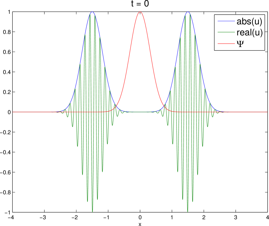
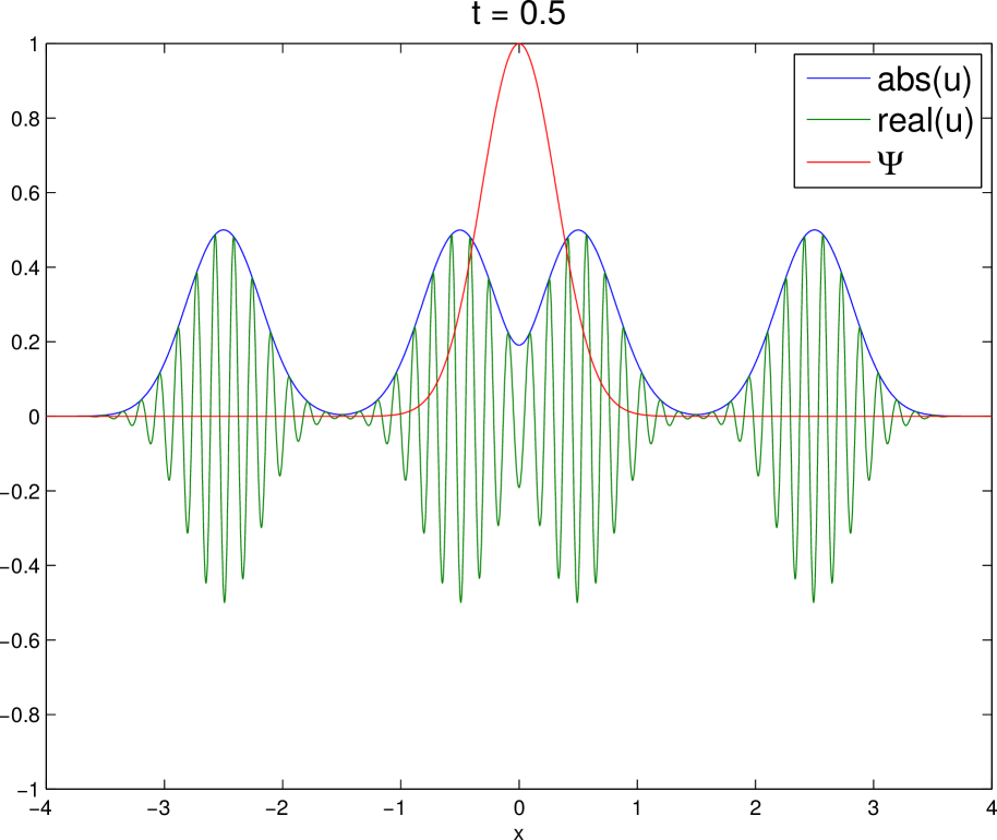
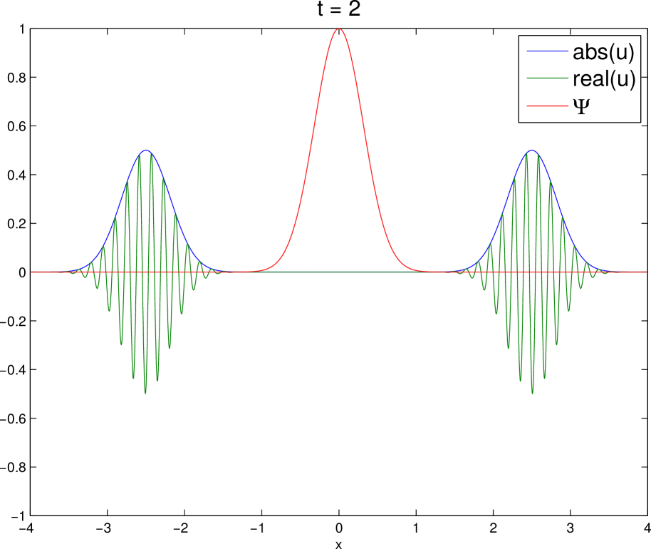
Figure 1: d’Alembert solution with initial data (25) and (28).

Let us consider a 1D case with spatially constant speed $c(x,y)=c(y)$. The initial data to (1),

$$u^{\varepsilon}(0,x,y)=B_{0}(x,y)e^{i\varphi_{0}(x,y)/\varepsilon},\qquad u_{t}^{\varepsilon}(0,x,y)=0,$$ (25)

generate the d’Alembert solution

$$u^{\varepsilon}(t,x,y)=u^{+}(t,x,y)+u^{-}(t,x,y),\qquad u^{\pm}(t,x,y)=\frac{1}{2}B_{0}(x\mp c(y)t,y)e^{i\varphi_{0}(x\mp c(y)t,y)/\varepsilon}.$$ (26)

The QoI (2) therefore reads

$$\widetilde{\mathcal{Q}}(t,y) =\int_{\mathbb{R}}|u^{+}(t,x,y)+u^{-}(t,x,y)|^{2}\psi(t,x)\,dx$$

$$=\int_{\mathbb{R}}\left(|u^{+}(t,x,y)|^{2}+|u^{-}(t,x,y)|^{2}+2\operatorname{Re}(u^{+}(t,x,y)^{*}u^{-}(t,x,y))\right)\psi(t,x)\,dx$$

$$=:\widetilde{Q}_{+}(t,y)+\widetilde{Q}_{-}(t,y)+\widetilde{Q}_{0}(t,y).$$ (27)

The first two terms of $\widetilde{\mathcal{Q}}$ yield

$$\widetilde{Q}_{\pm}(t,y)=\int_{\mathbb{R}}|u^{\pm}(t,x,y)|^{2}\psi(t,x)\,dx=\frac{1}{4}\int_{\mathbb{R}}B_{0}^{2}(x\mp c(y)t,y)\psi(t,x)\,dx,$$

where the integrand is smooth, compactly supported and independent of $\varepsilon$, including all its derivatives in $y$. Therefore, the terms $\widetilde{Q}_{\pm}$ satisfy Theorem 4.2. The last term $\widetilde{Q}_{0}$ reads

$$\widetilde{Q}_{0}(t,y)=\frac{1}{2}\int_{\mathbb{R}}\cos\left(\frac{\varphi(t,x,y)}{\varepsilon}\right)B_{0}(x+c(y)t,y)B_{0}(x-c(y)t,y)\psi(t,x)\,dx,$$

where $\varphi(t,x,y):=\varphi_{0}(x+c(y)t,y)-\varphi_{0}(x-c(y)t,y)$. This term could conceivably be problematic, depending on the choice of $B_{0}$ and $\varphi_{0}$. Notably, the selection

$$B_{0}(x,y)=e^{-5(x+s)^{2}}+e^{-5(x-s)^{2}},\qquad\varphi_{0}(x,y)=x,\qquad\psi(t,x)=e^{-5x^{2}},$$ (28)

produces two symmetric pulses centered at $\pm s$, each splitting into two waves traveling in opposite directions, see Figure 1 where we set $s=1.5$ and $c=2$. The test function $\psi$ is compactly supported in $x$ for numerical purposes. Let us also choose the speed $c(y)=y$ to be the stochastic variable. Then $\varphi(t,x,y)=2yt$ and $\widetilde{Q}_{0}$ includes an oscillatory prefactor $\cos\left({2yt}/{\varepsilon}\right)$ that does not depend on $x$ and hence cannot be damped by the test function $\psi$. Consequently, an $\varepsilon^{-\sigma}$ term is produced when differentiating $\partial_{y}^{\sigma}\widetilde{\mathcal{Q}}(t,y)$. Thus $\widetilde{\mathcal{Q}}$ does not satisfy Theorem 4.2. The QoI (2) along with its first and second derivative in $y$ is depicted in Figure 2, left column, for varying $\varepsilon=(1/40,1/80,1/160)$. The plots display oscillations of growing amplitude with increasing $\sigma$ and decreasing $\varepsilon$ as predicted. Here, we chose $y\in[1.5,2]$, $s=3$ and $t=2$.

In general, for odd-order polynomial $\varphi_{0}$, there is a cosine prefactor independent of $x$ in $\widetilde{Q}_{0}$ which induces oscillations in $\varepsilon$ of the QoI (2).

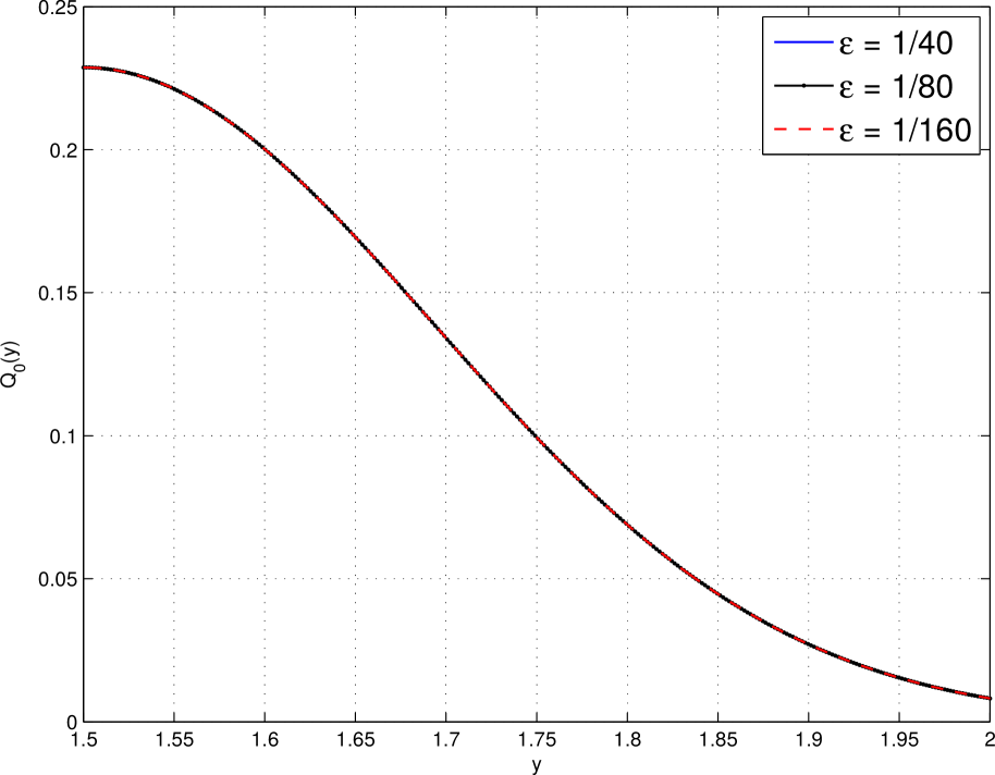
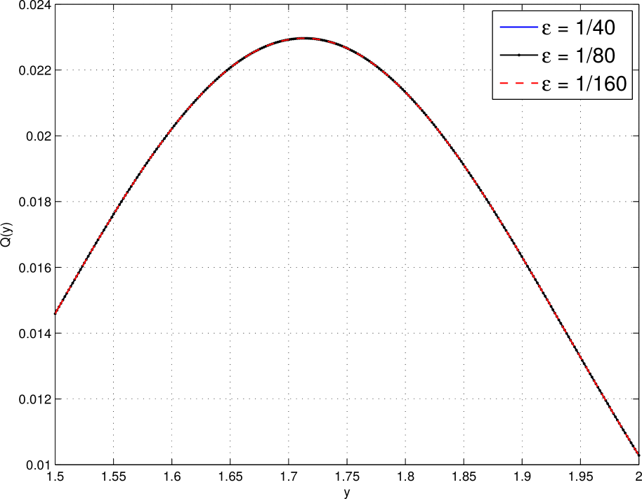
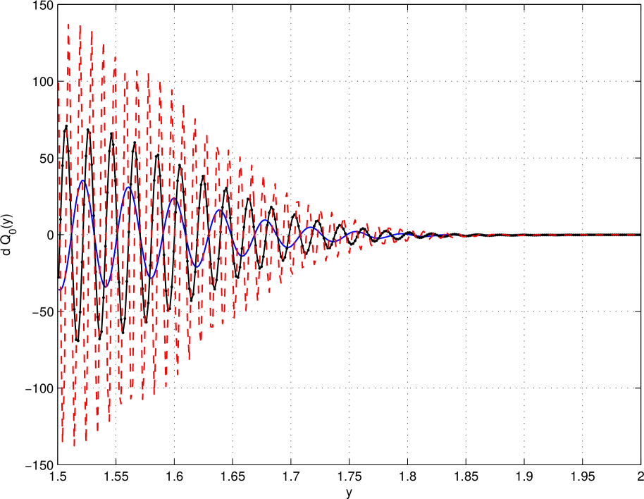
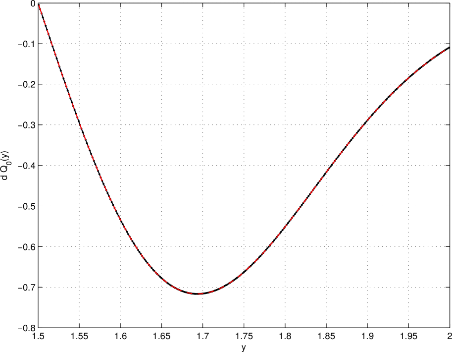
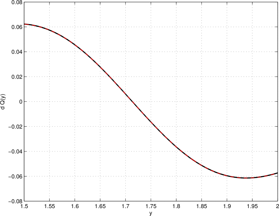
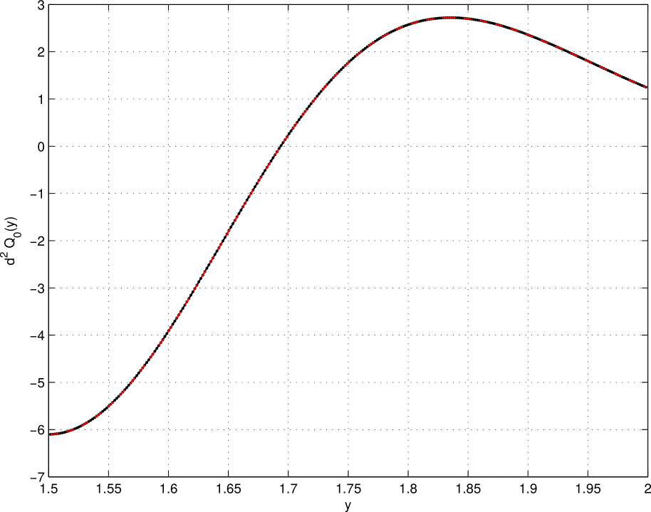
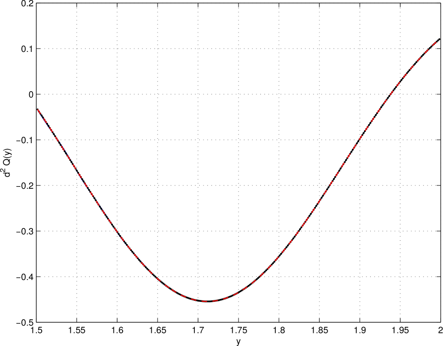
Figure 2: Left column: QoI (2) with $\varphi_{0}(x,y)=x$, and its first and second derivative in $y$. Central column: QoI (2) with $\varphi_{0}(x,y)=x^{2}$. Right column: QoI (4) with $\varphi_{0}(x,y)=x$.

Note that when $\varphi_{0}$ is an even-order polynomial in $x$, the QoI is not oscillatory for the example above. For instance, $\varphi_{0}(x,y)=x^{2}$ gives $\varphi(t,x,y)=4xyt$. By the non-stationary phase lemma, for all compact $\Gamma_{c}\subset\Gamma$ there exist $c_{s}$ independent of $\varepsilon$ such that

$$\sup_{\begin{subarray}{c}y\in\Gamma_{c}\\ t\in[0,T]\end{subarray}}\left|\int_{\mathbb{R}}\cos\left(\frac{4xyt}{\varepsilon}\right)B_{0}(x+yt,y)B_{0}(x-yt,y)\psi(x)\,dx\right|\leq c_{s}\varepsilon^{s},$$

for all $s$ as $\varepsilon\to 0$, and the same holds for its derivatives with respect to $y$. The QoI (2) with $\varphi_{0}(x,y)=x^{2}$ and its first and second derivatives in $y$ are plotted in Figure 2, central column, utilizing the same parameters as the previous example. No oscillations can be observed in the plot.

The different behavior of $\varphi_{0}(x,y)=x$ and $\varphi_{0}(x,y)=x^{2}$ in (28) does not come as a surprise if one looks at the GB approximation (19) of (2). Note that the left-going wave $u^{-}$ in (26) is approximated solely by $u_{k}^{-}$ in (12). This is because all GBs $v_{k}^{-}$ in (8) move along the rays $(q^{-},p^{-})$ whose initial data are $q^{-}(0,y,z)=z$ and $p^{-}(0,y,z)=1$ by (14). From (11) this implies that $p^{-}(t,y,z)=1$ and $q^{-}(t,y,z)=-yt+z$. Hence, as $y>0$ all $v_{k}^{-}$ move to the left. Similarly, $u^{+}$ is approximated merely by $u_{k}^{+}$. Therefore, the waves moving towards the origin (where the test function is supported) are from two different GB families. As stated above, a two-mode solution can thus give highly oscillatory QoIs.

In contrast, for $\varphi_{0}(x,y)=x^{2}$ we obtain $p^{\pm}(0,y,z)=p^{\pm}(t,y,z)=2z$ and hence $q^{\pm}(t,y,z)=\pm y\frac{z}{|z|}t+z$. Therefore, both $q^{+}$ and $q^{-}$ can move in either direction depending on the starting point $z$. For our example, this implies that the two waves moving towards the origin belong to the same GB mode, $u_{k}^{-}$, and the two waves moving away belong to $u_{k}^{+}$. Since the test function $\psi$ is compactly supported around the origin, only $u^{-}_{k}$ will substantially contribute to the QoI (19). Finally, by Theorem 4.3, the QoI (19) consisting of one GB mode solution is non-oscillatory.

Remark.

Generally, a phase $\varphi_{0}=\varphi_{0}(x)$ whose derivative changes sign on $\mathbb{R}$ allows for two waves approximated by the same mode moving in two different directions. In particular, this is true for even-order polynomials. Technically, $\varphi_{0}$ is not allowed to attain local extrema due to (A3). In practice however, it is enough to make sure that the support of $B_{0}$ and $B_{1}$ does not include the stationary point.

5.2 New quantity of interest

To avoid the oscillatory behavior of $\widetilde{\mathcal{Q}}$ in (27) we introduce the new QoI (4), in which $|u^{\varepsilon}|^{2}\psi$ is integrated not only in $\mathbf{x}$ but also in time $t$, with $\psi\in C^{\infty}_{c}(\mathbb{R}\times\mathbb{R}^{n})$. Let us first apply this QoI to the 1D oscillatory example from Section 5.1 with $\varphi_{0}(x,y)=x$,

$$\mathcal{Q}(y) =\int_{\mathbb{R}}\int_{\mathbb{R}}|u^{+}(t,x,y)+u^{-}(t,x,y)|^{2}\psi(t,x)\,dx\,dt,$$

$$=\int_{\mathbb{R}}\int_{\mathbb{R}}\left(|u^{+}(t,x,y)|^{2}+|u^{-}(t,x,y)|^{2}+2\operatorname{Re}(u^{+}(t,x,y)^{*}u^{-}(t,x,y))\right)\psi(t,x)\,dx\,dt$$

$$=:Q_{+}(y)+Q_{-}(y)+Q_{0}(y).$$

Again, the first two terms yield

$$Q_{\pm}(y)=\int_{\mathbb{R}}\int_{\mathbb{R}}|u^{\pm}(t,x,y)|^{2}\psi(t,x)\,dx\,dt=\frac{1}{4}\int_{\mathbb{R}}\int_{\mathbb{R}}B_{0}^{2}(x\mp yt,y)\psi(t,x)\,dx\,dt,$$

where the integrand is smooth, compactly supported in both $t$ and $x$ and independent of $\varepsilon$, including all its derivatives in $y$. The last term reads

$$Q_{0}(y)=\frac{1}{2}\int_{\mathbb{R}}\int_{\mathbb{R}}\cos\left(\frac{2yt}{\varepsilon}\right)B_{0}(x+yt,y)B_{0}(x-yt,y)\psi(t,x)\,dx\,dt,$$

and since the phase of $\cos\left(\frac{2yt}{\varepsilon}\right)$ has no stationary point in $t$, we can utilize the non-stationary phase lemma in $t$. As $\psi$ is compactly supported in both $t$ and $x$, we obtain the desired regularity: for all compact $\Gamma_{c}\subset\Gamma$, $\sup_{y\in\Gamma_{c}}|Q_{0}(y)|\leq c_{s}\varepsilon^{s}$ for all $s$ as $\varepsilon\to 0$, where $c_{s}$ is independent of $\varepsilon$ and similarly for differentiation in $y$. The same then holds for ${\mathcal{Q}}(y)$.

To confirm this numerically, we use the initial data from the previous section and set

$$\psi(t,x)=e^{-5x^{2}-300(t-t_{s})^{2}},$$

where $t_{s}=1.75$. The rightmost column of Figure 2 shows the QoI (4) and its first and second derivatives with respect to $y$ for $\varepsilon=(1/40,1/80,1/160)$. Compared to the first column the oscillations are eliminated.

5.3 Stochastic regularity of ${\mathcal{Q}}^{p,\boldsymbol{\alpha}}$

We now consider the general QoI $\mathcal{Q}^{p,\boldsymbol{\alpha}}$ in (3) with $\psi$ as in (A5) and define its GB approximated version as

$${\mathcal{Q}}^{p,\boldsymbol{\alpha}}_{\text{GB}}(\mathbf{y})=\varepsilon^{2(p+|\boldsymbol{\alpha}|)}\int_{\mathbb{R}}\int_{\mathbb{R}^{n}}g(t,\mathbf{x},\mathbf{y})|\partial_{t}^{p}\partial_{\mathbf{x}}^{\boldsymbol{\alpha}}u_{k}(t,\mathbf{x},\mathbf{y})|^{2}\psi(t,\mathbf{x})d\mathbf{x}\,dt.$$ (29)

We start off by defining the admissible cutoff parameter for the case of two-mode solutions.

Proposition 5.1.

Assume (A1)–(A3) hold. Then for all $T>0$, beam order $k$ and compact $\Gamma_{c}\subset\Gamma$, there is a GB cutoff width $\eta>0$ and constant $\delta>0$ such that for all $\mathbf{x}\in{\mathcal{B}}_{2\eta}$,

$$\operatorname{Im}\Phi_{k}^{\pm}(t,\mathbf{x},\mathbf{y},\mathbf{z})\geq\delta|\mathbf{x}|^{2},\quad\forall t\in[0,T],\,\mathbf{y}\in\Gamma_{c},\,\mathbf{z}\in K_{0}.$$ (30)

For the first order GB, $k=1$, we can take $\eta=\infty$ and (30) is valid for all ${\mathbf{x}}\in\mathbb{R}^{n}$.

Proof.

By Proposition 4.1, for every $\Gamma_{c}$ there exist $\delta^{+}>0$ and $\eta^{+}>0$ such that for all $\mathbf{x}\in{\mathcal{B}}_{2\eta^{+}}$ we have $\operatorname{Im}\Phi_{k}^{+}(t,\mathbf{x},\mathbf{y},\mathbf{z})\geq\delta^{+}|\mathbf{x}|^{2}$, and analogously for $\operatorname{Im}\Phi_{k}^{-}$ with $\delta^{-}$ and $\eta^{-}$. Then choosing $\delta=\min\{\delta^{+},\delta^{-}\}$ and $\eta=\min\{\eta^{+},\eta^{-}\}$ yields the relation (30) for all $\mathbf{x}\in{\mathcal{B}}_{2\eta}$. ∎

Definition 2.

The cutoff width $\eta$ used for the GB approximation is called admissible for a given $T$, $k$ and $\Gamma_{c}$ if it is small enough in the sense of Proposition 5.1.

Remark.

As in Section 4.1, we assume that $\eta<\infty$ without loss of generality. We note that also for the two-mode solutions, the Gaussian beam superposition (15) with no cutoff is identical to the one with a large enough cutoff, because of the compact support of the test function $\psi(t,\mathbf{x})$.

We will now prove the main theorem, which shows that the QoI (29) is indeed non-oscillatory.

Theorem 5.2.

Assume (A1)–(A5) hold. Moreover, let $\eta<\infty$ be admissible for $T>0$, $k$ and a compact $\Gamma_{c}\subset\Gamma$. Then for all $p\in{\mathbb{N}}$ and ${\boldsymbol{\alpha}}\in{\mathbb{N}_{0}^{N}}$, there exist $C_{\boldsymbol{\sigma}}$ such that

$$\sup_{\mathbf{y}\in\Gamma_{c}}\left|\frac{\partial^{\boldsymbol{\sigma}}{\mathcal{Q}}^{p,\boldsymbol{\alpha}}_{\text{GB}}(\mathbf{y})}{\partial\mathbf{y}^{\boldsymbol{\sigma}}}\right|\leq C_{\boldsymbol{\sigma}},\quad\forall\boldsymbol{\sigma}\in\mathbb{N}_{0}^{N},$$

where $C_{\boldsymbol{\sigma}}$ is independent of $\varepsilon$ but depends on $T$, $k$ and $\Gamma_{c}$.

In the proof we will use the following notation. Let $\mathcal{W}_{\mu}$ and $\Sigma_{\mu}$, for $\mu<\infty$, denote the spaces

$$\mathcal{W}_{\mu} =\Bigl{\{}f\in C^{\infty}:\text{supp}\,f(t,\cdot,\mathbf{y},\mathbf{z},\mathbf{z}^{\prime})\subset\Sigma_{\mu}(t,\mathbf{y},\mathbf{z},\mathbf{z}^{\prime}),\;\forall t\in\mathbb{R},\,\mathbf{y}\in\Gamma,\,\mathbf{z},\mathbf{z}^{\prime}\in\mathbb{R}^{n}\Bigr{\}},$$

$$\ \ \ \text{where}\>\Sigma_{\mu}(t,\mathbf{y},\mathbf{z},\mathbf{z}^{\prime}):=\{\mathbf{x}\in\mathbb{R}^{n}:|\mathbf{x}-\mathbf{q}^{+}(t,\mathbf{y},\mathbf{z})|\leq 2\mu\quad\text{and }\quad|\mathbf{x}-\mathbf{q}^{-}(t,\mathbf{y},\mathbf{z}^{\prime})|\leq 2\mu\}.$$

Note that the space $\Sigma_{\mu}$ is similar to $\Lambda_{\mu}$ introduced in Section 4.2. Instead of containing $\mathbf{x}$ that are close enough to two beams from the same mode, it contains $\mathbf{x}$ that lie at a distance at most $2\mu$ from two beams from different modes. We also note that there exist two spaces $\mathcal{S}^{\pm}_{\mu}$ as defined in Section 4.1 since we have two modes of $\Phi_{k}^{\pm}$ and that Lemma 4.4 holds for both.

For the remainder of the proof we fix the final time $T>0$, the beam order $k$ and the compact set $\Gamma_{c}\subset\Gamma$. Moreover, we select $\eta<\infty$ admissible in the sense of Definition 2. An important part of the proof relies on the non-stationary phase lemma:

Lemma 5.3 (Non-stationary phase lemma).

Suppose $\Theta\in C^{\infty}(\mathbb{R})$ and $f\in C_{c}^{\infty}(\mathbb{R})$ with $\text{supp}f\subset[0,T].$ If $\partial_{t}\Theta(t)\neq 0$ for all $t\in[0,T]$ then the following estimate holds true for all $K\in\mathbb{N}_{0}$,

$$\left|\int_{\mathbb{R}}f(t)e^{i\Theta(t)/\varepsilon}dt\right|\leq C_{K}(1+\|\Theta\|_{C^{K+1}([0,T])})^{K}\varepsilon^{K}\sum_{m\leq K}\int_{\mathbb{R}}\frac{|\partial_{t}^{m}f(t)|}{|\partial_{t}\Theta(t)|^{2K-m}}e^{-\operatorname{Im}\Theta(t)/\varepsilon}\,dt,$$

where $C_{K}$ depends on $K$ but is independent of $\varepsilon,f,\Theta$, $T$, and

$$\|\Theta\|_{C^{K+1}([0,T])}=\sum_{k=0}^{K+1}\sup_{t\in[0,T]}\left|\Theta^{(k)}(t)\right|.$$

The proof of this lemma is classical. See e.g. [13]. Upon keeping careful track of the constants in this proof we get the precise dependence on $\|\Theta\|$ in the right hand side of the estimate.

Lemma 5.4.

Define

$$I(\mathbf{y},\mathbf{u})=f(\mathbf{y},\mathbf{u})e^{i\Theta(\mathbf{y},\mathbf{u})/\varepsilon},$$

for $f,\Theta\in C^{\infty}(\Gamma\times\mathbb{R}^{d})$, where $\text{supp}\,f(\mathbf{y},\cdot)\subset D\subseteq\mathbb{R}^{d}$, $\forall\mathbf{y}\in\Gamma$. Then there exist functions $f_{j\boldsymbol{\sigma}}\in C^{\infty}(\Gamma\times\mathbb{R}^{d})$ with $\text{supp}\,f_{j\boldsymbol{\sigma}}(\mathbf{y},\cdot)\subset D$, $\forall\mathbf{y}\in\Gamma$ such that,

$$\frac{\partial^{\boldsymbol{\sigma}}I(\mathbf{y},\mathbf{u})}{\partial\mathbf{y}^{\boldsymbol{\sigma}}}=\sum_{j=0}^{|\boldsymbol{\sigma}|}\varepsilon^{-j}f_{j\boldsymbol{\sigma}}(\mathbf{y},\mathbf{u})e^{i\Theta(\mathbf{y},\mathbf{u})/\varepsilon}.$$ (31)

Proof.

We will carry out the proof by induction. For $\boldsymbol{\sigma}=\mathbf{0}$, we choose $f_{0\mathbf{0}}=f$ and the lemma holds. Let us assume (31) is true for a fixed $\boldsymbol{\sigma}$. Then for $\tilde{\boldsymbol{\sigma}}=\boldsymbol{\sigma}+\mathbf{e}_{k}$ where $\mathbf{e}_{k}$ is the $k$-th unit vector we have

$$\frac{\partial^{\tilde{\boldsymbol{\sigma}}}I(\mathbf{y},\mathbf{u})}{\partial\mathbf{y}^{\tilde{\boldsymbol{\sigma}}}} =\frac{\partial}{\partial y_{k}}\sum_{j=0}^{|\boldsymbol{\sigma}|}\varepsilon^{-j}f_{j\boldsymbol{\sigma}}(\mathbf{y},\mathbf{u})e^{i\Theta(\mathbf{y},\mathbf{u})/\varepsilon}$$

$$=\sum_{j=0}^{|\boldsymbol{\sigma}|}\varepsilon^{-j}\left(\frac{\partial f_{j\boldsymbol{\sigma}}(\mathbf{y},\mathbf{u})}{\partial y_{k}}+f_{j\boldsymbol{\sigma}}(\mathbf{y},\mathbf{u})\frac{i}{\varepsilon}\frac{\partial\Theta(\mathbf{y},\mathbf{u})}{\partial y_{k}}\right)e^{i\Theta(\mathbf{y},\mathbf{u})/\varepsilon}.$$

Hence we can take

$$f_{j\tilde{\boldsymbol{\sigma}}}=\left\{\begin{array}[]{ll}\frac{\partial f_{0\boldsymbol{\sigma}}}{\partial y_{k}},&j=0,\\ \frac{\partial f_{j\boldsymbol{\sigma}}}{\partial y_{k}}+if_{j-1\boldsymbol{\sigma}}\frac{\partial\Theta}{\partial y_{k}},&1\leq j\leq|\tilde{\boldsymbol{\sigma}}|-1,\\ if_{j-1\boldsymbol{\sigma}}\frac{\partial\Theta}{\partial y_{k}},&j=|\tilde{\boldsymbol{\sigma}}|.\end{array}\right.$$

Clearly, we have $f_{j\tilde{\boldsymbol{\sigma}}}\in C^{\infty}(\Gamma\times\mathbb{R}^{d})$ with $\text{supp}\,f_{j\tilde{\boldsymbol{\sigma}}}(\mathbf{y},\cdot)\subset D$ for all $\mathbf{y}\in\Gamma$. The proof is complete. ∎

Recalling the definition of $u_{k}$ in (15), $\mathcal{Q}^{p,\boldsymbol{\alpha}}_{\text{GB}}$ in (29) becomes

$$\mathcal{Q}^{p,\boldsymbol{\alpha}}_{\text{GB}}(\mathbf{y}) =\varepsilon^{2(p+|\boldsymbol{\alpha}|)}\int_{\mathbb{R}}\int_{\mathbb{R}^{n}}g(t,\mathbf{x},\mathbf{y})\left|\partial_{t}^{p}\partial_{\mathbf{x}}^{\boldsymbol{\alpha}}u^{+}_{k}(t,\mathbf{x},\mathbf{y})+\partial_{t}^{p}\partial_{\mathbf{x}}^{\boldsymbol{\alpha}}u^{-}_{k}(t,\mathbf{x},\mathbf{y})\right|^{2}\,\psi(t,\mathbf{x})d\mathbf{x}\,dt$$

$$=\varepsilon^{2(p+|\boldsymbol{\alpha}|)}\int_{\mathbb{R}}\int_{\mathbb{R}^{n}}g(t,\mathbf{x},\mathbf{y})[|\partial_{t}^{p}\partial_{\mathbf{x}}^{\boldsymbol{\alpha}}u^{+}_{k}(t,\mathbf{x},\mathbf{y})|^{2}+|\partial_{t}^{p}\partial_{\mathbf{x}}^{\boldsymbol{\alpha}}u^{-}_{k}(t,\mathbf{x},\mathbf{y})|^{2}$$

$$\qquad\qquad\qquad\qquad+2\operatorname{Re}(\partial_{t}^{p}\partial_{\mathbf{x}}^{\boldsymbol{\alpha}}u^{+}_{k}(t,\mathbf{x},\mathbf{y})^{*}\partial_{t}^{p}\partial_{\mathbf{x}}^{\boldsymbol{\alpha}}u^{-}_{k}(t,\mathbf{x},\mathbf{y}))]\,\psi(t,\mathbf{x})d\mathbf{x}\,dt$$

$$=:Q_{1}(\mathbf{y})+Q_{2}(\mathbf{y})+2\operatorname{Re}(Q_{3}(\mathbf{y})),$$ (32)

where $\psi\in C_{c}^{\infty}(\mathbb{R}\times\mathbb{R}^{n})$ is as in (A5) and $g\in C^{\infty}(\mathbb{R}\times\mathbb{R}^{n}\times\Gamma)$. The first two terms of (32), $Q_{1}$ and $Q_{2}$, possess the required stochastic regularity as a consequence of Theorem 4.2. Indeed, as $\psi$ is only supported for $t\in[0,T]$ we can write

$$Q_{1}(\mathbf{y})=\int_{0}^{T}\widetilde{Q}_{1}(t,{\mathbf{y}})dt,$$

where the reduced QoI $\tilde{Q}_{1}$ satisfies the assumptions of Theorem 4.2. (Note that when $\eta$ is admissible it admissible for both $\Phi_{k}^{+}$ and $\Phi_{k}^{-}$ individually.) Then

$$\sup_{\mathbf{y}\in\Gamma_{c}}\left|\partial_{\mathbf{y}}^{\boldsymbol{\sigma}}Q_{1}(\mathbf{y})\right|\leq\int_{0}^{T}\sup_{\begin{subarray}{c}\mathbf{y}\in\Gamma_{c}\\ t\in[0,T]\end{subarray}}\left|\partial_{\mathbf{y}}^{\boldsymbol{\sigma}}\widetilde{Q}_{1}^{p,\boldsymbol{\alpha}}(t,\mathbf{y})\right|\,dt\leq TC_{\boldsymbol{\sigma}},$$ (33)

and analogously for $Q_{2}$.

We will now prove that $Q_{3}$ satisfies the same regularity condition owing to the absence of stationary points of the phase. Let us examine the quantity

$$\partial_{\mathbf{y}}^{\boldsymbol{\sigma}}Q_{3}(\mathbf{y}) =\varepsilon^{2(p+|\boldsymbol{\alpha}|)}\partial_{\mathbf{y}}^{\boldsymbol{\sigma}}\int_{\mathbb{R}}\int_{\mathbb{R}^{n}}g(t,\mathbf{x},\mathbf{y})\partial_{t}^{p}\partial_{\mathbf{x}}^{\boldsymbol{\alpha}}u^{+}_{k}(t,\mathbf{x},\mathbf{y})^{*}\partial_{t}^{p}\partial_{\mathbf{x}}^{\boldsymbol{\alpha}}u^{-}_{k}(t,\mathbf{x},\mathbf{y})\,\psi(t,\mathbf{x})d\mathbf{x}\,dt$$

$$=\left(\frac{1}{2\pi\varepsilon}\right)^{n}\int_{K_{0}\times K_{0}}\int_{K_{1}}\partial^{\boldsymbol{\sigma}}_{\mathbf{y}}I(\mathbf{x},\mathbf{y},\mathbf{z},\mathbf{z}^{\prime})\,d\mathbf{x}\,d\mathbf{z}\,d\mathbf{z}^{\prime},$$ (34)

where

$$I(\mathbf{x},\mathbf{y},\mathbf{z},\mathbf{z}^{\prime})=\varepsilon^{2(p+|\boldsymbol{\alpha}|)}\int_{\mathbb{R}} \partial_{t}^{p}\partial_{\mathbf{x}}^{\boldsymbol{\alpha}}w_{k}^{+}(t,\mathbf{x}-\mathbf{q}^{+}(t,\mathbf{y},\mathbf{z}),\mathbf{y},\mathbf{z})^{*}\partial_{t}^{p}\partial_{\mathbf{x}}^{\boldsymbol{\alpha}}w_{k}^{-}(t,\mathbf{x}-\mathbf{q}^{-}(t,\mathbf{y},\mathbf{z}^{\prime}),\mathbf{y},\mathbf{z}^{\prime})$$

$$\times g(t,\mathbf{x},\mathbf{y})\psi(t,\mathbf{x})\,dt,$$

with

$$w_{k}^{\pm}(t,\mathbf{x},\mathbf{y},\mathbf{z})=A_{k}^{\pm}(t,\mathbf{x},\mathbf{y},\mathbf{z})\varrho_{\eta}(\mathbf{x})e^{i\Phi^{\pm}_{k}(t,\mathbf{x},\mathbf{y},\mathbf{z})/\varepsilon}.$$

Recalling Lemma 4.5, we can find $s_{k}^{\pm}\in\mathcal{S}_{\eta}^{\pm}$ such that

$$I(\mathbf{x},\mathbf{y},\mathbf{z},\mathbf{z}^{\prime}) =\int_{\mathbb{R}}s_{k}^{+}(t,\mathbf{x}-\mathbf{q}^{+}(t,\mathbf{y},\mathbf{z}),\mathbf{y},\mathbf{z})^{*}s_{k}^{-}(t,\mathbf{x}-\mathbf{q}^{-}(t,\mathbf{y},\mathbf{z}^{\prime}),\mathbf{y},\mathbf{z}^{\prime})g(t,\mathbf{x},\mathbf{y})\psi(t,\mathbf{x})\,dt$$

$$=\sum_{\ell=0}^{L_{1}}\sum_{m=0}^{L_{2}}\varepsilon^{\ell+m}\int_{\mathbb{R}}a_{\ell m}(t,\mathbf{x},\mathbf{y},\mathbf{z},\mathbf{z}^{\prime})\psi(t,\mathbf{x})e^{i\vartheta_{k}(t,\mathbf{x},\mathbf{y},\mathbf{z},\mathbf{z}^{\prime})/\varepsilon}\,dt,$$

where

$$a_{\ell m}(t,\mathbf{x},\mathbf{y},\mathbf{z},\mathbf{z}^{\prime})=g(t,\mathbf{x},\mathbf{y})p_{\ell}^{+}(t,\mathbf{x}-\mathbf{q}^{+}(t,\mathbf{y},\mathbf{z}),\mathbf{y},\mathbf{z})^{*}p_{m}^{-}(t,\mathbf{x}-\mathbf{q}^{-}(t,\mathbf{y},\mathbf{z}^{\prime}),\mathbf{y},\mathbf{z}^{\prime}),$$

with $p_{\ell}^{+},p_{m}^{-}\in\mathcal{P}_{\eta}$, and

$$\vartheta_{k}(t,\mathbf{x},\mathbf{y},\mathbf{z},\mathbf{z}^{\prime})=\Phi_{k}^{-}(t,\mathbf{x}-\mathbf{q}^{-}(t,\mathbf{y},\mathbf{z}^{\prime}),\mathbf{y},\mathbf{z}^{\prime})-\Phi_{k}^{+}(t,\mathbf{x}-\mathbf{q}^{+}(t,\mathbf{y},\mathbf{z}),\mathbf{y},\mathbf{z})^{*}.$$ (35)

By Proposition 3.1, we have $\vartheta_{k}\in C^{\infty}$, and $a_{\ell m}\in\mathcal{W}_{\eta}$ because both $p_{\ell}^{+},p_{m}^{-}$ are supported in the ball ${\mathcal{B}}_{2\eta}$. Therefore, by Lemma 5.4, there exist functions $f_{\ell mj\boldsymbol{\sigma}}\in\mathcal{W}_{\eta}$ such that

$$\partial_{\mathbf{y}}^{\boldsymbol{\sigma}}I(\mathbf{x},\mathbf{y},\mathbf{z},\mathbf{z}^{\prime})=\sum_{j=0}^{|\boldsymbol{\sigma}|}\sum_{\ell=0}^{L_{1}}\sum_{m=0}^{L_{2}}\varepsilon^{\ell+m-j}\int_{\mathbb{R}}f_{\ell mj\boldsymbol{\sigma}}(t,\mathbf{x},\mathbf{y},\mathbf{z},\mathbf{z}^{\prime})\psi(t,\mathbf{x})e^{i\vartheta_{k}(t,\mathbf{x},\mathbf{y},\mathbf{z},\mathbf{z}^{\prime})/\varepsilon}dt.$$ (36)

The following proposition shows that $\vartheta_{k}$ has no stationary points in $t\in[0,T]$ for all $\mathbf{x}\in\Sigma_{\mu}$ with a small enough $\mu$. Note that this is true even for $\mathbf{z}=\mathbf{z}^{\prime}$.

Proposition 5.5.

There exist $0<\mu\leq 1$ and $\nu>0$ such that for all $\mathbf{y}\in\Gamma_{c}$, $\mathbf{z}\in K_{0}$, $\mathbf{z}^{\prime}\in K_{0}$, $t\in[0,T]$ and for all $\mathbf{x}\in\Sigma_{\mu}$,

$$|\partial_{t}\vartheta_{k}(t,\mathbf{x},\mathbf{y},\mathbf{z},\mathbf{z}^{\prime})|\geq\nu.$$ (37)

Proof.

Differentiating (35) with respect to $t$ and using (9) and (11), we obtain

$$\partial_{t}\vartheta_{k}=-\partial_{t}\mathbf{q}^{-}\cdot\mathbf{p}^{-}+\partial_{t}\mathbf{q}^{+}\cdot\mathbf{p}^{+}+R_{k}=-c(\mathbf{q}^{-},\mathbf{y})|\mathbf{p}^{-}|-c(\mathbf{q}^{+},\mathbf{y})|\mathbf{p}^{+}|+R_{k},$$ (38)

where $R_{k}=R_{k}(t,\mathbf{x},\mathbf{y},\mathbf{z},\mathbf{z}^{\prime})$ reads

$$R_{k} =(\mathbf{x}-\mathbf{q}^{-})\cdot\partial_{t}\mathbf{p}^{-}-(\mathbf{x}-\mathbf{q}^{+})\cdot\partial_{t}\mathbf{p}^{+}-\partial_{t}\mathbf{q}^{-}\cdot M^{-}(\mathbf{x}-\mathbf{q}^{-})+\partial_{t}\mathbf{q}^{+}\cdot(M^{+})^{*}(\mathbf{x}-\mathbf{q}^{+})$$

$$+\frac{1}{2}(\mathbf{x}-\mathbf{q}^{-})\cdot\partial_{t}M^{-}(\mathbf{x}-\mathbf{q}^{-})+\frac{1}{2}(\mathbf{x}-\mathbf{q}^{+})\cdot(\partial_{t}M^{+})^{*}(\mathbf{x}-\mathbf{q}^{+})$$

$$+\sum_{|\boldsymbol{\beta}|=3}^{k+1}\frac{1}{\boldsymbol{\beta}!}\left(\partial_{t}\phi_{\boldsymbol{\beta}}^{-}(\mathbf{x}-\mathbf{q}^{-})^{\boldsymbol{\beta}}+\phi_{\boldsymbol{\beta}}^{-}\partial_{t}(\mathbf{x}-\mathbf{q}^{-})^{\boldsymbol{\beta}}\right)$$

$$-\sum_{|\boldsymbol{\beta}|=3}^{k+1}\frac{1}{\boldsymbol{\beta}!}\left(\partial_{t}\phi_{\boldsymbol{\beta}}^{+}(\mathbf{x}-\mathbf{q}^{+})^{\boldsymbol{\beta}}+\phi_{\boldsymbol{\beta}}^{+}\partial_{t}(\mathbf{x}-\mathbf{q}^{+})^{\boldsymbol{\beta}}\right)^{*}.$$

Since $\mathbf{q}^{\pm},\mathbf{p}^{\pm},M^{\pm},\phi_{\boldsymbol{\beta}}^{\pm}$ are smooth in all variables by Proposition 3.1, their time derivative is uniformly bounded in the compact set $[0,T]\times\Gamma_{c}\times K_{0}$. If $\mathbf{x}\in\Sigma_{\mu}$ for some $0<\mu\leq 1$, then both $|\mathbf{x}-\mathbf{q}^{-}|\leq 2\mu$ and $|\mathbf{x}-\mathbf{q}^{+}|\leq 2\mu$ and we arrive at

$$|R_{k}|\leq C_{k}\mu,$$

with $C_{k}$ independent of $\mu$.

Next, we note that $H(\mathbf{p}^{+},\mathbf{q}^{+},\mathbf{y})=c(\mathbf{q}^{+},\mathbf{y})|\mathbf{p}^{+}|$ is conserved along the ray,

$$c(\mathbf{q}^{+}(t,\mathbf{y},\mathbf{z}),\mathbf{y})|\mathbf{p}^{+}(t,\mathbf{y},\mathbf{z})|=c(\mathbf{q}^{+}(0,\mathbf{y},\mathbf{z}),\mathbf{y})|\mathbf{p}^{+}(0,\mathbf{y},\mathbf{z})|=c(\mathbf{z},\mathbf{y})|\nabla\varphi_{0}(\mathbf{z},\mathbf{y})|,$$

and therefore by (A1) and (A3) we obtain a uniform lower bound on $c(\mathbf{q}^{+},\mathbf{y})|\mathbf{p}^{+}|$, for all $t\in\mathbb{R}$, $\mathbf{y}\in\Gamma_{c}$ and $\mathbf{z}\in K_{0}$,

$$c(\mathbf{q}^{+}(t,\mathbf{y},\mathbf{z}),\mathbf{y})|\mathbf{p}^{+}(t,\mathbf{y},\mathbf{z})|\geq c_{\text{min}}\inf_{\begin{subarray}{c}\mathbf{z}\in K_{0}\\ \mathbf{y}\in\Gamma_{c}\end{subarray}}|\nabla\varphi_{0}(\mathbf{z},\mathbf{y})|\geq\gamma>0,$$

and similarly, from the conservation of $H(\mathbf{p}^{-},\mathbf{q}^{-},\mathbf{y})$ we obtain $c(\mathbf{q}^{-}(t,\mathbf{y},\mathbf{z}^{\prime}),\mathbf{y})|\mathbf{p}^{-}|\geq\gamma>0$. Thus from (38) we get

$$|\partial_{t}\vartheta_{k}|\geq c(\mathbf{q}^{-},\mathbf{y})|\mathbf{p}^{-}|+c(\mathbf{q}^{+},\mathbf{y})|\mathbf{p}^{+}|-|R_{k}|\geq 2\gamma-C_{k}\mu\geq\nu>0,$$

for all $\mathbf{x}\in\Sigma_{\mu}$ upon taking $\mu$ small enough. ∎

We are now ready to finalize the proof of Theorem 5.2. We first choose $0<\mu\leq\eta<\infty$ such that Proposition 5.5 holds. Furthermore, note that the admissibility condition implies that for all $\mathbf{x}$ satisfying $|\mathbf{x}-\mathbf{q}^{\pm}|\leq 2\eta$ we have $\operatorname{Im}\Phi_{k}^{\pm}(t,\mathbf{x}-\mathbf{q}^{\pm},\mathbf{y},\mathbf{z})\geq\delta|\mathbf{x}-\mathbf{q}^{\pm}|^{2}$. We can therefore estimate $\operatorname{Im}\vartheta_{k}$ with $\vartheta_{k}$ as in (35) as

$$\operatorname{Im}\vartheta_{k}(t,\mathbf{x},\mathbf{y},\mathbf{z},\mathbf{z}^{\prime}) =\operatorname{Im}\Phi_{k}^{-}(t,\mathbf{x}-\mathbf{q}^{-}(t,\mathbf{y},\mathbf{z}^{\prime}),\mathbf{y},\mathbf{z}^{\prime})+\operatorname{Im}\Phi_{k}^{+}(t,\mathbf{x}-\mathbf{q}^{+}(t,\mathbf{y},\mathbf{z}),\mathbf{y},\mathbf{z})$$

$$\geq\delta|\mathbf{x}-\mathbf{q}^{-}(t,\mathbf{y},\mathbf{z}^{\prime})|^{2}+\delta|\mathbf{x}-\mathbf{q}^{+}(t,\mathbf{y},\mathbf{z})|^{2},$$ (39)

for all $\mathbf{x}\in\Sigma_{\eta}$. To estimate $|\partial_{\mathbf{y}}^{\boldsymbol{\sigma}}Q_{3}|$ we recall (34),

$$\left|\partial_{\mathbf{y}}^{\boldsymbol{\sigma}}Q_{3}(\mathbf{y})\right|\leq\left(\frac{1}{2\pi\varepsilon}\right)^{n}\int_{K_{0}\times K_{0}}\int_{K_{1}}\left|\partial_{\mathbf{y}}^{\boldsymbol{\sigma}}I(\mathbf{x},\mathbf{y},\mathbf{z},\mathbf{z}^{\prime})\right|\,d\mathbf{x}\,d\mathbf{z}\,d\mathbf{z}^{\prime},$$ (40)

and by (36) and (A4) one has

$$\left|\partial_{\mathbf{y}}^{\boldsymbol{\sigma}}I(\mathbf{x},\mathbf{y},\mathbf{z},\mathbf{z}^{\prime})\right|\leq\sum_{j=0}^{|\boldsymbol{\sigma}|}\sum_{\ell=0}^{L_{1}}\sum_{m=0}^{L_{2}}\varepsilon^{-|\boldsymbol{\sigma}|}\left|\int_{\mathbb{R}}f_{\ell mj\boldsymbol{\sigma}}(t,\mathbf{x},\mathbf{y},\mathbf{z},\mathbf{z}^{\prime})\psi(t,\mathbf{x})e^{i\vartheta_{k}(t,\mathbf{x},\mathbf{y},\mathbf{z},\mathbf{z}^{\prime})/\varepsilon}\,dt\right|.$$ (41)

Let us introduce the function

$$g_{1}(t,\mathbf{x},\mathbf{y},\mathbf{z},\mathbf{z}^{\prime})=\varrho_{\mu}(\mathbf{x}-\mathbf{q}^{+}(t,\mathbf{y},\mathbf{z}))\varrho_{\mu}(\mathbf{x}-\mathbf{q}^{-}(t,\mathbf{y},\mathbf{z}^{\prime})),$$

so that $g_{1}\in\mathcal{W}_{\mu}$. Then for $g_{2}:=1-g_{1}\in C^{\infty}$ and $\text{supp }g_{2}(t,\cdot,\mathbf{y},\mathbf{z},\mathbf{z}^{\prime})\subset\mathbb{R}^{n}\setminus\Sigma_{\mu/2}$ for all $t,\mathbf{y},\mathbf{z},\mathbf{z}^{\prime}$. We will now regard (41) one term at a time, and use the partition of unity $1=g_{1}+g_{2}$,

$$\int_{\mathbb{R}}f_{\ell mj\boldsymbol{\sigma}}\psi e^{i\vartheta_{k}/\varepsilon}\,dt=\int_{\mathbb{R}}f_{\ell mj\boldsymbol{\sigma}}\psi(g_{1}+g_{2})e^{i\vartheta_{k}/\varepsilon}\,dt={\raisebox{-0.9pt}{1}⃝}+{\raisebox{-0.9pt}{2}⃝}.$$

Let us first estimate the term \raisebox{-0.9pt}{1}⃝. We have $\Sigma_{\mu/2}\subset\Sigma_{\eta}$ and therefore for $g_{\ell mj\boldsymbol{\sigma}}:=f_{\ell mj\boldsymbol{\sigma}}\psi g_{1}$ we have $\text{supp }g_{\ell mj\boldsymbol{\sigma}}(\cdot,\mathbf{x},\mathbf{y},\mathbf{z},\mathbf{z}^{\prime})\subset[0,T]$, $\forall\mathbf{x},\mathbf{y},\mathbf{z},\mathbf{z}^{\prime}$, and $\text{supp }g_{\ell mj\boldsymbol{\sigma}}(t,\cdot,\mathbf{y},\mathbf{z},\mathbf{z}^{\prime})\subset\Sigma_{\mu/2}(t,\mathbf{y},\mathbf{z},\mathbf{z}^{\prime})\cap K_{1}$, $\forall t,\mathbf{y},\mathbf{z},\mathbf{z}^{\prime}$. We now restrict $(t,{\mathbf{y}},{\mathbf{z}},{\mathbf{z}}^{\prime})$ to the compact set $[0,T]\times\Gamma_{c}\times K_{0}\times K_{0}$. Since the gradient $\partial_{t}\vartheta_{k}$ does not vanish for $\mathbf{x}\in\Sigma_{\mu/2}$ on this set by Proposition 5.5 we can employ the non-stationary phase Lemma 5.3,

$$|{\raisebox{-0.9pt}{1}⃝}| \leq\left|\int_{\mathbb{R}}g_{\ell mj\boldsymbol{\sigma}}(t,\mathbf{x},\mathbf{y},\mathbf{z},\mathbf{z}^{\prime})e^{i\vartheta_{k}(t,\mathbf{x},\mathbf{y},\mathbf{z},\mathbf{z}^{\prime})/\varepsilon}\,dt\right|$$

$$\leq C_{K}D_{K}\varepsilon^{K}\sum_{q=0}^{K}\int_{\mathbb{R}}\frac{|\partial_{t}^{q}g_{\ell mj\boldsymbol{\sigma}}(t,\mathbf{x},\mathbf{y},\mathbf{z},\mathbf{z}^{\prime})|}{|\partial_{t}\vartheta_{k}(t,\mathbf{x},\mathbf{y},\mathbf{z},\mathbf{z}^{\prime})|^{2K-q}}e^{-\operatorname{Im}\vartheta_{k}(t,\mathbf{x},\mathbf{y},\mathbf{z},\mathbf{z}^{\prime})/\varepsilon}\,dt,$$

for every $K\in\mathbb{N}_{0}$. Here, $C_{K}$ only depends on $K$ and

$$D_{K}=\left(1+\left\|\vartheta_{k}(\,\cdot\,,\mathbf{x},\mathbf{y},\mathbf{z},\mathbf{z}^{\prime})\right\|_{C^{K+1}([0,T])}\right)^{K}\leq\tilde{D}_{K},$$

since $\vartheta\in C^{\infty}$ and $(\mathbf{x},\mathbf{y},\mathbf{z},\mathbf{z}^{\prime})$ belongs to the compact set $K_{1}\times\Gamma_{c}\times K_{0}\times K_{0}$. Similarly, since $g_{\ell mj\boldsymbol{\sigma}}\in C^{\infty}$, its time derivatives are uniformly bounded: for all $t\in[0,T]$, $\mathbf{y}\in\Gamma_{c}$, $\mathbf{z},\mathbf{z}^{\prime}\in K_{0}$ and ${\mathbf{x}}\in K_{1}$,

$$|\partial_{t}^{q}g_{\ell mj\boldsymbol{\sigma}}(t,\mathbf{x},\mathbf{y},\mathbf{z},\mathbf{z}^{\prime})|\leq C_{\ell mj\boldsymbol{\sigma}q}.$$

Therefore, using the fact that $\operatorname{Im}\vartheta_{k}\geq 0$ from (39) and recalling (37) we obtain

$$|{\raisebox{-0.9pt}{1}⃝}|\leq C_{K}\varepsilon^{K}\sum_{q=0}^{K}\int_{0}^{T}\frac{C_{\ell mj\boldsymbol{\sigma}q}}{{\nu}^{2K-q}}\,dt\leq\widetilde{C}_{K\ell mj\boldsymbol{\sigma}}\varepsilon^{K},$$

where $\widetilde{C}_{K\ell mj\boldsymbol{\sigma}}$ also depends on $T,\mu,\eta,\Gamma_{c},k,\nu,p,\boldsymbol{\alpha}$, but is independent of $\varepsilon$.

Secondly, let us estimate the term \raisebox{-0.9pt}{2}⃝. Since $\text{supp }g_{2}(t,\cdot,\mathbf{y},\mathbf{z},\mathbf{z}^{\prime})\subset\mathbb{R}^{n}\setminus\Sigma_{\mu/2}(t,\mathbf{y},\mathbf{z},\mathbf{z}^{\prime})$, \raisebox{-0.9pt}{2}⃝ is only nonzero for either $|\mathbf{x}-\mathbf{q}^{+}(t,\mathbf{y},\mathbf{z})|>2\mu$ or $|\mathbf{x}-\mathbf{q}^{-}(t,\mathbf{y},\mathbf{z}^{\prime})|>2\mu$ (or both) and therefore by (39),

$$\operatorname{Im}\vartheta_{k}(t,\mathbf{x},\mathbf{y},\mathbf{z},\mathbf{z}^{\prime})\geq\delta\mu^{2},$$

whenever $t\in[0,T]$, $\mathbf{y}\in\Gamma_{c}$, $\mathbf{z},\mathbf{z}^{\prime}\in K_{0}$ and ${\mathbf{x}}$ is in the support of $g_{2}$. As $h_{\ell mj\boldsymbol{\sigma}}:=f_{\ell mj\boldsymbol{\sigma}}\psi g_{2}\in C^{\infty}$, \raisebox{-0.9pt}{2}⃝ can be estimated as

$$|{\raisebox{-0.9pt}{2}⃝}| \leq\int_{0}^{T}\left|h_{\ell mj\boldsymbol{\sigma}}(t,\mathbf{x},\mathbf{y},\mathbf{z},\mathbf{z}^{\prime})\right|e^{-\operatorname{Im}\vartheta_{k}(t,\mathbf{x},\mathbf{y},\mathbf{z},\mathbf{z}^{\prime})/\varepsilon}\,dt$$

$$\leq T\widetilde{C}_{\ell mj\boldsymbol{\sigma}}e^{-\delta\mu^{2}/\varepsilon},$$

for all $\mathbf{y}\in\Gamma_{c}$, $\mathbf{z},\mathbf{z}^{\prime}\in K_{0}$ and ${\mathbf{x}}\in K_{1}$. Collecting \raisebox{-0.9pt}{1}⃝ and \raisebox{-0.9pt}{2}⃝ together, we obtain from (41)

$$\left|\partial^{\boldsymbol{\sigma}}_{\mathbf{y}}I(\mathbf{x},\mathbf{y},\mathbf{z},\mathbf{z}^{\prime})\right| \leq\sum_{j=0}^{|\boldsymbol{\sigma}|}\sum_{\ell=0}^{L_{1}}\sum_{m=0}^{L_{2}}\varepsilon^{-|\boldsymbol{\sigma}|}\left(|{\raisebox{-0.9pt}{1}⃝}|+|{\raisebox{-0.9pt}{2}⃝}|\right)$$

$$\leq\max_{j,\ell,m}\varepsilon^{-|\boldsymbol{\sigma}|}\left(\widetilde{C}_{K\ell mj\boldsymbol{\sigma}}\varepsilon^{K}+T\widetilde{C}_{\ell mj\boldsymbol{\sigma}}e^{-\delta\mu^{2}/\varepsilon}\right).$$

Finally, by (40) we have

$$\left|\partial_{\mathbf{y}}^{\boldsymbol{\sigma}}Q_{3}(\mathbf{y})\right| \leq(2\pi)^{-n}\varepsilon^{-|\boldsymbol{\sigma}|-n}|K_{0}|^{2}|K_{1}|\max_{j,\ell,m}\left(\widetilde{C}_{K\ell mj\boldsymbol{\sigma}}\varepsilon^{K}+T\widetilde{C}_{\ell mj\boldsymbol{\sigma}}e^{-\delta\mu^{2}/\varepsilon}\right).$$

That is, choosing $K\geq n+|\boldsymbol{\sigma}|$, the first term is bounded in $\varepsilon$. Since $\delta>0$, the second term decays fast as a function of $\varepsilon$ for any $\boldsymbol{\sigma}$. Therefore, there exists an upper bound $C_{\boldsymbol{\sigma}}$ such that

$$\sup_{\mathbf{y}\in\Gamma_{c}}\left|\partial^{\boldsymbol{\sigma}}_{\mathbf{y}}Q_{3}(\mathbf{y})\right|\leq C_{\boldsymbol{\sigma}},$$

where $C_{\boldsymbol{\sigma}}$ depends on $T,\mu,\eta,\Gamma_{c},k,\delta,L_{1},L_{2},p,\boldsymbol{\alpha}$, but is uniform in $\varepsilon$. Recalling (32) and (33) we then arrive at

$$\sup_{\mathbf{y}\in\Gamma_{c}}\left|\partial_{\mathbf{y}}^{\boldsymbol{\sigma}}{\mathcal{Q}}_{\text{GB}}^{p,\boldsymbol{\alpha}}(\mathbf{y})\right|\leq\sup_{\mathbf{y}\in\Gamma_{c}}\left|\partial_{\mathbf{y}}^{\boldsymbol{\sigma}}Q_{1}(\mathbf{y})\right|+\sup_{\mathbf{y}\in\Gamma_{c}}\left|\partial_{\mathbf{y}}^{\boldsymbol{\sigma}}Q_{2}(\mathbf{y})\right|+2\sup_{\mathbf{y}\in\Gamma_{c}}\left|\partial_{\mathbf{y}}^{\boldsymbol{\sigma}}Q_{3}(\mathbf{y})\right|\leq\widetilde{C}_{\boldsymbol{\sigma}},$$

with $C_{\boldsymbol{\sigma}}$ dependent on $T,\mu,\eta,\Gamma_{c},k,K,\delta,\nu,L_{1},L_{2},p,\boldsymbol{\alpha}$, but independent of $\varepsilon$, which concludes the proof of Theorem 5.2.

5.4 Numerical example

A numerical example was presented in Section 5.1 comparing the QoIs $\widetilde{\mathcal{Q}}$ in (2) and $\mathcal{Q}$ in (4). We were able to obtain the exact solution since the speed was constant and the spatial variable was one-dimensional. In higher dimensions, however, caustics can appear and the exact solution is typically no longer available. Instead, we make use of the GB approximations $\widetilde{\mathcal{Q}}_{\text{GB}}$ in (19) and $\mathcal{Q}_{\text{GB}}:=\mathcal{Q}_{\text{GB}}^{0,\textbf{0}}$ in (16).

Let us consider a 2D wave equation (1) with $\mathbf{x}=[x_{1},x_{2}]$. The initial data include two random parameters $\mathbf{y}=[y_{1},y_{2}]$,

$$B_{0}(\mathbf{x},\mathbf{y}) =e^{-10((x_{1}+1)^{2}+(x_{2}-y_{1})^{2})}+e^{-10((x_{1}-1)^{2}+(x_{2}-y_{1})^{2})}, B_{1}(\mathbf{x},\mathbf{y})=0,$$

$$\varphi_{0}(\mathbf{x},\mathbf{y}) =|x_{1}|+(x_{2}-y_{1})^{2}, c(\mathbf{x},\mathbf{y})=y_{2}.$$

The test function is chosen as

$$\psi(\mathbf{x})=\left\{\begin{array}[]{ll}e^{-\frac{|\mathbf{x}|^{2}}{1-|\mathbf{x}|^{2}}},&\text{for }|\mathbf{x}|\leq 1,\\ 0,&\text{otherwise}.\end{array}\right.$$

This setup corresponds to two pulses centered in $(\pm 1,y_{1})$ at $t=0$, moving along the $x_{1}$ axis, while spreading or contracting in the $x_{2}$ direction, see Figure 3, where we plot the modulus of the first-order GB solution $|u_{1}(t,\mathbf{x},\mathbf{y})|$ at $t=1$ for various combinations of $y$. The central circle denotes the support of the test function $\psi$.

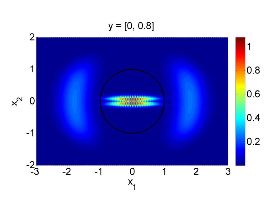
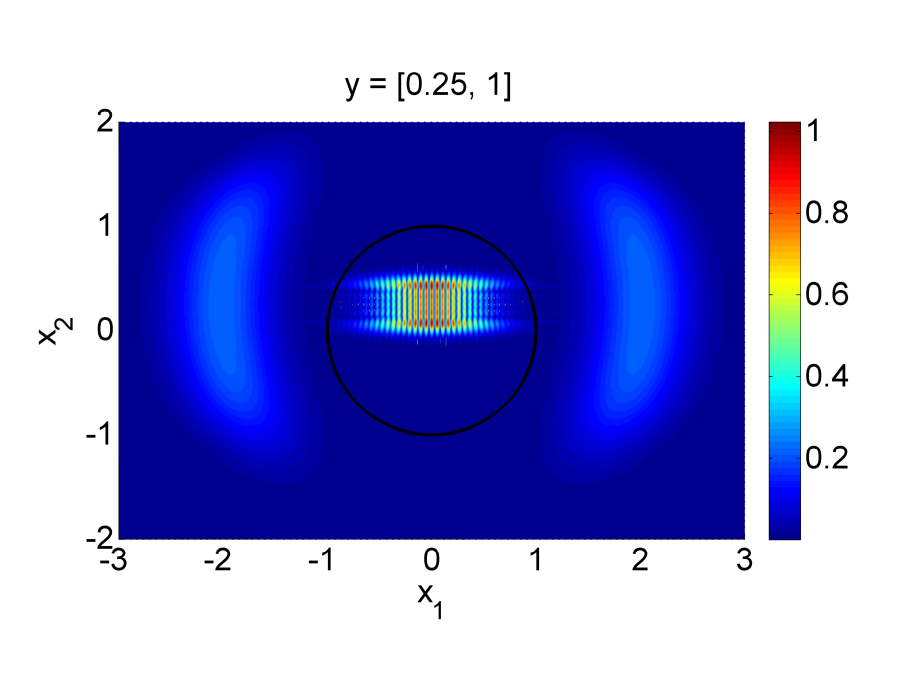
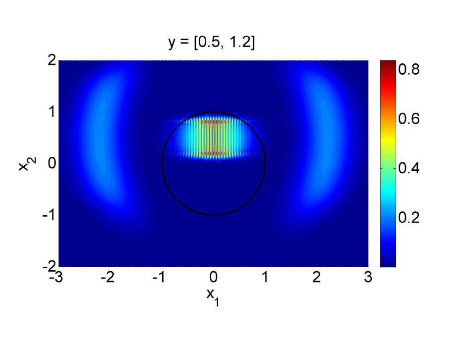
Figure 3: The modulus of the GB solution $|u_{1}(t,\mathbf{x},\mathbf{y})|$ for $\varepsilon=1/60$ and $\varphi_{0}(\mathbf{x},\mathbf{y})=|x_{1}|+(x_{2}-y_{1})^{2}$, at time $t=1$, for various $y$. The circle denotes the support of the test function $\psi$.

By analogous arguments as in Section 5.1, the part of the solution overlapping in the origin is from the same GB mode. Hence, the QoI $\widetilde{\mathcal{Q}}_{\text{GB}}$ with the test function supported around the origin should not oscillate. This is indeed the case, as seen in the left column of Figure 4, where the random variables are chosen as $y_{1}\in[0,0.5]$, $y_{2}\in[0.8,1.2]$ and we define $r\in[0,1]$, such that $[y_{1},y_{2}]=[0,0.8]+r[0.5,0.4]$ (i.e. the diagonal parameter). We plot $\widetilde{\mathcal{Q}}_{\text{GB}}$ and its first and second derivatives with respect to $r$ at time $t=1$ as a function of $r$.

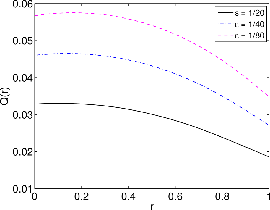
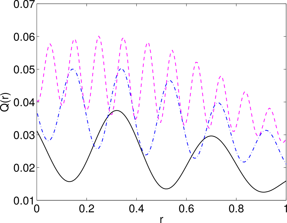
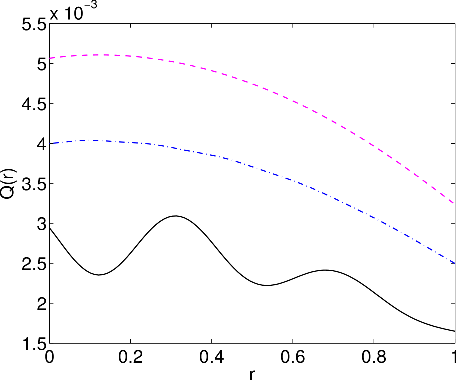
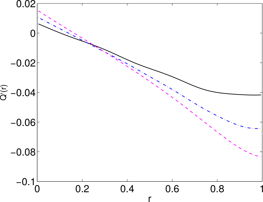
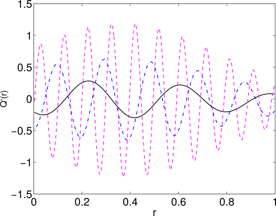
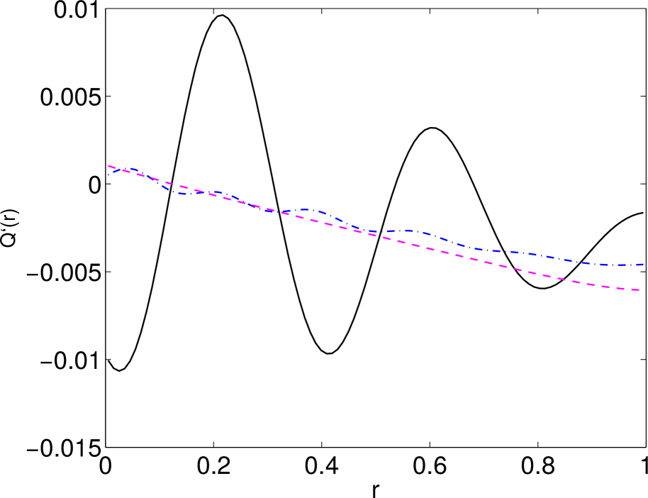
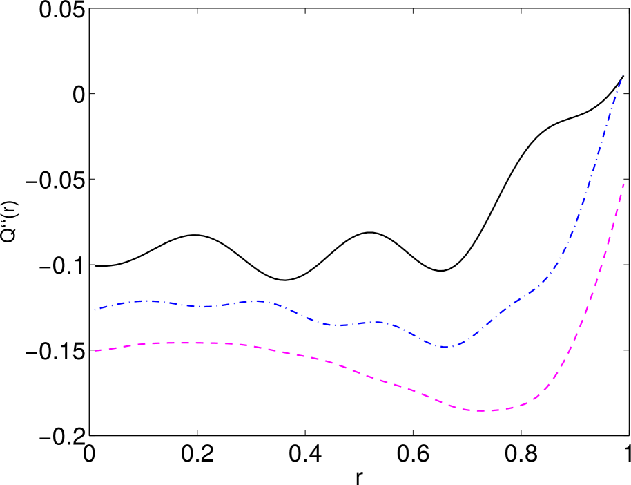
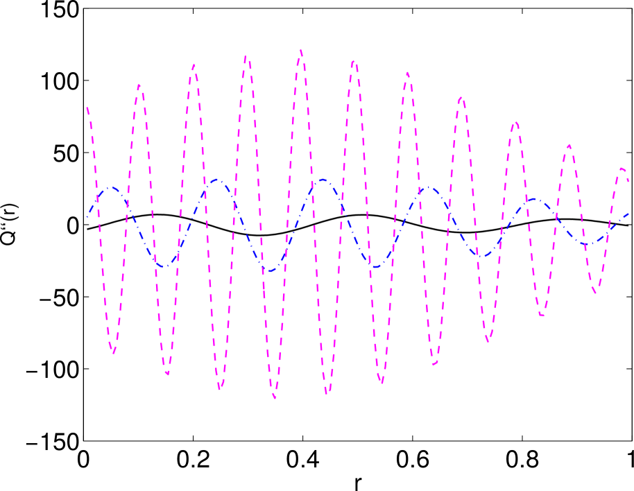
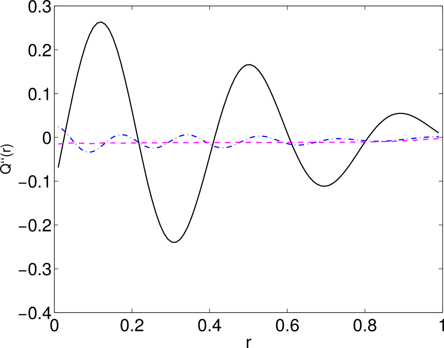
Figure 4: Left column: $\widetilde{\mathcal{Q}}_{\text{GB}}$ and its first and second derivatives for one-mode solution. Central column: $\widetilde{\mathcal{Q}}_{\text{GB}}$ and its first and second derivatives for two-mode solution. Right column: $\mathcal{Q}_{\text{GB}}$ and its first and second derivatives for two-mode solution.

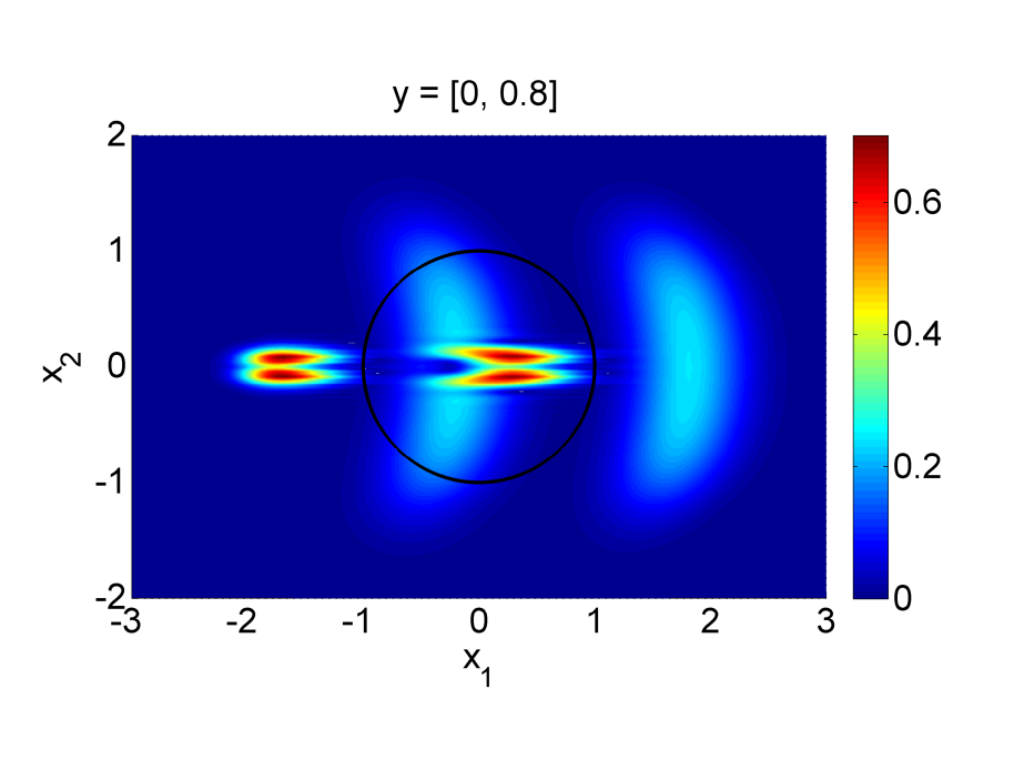
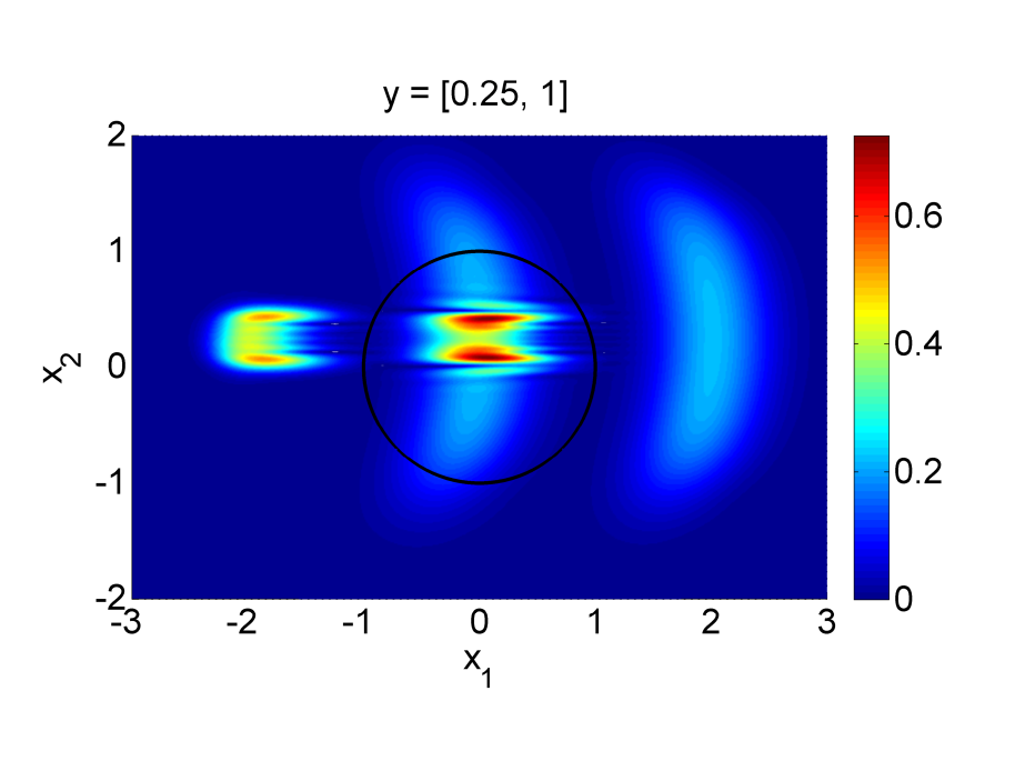
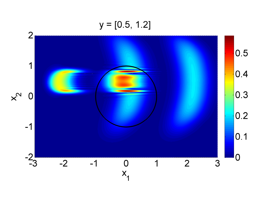
Figure 5: The modulus of the GB solution $|u_{1}(t,\mathbf{x},\mathbf{y})|$ for $\varepsilon=1/60$ and $\varphi_{0}(\mathbf{x},\mathbf{y})=x_{1}+(x_{2}-y_{1})^{2}$ at time $t=1$, for various $y$. The circle denotes the support of the test function $\psi$.

Let us now consider the same setup only changing the initial phase function to

$$\varphi_{0}(\mathbf{x},\mathbf{y})=x_{1}+(x_{2}-y_{1})^{2}.$$

Three realizations of $|u_{1}(t,\mathbf{x},\mathbf{y})|$ at $t=1$ are shown in Figure 5. It is no longer the case that the two branches moving towards the center can be described by the same GB mode. A numerical test plotted in Figure 4, central column, confirms the presence of two GB modes since the QoI cannot be bounded by a constant independent of $\varepsilon$. Here, we again plot $\widetilde{\mathcal{Q}}_{\text{GB}}$ and its first and second derivatives with respect to $r$ at time $t=1$ as a function of $r$. Oscillations with increasing amplitudes can be observed.

To get rid of the oscillations, we need to consider the time-integrated QoI $\mathcal{Q}_{\text{GB}}$. We introduce the test function

$$\psi(\mathbf{x})=\left\{\begin{array}[]{ll}e^{-\frac{|\mathbf{x}|^{2}}{1-|\mathbf{x}|^{2}}-10\frac{(t-1)^{2}}{0.2^{2}-(t-1)^{2}}},&\text{for }|\mathbf{x}|\leq 1,\text{and }|t-1|\leq 0.2,\\ 0,&\text{otherwise},\end{array}\right.$$

and integrate over both $\mathbf{x}$ and $t$. The QoI and its first and second derivatives are shown in Figure 4, right column. The oscillations do not disappear entirely, but their amplitude decrease rapidly as $\varepsilon\to 0$. This illustrates the difference between $\mathcal{Q}_{\text{GB}}$ and $\widetilde{\mathcal{Q}}_{\text{GB}}$.

Appendix A Proof of Theorem 4.6

To simplify the expressions, we first introduce the symmetrizing variables

$$\bar{\bf q}=\bar{\bf q}(t,\mathbb{y},\mathbf{z},\mathbf{z}^{\prime})=\frac{{\bf q}(t,\mathbb{y},\mathbf{z})+{\bf q}(t,\mathbb{y},\mathbf{z}^{\prime})}{2},\qquad\Delta{\bf q}=\Delta{\bf q}(t,\mathbb{y},\mathbf{z},\mathbf{z}^{\prime})=\frac{{\bf q}(t,\mathbb{y},\mathbf{z})-{\bf q}(t,\mathbb{y},\mathbf{z}^{\prime})}{2},$$ (42)

and the symmetrized version of the space ${\mathcal{T}}_{\eta}$ used in Section 4.2

$$\mathcal{T}^{s}_{\eta} :=\Bigl{\{}f\in C^{\infty}:\text{supp }f(t,\cdot,\mathbf{y},\mathbf{z},\mathbf{z}^{\prime})\subset\Lambda^{s}_{\eta}(t,\mathbf{y},\mathbf{z},\mathbf{z}^{\prime}),\>\forall t\in\mathbb{R},\,\mathbf{y}\in\Gamma,\,\mathbf{z},\mathbf{z}^{\prime}\in\mathbb{R}^{n}\Bigr{\}},$$

$$\ \ \ \text{where}\>\Lambda^{s}_{\eta}(t,\mathbf{y},\mathbf{z},\mathbf{z}^{\prime}):=\{\mathbf{x}\in\mathbb{R}^{n}:|\mathbf{x}-\Delta\mathbf{q}|\leq 2\eta\quad\text{and}\quad|\mathbf{x}+\Delta\mathbf{q}|\leq 2\eta\}.$$

Then $I_{0}$ in (24) can be written as

$$I_{0}(t,{\mathbf{y}},{\mathbf{z}},{\mathbf{z}}^{\prime})=\int_{\mathbb{R}^{n}}h(t,\mathbf{x},\mathbf{y},\mathbf{z},\mathbf{z}^{\prime})(\mathbf{x}-\Delta\mathbf{q})^{\boldsymbol{\alpha}}\>(\mathbf{x}+\Delta\mathbf{q})^{\boldsymbol{\beta}}\>e^{i\Psi_{k}(t,\mathbf{x},\mathbf{y},\mathbf{z},\mathbf{z}^{\prime})/\varepsilon}\,d\mathbf{x},$$ (43)

where $\Psi_{k}(t,\mathbf{x},\mathbf{y},\mathbf{z},\mathbf{z}^{\prime})=\Theta_{k}(t,\mathbf{x}+\bar{\mathbf{q}},\mathbf{y},\mathbf{z},\mathbf{z}^{\prime})$ and $h(t,\mathbf{x},\mathbf{y},\mathbf{z},\mathbf{z}^{\prime})=f(t,\mathbf{x}+\bar{\mathbf{q}},\mathbf{y},\mathbf{z},\mathbf{z}^{\prime})$ so that $h\in{\mathcal{T}}^{s}_{\eta}$ since $f\in\mathcal{T}_{\eta}$. The following auxiliary lemma is a compilation of Lemma 3 and the differentiated version of Lemma 4 in [23].

Lemma A.1.

There exists $f_{\boldsymbol{\mu},\boldsymbol{\nu}}\in C^{\infty}$ such that

$$(\mathbf{x}-\Delta\mathbf{q})^{\boldsymbol{\alpha}}\,(\mathbf{x}+\Delta\mathbf{q})^{\boldsymbol{\beta}}=\sum_{|\boldsymbol{\mu}+\boldsymbol{\nu}|=|\boldsymbol{\alpha}+\boldsymbol{\beta}|}f_{\boldsymbol{\mu},\boldsymbol{\nu}}(t,\mathbf{y},\mathbf{z},\mathbf{z}^{\prime})(\mathbf{z}-\mathbf{z}^{\prime})^{\boldsymbol{\mu}}\mathbf{x}^{\boldsymbol{\nu}}.$$

For the $k$-th order symmetrized Gaussian beam phase $\Psi_{k}$, there exist $a_{\boldsymbol{\alpha},\boldsymbol{\beta},m}\in C^{\infty}$ such that

$$\partial_{y_{m}}\Psi_{k}(t,\mathbf{x},\mathbf{y},\mathbf{z},\mathbf{z}^{\prime})=\sum_{2\leq|\boldsymbol{\alpha}+\boldsymbol{\beta}|\leq k+1}a_{\boldsymbol{\alpha},\boldsymbol{\beta},m}(t,\mathbf{y},\mathbf{z},\mathbf{z}^{\prime})\,(\mathbf{z}-\mathbf{z}^{\prime})^{\boldsymbol{\alpha}}\,\mathbf{x}^{\boldsymbol{\beta}}.$$

The following proposition is an update of [23, Proposition 3] adapted to our case.

Proposition A.2.

There exist functions $g_{\boldsymbol{\mu},\boldsymbol{\nu},\boldsymbol{\sigma},\ell}\in{\mathcal{T}}^{s}_{\eta}$ and $L_{\boldsymbol{\sigma}},M_{\boldsymbol{\sigma}}\geq 0$ such that the derivatives of $I_{0}$ in (43) with respect to $\mathbf{y}$ read

$$\partial^{\boldsymbol{\boldsymbol{\sigma}}}_{\mathbf{y}}I_{0}(t,\mathbf{y},\mathbf{z},\mathbf{z}^{\prime})=\sum_{\ell=-|\boldsymbol{\boldsymbol{\sigma}}|}^{L_{\boldsymbol{\sigma}}}\sum_{|\boldsymbol{\mu}+\boldsymbol{\nu}|+2\ell=0}^{M_{\boldsymbol{\sigma}}}\varepsilon^{\ell}(\mathbf{z}-\mathbf{z}^{\prime})^{\boldsymbol{\mu}}\int_{\mathbb{R}^{n}}\mathbf{x}^{\boldsymbol{\nu}}g_{\boldsymbol{\mu},\boldsymbol{\nu},\boldsymbol{\boldsymbol{\sigma}},\ell}(t,\mathbf{x},\mathbf{y},\mathbf{z},\mathbf{z}^{\prime})e^{i\Psi_{k}(t,\mathbf{x},\mathbf{y},\mathbf{z},\mathbf{z}^{\prime})/\varepsilon}d\mathbf{x}.$$ (44)

Proof.

Recalling Lemma A.1, (43) can be reformulated as

$$I_{0}(t,{\mathbf{y}},{\mathbf{z}},{\mathbf{z}}^{\prime})=\sum_{|\boldsymbol{\mu}+\boldsymbol{\nu}|=|\boldsymbol{\alpha}+\boldsymbol{\beta}|}(\mathbf{z}-\mathbf{z}^{\prime})^{\boldsymbol{\mu}}\int_{\mathbb{R}^{n}}\mathbf{x}^{\boldsymbol{\nu}}\>g_{\boldsymbol{\mu},\boldsymbol{\nu}}(t,\mathbf{x},\mathbf{y},\mathbf{z},\mathbf{z}^{\prime})\>e^{i\Psi_{k}(t,\mathbf{x},\mathbf{y},\mathbf{z},\mathbf{z}^{\prime})/\varepsilon}\,d\mathbf{x},$$

with $g_{\boldsymbol{\mu},\boldsymbol{\nu}}(t,\mathbf{x},\mathbf{y},\mathbf{z},\mathbf{z}^{\prime})=h(t,\mathbf{x},\mathbf{y},\mathbf{z},\mathbf{z}^{\prime})f_{\boldsymbol{\mu},\boldsymbol{\nu}}(t,\mathbf{y},\mathbf{z},\mathbf{z}^{\prime})$. Therefore, since $h\in\mathcal{T}^{s}_{\eta}$ and $f_{\boldsymbol{\mu},\boldsymbol{\nu}}\in C^{\infty}$ we have $g_{\boldsymbol{\mu},\boldsymbol{\nu}}\in{\mathcal{T}}^{s}_{\eta}$. We will now prove (44) by induction. First, the statement is valid for $\boldsymbol{\sigma}=\mathbf{0}$ since we can choose $L_{\boldsymbol{0}}=0$, $M_{\boldsymbol{0}}=|\boldsymbol{\alpha}+\boldsymbol{\beta}|$ and

$$g_{\boldsymbol{\mu},\boldsymbol{\nu},\mathbf{0},0}=\left\{\begin{array}[]{ll}g_{\boldsymbol{\mu},\boldsymbol{\nu}},&\text{for }|\boldsymbol{\mu}+\boldsymbol{\nu}|=|\boldsymbol{\alpha}+\boldsymbol{\beta}|,\\ 0,&\text{otherwise}.\end{array}\right.$$

For the induction step let $L_{\boldsymbol{\sigma}},M_{\boldsymbol{\sigma}}\geq 0$ and $g_{\boldsymbol{\mu},\boldsymbol{\nu},\boldsymbol{\sigma},\ell}\in{\mathcal{T}}^{s}_{\eta}$ be such that (44) holds. Then for $\tilde{\boldsymbol{\sigma}}=\boldsymbol{\sigma}+\mathbf{e}_{m},$ where $\mathbf{e}_{m}$ is the $m$-th unit vector, we have $\partial^{\tilde{\boldsymbol{\sigma}}}_{\mathbf{y}}I_{0}=\partial_{y_{m}}\partial_{\mathbf{y}}^{\boldsymbol{\sigma}}I_{0}$. Using (44), we can write

$$\partial^{\tilde{\boldsymbol{\sigma}}}_{\mathbf{y}}I_{0} =\sum_{\ell=-|\boldsymbol{\boldsymbol{\sigma}}|}^{L_{\boldsymbol{\sigma}}}\sum_{|\boldsymbol{\mu}+\boldsymbol{\nu}|+2\ell=0}^{M_{\boldsymbol{\sigma}}}\varepsilon^{\ell}(\mathbf{z}-\mathbf{z}^{\prime})^{\boldsymbol{\mu}}\int_{\mathbb{R}^{n}}\mathbf{x}^{\boldsymbol{\nu}}\left(\partial_{y_{m}}g_{\boldsymbol{\mu},\boldsymbol{\nu},\boldsymbol{\boldsymbol{\sigma}},\ell}+g_{\boldsymbol{\mu},\boldsymbol{\nu},\boldsymbol{\boldsymbol{\sigma}},\ell}\,i\varepsilon^{-1}\partial_{y_{m}}\Psi_{k}\right)\,e^{i\Psi_{k}/\varepsilon}d\mathbf{x}$$

$$={\raisebox{-0.9pt}{1}⃝}+{\raisebox{-0.9pt}{2}⃝}.$$

Since $\partial_{y_{m}}g_{\boldsymbol{\mu},\boldsymbol{\nu},\boldsymbol{\sigma},\ell}\in{\mathcal{T}}^{s}_{\eta}$, \raisebox{-0.9pt}{1}⃝ is of the form (44) with $L_{\tilde{\boldsymbol{\sigma}}}=L_{\boldsymbol{\sigma}}$, $M_{\tilde{\boldsymbol{\sigma}}}=M_{\boldsymbol{\sigma}}$ and

$$g_{\boldsymbol{\mu},\boldsymbol{\nu},\tilde{\boldsymbol{\sigma}},\ell}=\left\{\begin{array}[]{ll}\partial_{y_{m}}g_{\boldsymbol{\mu},\boldsymbol{\nu},\boldsymbol{\sigma},\ell},&\text{for }\ell\geq-|\boldsymbol{\sigma}|,\\ 0,&\text{for }\ell=-|\boldsymbol{\sigma}|-1.\end{array}\right.$$

Regarding the remaining terms \raisebox{-0.9pt}{2}⃝, let us express the derivative $\partial_{y_{m}}\Psi_{k}$ by Lemma A.1. Then \raisebox{-0.9pt}{2}⃝ reads

$$\sum_{\ell=-|\boldsymbol{\boldsymbol{\sigma}}|}^{L_{\boldsymbol{\sigma}}}\sum_{|\boldsymbol{\mu}+\boldsymbol{\nu}|+2\ell=0}^{M_{\boldsymbol{\sigma}}}\sum_{|\boldsymbol{\gamma}+\boldsymbol{\delta}|=2}^{k+1}\varepsilon^{\ell-1}(\mathbf{z}-\mathbf{z}^{\prime})^{\boldsymbol{\mu}+\boldsymbol{\gamma}}\int_{\mathbb{R}^{n}}\mathbf{x}^{\boldsymbol{\nu}+\boldsymbol{\delta}}h_{\boldsymbol{\mu},\boldsymbol{\nu},\boldsymbol{\gamma},\boldsymbol{\delta},\ell}\,e^{i\Psi_{k}/\varepsilon}d\mathbf{x},$$ (45)

with $h_{\boldsymbol{\mu},\boldsymbol{\nu},\boldsymbol{\gamma},\boldsymbol{\delta},\ell}=ia_{\boldsymbol{\gamma},\boldsymbol{\delta},m}\,g_{\boldsymbol{\mu},\boldsymbol{\nu},\boldsymbol{\boldsymbol{\sigma}},\ell}\in{\mathcal{T}}^{s}_{\eta}$ since $g_{\boldsymbol{\mu},\boldsymbol{\nu},\boldsymbol{\boldsymbol{\sigma}},\ell}\in\mathcal{T}^{s}_{\eta}$ and $a_{\boldsymbol{\gamma},\boldsymbol{\delta},m}\in C^{\infty}$. Each of the terms in (45) is therefore of the form

$$\varepsilon^{\tilde{\ell}}(\mathbf{z}-\mathbf{z}^{\prime})^{\tilde{\boldsymbol{\mu}}}\int_{\mathbb{R}^{n}}\mathbf{x}^{\tilde{\boldsymbol{\nu}}}h_{\tilde{\boldsymbol{\mu}},\tilde{\boldsymbol{\nu}},\tilde{\ell}}(t,\mathbf{x},\mathbf{y},\mathbf{z},\mathbf{z}^{\prime})\,e^{i\Psi_{k}(t,\mathbf{x},\mathbf{y},\mathbf{z},\mathbf{z}^{\prime})/\varepsilon}d\mathbf{x},$$

where

$$-|\tilde{\boldsymbol{\sigma}}|\leq\tilde{\ell}=\ell-1\leq L_{\boldsymbol{\sigma}}-1=:L_{\tilde{\boldsymbol{\sigma}}},$$

and

$$0\leq|\tilde{\boldsymbol{\mu}}+\tilde{\boldsymbol{\nu}}|+2\tilde{\ell}=|\boldsymbol{\mu}+\boldsymbol{\nu}|+2\ell+|\boldsymbol{\gamma}+\boldsymbol{\delta}|-2\leq M_{\boldsymbol{\sigma}}+k-1=:M_{\tilde{\boldsymbol{\sigma}}},$$

which finalizes the induction argument and concludes Proposition A.2. ∎

The rest of the proof of [23, Theorem 1] can be used as it is. In particular, if $\eta<\infty$, then [23, Lemma 5] and [23, Lemma 6] are valid without any alteration. Ultimately, we are using the fact that $0\leq|\boldsymbol{\mu}+\boldsymbol{\nu}|+2\ell$ in (44) which is still the case due to Proposition A.2. Finally, since all estimates in [23] are uniform in $t$, the constant $C_{\boldsymbol{\sigma}}$ is uniform in $[0,T]$ as well. This completes the proof of Theorem 4.6.

References

- [1] I. Babuska, F. Nobile, and R. Tempone. A stochastic collocation method for elliptic partial differential equations with random input data. SIAM Rev., 52:317–355, 2010.
- [2] I. Babuska, R. Tempone, and G. E. Zouraris. Solving elliptic boundary value problems with uncertain coefficients by the finite element method: the stochastic formulation. Comput. Method. Appl. M., 194:1251–1294, 2005.
- [3] I. M. Babuska, F. Nobile, and R. Tempone. A stochastic collocation method for elliptic partial differential equations with random input data. SIAM J. Numer. Anal., 45:1005–1034, 2007.
- [4] A. Bamberger, B. Engquist, L. Halpern, and P. Joly. Parabolic wave equation approximations in heterogeneous media. SIAM J. Appl. Math., 48(1):99–128, 1988.
- [5] H.-J. Bungartz and M. Griebel. Sparse grids. Acta Numer., 13:147–269, 2004.
- [6] V. Cervený, M. M. Popov, and I. Pšenčík. Computation of wave fields in inhomogeneous media — Gaussian beam approach. Geophys. J. R. Astr. Soc., 70:109–128, 1982.
- [7] A. Cohen, R. Devore, and C. Schwab. Analytic regularity and polynomial approximation of parametric and stochastic elliptic PDEs. Anal. Appl., 9:11–47, 2011.
- [8] B. Engquist and O. Runborg. Computational high frequency wave propagation. Acta Numer., 12:181–266, 2003.
- [9] G. S. Fishman. Monte Carlo: Concepts, Algorithms, and Applications. Springer- Verlag, New York, 1996.
- [10] R. G. Ghanem and P. D. Spanos. Stochastic finite elements: A spectral approach. Springer, New York, 1991.
- [11] M. Griebel and S. Knapek. Optimized general sparse grid approximation spaces for operator equations. Math. Comp., 78:2223–2257, 2009.
- [12] Robert J Hansen. Seismic design for nuclear power plants. The MIT Press, Cambridge, 1970.
- [13] L. Hörmander. The Analysis of Linear Partial Differential Operators I: Distribution Theory and Fourier Analysis. Springer-Verlag, 1983.
- [14] S. Jin, J.-G. Liu, and Z. Ma. Uniform spectral convergence of the stochastic Galerkin method for the linear transport equations with random inputs in diffusive regime and a micro-macro decomposition based asymptotic preserving method. Res. Math. Sci., 4(15), 2017.
- [15] S. Jin, L. Liu, G. Russo, and Z. Zhou. Gaussian wave packet transform based numerical scheme for the semi-classical Schrödinger equation with random inputs. Technical report, arXiv:1903.08740 [math.NA], 2019.
- [16] S. Jin and Y. Zhu. Hypocoercivity and uniform regularity for the Vlasov-Poisson Fokker–Planck system with uncertainty and multiple scales. SIAM J. Math. Anal., 50:1790–1816, 2018.
- [17] J. Li, Z. Fang, and G. Lin. Regularity analysis of metamaterial Maxwell’s equations with random coefficients and initial conditions. Comput. Method. Appl. M., 335:24–51, 2018.
- [18] Q. Li and L. Wang. Uniform regularity for linear kinetic equations with random input based on hypocoercivity. SIAM/ASA J. Uncertainty Quantification, 5(1):1193–1219, 2017.
- [19] H. Liu, O. Runborg, and N. M. Tanushev. Error estimates for Gaussian beam superpositions. Math. Comp., 82:919–952, 2013.
- [20] H. Liu, O. Runborg, and N. M. Tanushev. Sobolev and max norm error estimates for Gaussian beam superpositions. Commun. Math. Sci., 14(7):2037–2072, 2016.
- [21] L. Liu and S. Jin. Hypocoercivity based sensitivity analysis and spectral convergence of the stochastic Galerkin approximation to collisional kinetic equations with multiple scales and random inputs. Multiscale Model. Simul., 16(3):1085–1114, 2017.
- [22] G. Malenová. Uncertainty quantification for high frequency waves. Licentite thesis, KTH Royal Institute of Technology, 2016.
- [23] G. Malenová, M. Motamed, and O. Runborg. Stochastic regularity of a quadratic observable of high-frequency waves. Res. Math. Sci., 4(1):1–23, 2017.
- [24] G. Malenová, M. Motamed, O. Runborg, and R. Tempone. A sparse stochastic collocation technique for high-frequency wave propagation with uncertainty. SIAM/ASA J. Uncertainty Quantification, 4(1):1084–1110, 2016.
- [25] M. Motamed, F. Nobile, and R. Tempone. A stochastic collocation method for the second order wave equation with a discontinuous random speed. Num. Math., 123(3):495–546, 2013.
- [26] F. Nobile and R. Tempone. Analysis and implementation issues for the numerical approximation of parabolic equations with random coefficients. IJNME, 80:979–1006, 2009.
- [27] F. Nobile, R. Tempone, and C. G. Webster. A sparse grid stochastic collocation method for partial differential equations with random input data. SIAM J. Numer. Anal., 46:2309–2345, 2008.
- [28] J. Ralston. Gaussian beams and the propagation of singularities. Studies in partial differential equations, 23:206–248, 1982.
- [29] O. Runborg. Mathematical models and numerical methods for high frequency waves. Commun. Comput. Phys., 2:827–880, 2007.
- [30] R. W. Shu and S. Jin. Uniform regularity in the random space and spectral accuracy of the stochastic Galerkin method for a kinetic-fluid two-phase flow model with random initial inputs in the light particle regime. M2AN, 52:1651–1678, 2018.
- [31] N. M. Tanushev. Superpositions and higher order Gaussian beams. Commun. Math. Sci., 6(2):449–475, 2008.
- [32] R. A. Todor and C. Schwab. Convergence rates for sparse chaos approximations of elliptic problems with stochastic coefficients. IMA J. Numer. Anal., 27:232–261, 2007.
- [33] D. Xiu and J. S. Hesthaven. High-order collocation methods for differential equations with random inputs. SIAM J. Sci. Comput., 27:1118–1139, 2005.
- [34] D. Xiu and G. E. Karniadakis. Modeling uncertainty in steady state diffusion problems via generalized polynomial chaos. Comput. Method. Appl. M., 191:4927–4948, 2002.