Outer Approximation Methods for Solving Variational Inequalities Defined over the Solution Set of a Split Convex Feasibility Problem

Abstract

We study variational inequalities which are governed by a strongly monotone and Lipschitz continuous operator $F$ over a closed and convex set $S$. We assume that $S=C\cap A^{-1}(Q)$ is the nonempty solution set of a (multiple-set) split convex feasibility problem, where $C$ and $Q$ are both closed and convex subsets of two real Hilbert spaces $\mathcal{H}_{1}$ and $\mathcal{H}_{2}$, respectively, and the operator $A$ acting between them is linear. We consider a modification of the gradient projection method the main idea of which is to replace at each step the metric projection onto $S$ by another metric projection onto a half-space which contains $S$. We propose three variants of a method for constructing the above-mentioned half-spaces by employing the multiple-set and the split structure of the set $S$. For the split part we make use of the Landweber transform.

Keywords: $CQ$-method, split convex feasibility problem, variational inequality.

AMS Subject Classification: 47H09, 47H10, 47J20, 47J25, 65K15.

1 Introduction

Let $\mathcal{H}_{1}$ and $\mathcal{H}_{2}$ be two real Hilbert spaces. In this paper we consider the following variational inequality problem (VI($F$, $S$)) governed by an $L$-Lipschitz continuous and $\alpha$-strongly monotone operator $F\colon\mathcal{H}_{1}\rightarrow\mathcal{H}_{1}$ over a nonempty, closed and convex subset $S\subseteq\mathcal{H}_{1}$: find a point $x^{*}\in S$ for which the inequality

$$\langle Fx^{*},z-x^{*}\rangle\geq 0$$ (1.1)

holds true for all $z\in S$.

It is well known that the gradient projection method [25]

$$u_{0}\in\mathcal{H}_{1},\qquad u_{k+1}:=P_{S}(u_{k}-\lambda F(u_{k})),\qquad k=0,1,2,\ldots,$$ (1.2)

generates a sequence which converges in norm to the unique solution of VI($F$, $S$) when $\lambda\in(0,\frac{2\alpha}{L^{2}})$. This is due to the fact that the operator $P_{S}(\operatorname*{Id}-\lambda F)$ becomes a strict contraction the fixed point of which coincides with the solution of VI($F$, $S$); see [41, Theorem 46.C] or [16, Theorem 5].

Gibali et al. [24] have proposed the framework of outer approximation methods, where the unknown parameter $\lambda$ is replaced by a null, non-summable sequence $\{\lambda_{k}\}_{k=0}^{\infty}\subseteq[0,\infty)$ and the difficult projection onto $S$ is replaced by a sequence of simpler to evaluate metric projections onto certain half-spaces $H_{k}\supseteq S$. The computational cost of such methods depends to a large extent on the construction of the half-spaces $H_{k}$ which, in [24], were obtained by using a given sequence of cutter operators (see Definition 2.3 below) $T_{k}\colon\mathcal{H}_{1}\to\mathcal{H}_{1}$ with $S\subseteq\operatorname*{Fix}T_{k}$ for each $k=0,1,2\ldots$. This method can be written in the following way:

$$u_{0}\in\mathcal{H}_{1};\qquad u_{k+1}:=R_{k}(u_{k}-\lambda_{k}F(u_{k})),\qquad k=0,1,2,\ldots,$$ (1.3)

where

$$R_{k}:=\operatorname*{Id}+\alpha_{k}(P_{H_{k}}-\operatorname*{Id}),\qquad\alpha_{k}\in[\varepsilon,2-\varepsilon],\qquad\varepsilon>0,$$ (1.4)

and

$$H_{k}:=\{z\in\mathcal{H}_{1}\colon\langle u_{k}-T_{k}(u_{k}),z-T_{k}(u_{k})\rangle\leq 0\}.$$ (1.5)

Its geometrical interpretation is presented in Figure 1.

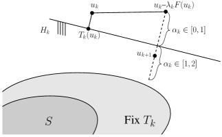
Figure 1: One step of the outer approximation method (1.3)–(1.5).

The outer approximation method has it roots in the work of Fukushima [22], where $S=\{x\in\mathbb{R}^{d}\colon s(x)\leq 0\}$ is a sublevel set of some convex function $s\colon\mathbb{R}^{d}\to\mathbb{R}$ and $H_{k}:=\{x\in\mathbb{R}^{d}\colon s(x_{k})+\langle g_{k},x-x_{k}\rangle\leq 0\}$ is a sublevel set of the linearization of $s$ at the point $x_{k}$ with $g_{k}\in\partial s(x_{k})$. In this case $T_{k}:=P_{s}$ is the subgradient projection related to $s$. Other instances of this method can be found, for example, in [14, 19, 23, 27, 26].

As it was already observed in [24], by a proper choice of the starting point, the outer approximation method can also be considered a particular case of the hybrid steepest descent method

$$u_{0}\in\mathcal{H};\qquad u_{k+1}:=R_{k}(u_{k})-\lambda_{k}F(R_{k}(u_{k})),\qquad k=0,1,2,\ldots,$$ (1.6)

in which case $R_{k}\colon\mathcal{H}_{1}\to\mathcal{H}_{1}$ may be general $\rho_{k}$-strongly quasi-nonexpansive operators with $S\subseteq\operatorname*{Fix}R_{k}$ and $\inf_{k}\rho_{k}>0$. Other works related to the above method can be found, for example, in [1, 2, 9, 13, 16, 17, 21, 37, 38, 39] and even more general methods can be found in [10].

We now recall one of the main results of [24, Theorem 3.1] which concerns method (1.3). Note that exactly the same result holds for method (1.6); see [40, Theorem 3.16] or [24, Theorem 2.17].

Theorem 1.1.

If $\lim_{k\to\infty}\lambda_{k}=0$, then the sequence $\{u_{k}\}_{k=0}^{\infty}$ is bounded. Moreover, if there is an integer $s\geq 1$ such that for each subsequence $\{n_{k}\}_{k=0}^{\infty}\subseteq\{k\}_{k=0}^{\infty}$, we have

$$\lim_{k\to\infty}\sum_{l=0}^{s-1}\|T_{n_{k}-l}(u_{n_{k}-l})-u_{n_{k}-l}\|=0\quad\Longrightarrow\quad\lim_{k\to\infty}d(u_{n_{k}},S)=0,$$ (1.7)

then $\lim_{k\rightarrow\infty}d(u_{k},S)=0$. If, in addition, $\sum_{k=0}^{\infty}\lambda_{k}=\infty$, then the sequence $\{u_{k}\}_{k=0}^{\infty}$ converges in norm to the unique solution of VI($F$, $S$).

In this paper we investigate the outer approximation method while assuming that $S$ is the solution set of the (multiple-set) split convex feasibility problem, that is,

$$S:=\left\{z\in\mathcal{H}_{1}\mid z\in C:=\bigcap_{i\in I}C_{i}\quad\text{and}\quad Az\in Q:=\bigcap_{j\in J}Q_{j}\right\}=C\cap A^{-1}(Q),$$ (1.8)

where $A\colon\mathcal{H}_{1}\rightarrow\mathcal{H}_{2}$ is a bounded linear operator and where each $C_{i}\subseteq\mathcal{H}_{1}$ and $Q_{j}\subseteq\mathcal{H}_{2}$ are closed and convex, $i\in I:=\{1,\ldots,m\}$, $j\in J:=\{1,\ldots,n\}$.

We propose a very general framework of constructing half-spaces $H_{k}$ that takes into account both the split and the multiple-set structure of the constraint set $S$. To this end, similarly to Theorem 1.1, we assume that we are given two sequences of strongly quasi-nonexpansive operators $\{\mathcal{U}_{k}\colon\mathcal{H}_{1}\to\mathcal{H}_{1}\}_{k=0}^{\infty}$ and $\{\mathcal{V}_{k}\colon\mathcal{H}_{2}\to\mathcal{H}_{2}\}_{k=0}^{\infty}$ for which $C\subseteq\operatorname*{Fix}\mathcal{U}_{k}$ and $Q\subseteq\operatorname*{Fix}\mathcal{V}_{k}$.

Examples of such operators can be obtained by simply using the metric projections $P_{C_{i}}$ and $P_{Q_{j}}$ organized in cyclic, simultaneous or block iterative ways. A similar strategy could be applied to sublevel sets, where $C_{i}:=\{x\in\mathcal{H}_{1}\colon c_{i}(x)\leq 0\}$ and $Q_{j}:=\{y\in\mathcal{H}_{2}\colon q_{j}(y)\leq 0\}$ for weakly lower semicontinuous and convex functions $c_{i}\colon\mathcal{H}_{1}\to\mathbb{R}$ and $q_{j}\colon\mathcal{H}_{2}\to\mathbb{R}$ or, in the general fixed point setting, where $C_{i}:=\operatorname*{Fix}U_{i}$ and $Q_{j}:=\operatorname*{Fix}V_{j}$ with cutters $U_{i}$ and $V_{j}$. In the former case the metric projections should be replaced by subgradient projections $P_{c_{i}}$ and $P_{q_{j}}$ whereas in the latter case one should simply use $U_{i}$ and $V_{j}$. For more details see Example 3.5 below.

The main difficulty in finding an explicit formulation for the half-spaces $H_{k}$, as they are defined in (1.5), lies in the sets $A^{-1}(Q)$ and $A^{-1}(Q_{j})$ the projections onto which are, in general, computationally expensive. We overcome this difficulty by using the so called (extrapolated) Landweber transform (see Definitions 2.9 and 2.10). Roughly speaking, the Landweber transform can be considered a formalization of several techniques used for solving split feasibility problems many of which originate in the Landweber method [28]. In particular, it can be informally found in the well-known $CQ$-method introduced by Byrne [6, 7] and further studied in [11, 13, 20, 31, 33, 35, 36]. The simultaneous counterparts of the $CQ$-method can be found in [11, 18, 20, 30, 34]. Such a transform, when applied to an operator on $\mathcal{H}_{2}$, say $\mathcal{V}_{k}$, defines a new operator on $\mathcal{H}_{1}$, which we denote by $\mathcal{L}\{\mathcal{V}_{k}\}$. As it was summarized in [15], the Landweber transform preserves many of the relevant properties of its input operator. In addition, under some assumptions, which are satisfied in our case, we have $\operatorname*{Fix}\mathcal{L}\{\mathcal{V}_{k}\}=A^{-1}(\operatorname*{Fix}\mathcal{V}_{k})$, which makes it a very suitable tool for handling split problems. The extrapolated Landweber transform has it roots in [29] and can also be found in [12].

Our main contribution in the present paper is to propose three approaches to define the half-spaces $H_{k}$, which under certain conditions, guarantee the norm convergence of the generated iterates to the unique solution of the variational inequality (1.1) over the subset S defined by (1.8). The first one is based on the product of the operators $\mathcal{U}_{k}$ and $\mathcal{L}\{\mathcal{V}_{k}\}$, which for $\mathcal{U}_{k}=P_{C}$ and $\mathcal{V}_{k}=P_{Q}$ resembles the $CQ$-method. The second one is based on averaging between $\mathcal{U}_{k}$ and $\mathcal{L}\{\mathcal{V}_{k}\}$, which corresponds to the simultaneous $CQ$-method, whereas the third variant relies on the alternating use of $\mathcal{U}_{k}$ and $\mathcal{L}\{\mathcal{V}_{k}\}$; see Theorem 3.1 for more details. In our convergence analysis, we impose two conditions on the sequences $\{\mathcal{U}_{k}\}_{k=0}^{\infty}$ and $\{\mathcal{V}_{k}\}_{k=0}^{\infty}$ which, when combined with an additional bounded regularity of two families of sets, guarantee (1.7). In particular, when $S=C$ is the solution set of the convex feasibility problem, then we obtain another convergence result along the lines of Theorem 1.1; see Theorem 3.7. Furthermore, we provide several examples of defining $\mathcal{U}_{k}$ and $\mathcal{V}_{k}$ depending on the representation of the constraint sets $C_{i}$ and $Q_{j}$; see Example 3.5.

Our paper is organized as follows. In section 2 we provide necessary tools to be used in our convergence analysis. In particular, we recall the closed range theorem, some basic properties of quasi-nonexpansive operators, regular operators and the Landweber transform. In section 3 we present our main result (Theorem 3.1) together with some examples.

2 Preliminaries

Let $\mathcal{H},\ \mathcal{H}_{1}$ and $\mathcal{H}_{2}$ be real Hilbert spaces. We denote by $\mathcal{N}(A)$, $\mathcal{R}(A)$ and $\|A\|$ the null space, the range and the norm of a bounded linear operator $A\colon\mathcal{H}_{1}\rightarrow\mathcal{H}_{2}$, respectively. It is not difficult to see that

$$\|A\|:=\sup\{\|Ax\|\colon x\in\mathcal{N}(A)^{\perp}\text{ and }\|x\|=1\}.$$ (2.1)

Analogously, we define

$$|A|:=\inf\{\|Ax\|\colon x\in\mathcal{N}(A)^{\perp}\text{ and }\|x\|=1\}.$$ (2.2)

Theorem 2.1 (Closed Range Theorem).

Let $A\colon\mathcal{H}_{1}\rightarrow\mathcal{H}_{2}$ be a nonzero bounded linear operator. Then the following statements are equivalent:

1. $\mathcal{R}(A)$ is closed;

2. $\mathcal{R}(A^{*})$ is closed;

3. $\mathcal{R}(AA^{*})$ is closed;

4. $\mathcal{R}(A^{*}A)$ is closed;

5. $\mathcal{R}(A)=(\mathcal{N}(A^{*})^{\perp}$;

6. $\mathcal{R}(A^{*})=\mathcal{N}(A)^{\perp}$;

7. $\mathcal{R}(AA^{*})=\mathcal{N}(AA^{*})^{\perp}$;

8. $\mathcal{R}(A^{*}A)=\mathcal{N}(A^{*}A)^{\perp}$;

9. $|A|>0$;

10. $|A^{*}|>0$;

11. $|AA^{*}|>0$;

12. $|A^{*}A|>0$.

Moreover, we have

$$|A|=|A^{*}|=\sqrt{|A^{*}A|}=\sqrt{|AA^{*}|}.$$ (2.3)

• See [15, Lemma 3.2]. $\blacksquare$

Remark 2.2.

Recall that the norm of $A$ satisfies $\|A\|=\|A^{*}\|=\sqrt{\|A^{*}A\|}=\sqrt{\|AA^{*}\|}$. Moreover, by the definition of $|A|$ and $\|A\|$, for all $x\in\mathcal{N}(A)^{\perp}$, we have

$$|A|\cdot\|x\|\leq\|Ax\|\leq\|A\|\cdot\|x\|.$$ (2.4)

2.1 Quasi-Nonexpansive Operators

For a given $U\colon\mathcal{H}\rightarrow\mathcal{H}$ and $\alpha\in(0,\infty)$, the operator $U_{\alpha}:=\operatorname*{Id}+\alpha(U-\operatorname*{Id})$ is called an $\alpha$-relaxation of $U$, where by $\operatorname*{Id}$ we denote the identity operator. We call $\alpha$ a relaxation parameter. It is easy to see that for every such $\alpha$, $\operatorname*{Fix}U=\operatorname*{Fix}U_{\alpha}$, where $\operatorname*{Fix}U:=\{z\in\mathcal{H}\mid U(z)=z\}$ is the fixed point set of $U$.

Definition 2.3.

Let $U\colon\mathcal{H}\rightarrow\mathcal{H}$ be an operator with a fixed point, that is, $\operatorname*{Fix}U\neq\emptyset$. We say that $U$ is

1. quasi-nonexpansive (QNE) if for all $x\in\mathcal{H}$ and all $z\in\operatorname*{Fix}U$,

   $$\|U(x)-z\|\leq\|x-z\|;$$ (2.5)

2. $\rho$-strongly quasi-nonexpansive ($\rho$-SQNE), where $\rho\geq 0$, if for all $x\in\mathcal{H}$ and all $z\in\operatorname*{Fix}U$,

   $$\|U(x)-z\|^{2}\leq\|x-z\|^{2}-\rho\|U(x)-x\|^{2};$$ (2.6)

3. a cutter if for all $x\in\mathcal{H}$ and all $z\in\operatorname*{Fix}U$,

   $$\langle z-U(x),x-U(x)\rangle\leq 0.$$ (2.7)

For a historical and mathematical overview of the above-mentioned operators we refer the reader to [8].

Theorem 2.4.

Let $U\colon\mathcal{H}\to\mathcal{H}$ be an operator with $\operatorname*{Fix}U\neq\emptyset$ and let $\rho\geq 0$. Then the operator $U$ is $\rho$-SQNE if and only if $\operatorname*{Id}+\frac{1+\rho}{2}(U-\operatorname*{Id})$ is a cutter.

• See, for example, [8, Corollary 2.1.43]. $\blacksquare$

Theorem 2.5.

Let $U_{i}\colon\mathcal{H}\to\mathcal{H}$ be $\rho_{i}$-SQNE, where $\rho_{i}>0$, $i=1,\ldots,m$. If $\bigcap_{i=1}^{m}\operatorname*{Fix}U_{i}\neq\emptyset$, then the operator $U:=\sum_{i=1}^{m}\omega_{i}U_{i}$, where $\omega_{i}>0$, $\sum_{i=1}^{m}\omega_{i}=1$, is $\rho$-SQNE with

$$\rho:=\left[\left(\sum_{i=1}^{m}\frac{\omega_{i}}{\rho_{i}+1}\right)^{-1}-1\right]\geq\min\rho_{i}>0$$ (2.8)

and $\operatorname*{Fix}U=\bigcap_{i=1}^{m}\operatorname*{Fix}U_{i}$. Moreover, for all $x\in\mathcal{H}$, we have

$$2d(x,\operatorname*{Fix}U)\cdot\left\|U(x)-x\right\|\geq\sum_{i=1}^{m}\omega_{i}\rho_{i}\|U_{i}(x)-x\|^{2}.$$ (2.9)

• See [8, Theorem 2.1.50] and [17, Proposition 4.5]. $\blacksquare$

Theorem 2.6.

Let $U_{i}\colon\mathcal{H}\to\mathcal{H}$ be $\rho_{i}$-SQNE. If $\bigcap_{i=1}^{m}\operatorname*{Fix}U_{i}\neq\emptyset$, then the operator $U:=U_{m}\ldots U_{1}$ is $\rho$-SQNE with

$$\rho:=\left(\sum_{i=1}^{m}\frac{1}{\rho_{i}}\right)^{-1}\geq\frac{\min\rho_{i}}{m}>0$$ (2.10)

and $\operatorname*{Fix}U=\bigcap_{i=1}^{m}\operatorname*{Fix}U_{i}$. Moreover, for all $x\in\mathcal{H}$, we have

$$2d(x,\operatorname*{Fix}U)\cdot\|U(x)-x\|\geq\sum_{i=1}^{m}\rho_{i}\|Q_{i}(x)-Q_{i-1}(x)\|^{2},$$ (2.11)

where $Q_{i}:=U_{i}\ldots U_{1}$ and $Q_{0}:=\operatorname*{Id}$.

• See [8, Theorems 2.1.48] and [17, Proposition 4.6]. $\blacksquare$

Example 2.7 (Subgradient Projection).

Let $f\colon\mathcal{H}\to\mathbb{R}$ be a weakly lower semicontinuous and convex function with nonempty sublevel set $S:=\{x\in\mathcal{H}\colon f(x)\leq 0\}$. For each $x\in\mathcal{H}$, let $g(x)$ be a chosen subgradient from the subdifferential set $\partial f(x):=\{g\in\mathcal{H}\colon f(y)\geq f(x)+\langle g,y-x\rangle\text{ for all }y\in\mathcal{H}\}$, which, by [5, Proposition 16.27], is nonempty. The subgradient projection operator $P_{f}\colon\mathcal{H}\to\mathcal{H}$ is defined by

$$P_{f}(x):=x-\frac{f(x)}{\|g(x)\|^{2}}g(x)$$ (2.12)

whenever $f(x)>0$ and $P_{f}(x):=x$, otherwise. One can show that $P_{f}$ is a cutter and $\operatorname*{Fix}P_{f}=S$; see, for example, [8, Corollary 4.2.6].

Example 2.8 (Proximal Operator).

Let $f\colon\mathcal{H}\to\mathbb{R}$ be a weakly lower semicontinuous and convex function. The proximal operator, defined by

$$\operatorname*{prox}\nolimits_{f}(x):=\operatorname*{argmin}_{y\in\mathcal{H}}\left(f(y)+\frac{1}{2}\|y-x\|^{2}\right),$$ (2.13)

is firmly nonexpansive and $\operatorname*{Fix}(\operatorname*{prox}_{f})=\operatorname*{Argmin}_{x\in\mathcal{H}}f(x)$; see [5, Propositions 12.28 and 12.29]. Thus if $f$ has at least one minimizer, then $\operatorname*{prox}_{f}$ is a cutter; see [8, Theorem 2.2.5.].

2.2 Landweber Transform

Let $A:\mathcal{H}_{1}\rightarrow\mathcal{H}_{2}$ be a nonzero bounded linear operator, let $V\colon\mathcal{H}_{2}\to\mathcal{H}_{2}$ be an arbitrary operator and let $\sigma\colon\mathcal{H}_{1}\to[1,\infty)$ be a given functional.

Definition 2.9.

The operator $\mathcal{L}\{V\}:\mathcal{H}_{1}\to\mathcal{H}_{1}$ defined by

$$\mathcal{L}\{V\}(x):=x+\frac{1}{\|A\|^{2}}A^{*}\big{(}V(Ax)-Ax\big{)},\quad x\in\mathcal{H}_{1},$$ (2.14)

is called the Landweber operator (corresponding to $V$). The operation $V\mapsto\mathcal{L}\{V\}$ is called the Landweber transform.

Definition 2.10.

The operator $\mathcal{L}_{\sigma}\{V\}:\mathcal{H}_{1}\to\mathcal{H}_{1}$ defined by

$$\mathcal{L}_{\sigma}\{V\}(x):=x+\frac{\sigma(x)}{\|A\|^{2}}A^{*}\big{(}V(Ax)-Ax\big{)},\quad x\in\mathcal{H}_{1},$$ (2.15)

is called the extrapolated Landweber operator (corresponding to $V$ and $\sigma$). The operation $V\mapsto\mathcal{L}_{\sigma}\{V\}$ is called the extrapolated Landweber transform.

Remark 2.11.

In this paper we only consider those extrapolation functionals $\sigma$ which are bounded from above by $\tau\colon\mathcal{H}_{1}\to[1,\infty)$ defined by

$$\tau(x):=\left(\frac{\|A\|\cdot\|V(Ax)-Ax\|}{\|A^{*}(V(Ax)-Ax)\|}\right)^{2}$$ (2.16)

whenever $V(Ax)\neq Ax$ and $\tau(x):=1$ otherwise. Note that $\mathcal{L}_{\tau}\{V\}(x)$ does not depend on $\|A\|$.

Theorem 2.12.

If $V$ is a $\rho$-SQNE operator, where $\rho\geq 0$, and $\mathcal{R}(A)\cap\operatorname*{Fix}V\neq\emptyset$, then for every extrapolation functional $\sigma$, where $1\leq\sigma\leq\tau$, the operator $\mathcal{L}_{\sigma}\{V\}$ is $\rho$-SQNE with $\operatorname*{Fix}\mathcal{L}_{\sigma}\{V\}=A^{-1}(\operatorname*{Fix}V)$. Moreover, for all $x\in\mathcal{H}_{1}$, we have

$$2d(x,\operatorname*{Fix}\mathcal{L}_{\sigma}\{V\})\cdot\|\mathcal{L}_{\sigma}\{V\}(x)-x\|\geq\frac{\rho+1}{\|A\|^{2}}\|V(Ax)-Ax\|^{2}$$ (2.17)

and if, in addition, the set $\mathcal{R}(A)$ is closed, then

$$\frac{1}{\|A\|}d(Ax,\mathcal{R}(A)\cap\operatorname*{Fix}V)\leq d(x,\operatorname*{Fix}\mathcal{L}_{\sigma}\{V\})\leq\frac{1}{|A|}d(Ax,\mathcal{R}(A)\cap\operatorname*{Fix}V).$$ (2.18)

• See, for example, [13, Theorem 4.1] for the first two statements. Inequality (2.17) follows from [15, Lemmata 4.4 and 4.6] in the case $\sigma=1$. In the general case, where we allow $\sigma(x)\geq 1$, we use the estimate $\|\mathcal{L}_{\sigma}\{V\}(x)-x\|=\sigma(x)\|\mathcal{L}\{V\}(x)-x\|\geq\|\mathcal{L}\{V\}(x)-x\|$ and the equality $\operatorname*{Fix}\mathcal{L}_{\sigma}\{V\}=\mathcal{L}\{V\}$. Inequality (2.18) follows from [15, Lemma 4.4]. $\blacksquare$

For each pair $x,x^{\prime}\in\mathcal{H}_{1}$, let $\mathcal{H}_{1}(x,x^{\prime}):=\{z\in\mathcal{H}_{1}\colon\langle x-x^{\prime},z-x^{\prime}\rangle\leq 0\}.$ Similarly, for every pair $y,y^{\prime}\in\mathcal{H}_{2}$, define $\mathcal{H}_{2}(y,y^{\prime}):=\{w\in\mathcal{H}_{2}\colon\langle y-y^{\prime},w-y^{\prime}\rangle\leq 0\}.$ We have the following lemma.

Lemma 2.13.

Assume that $V$ is a cutter and $\mathcal{R}(A)\cap\operatorname*{Fix}V\neq\emptyset$. Then for any $u\in\mathcal{H}_{1}$, the set $H:=\mathcal{H}_{1}(u,\mathcal{L}_{\tau}\{V\}(u))$ satisfies

$$H=\{z\in\mathcal{H}_{1}\colon\langle Au-V(Au),Az-V(Au)\rangle\leq 0\}=A^{-1}\big{(}\mathcal{H}_{2}(Au,V(Au))\big{)}.$$ (2.19)

Moreover,

$$P_{H}(x)=x-\frac{(\langle Au-V(Au),Ax-V(Au)\rangle)_{+}}{\|A^{*}(Au-V(Au))\|^{2}}A^{*}(Au-V(Au))$$ (2.20)

whenever $Au\neq V(Au)$ and $P_{H}(x)=x$, otherwise.

• Assume that $Au=V(Au)$ for some $u\in\mathcal{H}_{1}$. It is easy to see that in this case all the sets in (2.19) are equal to $\mathcal{H}_{1}$ and hence $P_{H}(x)=x$. Assume now that $Au\neq V(Au)$. This implies, by Theorem 2.12, that $u\neq\mathcal{L}_{\tau}\{V\}(u)$. A direct calculation shows that

  $$H =\{z\in\mathcal{H}_{1}\colon\langle u-\mathcal{L}_{\tau}\{V\}(u),z-\mathcal{L}_{\tau}\{V\}(u)\rangle\leq 0\}$$

  $$=\left\{z\in\mathcal{H}_{1}\colon\left\langle-\frac{\tau(u)}{\|A\|^{2}}A^{*}(V(Au)-Au),z-u-\frac{\tau(u)}{\|A\|^{2}}A^{*}(V(Au)-Au)\right\rangle\leq 0\right\}$$

  $$=\{z\in\mathcal{H}_{1}\colon-\langle A^{*}(V(Au)-Au),z-u\rangle+\|V(Au)-Au\|^{2}\leq 0\}$$

  $$=\{z\in\mathcal{H}_{1}\colon\langle Au-V(Au),Az-Au\rangle+\|Au-V(Au)\|^{2}\leq 0\}$$

  $$=\{z\in\mathcal{H}_{1}\colon\langle Au-V(Au),Az-V(Au)\rangle\leq 0\}$$

  $$=\{z\in\mathcal{H}_{1}\colon Az\in\mathcal{H}_{2}(Au,V(Au))\}$$

  $$=A^{-1}\big{(}\mathcal{H}_{2}(Au,V(Au))\big{)}.$$ (2.21)

  In order to show formula (2.20) it suffices to represent the half-space $H$ as $\{z\in\mathcal{H}_{1}\colon\langle a,z\rangle\leq\beta\}$ with nonzero $a\in\mathcal{H}_{1}$ and $\beta\in\mathbb{R}$ for which $P_{H}(x)=x-\frac{(\langle a,x\rangle-\beta)_{+}}{\|a\|^{2}}a$; see [8, Chapter 4]. $\blacksquare$

Lemma 2.14.

Let $P_{q}$ be a subgradient projection for a weakly lower semicontinuous function $q\colon\mathcal{H}_{2}\to\mathbb{R}$ with the corresponding subgradients $h(y)\in\partial q(y)$, $y\in\mathcal{H}_{2}$, and assume that $q(Az)\leq 0$ for some $z\in\mathcal{H}_{1}$. Then for any $u\in\mathcal{H}_{1}$, the set $H:=\mathcal{H}_{1}(u,\mathcal{L}_{\tau}\{P_{q}\}(u))$ satisfies

$$H=\{z\in\mathcal{H}_{1}\colon q(Au)+\langle A^{*}h(Au),z-u\rangle\leq 0\}$$ (2.22)

whenever $q(Au)>0$ and $H=\mathcal{H}_{1}$, otherwise. Consequently,

$$P_{H}(x)=x-\frac{(q(Au)+\langle A^{*}h(Au),x-u\rangle)_{+}}{\|A^{*}h(Au)\|^{2}}A^{*}h(Au)$$ (2.23)

whenever $q(Au)>0$ and $P_{H}(x)=x$, otherwise.

• Fix a point $u\in\mathcal{H}_{1}$. Assume first that $q(Au)\leq 0$. Since $\operatorname*{Fix}P_{q}=\{y\in\mathcal{H}_{2}\colon q(y)\leq 0\}$ (see Example 2.7), we see that $Au=P_{q}(Au)$. Consequently, $u=\mathcal{L}_{\tau}\{V\}(u)$ and thus $H=\mathcal{H}_{1}$. Now assume that $q(Au)>0$ in which case $Au\neq P_{q}(Au)$. Let $h(Au)\in\partial q(Au)$. Then, by (2.19) applied to $V=P_{q}$, we obtain

  $$H =\{z\in\mathcal{H}_{1}\colon\langle Au-P_{q}(Au),Az-P_{q}(Au)\rangle\leq 0\}$$

  $$=\left\{z\in\mathcal{H}_{1}\colon\left\langle\frac{q(Au)}{\|h(Au)\|^{2}}h,(Az-Au)+\frac{q(Au)}{\|h(Au)\|^{2}}h(Au)\right\rangle\leq 0\right\}$$

  $$=\{z\in\mathcal{H}_{1}\colon\langle A^{*}h(Au),z-u\rangle+q(Au)\leq 0\}.$$ (2.24)

  Equation (2.23) follows by the same argument as in the proof of Lemma 2.13. $\blacksquare$

Remark 2.15.

In view of [5, Theorem 16.47], we get $A^{*}\partial q(Au)=\partial(q\circ A)(u)$. Consequently, the half-space $H$ defined in (2.22) becomes a sublevel set of the functional $q\circ A$ linearized at $u$.

2.3 Regular sets

Let $C_{i}\subseteq\mathcal{H}$, $i\in I$, be closed and convex sets with a nonempty intersection $C$. Following Bauschke [3, Definition 2.1], we propose the following definition.

Definition 2.16.

We say that the family $\mathcal{C}:=\{C_{i}\mid i\in I\}$ is boundedly regular if for any bounded sequence $\{x_{k}\}_{k=0}^{\infty}\subseteq\mathcal{H}$, the following implication holds:

$$\lim_{k\rightarrow\infty}\max_{i\in I}d(x_{k},C_{i})=0\quad\Longrightarrow\quad\lim_{k\rightarrow\infty}d(x_{k},C)=0.$$ (2.25)

Example 2.17.

If at least one of the following conditions is satisfied: (i) $\dim\mathcal{H}<\infty$, (ii) $\operatorname*{int}\bigcap_{i\in I}C_{i}\neq\emptyset$ or (iii) each $C_{i}$ is a half-space, then the family $\mathcal{C}:=\{C_{i}\mid i\in I\}$ is boundedly regular; see [4].

2.4 Regular Operators

Definition 2.18.

We say that a quasi-nonexpansive operator $U\colon\mathcal{H}\rightarrow\mathcal{H}$ is boundedly regular if for any bounded sequence $\{x_{k}\}_{k=0}^{\infty}\subseteq\mathcal{H}$, we have

$$\lim_{k\to\infty}\|U(x_{k})-x_{k}\|=0\quad\Longrightarrow\quad\lim_{k\to\infty}d(x_{k},\operatorname*{Fix}U)=0.$$ (2.26)

Notation 2.19.

We define $\prod_{j\in J}U_{j}:=U_{j_{m}}\ldots U_{j_{1}}$ to be the product of operators $U_{i}\colon\mathcal{H}\to\mathcal{H}$, $i\in I$, over a nonempty ordered index set $J=(j_{1},\ldots,j_{m})\subseteq I$.

Theorem 2.20.

Let $U_{i}\colon\mathcal{H}\rightarrow\mathcal{H}$ be boundedly regular cutters, $i\in I=\{1,\ldots,m\}$ and assume that $\bigcap_{i\in I}\operatorname*{Fix}U_{i}\neq\emptyset$. For each $k=0,1,2,\ldots,$ let $I_{k}\subseteq I$ be a nonempty (ordered) subset, $|I_{k}|\leq m$ and let $0<\omega\leq\omega_{i,k}\leq 1$ be such that $\sum_{i\in I_{k}}\omega_{i,k}=1$. Then for every bounded sequence $\{x_{k}\}_{k=0}^{\infty}\subseteq\mathcal{H}$, we have

$$\lim_{k\to\infty}\left\|\sum_{i\in I_{k}}\omega_{i,k}U_{i}(x_{k})-x_{k}\right\|=0\quad\Longrightarrow\quad\lim_{k\to\infty}\max_{i\in I_{k}}d(x_{k},\operatorname*{Fix}U_{i})=0$$ (2.27)

and

$$\lim_{k\to\infty}\left\|\prod_{i\in I_{k}}U_{i}(x_{k})-x_{k}\right\|=0\quad\Longrightarrow\quad\lim_{k\to\infty}\max_{i\in I_{k}}d(x_{k},\operatorname*{Fix}U_{i})=0.$$ (2.28)

• See, either [40, Lemma 4.11] or [32, Lemma 3.5]. $\blacksquare$

3 Main Result

Theorem 3.1.

Let $F\colon\mathcal{H}_{1}\rightarrow\mathcal{H}_{1}$ be $L$-Lipschitz continuous and $\alpha$-strongly monotone, and let $S\subseteq\mathcal{H}_{1}$ be the nonempty solution set of the split convex feasibility problem, that is,

$$S:=\left\{z\in\mathcal{H}_{1}\mid z\in C:=\bigcap_{i\in I}C_{i}\quad\text{and}\quad Az\in Q:=\bigcap_{i\in J}Q_{j}\right\},$$ (3.1)

where each $C_{i}\subseteq\mathcal{H}_{1}$, $Q_{j}\subseteq\mathcal{H}_{2}$ are closed and convex, $i\in I:=\{1,\ldots,m\}$, $j\in J:=\{1,\ldots,n\}$ and where $A\colon\mathcal{H}_{1}\rightarrow\mathcal{H}_{2}$ is a bounded linear operator. Moreover, for each $k=0,1,2,\ldots$, let $\mathcal{U}_{k}\colon\mathcal{H}_{1}\to\mathcal{H}_{1}$ be $\beta_{k}$-SQNE with $C\subseteq\operatorname*{Fix}\mathcal{U}_{k}$ and $\beta:=\inf\beta_{k}>0$, and let $\mathcal{V}_{k}\colon\mathcal{H}_{2}\rightarrow\mathcal{H}_{2}$ be $\gamma_{k}$-SQNE with $Q\subseteq\operatorname*{Fix}\mathcal{V}_{k}$ and $\gamma:=\inf_{k}\gamma_{k}>0$. Furthermore, for each $k=0,1,2,\ldots$, let $\sigma_{k}\colon\mathcal{H}_{1}\to[1,\infty)$ be an extrapolation functional bounded from above by $\tau_{k}\colon\mathcal{H}_{1}\to[1,\infty)$ defined by

$$\tau_{k}(x):=\left(\frac{\|A\|\cdot\|\mathcal{V}_{k}(Ax)-Ax\|}{\|A^{*}(\mathcal{V}_{k}(Ax)-Ax)\|}\right)^{2}$$ (3.2)

whenever $\mathcal{V}_{k}(Ax)\neq Ax$ and $\tau_{k}(x):=1$, otherwise. Let the sequence $\{u_{k}\}_{k=0}^{\infty}$ be defined by the outer approximation method (1.3)–(1.5) combined with one of the following algorithmic operators $T_{k}$:

1. product operators, where

   $$T_{k}(x):=x+\frac{1+\rho_{k}}{2}\Big{(}\mathcal{U}_{k}(\mathcal{L}_{\sigma_{k}}\{\mathcal{V}_{k}\}(x))-x\Big{)},$$ (3.3)

   $$0\leq\rho_{k}\leq\left(\frac{1}{\beta_{k}}+\frac{1}{\gamma_{k}}\right)^{-1};$$ (3.4)

2. simultaneous operators, where $0<\eta\leq\eta_{k}\leq 1-\eta$,

   $$T_{k}(x):=x+\frac{1+\rho_{k}}{2}\big{(}\eta_{k}\mathcal{U}_{k}(x)+(1-\eta_{k})\mathcal{L}_{\sigma_{k}}\{\mathcal{V}_{k}\}(x)-x\big{)},$$ (3.5)

   $$0\leq\rho_{k}\leq\left(\frac{\eta_{k}}{\beta_{k}+1}+\frac{1-\eta_{k}}{\gamma_{k}+1}\right)^{-1}-1;$$ (3.6)

3. alternating operators, where

   $$T_{2k}(x):=x+\frac{1+\beta_{k}}{2}\big{(}\mathcal{U}_{k}(x)-x\big{)}\qquad\text{and}\qquad T_{2k+1}(x):=x+\frac{1+\gamma_{k}}{2}\big{(}\mathcal{L}_{\sigma_{k}}\{\mathcal{V}_{k}\}(x)-x\big{)}.$$ (3.7)

Assume that for all bounded sequences $\{x_{k}\}_{k=0}^{\infty}\subseteq\mathcal{H}_{1}$ and $\{y_{k}\}_{k=0}^{\infty}\subseteq\mathcal{H}_{2}$, we have

$$\lim_{k\to\infty}\|\mathcal{U}_{k}(x_{k})-x_{k}\|=0\quad\Longrightarrow\quad\lim_{k\to\infty}\max_{i\in I_{k}}d(x_{k},C_{i})=0,$$ (3.8)

and

$$\lim_{k\to\infty}\|\mathcal{V}_{k}(y_{k})-y_{k}\|=0\quad\Longrightarrow\quad\lim_{k\to\infty}\max_{j\in J_{k}}d(y_{k},Q_{j})=0,$$ (3.9)

where $I_{k}\subseteq I$ and $J_{k}\subseteq J$ are not empty and $|I_{k}|\leq m$, $|J_{k}|\leq n$. If $\{I_{k}\}_{k=0}^{\infty}$ and $\{J_{k}\}_{k=0}^{\infty}$ are $s$-intermittent for some $s\geq 1$ (that is, $I=I_{k}\cup\ldots\cup I_{k+s-1}$, $J=J_{k}\cup\ldots\cup J_{k+s-1}$ for all $k\geq 0$), $\mathcal{R}(A)$ is closed, $\{A^{-1}(Q),C_{1},\ldots,C_{m}\}$ and $\{\mathcal{R}(A),Q_{1},\ldots,Q_{n}\}$ are boundedly regular, and $\lim_{k\to\infty}\lambda_{k}=0$, then $\lim_{k\to\infty}d(u_{k},S)=0$. If, in addition, $\sum_{k=0}^{\infty}\lambda_{k}=\infty$, then the sequence $\{u_{k}\}_{k=0}^{\infty}$ converges in norm to the unique solution of VI($F$, $S$).

• Observe that the operators $T_{k}$ defined either in (i), (ii) or (iii) are cutters such that $S\subseteq\operatorname*{Fix}T_{k}$. This follows from Theorems 2.4, 2.5, 2.6 and 2.12. Therefore it is reasonable to consider the outer approximation method paired with the $T_{k}$’s.

  In order to complete the proof, in view of Theorem 1.1, it suffices to show that for any subsequence $\{n_{k}\}_{k=0}^{\infty}\subseteq\{k\}_{k=0}^{\infty}$, we have

  $$\lim_{k\to\infty}\sum_{l=0}^{2s-1}\|T_{n_{k}-l}(u_{n_{k}-l})-u_{n_{k}-l}\|=0\quad\Longrightarrow\quad\lim_{k\to\infty}d(u_{n_{k}},S)=0.$$ (3.10)

  To this end, assume that

  $$\lim_{k\to\infty}\sum_{l=0}^{2s-1}\|T_{n_{k}-l}(u_{n_{k}-l})-u_{n_{k}-l}\|=0$$ (3.11)

  for some $\{n_{k}\}_{k=0}^{\infty}\subseteq\{k\}_{k=0}^{\infty}$. We divide the rest of the proof into several steps.

  Step 1. By Theorem 1.1, the sequence $\{u_{k}\}_{k=0}^{\infty}$ is bounded and hence $d(u_{k},S)\leq R$ for some $R>0$. Moreover, by [24, Lemma 3.2], for any subsequence $\{m_{k}\}_{k=0}^{\infty}\subseteq\{k\}_{k=0}^{\infty}$, we have

  $$\lim_{k\to\infty}(T_{m_{k}}(u_{m_{k}})-u_{m_{k}})=0\quad\Longleftrightarrow\quad\lim_{k\to\infty}(u_{m_{k}+1}-u_{m_{k}})=0.$$ (3.12)

  Consequently, by setting $m_{k}:=n_{k}-l$ and by (3.11), for each $l=1,2,\ldots,2s-1$, we obtain

  $$\lim_{k\to\infty}\|u_{n_{k}}-u_{n_{k}-l}\|=0.$$ (3.13)

Step 2. Observe that property (3.8), which is solely related to the sequence of operators paired with the sequence of index sets, is hereditary with respect to any of their subsequences. To be more precise, for all bounded sequences $\{x_{k}\}_{k=0}^{\infty}\subseteq\mathcal{H}_{1}$ and for any subsequence $\{m_{k}\}_{k=0}^{\infty}\subseteq\{k\}_{k=0}^{\infty}$, we have

$$\lim_{k\to\infty}\|\mathcal{U}_{m_{k}}(x_{k})-x_{k}\|=0\quad\Longrightarrow\quad\lim_{k\to\infty}\max_{i\in I_{m_{k}}}d(x_{k},C_{i})=0.$$ (3.14)

Indeed, take any $z\in S$ and define $x_{m}^{\prime}:=x_{m_{k}}$ whenever $m=m_{k}$ and otherwise set $x_{m}^{\prime}:=z$. It is not difficult to see that the augmented sequence $\{x_{m}^{\prime}\}_{n=0}^{\infty}$ is bounded and satisfies (3.8) which in turn implies (3.14).

By applying a similar argument to property (3.9), we obtain that for all bounded sequences $\{y_{k}\}_{k=0}^{\infty}\subseteq\mathcal{H}_{2}$ and for any subsequence $\{m_{k}\}_{k=0}^{\infty}\subseteq\{k\}_{k=0}^{\infty}$,

$$\lim_{k\to\infty}\|\mathcal{V}_{m_{k}}(y_{k})-y_{k}\|=0\quad\Longrightarrow\quad\lim_{k\to\infty}\max_{j\in J_{m_{k}}}d(y_{k},Q_{j})=0.$$ (3.15)

Step 3. We show that in all three cases (i)–(iii), we have

$$\lim_{k\to\infty}\max_{i\in I}d(u_{n_{k}},C_{i})=0\qquad\text{and}\qquad\lim_{k\to\infty}\max_{j\in J}d(Au_{n_{k}},Q_{j})=0.$$ (3.16)

To this end, let $i_{k}:=\operatorname*{argmax}_{i\in I}d(u_{n_{k}},C_{i})$ and let $j_{k}:=\operatorname*{argmax}_{j\in J}d(Au_{n_{k}},Q_{j})$.

Case (i). By Theorems 2.6 and 2.12, for each $l=0,1,2,\ldots,2s-1$, we have

$$\|T_{n_{k}-l}(u_{n_{k}-l})-u_{n_{k}-l}\| \geq\frac{1}{2}\|\mathcal{U}_{n_{k}-l}(\mathcal{L}_{\sigma_{n_{k}-l}}\{\mathcal{V}_{n_{k}-l}\}(u_{n_{k}-l}))-u_{n_{k}-l}\|$$

$$\geq\frac{\beta}{4R}\|\mathcal{U}_{n_{k}-l}(\mathcal{L}_{\sigma_{n_{k}-l}}\{\mathcal{V}_{n_{k}-l}\}(u_{n_{k}-l}))-\mathcal{L}_{\sigma_{n_{k}-l}}\{\mathcal{V}_{n_{k}-l}\}(u_{n_{k}-l})\|^{2}$$

$$\quad+\frac{\gamma}{4R}\|\mathcal{L}_{\sigma_{n_{k}-l}}\{\mathcal{V}_{n_{k}-l}\}(u_{n_{k}-l})-u_{n_{k}-l}\|^{2}$$

$$\geq\frac{\beta}{4R}\|\mathcal{U}_{n_{k}-l}(\mathcal{L}_{\sigma_{n_{k}-l}}\{\mathcal{V}_{n_{k}-l}\}(u_{n_{k}-l}))-\mathcal{L}_{\sigma_{n_{k}-l}}\{\mathcal{V}_{n_{k}-l}\}(u_{n_{k}-l})\|^{2}$$

$$\quad+\frac{\gamma}{16R^{3}\|A\|^{4}}\cdot\|\mathcal{V}_{n_{k}-l}(Au_{n_{k}-l})-Au_{n_{k}-l}\|^{4}.$$ (3.17)

For each $k\geq 2s-1$, let $l_{k}$ be the smallest $l\in\{0,\ldots,2s-1\}$ such that $i_{k}\in I_{n_{k}-l}$. Since the control sequence $\{I_{k}\}_{k=0}^{\infty}$ is $s$-intermittent, such an $l_{k}$ exists. By (3.11), (3) and (3.14) applied to $m_{k}:=n_{k}-l_{k}$ and $x_{k}:=\mathcal{L}_{\sigma_{n_{k}-l_{k}}}\{\mathcal{V}_{n_{k}-l_{k}}\}(u_{n_{k}-l_{k}})$, we obtain

$$\lim_{k\to\infty}\max_{i\in I_{n_{k}-l_{k}}}d(x_{k},C_{i})=0.$$ (3.18)

Moreover, by (3.11) and (3), we have

$$\lim_{k\to\infty}\|x_{k}-u_{n_{k}-l_{k}}\|=0$$ (3.19)

and consequently,

$$\max_{i\in I}d(u_{n_{k}},C_{i}) =\|P_{C_{i_{k}}}(u_{n_{k}})-u_{n_{k}}\|\leq\|P_{C_{i_{k}}}(x_{k})-u_{n_{k}}\|$$

$$\leq\|P_{C_{i_{k}}}(x_{k})-x_{k}\|+\|x_{k}-u_{n_{k}-l_{k}}\|+\|u_{n_{k}-l_{k}}-u_{n_{k}}\|$$

$$\leq\max_{i\in I_{n_{k}-l_{k}}}d(x_{k},C_{i})+\|x_{k}-u_{n_{k}-l_{k}}\|+\|u_{n_{k}-l_{k}}-u_{n_{k}}\|\to 0$$ (3.20)

as $k\to\infty$, which proves the first part of (3.16).

Similarly, for each $k\geq 2s-1$, let $r_{k}$ be the smallest $r\in\{0,\ldots,2s-1\}$ such that $j_{k}\in I_{n_{k}-r}$. By (3.11), (3) and (3.15) applied to $m_{k}:=n_{k}-r_{k}$ and $y_{k}:=Au_{n_{k}-r_{k}}$, we obtain

$$\lim_{k\to\infty}\max_{j\in J_{n_{k}-r_{k}}}d(y_{k},Q_{j})=0.$$ (3.21)

By the definition of the metric projection and by the triangle inequality, we have

$$\max_{j\in J}d(Au_{n_{k}},Q_{j}) =\|P_{Q_{j_{k}}}(Au_{n_{k}})-Au_{n_{k}}\|\leq\|P_{Q_{j_{k}}}(y_{k})-Au_{n_{k}}\|$$

$$\leq\|P_{Q_{j_{k}}}(y_{k})-y_{k}\|+\|y_{k}-Au_{n_{k}}\|$$

$$\leq\max_{j\in J_{n_{k}-r_{k}}}d(y_{k},Q_{j})+\|A\|\cdot\|u_{n_{k}}-u_{n_{k}-r_{k}}\|\to 0$$ (3.22)

as $k\to\infty$. This proves the second part of (3.16).

Case (ii). By Theorems 2.5 and 2.12, for each $l=0,1,2,\ldots,2s-1$, we have

$$\|T_{n_{k}-l}(u_{n_{k}-l})-u_{n_{k}-l}\| \geq\frac{1}{2}\|\eta_{n_{k}-l}\mathcal{U}_{n_{k}-l}(u_{n_{k}-l})+(1-\eta_{n_{k}-l})\mathcal{L}_{\sigma_{n_{k}-l}}\{\mathcal{V}_{n_{k}-l}\}(u_{n_{k}-l})\|$$

$$\geq\frac{\eta\beta}{4R}\|\mathcal{U}_{n_{k}-l}(u_{n_{k}-l})-u_{n_{k}-l})\|^{2}$$

$$\quad+\frac{\eta\gamma}{4R}\|\mathcal{L}_{\sigma_{n_{k}-l}}\{V_{n_{k}-l}\}(u_{n_{k}-l})-u_{n_{k}-l}\|^{2}$$

$$\geq\frac{\eta\beta}{4R}\|\mathcal{U}_{n_{k}-l}(u_{n_{k}-l})-u_{n_{k}-l})\|^{2}$$

$$\quad+\frac{\eta\gamma}{16R^{3}\|A\|^{4}}\cdot\frac{}{}\|\mathcal{V}_{n_{k}-l}(A(u_{n_{k}-l}))-A(u_{n_{k}-l})\|^{4}.$$ (3.23)

Similarly to Case (i), we can apply (3.14) to $m_{k}:=n_{k}-l_{k}$ and $x_{k}:=u_{n_{k}-l_{k}}$ in order to obtain (3.18) and (3). Moreover, by applying (3.15) to $m_{k}:=n_{k}-r_{k}$ and $y_{k}:=Au_{n_{k}-r_{k}}$, we obtain (3.21) and (3).

Case (iii). We split the sequence $\{n_{k}\}_{k=0}^{\infty}$ into two disjoint subsequences consisting of all odd and all even integers, respectively. To this end, consider the quotients $q_{k}:=\lfloor n_{k}/2\rfloor$, and define the sets $K_{1}:=\{k\colon n_{k}=2q_{k}+1\}$ and $K_{2}:=\{k\colon n_{k}=2q_{k}\}$. Without any loss of generality, we may assume that both $K_{1}$ and $K_{2}$ are infinite. Otherwise the argument simplifies to only one of them.

Assume for now that $k\in K_{1}$. By using the equality $n_{k}-2l-1=2(q_{k}-l)$ and by the definition of $T_{k}$, we get

$$\|T_{n_{k}-2l-1}(u_{n_{k}-2l-1})-u_{n_{k}-2l-1}\|\geq\frac{1}{2}\|\mathcal{U}_{q_{k}-l}(u_{n_{k}-2l-1})-u_{n_{k}-2l-1}\|.$$ (3.24)

Similarly, using the equality $n_{k}-2l=2(q_{k}-l)+1$, the definition of $T_{k}$ and (2.17), we obtain

$$\|T_{n_{k}-2l}(u_{n_{k}-2l})-u_{n_{k}-2l}\| \geq\frac{1}{2}\|\mathcal{L}_{\sigma_{q_{k}-l}}\{\mathcal{V}_{q_{k}-l}\}(u_{n_{k}-2l})-u_{n_{k}-2l}\|$$

$$\geq\frac{1}{4R\|A\|^{2}}\|\mathcal{V}_{q_{k}-l}(Au_{n_{k}-2l})-Au_{n_{k}-2l}\|^{2}.$$ (3.25)

Since both controls $\{I_{k}\}_{k=0}^{\infty}$ and $\{J_{k}\}_{k=0}^{\infty}$ are $s$-intermittent, for each $k\in K_{1}$, there are $l_{k},r_{k}\in\{0,\ldots,s-1\}$ such that $i_{k}\in I_{q_{k}-l_{k}}$ and $j_{k}\in J_{q_{k}-r_{k}}$. By (3.11), (3.24) and (3.14) applied to $m_{k}:=q_{k}-l_{k}$ and $x_{k}:=u_{n_{k}-2l_{k}-1}$, we obtain

$$\lim_{\begin{subarray}{c}k\to\infty\\ k\in K_{1}\end{subarray}}\ \max_{i\in I_{q_{k}-l_{k}}}d(x_{k},C_{i})=0.$$ (3.26)

Moreover (compare with (3)), we have

$$\max_{i\in I}d(u_{n_{k}},C_{i}) \leq\max_{i\in I_{q_{k}-l_{k}}}d(x_{k},C_{i})+\|u_{n_{k}}-u_{n_{k}-2l_{k}-1}\|\to 0$$ (3.27)

as $k\to\infty$, $k\in K_{1}$. On the other hand, by (3.11), (3) and (3.15) applied to $m_{k}:=q_{k}-r_{k}$ and $y_{k}:=Au_{n_{k}-2r_{k}}$, we obtain

$$\lim_{\begin{subarray}{c}k\to\infty\\ k\in K_{1}\end{subarray}}\ \max_{j\in J_{q_{k}-r_{k}}}d(y_{k},Q_{j})=0.$$ (3.28)

Moreover (compare with (3)), we have

$$\max_{j\in J}d(Au_{n_{k}},Q_{j}) \leq\max_{j\in J_{q_{k}-r_{k}}}d(y_{k},Q_{j})+\|A\|\cdot\|u_{n_{k}}-u_{n_{k}-2r_{k}}\|\to 0$$ (3.29)

as $k\to\infty$, $k\in K_{1}$. This proves (3.16) when $k\in K_{1}$.

A very similar argument can be used to show that

$$\lim_{\begin{subarray}{c}k\to\infty\\ k\in K_{2}\end{subarray}}\max_{i\in I}d(u_{n_{k}},C_{i})=0\qquad\text{and}\qquad\lim_{\begin{subarray}{c}k\to\infty\\ k\in K_{2}\end{subarray}}\max_{j\in J}d(Au_{n_{k}},Q_{j})=0.$$ (3.30)

This, when combined with (3.27) and (3.29), completes the proof of Case (iii).

Step 4. We show that in all three cases, we have $d(u_{n_{k}},S)\to 0$. Indeed, by Theorem 2.12 (with $V=P_{Q}$), we have

$$d(u_{n_{k}},A^{-1}(Q))\leq\frac{1}{|A|}d(Au_{n_{k}},\mathcal{R}(A)\cap Q).$$ (3.31)

Since $Au_{n_{k}}\in\mathcal{R}(A)$, by the second part in (3.16) and, by the assumed bounded regularity of the family $\{\mathcal{R}(A),Q_{1},\ldots,Q_{n}\}$, we obtain $d(Au_{n_{k}},\mathcal{R}(A)\cap Q)\to 0$ and thus $d(u_{n_{k}},A^{-1}(Q))\to 0$. This, when combined with the first part of (3.16) and the assumed bounded regularity of the family $\{A^{-1}(Q),C_{1},\ldots,C_{m}\}$, lead to $d(u_{n_{k}},S)\to 0$, which completes the proof. $\blacksquare$

Remark 3.2 ($CQ$-methods).

Assume that $\mathcal{U}_{k}:=P_{Q}$ and $\mathcal{V}_{k}:=P_{Q}$ for each $k=0,1,2,\ldots$. Then, within the framework of Theorem 3.1, the half-spaces $H_{k}$ are obtained by using the algorithmic operators $T_{k}$ corresponding to the (extrapolated) $CQ$-method in case (i), the simultaneous(-extrapolated) $CQ$-method in case (ii) and the alternating(-extrapolated) $CQ$-method in case (iii).

We now present several examples of sequences $\{\mathcal{U}_{k}\}_{k=0}^{\infty}$ and $\{\mathcal{V}_{k}\}_{k=0}^{\infty}$ all of which satisfy conditions (3.8) and (3.9), respectively. For this reason, assume that for each $i\in I$ and $j\in J$, we have

$$C_{i}=\operatorname*{Fix}U_{i}\qquad\text{and}\qquad Q_{j}=\operatorname*{Fix}V_{j},$$ (3.32)

where $U_{i}\colon\mathcal{H}_{1}\to\mathcal{H}_{1}$ and $V_{j}\colon\mathcal{H}_{2}\to\mathcal{H}_{2}$ are boundedly regular cutters.

Remark 3.3.

Within the above setting, one can use:

• Metric projections $U_{i}=P_{C_{i}}$ and $V_{j}=P_{Q_{j}}$.

• Subgradient projections $U_{i}=P_{c_{i}}$ and $V_{j}=P_{q_{j}}$, when $C_{i}=\{x\in\mathbb{R}^{d_{1}}\colon c_{i}(x)\leq 0\}$ and $Q_{j}=\{y\in\mathbb{R}^{d_{2}}\colon q_{j}(y)\leq 0\}$ for some convex functions $c_{i}\colon\mathbb{R}^{d_{1}}\to\mathbb{R}$ and $q_{j}\colon\mathbb{R}^{d_{2}}\to\mathbb{R}$.

• Proximal operators $U_{i}=\operatorname*{prox}_{c_{i}}$ and $V_{j}=\operatorname*{prox}_{q_{j}}$, when $C_{i}=\operatorname*{Argmin}_{x}c_{i}(x)$ and $Q_{j}=\operatorname*{Argmin}_{y}q_{j}(y)$ for $c_{i}$ and $q_{j}$ as above.

• Any firmly nonexpansive mappings $U_{i}\colon\mathbb{R}^{d_{1}}\to\mathbb{R}^{d_{1}}$ and $V_{j}\colon\mathbb{R}^{d_{2}}\to\mathbb{R}^{d_{2}}$.

Remark 3.4.

Bounded regularity of the families $\{A^{-1}(Q),C_{1},\ldots,C_{m}\}$ and $\{\mathcal{R}(A),Q_{1},\ldots,Q_{n}\}$ holds when, for example, $\mathcal{H}_{1}=\mathbb{R}^{d_{1}}$, $\mathcal{H}_{2}=\mathbb{R}^{d_{2}}$.

Example 3.5.

In view of Theorem 2.20, the operators $T_{k}$ (and thus the half-spaces $H_{k}$) presented in Theorem 3.1 (cases (i), (ii) and (iii)) can be obtained by using:

1. Sequential cutters, where

   $$\mathcal{U}_{k}:=U_{i_{k}}\qquad\text{and}\qquad\mathcal{V}_{k}:=V_{j_{k}},$$ (3.33)

   and $\{i_{k}\}_{k=0}^{\infty}\subseteq I$ and $\{j_{k}\}_{k=0}^{\infty}\subseteq J$ are two $s$-almost cyclic control sequences, that is, $I=\{i_{k},\ldots,i_{k+s-1}\}$ and $J=\{j_{k},\ldots,j_{k+s-1}\}$ for all $k\geq 0$.

2. Simultaneous cutters, where

   $$\mathcal{U}_{k}:=\sum_{i\in I_{k}}\omega_{i,k}U_{i}\qquad\text{and}\qquad\mathcal{V}_{k}:=\sum_{j\in J_{k}}\omega_{j,k}^{\prime}V_{j},$$ (3.34)

   $\{I_{k}\}_{k=0}^{\infty}\subseteq I$ and $\{J_{k}\}_{k=0}^{\infty}\subseteq J$ are $s$-intermittent control sequences, and where $\omega_{i,k},\omega_{j,k}^{\prime}\geq\omega>0$ are such that $\sum_{i\in I_{k}}\omega_{i,k}=\sum_{j\in J_{k}}\omega_{j,k}^{\prime}=1$.

3. Products of cutters, where

   $$\mathcal{U}_{k}:=\prod_{i\in I_{k}}U_{i}\qquad\text{and}\qquad\mathcal{V}_{k}:=\prod_{j\in J_{k}}V_{j},$$ (3.35)

   and $\{I_{k}\}_{k=0}^{\infty}\subseteq I$ and $\{J_{k}\}_{k=0}^{\infty}\subseteq J$ are as above.

Remark 3.6.

Observe that in the case of alternating operators (case (iii)) with the extrapolation functional $\sigma_{k}=\tau_{k}$, in view of Lemma 2.13, the half-space $H_{2k+1}$ and the associated projection $P_{H_{2k+1}}$ have equivalent forms, that is,

$$H_{2k+1}=\{z\in\mathcal{H}_{1}\colon\langle Au_{2k+1}-\mathcal{V}_{k}(Au_{2k+1}),Az-\mathcal{V}_{k}(Au_{2k+1})\rangle\leq 0\}$$ (3.36)

and

$$P_{H_{2k+1}}(x)=x-\frac{(\langle Au_{2k+1}-\mathcal{V}_{k}(Au_{2k+1}),Ax-\mathcal{V}_{k}(Au_{2k+1})\rangle)_{+}}{\|A^{*}(Au_{2k+1}-\mathcal{V}_{k}(Au_{2k+1}))\|^{2}}A^{*}(Au_{2k+1}-\mathcal{V}_{k}(Au_{2k+1}))$$ (3.37)

whenever $Au_{2k+1}\neq\mathcal{V}_{k}(Au_{2k+1})$ and otherwise $H_{2k+1}=\mathcal{H}_{1}$, in which case $P_{H_{2k+1}}(x)=x$.

By slightly adjusting the proof of Theorem 3.1, one can also obtain the following result.

Theorem 3.7.

Let $F\colon\mathcal{H}\rightarrow\mathcal{H}$ be $L$-Lipschitz continuous and $\alpha$-strongly monotone, and let $S\subseteq\mathcal{H}$ be the nonempty solution set of a convex feasibility problem, that is, $S:=\bigcap_{i\in I}C_{i}$, where $C_{i}\subseteq\mathcal{H}$ are closed and convex, $i\in I:=\{1,\ldots,m\}$. Moreover, for each $k=0,1,2,\ldots$, let $T_{k}\colon\mathcal{H}\to\mathcal{H}$ be a cutter. Let the sequence $\{u_{k}\}_{k=0}^{\infty}$ be defined by the outer approximation method (1.3)–(1.5). Assume that for all bounded sequences $\{x_{k}\}_{k=0}^{\infty}\subseteq\mathcal{H}$, we have

$$\lim_{k\to\infty}\|T_{k}(x_{k})-x_{k}\|=0\quad\Longrightarrow\quad\lim_{k\to\infty}\max_{i\in I_{k}}d(x_{k},C_{i})=0,$$ (3.38)

where $I_{k}\subseteq I$ are not empty and $|I_{k}|\leq m$. If $\{I_{k}\}_{k=0}^{\infty}$ is $s$-intermittent, $\{C_{1},\ldots,C_{m}\}$ is boundedly regular and $\lim_{k\to\infty}\lambda_{k}=0$, then $\lim_{k\to\infty}d(u_{k},S)=0$. If, in addition, $\sum_{k=0}^{\infty}\lambda_{k}=\infty$, then the sequence $\{u_{k}\}_{k=0}^{\infty}$ converges in norm to the unique solution of VI($F$, $S$).

Funding. This work was partially supported by the Israel Science Foundation (Grants 389/12 and 820/17), the Fund for the Promotion of Research at the Technion and by the Technion General Research Fund.

References

• [1] Aoyama, K., Kimura, Y.: A note on the hybrid steepest descent methods. In: Fixed point theory and its applications, pp. 73–80. Casa Cărţii de Ştiinţă, Cluj-Napoca (2013)
• [2] Aoyama, K., Kohsaka, F.: Viscosity approximation process for a sequence of quasinonexpansive mappings. Fixed Point Theory Appl. 2014:17, 11 pp. (2014)
• [3] Bauschke, H.H.: A norm convergence result on random products of relaxed projections in Hilbert space. Trans. Amer. Math. Soc. 347(4), 1365–1373 (1995)
• [4] Bauschke, H.H., Borwein, J.M.: On projection algorithms for solving convex feasibility problems. SIAM Rev. 38(3), 367–426 (1996)
• [5] Bauschke, H.H., Combettes, P.L.: Convex analysis and monotone operator theory in Hilbert spaces, second edn. CMS Books in Mathematics. Springer, Cham (2017). With a foreword by Hédy Attouch
• [6] Byrne, C.: Iterative oblique projection onto convex sets and the split feasibility problem. Inverse Problems 18(2), 441–453 (2002)
• [7] Byrne, C.: A unified treatment of some iterative algorithms in signal processing and image reconstruction. Inverse Problems 20(1), 103–120 (2004)
• [8] Cegielski, A.: Iterative methods for fixed point problems in Hilbert spaces, Lecture Notes in Mathematics, vol. 2057. Springer, Heidelberg (2012)
• [9] Cegielski, A.: Extrapolated simultaneous subgradient projection method for variational inequality over the intersection of convex subsets. J. Nonlinear Convex Anal. 15(2), 211–218 (2014)
• [10] Cegielski, A.: Application of quasi-nonexpansive operators to an iterative method for variational inequality. SIAM J. Optim. 25(4), 2165–2181 (2015)
• [11] Cegielski, A.: General method for solving the split common fixed point problem. J. Optim. Theory Appl. 165(2), 385–404 (2015)
• [12] Cegielski, A.: Landweber-type operator and its properties. In: A panorama of mathematics: pure and applied, Contemp. Math., vol. 658, pp. 139–148. Amer. Math. Soc., Providence, RI (2016)
• [13] Cegielski, A., Al-Musallam, F.: Strong convergence of a hybrid steepest descent method for the split common fixed point problem. Optimization 65(7), 1463–1476 (2016)
• [14] Cegielski, A., Gibali, A., Reich, S., Zalas, R.: An algorithm for solving the variational inequality problem over the fixed point set of a quasi-nonexpansive operator in Euclidean space. Numer. Funct. Anal. Optim. 34(10), 1067–1096 (2013)
• [15] Cegielski, A., Reich, S., Zalas, R.: Weak, strong and linear convergence of the CQ-method via the regularity of landweber operators. Optimization (2019). DOI 10.1080/02331934.2019.1598407
• [16] Cegielski, A., Zalas, R.: Methods for variational inequality problem over the intersection of fixed point sets of quasi-nonexpansive operators. Numer. Funct. Anal. Optim. 34(3), 255–283 (2013)
• [17] Cegielski, A., Zalas, R.: Properties of a class of approximately shrinking operators and their applications. Fixed Point Theory 15(2), 399–426 (2014)
• [18] Censor, Y., Elfving, T., Kopf, N., Bortfeld, T.: The multiple-sets split feasibility problem and its applications for inverse problems. Inverse Problems 21(6), 2071–2084 (2005)
• [19] Censor, Y., Gibali, A.: Projections onto super-half-spaces for monotone variational inequality problems in finite-dimensional space. J. Nonlinear Convex Anal. 9(3), 461–475 (2008)
• [20] Censor, Y., Segal, A.: The split common fixed point problem for directed operators. J. Convex Anal. 16(2), 587–600 (2009)
• [21] Deutsch, F., Yamada, I.: Minimizing certain convex functions over the intersection of the fixed point sets of nonexpansive mappings. Numer. Funct. Anal. Optim. 19(1-2), 33–56 (1998)
• [22] Fukushima, M.: A relaxed projection method for variational inequalities. Math. Programming 35(1), 58–70 (1986)
• [23] Gibali, A., Reich, S., Zalas, R.: Iterative methods for solving variational inequalities in Euclidean space. J. Fixed Point Theory Appl. 17(4), 775–811 (2015)
• [24] Gibali, A., Reich, S., Zalas, R.: Outer approximation methods for solving variational inequalities in Hilbert space. Optimization 66(3), 417–437 (2017)
• [25] Goldstein, A.A.: Convex programming in Hilbert space. Bull. Amer. Math. Soc. 70, 709–710 (1964)
• [26] He, S., Tian, H.: Selective projection methods for solving a class of variational inequalities. Numer. Algorithms 80(2), 617–634 (2019)
• [27] He, S., Yang, C.: Solving the variational inequality problem defined on intersection of finite level sets. Abstr. Appl. Anal. pp. 8, Art. ID 942,315 (2013)
• [28] Landweber, L.: An iteration formula for Fredholm integral equations of the first kind. Amer. J. Math. 73, 615–624 (1951)
• [29] López, G., Martín-Márquez, V., Wang, F., Xu, H.K.: Solving the split feasibility problem without prior knowledge of matrix norms. Inverse Problems 28(8), 085,004, pp. 18 (2012)
• [30] Masad, E., Reich, S.: A note on the multiple-set split convex feasibility problem in Hilbert space. J. Nonlinear Convex Anal. 8(3), 367–371 (2007)
• [31] Moudafi, A.: The split common fixed-point problem for demicontractive mappings. Inverse Problems 26(5), 055,007, 6 (2010)
• [32] Reich, S., Zalas, R.: A modular string averaging procedure for solving the common fixed point problem for quasi-nonexpansive mappings in Hilbert space. Numer. Algorithms 72(2), 297–323 (2016)
• [33] Wang, F., Xu, H.K.: Cyclic algorithms for split feasibility problems in Hilbert spaces. Nonlinear Anal. 74(12), 4105–4111 (2011)
• [34] Xu, H.K.: A variable Krasnosel’skiĭ-Mann algorithm and the multiple-set split feasibility problem. Inverse Problems 22(6), 2021–2034 (2006)
• [35] Xu, H.K.: Iterative methods for the split feasibility problem in infinite-dimensional Hilbert spaces. Inverse Problems 26(10), 105,018, 17 pp. (2010)
• [36] Xu, H.K.: Averaged mappings and the gradient-projection algorithm. J. Optim. Theory Appl. 150(2), 360–378 (2011)
• [37] Yamada, I.: The hybrid steepest descent method for the variational inequality problem over the intersection of fixed point sets of nonexpansive mappings. In: Inherently parallel algorithms in feasibility and optimization and their applications (Haifa, 2000), Stud. Comput. Math., vol. 8, pp. 473–504. North-Holland, Amsterdam (2001)
• [38] Yamada, I., Ogura, N.: Hybrid steepest descent method for variational inequality problem over the fixed point set of certain quasi-nonexpansive mappings. Numer. Funct. Anal. Optim. 25(7-8), 619–655 (2004)
• [39] Yu, Z.T., Chuang, C.S., Lin, L.J.: Convergence theorem for variational inequality in Hilbert spaces with applications. Numer. Funct. Anal. Optim. 39(8), 865–893 (2018)
• [40] Zalas, R.: Variational inequalities for fixed point problems of quasi-nonexpansive operators. Ph.D. thesis, University of Zielona Góra, Zielona Góra, Poland (2014). In Polish
• [41] Zeidler, E.: Nonlinear functional analysis and its applications. III, Variational methods and optimization. Springer, New York (1985)