Mass-Temperature relation in $\Lambda$CDM and modified gravity

Abstract

We derive the mass-temperature relation using an improved top-hat model and a continuous formation model which takes into account the effects of the ordered angular momentum acquired through tidal-torque interaction between clusters, random angular momentum, dynamical friction, and modifications of the virial theorem to include an external pressure term usually neglected. We show that the mass-temperature relation differs from the classical self-similar behavior, $M\propto T^{3/2}$, and shows a break at $3--4$ keV, and a steepening with a decreasing cluster temperature. We then compare our mass-temperature relation with those obtained in the literature with $N$-body simulations for $f(R)$ and symmetron models. We find that the mass-temperature relation is not a good probe to test gravity theories beyond Einstein’s general relativity, because the mass-temperature relation of the $\Lambda$CDM model is similar to that of the modified gravity theories.

I Introduction

The wealth of astronomical observations available nowadays clearly shows either that our Universe contains more mass-energy than is seen or that the accepted theory of gravity, general relativity (GR), is somehow not correct, or both Bull et al. (2016). The central assumption of the concordance $\Lambda$CDM model relies on gravity being correctly described by GR so that dark matter (DM), a nonbaryonic and nonrelativistic particle, and dark energy (DE), in the form of the cosmological constant $\Lambda$, constitute its dominant components Del Popolo (2014). Despite gravitational evidence for DM from galaxies Bertone et al. (2005), cluster of galaxies Battistelli et al. (2016), cosmic microwave background (CMB) anisotropies Bouchet (2004), cosmic shear Kilbinger (2015), structure formation Del Popolo (2007), and large-scale structure of the Universe Einasto (2001), decades of direct and indirect searches of those DM particles did not give any positive result Klasen et al. (2015). In addition, the accelerated expansion of the universe modeled with $\Lambda$ Riess et al. (1998) raised the “cosmological constant fine-tuning problem”, and the “cosmic coincidence problem” Astashenok and del Popolo (2012); Velten et al. (2014); Weinberg (1989).

The success of the $\Lambda$CDM model in describing the formation and evolution of the large-scale structures in the Universe at early and late times Spergel et al. (2003); Komatsu et al. (2011); Del Popolo (2007) cannot hide the tensions at small Moore et al. (1999); de Blok (2010); Ostriker and Steinhardt (2003); Boylan-Kolchin et al. (2011); Del Popolo and Hiotelis (2014); Del Popolo and Le Delliou (2014, 2017) and large scales (Eriksen et al., 2004; Schwarz et al., 2004; Cruz et al., 2005; Copi et al., 2006; Macaulay et al., 2013; Planck Collaboration XVI, 2014; Raveri, 2016) precision data are currently revealing.

Small-scale problems Del Popolo and Le Delliou (2017) have sprung two sets of attempts of solutions to save the $\Lambda$CDM paradigm: cosmological and astrophysical recipes. The first are based on either modifying the power spectrum on small scales (Zentner and Bullock, 2003) or altering the kinematic or dynamical gravitational behavior of the constituent DM particles. The latter, like supernovae (SN) feedback Brooks et al. (2013); Oñorbe et al. (2015); Del Popolo and Le Delliou (2017) and transfer of energy and angular momentum from baryon clumps to DM through dynamical friction El-Zant et al. (2001, 2004); Del Popolo (2009); Nipoti and Binney (2015); Del Popolo and Pace (2016), rely on some “heating” mechanism producing an expansion of the galaxy’s DM component which reduces its inner density.

The previous issues seeded the push for several new modified gravity (MG) theories, to understand our Universe without DM (Bekenstein, 2010) or at least to connect the accelerated expansion to some new features of gravity (Joyce et al., 2016).

A first drive for MG came from fundamental problems in the hot big bang model (horizon, flatness and monopole problem solved within the inflationary paradigm (Starobinskiǐ, 1979; Guth, 1981)) and another one from galaxy rotation curves with solutions attempted within the modified Newtonian dynamics (MOND) (Milgrom, 1983) and the “modified gravity” (MOG) paradigm (Moffat, 2006) and $f(R)$ theories (De Felice and Tsujikawa, 2010).

Alternative proposals to explain the accelerated expansion of the Universe increased exponentially. Besides DM-like DE schemes Armendariz-Picon et al. (2001); Kamenshchik et al. (2001); de Putter and Linder (2007); Durrer (2008), MG theories attempted to explain such acceleration as the manifestation of extra dimensions, or higher-order corrections effects, as in the Dvali-Gabadadze-Porrati model Dvali et al. (2000) and in $f(R)$ gravity. Nowadays, the catalog of MG theories includes many theories, among which we recall $f(R)$ (De Felice and Tsujikawa, 2010), $f(T)$ (Linder, 2010), MOND and BIMOND (Milgrom, 1983, 2014), tensor-vector-scalar theory (Bekenstein, 2004), scalar-tensor-vector gravity theory (MOG) (Moffat, 2006), Gauss-Bonnet models (Zwiebach, 1985; Nojiri et al., 2005), Lovelock models (Lovelock, 1971), Hořava-Lifshitz (Hořava, 2009), Galileons (Rodríguez and Navarro, 2017), and Horndeski (Horndeski, 1974; Deffayet et al., 2010). The freedom allowed to MG from observations reduces to modifications on large scales (typically Hubble scales), low accelerations ($a_{0}\lesssim 10^{-8}~{}{\rm cm\,s}^{-2}$), or small curvatures (typically $R_{\Lambda}\simeq 1.2\times 10^{-30}R_{\odot}$ (Debono and Smoot, 2016)). Some theories violate Birkhoff’s theorem and this induces effects that should be disentangled wisely as they make local tests complex. Such local tests, using PPN-like parameters (Ni, 1972; Will, 1993; Bertotti et al., 2003; Will, 2014) and the GR condition on the two Newtonian potentials $\Phi=\Psi$, provide a smoking gun for MG, combining galaxy surveys ($\propto\Phi$), the integrated Sachs-Wolfe effect Dupé et al. (2011) in the CMB [$\propto\int dl(\dot{\Phi}+\dot{\Psi})$], and weak lensing [$\propto\int dl(\Phi+\Psi)$]. Real opportunities will come with future surveys: both from satellites (Euclid (Euc, ) and JDEM (JDE, )) and ground-based (SKA (SKA, ) and LSST (LSS, )). Another smoking gun should proceed from the best fitting of the CMB between DM and MG to constrain the parameters of the models (Battye et al., 2018, 2019).

For MG theories not to alter the behavior of gravity at small scales (e.g., Solar System) and reproduce the observational measurements Dimopoulos et al. (2007); Bertotti et al. (2003),it is necessary to have some screening mechanism which hides undesired effects on small scales (Brax et al., 2012). Following Ref. Hammami and Mota (2017), we consider the case of the symmetron scalar-tensor theory (Hu and Sawicki, 2007) and the chameleon $f(R)$ gravity Hinterbichler and Khoury (2010).

Effects of MG can be probed with structure formation and verified by means of dark-matter-only $N$-body simulations Llinares et al. (2008); Zhao et al. (2011); Puchwein et al. (2013); Llinares et al. (2014); Gronke et al. (2014). Nevertheless, hydrodynamical simulations are more suited from an observational point of view, as they provide observables, such as the halo profile, the turnaround Bhattacharya et al. (2017); Lopes et al. (2018), the splashback radius Adhikari et al. (2018), and the mass-temperature relation (MTR) Hammami and Mota (2017) which can be directly compared with observations. While the halo profile is usually studied in DM-only simulations and it is, as such, used for a variety of studies, the MTR can be accurately inferred only with hydrodynamic simulations, to avoid the necessary approximations introduced, for example, by using scaling relations. The MTR has been used to put constraints on MG theories. By means of hydrodynamic simulations, Ref. Hammami and Mota (2017) showed that the MTR obtained in MG theories is different from the expectations of GR.

In the present paper, we extended the results of Ref. (Del Popolo, 2002) to take into account the effects of dynamical friction and the cosmological constant and revisited the results of Ref. Hammami and Mota (2017) to show that the MTR is not a good probe to disentangle MG from GR. To this aim, we use a semianalytic model to show that in a $\Lambda$CDM model the MTR has a behavior similar to those obtained by Ref. Hammami and Mota (2017), and this makes it impossible to disentangle between the MG results and those of GR.

The paper is organized as follows. Section II briefly presents the modified gravity models analyzed in this work, while Sec. III describes the model used to derive the MTR relation in $\Lambda$CDM cosmologies. Section IV is devoted to the presentation and the discussion of our results. We conclude in Sec. V.

In this work, we use the following cosmological parameters: $h_{0}=0.7$, $\Omega_{\Lambda}=0.727$, $\Omega_{\rm DM}=0.227$, and $\Omega_{\rm b}=0.046$. An overbar will indicate quantities evaluated at the background level.

II Modified gravity: models and simulations

In this section, we summarize the modified gravity theories used by Ref. (Hammami and Mota, 2017) that we compare our model to. These are scalar-tensor theories of gravity described by the action

$$S = \int\mathrm{d}^{4}x\sqrt{-g}\left[\frac{1}{2}M_{\rm pl}^{2}R-\frac{1}{2}\partial^{i}\varphi\partial_{i}\varphi-V(\varphi)\right]$$ (1)

$$+ S_{\rm m}(\tilde{g}_{\mu\nu},\varphi_{i})\,,$$

where $g$ is the determinant of the metric tensor $g_{\mu\nu}$, $R$ the Ricci scalar, $M_{\rm pl}=1/\sqrt{8\pi G}$ the reduced Planck mass (in natural units where $\hbar=c=1$), and $\varphi$ and $V(\varphi)$ the scalar field and the self-interacting potential, respectively. Matter is described by the total matter action $S_{\rm m}$. The scalar field is conformally coupled to matter via $\tilde{g}_{\mu\nu}=A(\varphi)g_{\mu\nu}$, with $A(\varphi)$ the conformal factor.

The conformal coupling between matter and field gives rise to a fifth force of the form

$$F_{\varphi}=-\frac{A^{\prime}({\varphi})}{A(\varphi)}\nabla\varphi\,,$$ (2)

where a prime indicates the derivative with respect to the scalar field.

II.1 Symmetron

The screening mechanism of the symmetron model (Hinterbichler and Khoury, 2010) produces a strong coupling between matter and the extra field in low-density regions, while in high-density regions the scalar degree of freedom decouples from matter.

For this mechanism to work, one requires, around $\varphi=0$, a coupling of the form

$$A(\varphi)=1+\frac{1}{2}\left(\frac{\varphi}{M}\right)^{2}$$ (3)

and a potential

$$V(\varphi)=V_{0}-\frac{1}{2}\mu^{2}\varphi^{2}+\frac{1}{4}\lambda\varphi^{4}\,,$$ (4)

where $M$ and $\mu$ are mass scales and $\lambda$ a dimensionless parameter.

The free parameters can be recast in terms of the strength of the scalar field, $\beta$, the expansion factor at the symmetry breaking time, $a_{\rm SSB}$, and the range of the fifth force, $\lambda_{0}$. The fifth force then reads

$$F_{\varphi}=-\frac{\varphi}{M^{2}}\nabla\varphi=6\Omega_{\rm m}H^{2}_{0}\frac{\beta^{2}\lambda_{0}^{2}}{a^{3}_{\rm SSB}}\tilde{\varphi}\nabla\tilde{\varphi}\,,$$ (5)

where the quantities with tilde are in the supercomoving coordinates (Martel and Shapiro, 1998).

II.2 $f(R)$ gravity

The $f(R)$-gravity models are theories in which the Ricci scalar in the Einstein-Hilbert action is substituted by a function of the same quantity, and it is described by the following action

$$S=\frac{1}{2}M_{\rm pl}^{2}\int\mathrm{d}^{4}x\sqrt{-g}\left[R+f(R)\right]\,.$$ (6)

When $f(R)=-2\Lambda$, the $\Lambda$CDM model is recovered.

Typical of these theories is the chameleon screening mechanism, characterized by a local density dependence of the scalar field mass. In high-density environments, the scalar degree of freedom is very short ranged, and the opposite happens in low-density fields, where deviations from GR are maximized.

Reference (Hammami and Mota, 2017) used the Hu-Sawicki (Hu and Sawicki, 2007) model, whose functional form is

$$f(R)=-m^{2}\frac{c_{1}(R/m^{2})^{n}}{1+c_{2}(R/m^{2})^{n}}\,,$$ (7)

where the free parameter $m^{2}=H_{0}^{2}\Omega_{\rm m,0}$ has dimensions of mass squared and $n>0$. The two additional constants $c_{1}$ and $c_{2}$ can be determined by requiring that in the large curvature regime ($R/m^{2}\gg 1$), $f(R)\approx-2\Lambda$

$$\frac{c_{1}}{c_{2}}\approx 6\frac{\Omega_{\Lambda,0}}{\Omega_{\rm m,0}}\,.$$ (8)

The strength of gravity modifications is encoded in the value of $f_{R}=df/dR$ today

$$f_{R0}=-n\frac{c_{1}}{c_{2}^{2}}\left[\frac{\Omega_{\Lambda,0}}{3(\Omega_{\rm m,0}+4\Omega_{\Lambda,0})}\right]^{n+1}\,.$$ (9)

The range of the scalar degree of freedom is $\lambda_{0}\propto\sqrt{1/f_{R0}}$.

To derive the expression of the fifth force for $f(R)$ models, it is useful to transform them into scalar-tensor theories using the conformal transformation $A(\varphi)=\exp{(-\beta\varphi/M_{\rm pl}})$, where $\beta=\sqrt{6}/6$. We then find

$$F_{\varphi}=-\frac{a^{2}\beta}{M_{\rm pl}}\nabla\varphi\,,$$ (10)

with $a$ the scale factor.

II.3 Simulations

In order to get the MTR for $f(R)$ and symmetron models, Ref. Hammami and Mota (2017) modified the ISIS code (Llinares et al., 2014) and ran two sets of simulations, one for $f(R)$-gravity models and another one for the symmetron models, both containing $256^{3}$ DM particles. The box size and background cosmology were different for the two models, due to consistency with previous works of the authors (Hammami and Mota, 2015). In the case of the $f(R)$ gravity (symmetron) the DM particle mass was $3\times 10^{10}M_{\odot}/h$ ($8.32\times 10^{10}M_{\odot}/h$), $\Omega_{\Lambda}=0.727$, $\Omega_{\rm CDM}=0.227$ and $\Omega_{\rm b}=0.045$ ($\Omega_{\Lambda}=0.65$, $\Omega_{\rm CDM}=0.3$ and $\Omega_{\rm b}=0.05$), and the box size $200~{}{\rm Mpc}~{}h^{-1}$ ($256~{}{\rm Mpc}~{}h^{-1}$), with $h=0.7$ ($h=0.65$).

Because of the different parameters for $f(R)$ and symmetron models, the background $\Lambda$CDM model of the two models is different. Table 2 in Ref. (Hammami and Mota, 2017) summarizes the parameters employed.

III The Model

In the next sections, we will discuss how the top-hat model (THM) can be improved, and how the MTR is calculated. We show two different models, the “late-formation approximation” (see the following) and a model in which structures form continuously.

III.1 Improvements to the top-hat model

Using scaling arguments, one can show that there exists a relation between the x-ray mass of clusters and their temperature $T_{\rm X}$. The mass in the virial radius can be written as $M(\Delta_{\rm vir})\propto T_{\rm X}^{3/2}\rho_{\rm c}^{-1/2}\Delta_{\rm vir}^{-1/2}$, where $\rho_{\rm c}$ is the critical density, and $\Delta_{\rm vir}$ the density contrast of a spherical top-hat perturbation after collapse and virialization.

The previous relation shows a correlation between the mass and temperature, but this result can be highly improved. One possibility is to improve the THM, taking into account the angular momentum acquired by the interaction with neighboring protostructures, dynamical friction, and a modified version of the virial theorem, including a surface pressure term (Voit and Donahue, 1998; Voit, 2000; Afshordi and Cen, 2002; Del Popolo et al., 2005) due to the fact that at the virial radius $r_{\rm vir}$ the density is different from zero, as done in (Del Popolo and Gambera, 1999).

A further improvement can be obtained by taking into account that clusters form in a quasicontinuous way. To this aim, one substitutes the top-hat cluster formation model by a model of cluster formation from spherically symmetric perturbations with negative radial density gradients. The merging-halo formalism of Ref. Lacey and Cole (1993) is used to take into account the gradual way clusters form.

To start with, we consider some gravitationally growing mass concentration collecting into a potential well. Let ${\rm d}P=f(L,r,v_{r},t){\rm d}L{\rm d}v_{r}{\rm d}r$ be the probability that a particle, having angular momentum $L=rv_{\theta}$, is located at $[r,r+{\rm d}r]$, with velocity ($v_{r}={\dot{r}}$) $[v_{r},v_{r}+{\rm d}v_{r}]$, and angular momentum $[L,L+{\rm d}L]$. The term $L$ takes into account ordered angular momentum generated by tidal torques and random angular momentum (see Appendix C.2 in Ref. (Del Popolo, 2009)). The radial acceleration of the particle (Peebles, 1993; Bartlett and Silk, 1993; Lahav et al., 1991; Del Popolo and Gambera, 1998, 1999) is

$$\frac{{\rm d}v_{r}}{{\rm d}t}=-\frac{GM}{r^{2}}+\frac{L^{2}(r)}{M^{2}r^{3}}+\frac{\Lambda}{3}r-\eta\frac{{\rm d}r}{{\rm d}t}\,,$$ (11)

with $\Lambda$ being the cosmological constant and $\eta$ the dynamical friction coefficient. The previous equation can be obtained via Liouville’s theorem (Del Popolo and Gambera, 1999). The last term, the dynamical friction force per unit mass, is more explicitly given in Ref. (Del Popolo, 2009) [Appendix D, Eq. (D5)]. A similar equation (excluding the dynamical friction term) was obtained by several authors (see, e.g., (Fosalba and Gaztan̈aga, 1998; Engineer et al., 2000; Del Popolo et al., 2013)) and generalized to smooth dark energy models in Ref. Pace et al. (2018).

In the framework of general relativity, Refs. (Pace et al., 2010, 2017) derived the nonlinear evolution equation of the overdensity $\delta=\delta\rho_{\rm m}/\bar{\rho}_{\rm m}$ of nonrelativistic matter

$$\begin{split}\ddot{\delta}+2H\dot{\delta}-\frac{4}{3}\frac{\dot{\delta}^{2}}{1+\delta}-4\pi G\bar{\rho}_{\rm m}\delta(1+\delta)-\\ (1+\delta)(\sigma^{2}-\omega^{2})&=0\,.\end{split}$$ (12)

Recalling that $\delta=\frac{2GM_{\rm m}}{\Omega_{m,0}H^{2}_{0}}(a/R)^{3}-1$, where $R$ is the effective perturbation radius and $a$ the scale factor, substituting into Eq. (12) one gets (Pace et al., 2018)

$$\ddot{R}=-\frac{GM_{\rm m}}{R^{2}}-\frac{GM_{\rm de}}{R^{2}}(1+3w_{\rm de})-\frac{\sigma^{2}-\omega^{2}}{3}R\,,$$ (13)

where $M_{\rm m}$ and $M_{\rm de}$ are the matter mass content of the perturbation and the mass of the dark energy component, respectively. The previous equations can be generalized to account for the presence of dynamical friction using Eckart’s formalism (Barbosa et al., 2015). The standard Friedmann equation is now augmented with a fluid describing the contribution of the viscosity

$$\left(\frac{\dot{a}}{a}\right)^{2}=H^{2}=\frac{8\pi G}{3}(\bar{\rho}_{\rm v}+\bar{\rho}_{\rm m}+\bar{\rho}_{\Lambda})\,,$$ (14)

where $\bar{\rho}_{\Lambda}$ is the energy density of the cosmological constant, $\bar{\rho}_{\rm m}=\bar{\rho}_{\rm m,0}a^{-3}$ the matter component and $\dot{\bar{\rho}}_{\rm v}+3H\bar{\rho}_{\rm v}=3H^{2}\xi_{0}\bar{\rho}_{\rm v}^{\nu}$ the viscous component, with $\xi_{0}$ the bulk viscosity coefficient. The bulk viscosity is expressed as $\xi=\xi_{0}\bar{\rho}_{\rm v}^{\nu}$, where $\nu$ is a real constant.

Integrating Eq. (11) with respect to $r$, we have:

$$\frac{1}{2}\left(\frac{{\rm d}r}{{\rm d}t}\right)^{2}=\frac{GM}{r}+\int_{0}^{r}\frac{L^{2}}{M^{2}r^{3}}\mathrm{d}r+\frac{\Lambda}{6}r^{2}-\int_{0}^{r}\eta\frac{{\rm d}r}{{\rm d}t}+\epsilon\,.$$ (15)

The specific binding energy of the shell, $\epsilon$, can be obtained from the turnaround condition $\frac{{\rm d}r}{{\rm d}t}=0$.

One can obtain the MTR combining energy conservation, the virial theorem, using Eq. (15) and the connection between kinetic energy $K$ and the temperature (Afshordi and Cen, 2002):

$$\langle K\rangle=\frac{3\tilde{\beta}Mk_{\rm B}T}{2\mu m_{\rm p}}\,,$$ (16)

where $\mu=0.59$ is the mean molecular weight, $k_{\rm B}$ is the Boltzmann constant, $m_{\rm p}$ the proton mass, $\tilde{\beta}=\beta[1+f(1/\beta-1)\Omega_{\rm b,0}/\Omega_{\rm m,0}]$, $\Omega_{\rm b,0}$ ($\Omega_{\rm m,0}$) is the baryonic (total) matter density parameter today, $f$ is the fraction of the baryonic matter in the hot gas, and the parameter $\beta=\frac{\mu m_{\rm p}\sigma_{\rm v}^{2}}{k_{\rm B}T}$, $\sigma_{\rm v}$ being the ratio of the mass-weighted mean velocity dispersion of the dark matter particles.

Using the virial theorem, we have (Landau and Lifshitz, 1966; Lahav et al., 1991; Del Popolo and Gambera, 1999)

$$\langle K\rangle=\frac{3\tilde{\beta}Mk_{\rm B}T}{2\mu m_{\rm p}}=-\frac{1}{2}\langle U_{\rm G}\rangle-\langle U_{\rm L}\rangle+\langle U_{\Lambda}\rangle+\langle U_{\eta}\rangle\,.$$ (17)

The brackets indicate time average (see (Bartlett and Silk, 1993)). The four terms represent the energy related to the gravitational potential, the angular momentum, the cosmological constant, and the dynamical friction, respectively.

Equation (17) does not take into account the surface pressure term we spoke about, though. Assuming (Afshordi and Cen, 2002)

$$\langle K\rangle+\langle E\rangle=3P_{\rm ext}V=-\nu U\,,$$ (18)

with $V$ the volume of the outer boundary of the virialized region, $P_{\rm ext}$ the pressure on the boundary, $\nu$ a constant and $U$ the total potential (see (Afshordi and Cen, 2002)), Eq. (17) reads now

$$\langle K\rangle=(1+\nu)\left(-\tfrac{1}{2}\langle U_{\rm G}\rangle-\langle U_{\rm L}\rangle+\langle U_{\Lambda}\rangle+\langle U_{\eta}\rangle\right)\,.$$ (19)

In other words, the averaged kinetic energy differs by a factor $1+\nu$ from before.

In order to estimate the effect of the boundary pressure on the virial theorem, we consider an isothermal velocity dispersion ($\sigma_{\rm 1D}=\mathrm{const}$), and then $P=\rho_{\rm vir}\sigma_{\rm 1D}^{2}$, for which we have (Voit, 2000)

$$\langle K\rangle=\frac{\bar{\rho}_{\rm m,vir}}{2\rho(r_{\rm vir})-\bar{\rho}_{\rm m,vir}}\langle E\rangle\,,$$ (20)

where $\overline{\rho}$ is the mean density within the virial radius. If the local density is negligible at $r_{\rm vir}$, the confining pressure is zero and $\langle K\rangle=-\langle E\rangle$. For a Navarro-Frenk-White profile and a typical cluster value of the concentration parameter $c\simeq 5$, we have $|\langle K\rangle/\langle E\rangle|\simeq 2$. References (Shapiro et al., 1999; Iliev and Shapiro, 2001) studied in detail the effect of the quoted boundary pressure, finding that it changes significantly the final object. More in detail, it is found that the virial temperature is affected (larger than a uniform sphere but smaller than a truncated singular approximation sphere) and the extrapolated linear overdensity contrast $\delta_{\rm c}$ is slightly smaller, implying an earlier collapse.

We now use energy conservation in the form (see (Lahav et al., 1991; Del Popolo and Gambera, 1999))

$$\langle E\rangle = \langle K\rangle+\langle U_{\rm G}\rangle+\langle U_{\rm\Lambda}\rangle+\langle U_{\rm L}\rangle+\langle U_{\eta}\rangle\$$

$$= U_{\rm G,ta}+U_{\Lambda,{\rm ta}}+U_{\rm L,ta}+U_{\rm\eta,ta}\,,$$

where the subscript “${\rm ta}$” stands for turnaround.

Combining Eqs. (19) and (III.1), solving for $\langle K\rangle$ and recalling Eq. (16), we obtain

$$\frac{k_{\rm B}T}{{\rm keV}} = 1.58\left(\nu+1\right)\frac{\mu}{\beta}\frac{1}{\psi\xi}\Omega_{\rm m,0}^{1/3}\left(\frac{M}{10^{15}M_{\odot}h^{-1}}\right)^{2/3}(1+z_{\rm ta})$$ (22)

$$\times\left[1+\left(\frac{32\pi}{3}\right)^{2/3}\psi\xi\bar{\rho}_{\rm m,ta}^{2/3}\frac{1}{H_{0}^{2}\Omega_{\rm m,0}M^{8/3}(1+z_{\rm ta})}\right.$$

$$\phantom{\times\left[\right.}\times\int_{0}^{r_{\rm eff}}\frac{L^{2}}{r^{3}}{\rm d}r-\frac{2}{3}\frac{\Lambda}{\Omega_{\rm m,0}H_{0}^{2}(1+z_{\rm ta})^{3}}\left(\psi\xi\right)^{3}$$

$$\phantom{\times\left[\right.}-\frac{2^{10/3}}{3^{2/3}}\pi^{2/3}\left(\frac{\psi\xi}{\Omega_{\rm m,0}H_{0}^{2}}\right)\left(\frac{\rho_{\rm m,0}}{M}\right)^{2/3}\frac{1}{1+z_{\rm ta}}\times$$

$$\phantom{\times\left[\right.}\left.\int\eta\frac{{\rm d}r}{{\rm d}t}{\rm d}r\right]\,,$$

where $r_{\rm eff}=\psi r_{\rm ta}=\psi\xi\left(\frac{2GM}{\Omega_{\rm m,0}H_{0}^{2}}\right)^{1/3}$, $r_{\rm ta}$ is the radius at the turnaround epoch $z_{\rm ta}$, $\Omega_{\rm m,0}=\frac{8\pi G\bar{\rho}_{\rm m,0}}{3H_{0}^{2}}$, $M=4\pi\bar{\rho}_{\rm m,0}x^{3}_{1}/3$, and $\xi=r_{\rm ta}/x_{1}$.

The product $\psi\xi$, using the definitions of $\psi$, $\xi$, and $M$ can be written as [see also Eq. (26) and Ref. (Lilje, 1992)]

$$\psi\xi=\frac{r_{\rm eff}}{r_{\rm ta}}\frac{r_{\rm ta}}{x_{1}}=\frac{r_{\rm eff}}{r_{\rm ta}}\left(\frac{\bar{\rho}_{\rm m,0}}{\rho_{\rm ta}}\right)^{1/3}(1+z_{\rm ta})^{-1}\,,$$ (23)

where $\rho_{\rm ta}$ is the average density inside the perturbation at the turnaround.

Equation (22) can be also equivalently written, by using the notation of Ref. (Lilje, 1992), in terms of $r_{\rm vir}$:

$$\frac{k_{\rm B}T}{\rm keV} = 0.94\left(\nu+1\right)\frac{\mu}{\beta}\left(\frac{r_{\rm ta}}{r_{\rm vir}}\right)\left(\frac{\rho_{\rm ta}}{\bar{\rho}_{\rm m,ta}}\right)^{1/3}\Omega_{\rm m,0}^{1/3}$$ (24)

$$\times\left(\frac{M}{10^{15}M_{\odot}h^{-1}}\right)^{2/3}(1+z_{\rm ta})$$

$$\times\left[1+\frac{15r_{\rm vir}\bar{\rho}_{\rm m,ta}}{\pi^{2}H_{0}^{2}\Omega_{\rm m,0}\rho_{\rm ta}^{3}r_{\rm ta}^{9}(1+z_{\rm ta})}\int_{0}^{r_{\rm vir}}\frac{L^{2}\mathrm{d}r}{r^{3}}\right.$$

$$-\frac{2}{3}\frac{\Lambda}{H_{0}^{2}\Omega_{m,0}}\left(\frac{r_{\rm vir}}{r_{\rm ta}}\right)^{3}\left(\frac{\bar{\rho}_{\rm m,ta}}{\rho_{\rm ta}}\right)\frac{1}{(1+z_{\rm ta})^{3}}$$

$$-\frac{6^{1/3}}{\pi^{1/3}}r_{\rm vir}r_{\rm ta}\left(\frac{\bar{\rho}_{\rm m,ta}}{\rho_{\rm ta}}\right)^{1/3}\left(\frac{\bar{\rho}_{\rm m,0}}{M}\right)^{2/3}\frac{1}{1+z_{\rm ta}}\times$$

$$\left.\frac{\lambda_{0}}{1-\mu(\delta)}\right]\,,$$

where $\Omega_{\Lambda}=\frac{\Lambda}{3H_{0}^{2}}=1-\Omega_{\rm m,0}$. In Eq. (24), we integrated the term containing the dynamical friction; $\lambda_{0}$ and $\mu(\delta)$ are given in Ref. (Colafrancesco et al., 1995).

The value of $r_{\rm eff}$, as shown in Refs. (Lahav et al., 1991; Del Popolo, 2002), is given by the solution of the cubic equation:

$$1 - \nu+\left(\xi\psi\right)^{3}\left(\nu+2\right)\zeta-\psi\left(2+\zeta\xi^{3}\right)$$ (25)

$$- \frac{27}{32}\frac{\xi^{9}\psi}{\rho_{\rm ta}^{3}\pi^{3}Gr_{\rm ta}^{8}}\left[\nu\int_{0}^{r_{\rm eff}}\frac{L^{2}}{r^{3}}\mathrm{d}r+\int_{0}^{r_{\rm ta}}\frac{L^{2}}{r^{3}}\mathrm{d}r\right.$$

$$- \frac{16\pi^{2}}{9}(2+\nu)\rho_{\rm ta}^{2}r_{\rm ta}^{6}\times$$

$$\left.\left(\int_{0}^{r_{\rm eff}}\eta\frac{\mathrm{d}r}{\mathrm{d}t}\mathrm{d}r-\frac{1}{2+\nu}\int_{0}^{r_{\rm ta}}\eta\frac{\mathrm{d}r}{\mathrm{d}t}\mathrm{d}r\right)\right]=0\,,$$

where

$$\zeta=\frac{\Lambda}{4\pi G\rho_{\rm ta}}=\frac{\Lambda r_{\rm ta}^{3}}{3GM}=\frac{2\Omega_{\Lambda,0}}{\Omega_{m,0}}\frac{\bar{\rho}_{\rm m,ta}}{\rho_{\rm ta}}(1+z_{\rm ta})^{-3}\,.$$ (26)

The parameter $\nu$, as shown by Ref. Afshordi and Cen (2002) [Eq. (47)], depends on the concentration parameter and the density profile. We fixed it as $\frac{\nu+1}{\nu-1}\simeq 2$ Voit (2000); Afshordi and Cen (2002), for a typical value of the cluster concentration parameter, $c\simeq 5$.

III.2 Revisiting the continuous formation model

The approximation in which we found the MTR is known as the late-formation approximation and assumes that perturbation clusters form from having a top-hat density profile and that the redshift of observation, $z_{\rm obs}$, is equal to that of formation, $z_{\rm f}$. The quoted approximation is good in the case $\Omega_{\rm m,0}\simeq 1$, where cluster formation is fast, and at all redshifts $z_{\rm obs}\simeq z_{\rm f}$. For the actual value of $\Omega_{\rm m,0}$, one needs to take into account the difference between $z_{\rm obs}$ and $z_{\rm f}$. Moreover, as shown by Ref. (Voit, 2000), continuous accretion is needed to get the correct normalization of the MTR and its time evolution.

In order to improve the THM, one can take into account the formation redshift (Kitayama and Suto, 1996; Viana and Liddle, 1996) or the THM can be replaced by a model in which clusters form from spherically symmetric perturbations (Voit, 2000; Voit and Donahue, 1998), combined with the merging-halo formalism of Ref. Lacey and Cole (1993). In this way, one moves from a model in which clusters form instantaneously to one in which they form gradually.

Integrating Eq. (15), one gets

$$t=\int\frac{\mathrm{d}r}{\sqrt{2\left[\epsilon+\frac{GM}{r}+\int_{r_{\rm i}}^{r}\frac{L^{2}}{M^{2}r^{3}}\mathrm{d}r+\frac{\Lambda}{6}r^{2}\right]-\int\eta\frac{{\rm d}r}{{\rm d}t}{\rm d}r}}\,.$$ (27)

Following Ref. (Voit, 2000), we may write the specific energy of infalling matter as

$$\epsilon_{l}=-\frac{1}{2}\left(\frac{2\pi GM}{t_{\Omega}}\right)^{2/3}\left[\left(\frac{M_{0}}{M}\right)^{5/(3m)}-1\right]g(M)\,,$$ (28)

where $t_{\Omega}=\pi\Omega_{\rm m,0}/[H_{0}(1-\Omega_{\rm m,0})^{3/2}]$, $M_{0}$ is a fiducial mass, $m$ is a constant specifying how the mass variance evolves as a function of $M$ and the function $g(M)$ reads

$$g(M)=1+\frac{F}{x-1}+\frac{\lambda_{0}}{1-\mu(\delta)}+\frac{\Lambda}{3H^{2}_{0}\Omega_{\rm m,0}}\xi^{3}\,,$$ (29)

where $x=1+(t_{\Omega}/t)^{2/3}$ is connected to the mass by $M=M_{0}x^{-{3m/5}}$, $M_{0}$ is given in (Voit, 2000), and

$$F=\frac{2^{7/3}\pi^{2/3}\bar{\rho}_{\rm m,0}^{2/3}}{3^{2/3}H^{2}_{0}\Omega_{\rm m,0}M^{8/3}}\int_{r_{\rm i}}^{r_{r_{\rm ta}}}\frac{L^{2}}{r^{3}}\mathrm{d}r\,.$$ (30)

In order to calculate the kinetic energy $E$, we integrate $\epsilon_{l}$ with respect to the mass (Voit, 2000) to get $-\int\epsilon_{l}dM=E/M$. Finally, we have

$$k_{\rm B}T=\frac{4}{3}\tilde{a}\frac{\mu m_{\rm p}}{2\beta}\frac{E}{M}\,,$$ (31)

where $\tilde{a}=\frac{\bar{\rho}_{\rm m,vir}}{2\rho(r_{\rm vir})-\bar{\rho}_{\rm m,vir}}$ is the ratio between kinetic and total energy (Voit, 2000) and $\bar{\rho}_{\rm m,vir}$ the mean density within the virial radius. Calculating $E/M$, we obtain

$$\frac{k_{\rm B}T}{\rm keV} = \frac{2}{5}\tilde{a}\frac{\mu m_{\rm p}}{2\beta}\frac{m}{m-1}\left(\frac{2\pi G}{t_{\Omega}}\right)^{2/3}M^{2/3}\times$$ (32)

$$\left[\frac{1}{m}+\left(\frac{t_{\Omega}}{t}\right)^{2/3}+\frac{K(m,x)}{(M/M_{0})^{8/3}}+\frac{\lambda_{0}}{1-\mu(\delta)}\right.$$

$$\left.\quad+\frac{\Lambda\xi^{3}}{3H^{2}_{0}\Omega_{\rm m,0}}\right]\,,$$

where

$$K(m,x) = (m-1)Fx{\rm LerchPhi}(x,1,3m/5+1)-$$ (33)

$$(m-1)F{\rm LerchPhi}(x,1,3m/5)\,,$$

and LerchPhi is a function defined as follows:

$${\rm LerchPhi}(z,a,v)=\sum_{n=0}^{\infty}\frac{z^{n}}{(v+n)^{a}}\,.$$ (34)

Following Ref. (Voit, 2000) to get the normalization, Eq. (32) can be written as (Del Popolo and Gambera, 1999)

$$k_{\rm B}T\simeq 8~{}{\rm keV}\left(\frac{M}{10^{15}h^{-1}M_{\odot}}\right)^{2/3}\frac{m(M)}{n(M)}\,.$$ (35)

The functions $m(M)$ and $n(M)$ are defined as

$$m(M) = \frac{1}{m}+\left(\frac{t_{\Omega}}{t}\right)^{2/3}+\frac{K(m,x)}{(M/M_{0})^{8/3}}+$$ (36)

$$\frac{\lambda_{0}}{1-\mu(\delta)}+\frac{\Lambda\xi^{3}}{3H^{2}_{0}\Omega_{\rm m,0}}\,,$$

$$n(M) = \frac{1}{m}+\left(\frac{t_{\Omega}}{t_{0}}\right)^{2/3}+K_{0}(m,x)\,,$$ (37)

where $K_{0}(m,x)$ indicates that $K(m,x)$ must be calculated assuming $t=t_{0}$.

When compared to Eq. (17) of Ref. (Voit, 2000), Eq. (35) shows an additional mass-dependent term. This means that, as in the case of the top-hat model, the MTR is no longer self-similar, showing a break at the low-mass end (see next section).

Besides Refs. (Voit and Donahue, 1998; Voit, 2000), Ref. (Afshordi and Cen, 2002) found a MTR and its scatter. Their result concerning the MTR and the scatter is in agreement with the result we found here. In this case,

$$k_{\rm B}T=6.62~{}{\rm keV}~{}Q\left(\frac{M}{10^{15}~{}h^{-1}M_{\odot}}\right)^{2/3}\,,$$ (38)

where

$$Q=\frac{1+\nu}{1-\nu}\frac{B}{A(Ht)^{2/3}}$$ (39)

and where $B/A$ is a constant [see the discussion after Eq. (25) in Ref. (Afshordi and Cen, 2002)] and $\nu$ was defined in Eq. (18).

IV Results and discussion

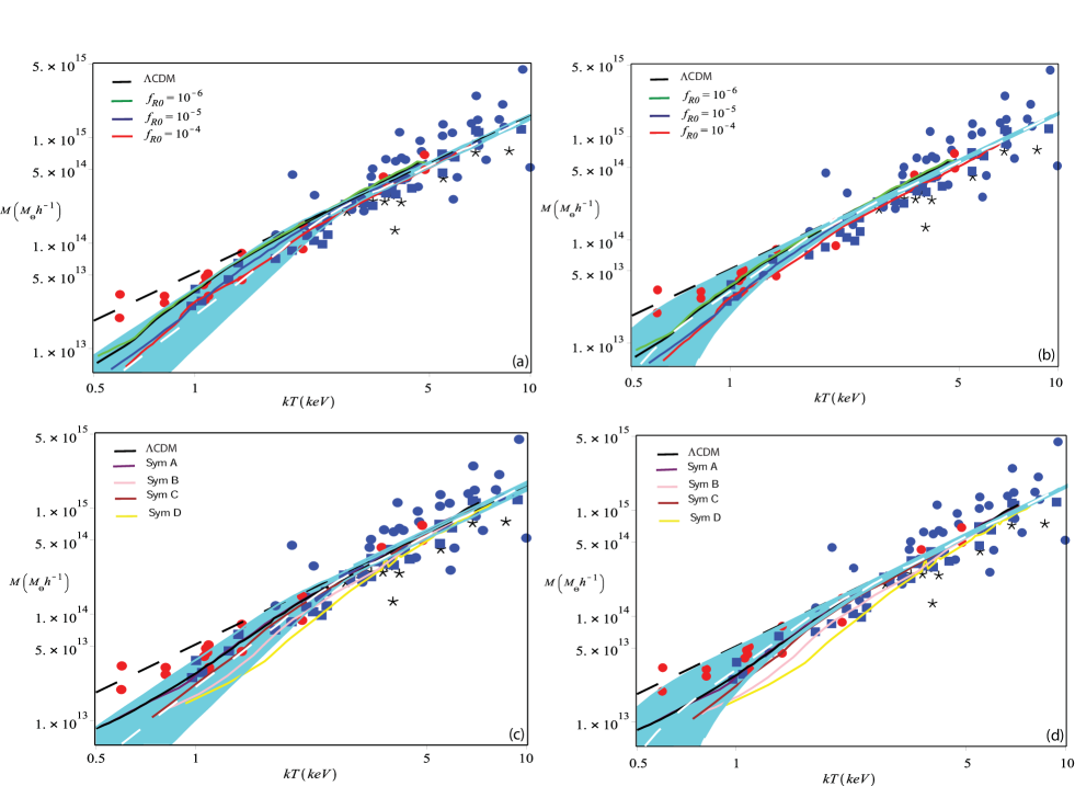
Figure 1: The MTR for $f(R)$ (top panels) and symmetron models (bottom panels). In all the panels, the black line shows the $\Lambda$CDM model, and the dashed black line shows the MTR $\propto T^{3/2}$ as obtained from scaling relations, while the stacked galaxy clusters are depicted with red and blue circles, blue squares, and black stars. In panel (a) (top left) and in (b) (top right), the cyan region shows the 68% confidence level region, obtained using the continuous formation model [Eq. (35)] and the model by Ref. (Afshordi and Cen, 2002) [Eq. (39)], respectively. The white dashed line is the average value. The red, blue, and green lines represent the $f(R)$ model with three different normalizations. Panels (c) (bottom left) and (d) (bottom right) are the equivalent of (a) and (b) for the symmetron models.

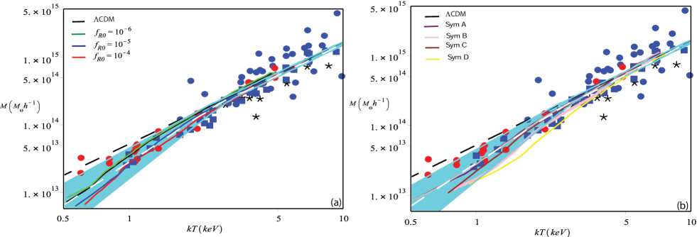
Figure 2: The MTR for $f(R)$ (left panel) and symmetron models (right panel). Lines and symbols represent the same quantities as in Fig. 1, but now the cyan region is the 68% confidence level region, obtained by means of the improved top-hat model [Eq. (24)].

In Fig. 1, we show the results of the comparison between our continuous formation model [Eq. (35)] and the model by Ref. (Afshordi and Cen, 2002) with that of Hammami and Mota (2017) for $f(R)$ and symmetron models. For $f(R)$ models, we consider $n=1$ and $|f_{R0}|=10^{-4},10^{-5},10^{-6}$, while for the symmetron model $(\beta,a_{\rm SSB},\lambda_{0})=(1.0,0.5,1.0)$ for Sym A, (1.0, 0.33, 1.0) for Sym B, (2.0, 0.5, 1.0) for Sym C, and (1.0, 0.25, 1.0) for Sym D.

In all the panels, the black straight dashed line represents the classical MTR self-similar behavior and the black solid line the $\Lambda$CDM model obtained in the simulations of Ref. Hammami and Mota (2017) and for the specific modified gravity models we refer to the caption of Fig. 1. Observational data are represented by points. Red circles come from Ref. (Dai et al., 2007), while blue points are from Ref. (Horner et al., 1999). Stars are from Ref. (Horner et al., 1999) and represent data using spatially resolved observations.

Fig. 1(a) (top left panel) compares the result of our continuous formation model for the $f(R)$ models presented in Ref. Hammami and Mota (2017) (HM). The cyan band represents the 68% confidence level region, obtained using the continuous formation model [Eq. (35)] and calculated similarly to Ref. (Afshordi and Cen, 2002) (Sec. 3.7). The white dashed line is the average value. As expected, deviations from the $\Lambda$CDM model are larger for the model with $f_{R0}=-10^{-4}$, as it represents the model with the strongest modifications to gravity. For smaller values of $f_{R0}$, at temperatures $T<1~{}{\rm keV}$, data are in partial agreement with both the $f(R)$ cosmology and the model presented in this work.

Data points have a large dispersion and circumscribe the theoretical models at high mass, while at the lowest masses data have a value larger than the simulated HM models and the result of our model. Stars show lower masses than the models considered. At high mass, all models are indistinguishable, while at small masses differences become visible.

This is because effects of modified gravity depend on the environment and, hence, on the density. In high-density regions, screening takes place and deviations from $\Lambda$CDM are smaller. Therefore, in high-density regions the $\Lambda$CDM MTR has a similar behavior to that of modified gravity models.

Our model shows a non-self-similar behavior and presents a break at $T\simeq 3$ keV. At small masses, the slope of the central (average) curve, in the range 0.5-3 keV, is $\simeq 2.3$, and the cyan region has an inner and outer slope of $1.8$ and $3$, respectively. The quoted bend has been observed in the literature by several authors (see, e.g. (Finoguenov et al., 2001)), who, assuming the cluster temperature to be constant after the formation time, explained the break as due to the formation redshift. Another possibility is that the cluster medium is preheated in the early phase of formation (Xu et al., 2001). Reference (Afshordi and Cen, 2002), instead, justified the break with the scatter in the density field. The result of the model of Ref. (Afshordi and Cen, 2002) is shown in Fig. 1(b) (top right panel), where once again the cyan region represents the 68% confidence level region, (see Ref. (Afshordi and Cen, 2002), Sec. 3.7).

This model is not able to distinguish between the effect of formation redshift from scatter in the initial energy of the cluster or its initial nonsphericity. However, the presence of nonsphericity gives rise to a mass-dependent asymmetric scatter in the MTR. This scatter is larger than that of the density field and at small temperatures covers all clusters except one, while the bend in the curve of Ref. (Afshordi and Cen, 2002) takes place almost at the same temperature, $T_{X}\simeq 3$ keV, in our model.

In our model, the bend is due to tidal interactions with neighboring clusters, arising from the asphericity of clusters (see (Del Popolo and Gambera, 1999) for a discussion on the relation between angular momentum acquisition, asphericity, and structure formation), and to the effect of dynamical friction. Asphericity gives rise to a mass-dependent asymmetric bend in the MTR. The lower the mass, the larger the difference from the classical self-similar solution. The origin of the bend is due to a few reasons. Our MTR, differently from others (e.g., (Voit, 2000; Afshordi and Cen, 2002)), contains a mass-dependent angular momentum, $L$, originating from the quadrupole moment of the protocluster with the tidal field of the neighboring objects. The presence of this additive mass-dependent term breaks the self-similarity of the MTR. To be more precise, the collapse in our model is different from the THM: The turnaround epoch and collapse time change, as well as the collapse threshold $\delta_{\rm c}$, which is now mass dependent and a monotonic decreasing function of the mass (see Fig. 1 in Ref. (Del Popolo et al., 2017)). It is larger than the standard value at galactic masses and tends to the standard value when we move to the largest clusters. The temperature is $T\propto\epsilon\propto\delta_{\rm c}$ (see (Voit, 2000)), and then less massive clusters are hotter than more massive ones, which are characterized by a standard MTR.

Besides the effect of angular momentum in changing the shape of the MTR, we must recall that another factor contributing is the modification of the partition of energy in virial equilibrium, which influences the shape of the MT relation. At the same time, an important role is played by the cosmological constant and dynamical friction. Both effects, similarly to that of angular momentum, delay the collapse of the perturbation. A comparison of the three effects, the three terms in Eq. (11), are shown in Fig. 1 of Ref. (Del Popolo et al., 2017) and in Fig. 11 of Ref. (Del Popolo, 2009). They are all of the same order of magnitude with differences of a few percent. The effect of dynamical friction (DF) was calculated as shown in Refs. (Antonuccio-Delogu and Colafrancesco, 1994; Del Popolo, 2006, 2009).

The first calculations of the role of DF in clusters formation is due to Refs. (White, 1976; Kashlinsky, 1984, 1986, 1987), who considered the DF generated by the galactic population on the motion of galaxies themselves. Reference (Antonuccio-Delogu and Colafrancesco, 1994) took into account also the effects of substructure and showed DF produces a collapse delay in the collapse of low-$\nu$ peaks, with several consequences, like the mass accumulated by the peak, and similarly to tidal torques.

As a consequence of dynamical friction and tidal torques, one expects changes in the threshold of collapse, the temperature at a given mass (since $T\propto\delta_{\rm c}$), the mass function, and the correlation function. DF and angular momentum have similar effects on structure formation: They delay the collapse, and have similar consequences on the collapse threshold.

An important result of the previous calculation is that the MTR in modified gravity cannot be distinguished from that predicted by the $\Lambda$CDM model. In HM, the MTR in modified gravity was very different from that of $\Lambda$CDM prediction for colder clusters and indistinguishable for hotter ones. Our plots show that the MTR bends in a similar way as done by the MTR in the $f(R)$ models and symmetron models (see the following). The bending was explained previously, and is related to the effect of several factors as the acquisition of angular momentum through tidal torques, by dynamical friction, and by the cosmological constant.

Our model and the $f(R)$ and symmetron models (see the following) of Ref. Hammami and Mota (2017) are in agreement with data till $\simeq 1$ keV; at lower temperatures, a discrepancy is observed with the few clusters present. A similar result is found comparing the $f(R)$ models with the model by (Afshordi and Cen, 2002), in Fig. 1(b). In this case, while $f(R)$ models are in disagreement with the data at small masses, this is no longer true for the model by Ref. (Afshordi and Cen, 2002) and $\Lambda$CDM. However, there is a slight disagreement between the model with $f_{R0}=-10^{-4}$ and Ref. (Afshordi and Cen, 2002).

In particular, in the case of the $f(R)$ models, Figs. 1(a) and 1(b) show that our model is in agreement with all $f(R)$ models considered. In Fig. 1(b), the slope of the average value, in the range 0.5-3 keV, is $\simeq 2.3$, while that of the inner cyan region $\simeq 1.8$ and that of the outer cyan region $>3$ for temperatures $<1$ keV.

Fig. 1(c) shows the same quantities plotted in Figs. 1(a) and 1(b) but for the symmetron case. The plot shows that model Sym D is the one which deviates the most from the $\Lambda$CDM, followed by Sym C, Sym B, and Sym A. Again, at high mass, till $\simeq 4$ keV, our model, the symmetron models and the data are indistinguishable, but Sym D, even if in agreement with the data till $\simeq 3$ keV, slightly differs from our model, namely, with the $\Lambda$CDM predictions. The discrepancy goes on till $\simeq 2$ keV and then disappears. All the other symmetron models are in agreement with our model. As in Fig. 1(a), for $T\leq 1$ keV, the models are in disagreement with a few clusters. Notice that in Figs. 1(a) and 1(c), we compare the continuous formation model with the $f(R)$ and symmetron model, respectively, and then the only change between the two plots is due to the $f(R)$ and symmetron curves. The slopes are then the same as in Fig. 1(a).

Finally, in Fig. 1(d), we show the same results as in Fig. 1(c) but for the model by Ref. (Afshordi and Cen, 2002). The result is similar to Fig. 1(b). In this case, in the range $1\leq T/{\rm keV}\leq 4$, the model by Ref. (Afshordi and Cen, 2002) differs from Sym B and D.

The larger discrepancy between the model by Ref. (Afshordi and Cen, 2002) and the symmetron models in the temperature range 1-4 keV with respect to the predictions of our model is probably due to the fact that, as stressed by Ref. (Afshordi and Cen, 2002), the calculation of the effects of the nonspherical shape of the initial protocluster are not very rigorous and should be considered as an estimate of the actual corrections. The previous assertion is somehow confirmed by the fact that in the given range there is not a real discrepancy between cluster data and the other models (except with the model by Ref. (Afshordi and Cen, 2002)).

We want to stress that the quoted discrepancies between $\Lambda$CDM predictions and Sym B and D, however, do not imply that the symmetron model can be used to claim the MTR is a probe to distinguish between modified gravity and $\Lambda$CDM, since in the quoted temperature range there are no visible peculiar differences between the cluster data and the model.

As before, we stress that Figs. 1(d) and 1(b) differ only for the curves relative to the $f(R)$ and symmetron models, since we are comparing the last with the same model, namely Ref. (Afshordi and Cen, 2002) [Eq. (39)]. The slopes are then the same as in Fig. 1(b).

Finally in Figs. 2(a) and 2(b) we compare the results of the improved top-hat model [Eq. 24)] with the $f(R)$ [Fig. 2(a)] and the symmetron models [Fig. 2(b)] of Ref. (Hammami and Mota, 2017). The results are similar to those plotted in Figs. 1(a) and 1(c), with the difference that the slope discussed previously is now smaller. The differences between the model plotted in Figs. 1(a) and 1(c) (revised top hat) and that in Figs. 2(a) and 2(b) (continuous formation model) are due to the assumed redshift of formation in the two models. The slope of the average curve is $\simeq 2$, and those of the outer and inner cyan region, $\simeq 1.8$, and $\simeq 2.5$, respectively.

Before concluding, we want to add a note on the redshift dependence of the observed cluster data and the MTR which depends on the redshift. All the quantities involved in the determination are, formally, time dependent (concentration and temperature). Therefore, when evaluating the MTR, one has to be cautious and aware of this, as the time evolution can have a substantial effect on the final result. Nevertheless, in our discussion, redshift evolution is not a concern as all the objects considered in Refs. Dai et al. (2007); Horner et al. (1999) are nearby ($z\lesssim 0.2$) and neglecting it has a very small impact when compared to the observational error bars on the mass and temperature.

V Conclusions

In the present work, we derived the MTR relationship using an improved top-hat model and a continuous formation model and compared the results with the prediction of Ref. Hammami and Mota (2017) using $f(R)$ and symmetron models. Our model takes into account dynamical friction, the angular momentum acquired through tidal-torque interaction between clusters, and a modified version of the virial theorem including an external pressure. The continuous formation model is based on the merging-halo formalism by Ref. Lacey and Cole (1993). Both models give a MTR different from the classical self-similar behavior, with a break at 3-4 keV, and a steepening with a decreasing cluster temperature. The comparison of the quoted MTR with those obtained by Ref. Hammami and Mota (2017) for $f(R)$ gravity and symmetron models shows that the MTR is not a good probe to test gravity theories, since the MTR for the $\Lambda$CDM model has the same behavior of that obtained by Ref. Hammami and Mota (2017) for the two modified gravity theories considered.

References

- Bull et al. (2016) P. Bull, Y. Akrami, J. Adamek, T. Baker, E. Bellini, J. Beltrán Jiménez, E. Bentivegna, S. Camera, S. Clesse, J. H. Davis, E. Di Dio, J. Enander, A. Heavens, L. Heisenberg, B. Hu, C. Llinares, R. Maartens, E. Mörtsell, S. Nadathur, J. Noller, R. Pasechnik, M. S. Pawlowski, T. S. Pereira, M. Quartin, A. Ricciardone, S. Riemer-Sørensen, M. Rinaldi, J. Sakstein, I. D. Saltas, V. Salzano, I. Sawicki, A. R. Solomon, D. Spolyar, G. D. Starkman, D. Steer, I. Tereno, L. Verde, F. Villaescusa-Navarro, M. von Strauss, and H. A. Winther, Physics of the Dark Universe 12, 56 (2016), arXiv:1512.05356 .
- Del Popolo (2014) A. Del Popolo, International Journal of Modern Physics D 23, 1430005 (2014), arXiv:1305.0456 [astro-ph.CO] .
- Bertone et al. (2005) G. Bertone, D. Hooper, and J. Silk, Physics Reports 405, 279 (2005), arXiv:hep-ph/0404175 .
- Battistelli et al. (2016) E. S. Battistelli, C. Burigana, P. de Bernardis, A. A. Kirillov, G. B. L. Neto, S. Masi, H. U. Norgaard-Nielsen, P. Ostermann, M. Roman, P. Rosati, and M. Rossetti, International Journal of Modern Physics D 25, 1630023 (2016), arXiv:1609.01110 .
- Bouchet (2004) F. R. Bouchet, Astrophysics and Space Science 290, 69 (2004).
- Kilbinger (2015) M. Kilbinger, Reports on Progress in Physics 78, 086901 (2015), arXiv:1411.0115 .
- Del Popolo (2007) A. Del Popolo, Astronomy Reports 51, 169 (2007), arXiv:0801.1091 .
- Einasto (2001) J. Einasto, Historical Development of Modern Cosmology, Astronomical Society of the Pacific Conference Series, 252, 85 (2001), astro-ph/0012161 .
- Klasen et al. (2015) M. Klasen, M. Pohl, and G. Sigl, Progress in Particle and Nuclear Physics 85, 1 (2015), arXiv:1507.03800 [hep-ph] .
- Riess et al. (1998) A. G. Riess, A. V. Filippenko, P. Challis, and et al., AJ 116, 1009 (1998), arXiv:astro-ph/9805201 .
- Astashenok and del Popolo (2012) A. V. Astashenok and A. del Popolo, Classical and Quantum Gravity 29, 085014 (2012), arXiv:1203.2290 [gr-qc] .
- Velten et al. (2014) H. E. S. Velten, R. F. vom Marttens, and W. Zimdahl, European Physical Journal C 74, 3160 (2014), arXiv:1410.2509 .
- Weinberg (1989) S. Weinberg, Reviews of Modern Physics 61, 1 (1989).
- Spergel et al. (2003) D. N. Spergel, L. Verde, H. V. Peiris, E. Komatsu, M. R. Nolta, C. L. Bennett, M. Halpern, G. Hinshaw, N. Jarosik, A. Kogut, M. Limon, S. S. Meyer, L. Page, G. S. Tucker, J. L. Weiland, E. Wollack, and E. L. Wright, ApJS 148, 175 (2003), astro-ph/0302209 .
- Komatsu et al. (2011) E. Komatsu, K. M. Smith, J. Dunkley, and et al., ApJS 192, 18 (2011), arXiv:1001.4538 [astro-ph.CO] .
- Moore et al. (1999) B. Moore, T. Quinn, F. Governato, J. Stadel, and G. Lake, MNRAS 310, 1147 (1999), astro-ph/9903164 .
- de Blok (2010) W. J. G. de Blok, Advances in Astronomy 2010, 789293 (2010), arXiv:0910.3538 .
- Ostriker and Steinhardt (2003) J. P. Ostriker and P. Steinhardt, Science 300, 1909 (2003), astro-ph/0306402 .
- Boylan-Kolchin et al. (2011) M. Boylan-Kolchin, J. S. Bullock, and M. Kaplinghat, MNRAS 415, L40 (2011), arXiv:1103.0007 [astro-ph.CO] .
- Del Popolo and Hiotelis (2014) A. Del Popolo and N. Hiotelis, JCAP 1, 047 (2014), arXiv:1401.6577 [astro-ph.GA] .
- Del Popolo and Le Delliou (2014) A. Del Popolo and M. Le Delliou, JCAP 12, 051 (2014), arXiv:1408.4893 .
- Del Popolo and Le Delliou (2017) A. Del Popolo and M. Le Delliou, Galaxies 5, 17 (2017), arXiv:1606.07790 .
- Eriksen et al. (2004) H. K. Eriksen, F. K. Hansen, A. J. Banday, K. M. Górski, and P. B. Lilje, ApJ 605, 14 (2004), astro-ph/0307507 .
- Schwarz et al. (2004) D. J. Schwarz, G. D. Starkman, D. Huterer, and C. J. Copi, Physical Review Letters 93, 221301 (2004), astro-ph/0403353 .
- Cruz et al. (2005) M. Cruz, E. Martínez-González, P. Vielva, and L. Cayón, MNRAS 356, 29 (2005), astro-ph/0405341 .
- Copi et al. (2006) C. J. Copi, D. Huterer, D. J. Schwarz, and G. D. Starkman, MNRAS 367, 79 (2006), astro-ph/0508047 .
- Macaulay et al. (2013) E. Macaulay, I. K. Wehus, and H. K. Eriksen, Physical Review Letters 111, 161301 (2013), arXiv:1303.6583 .
- Planck Collaboration XVI (2014) Planck Collaboration XVI, A&A 571, A16 (2014), arXiv:1303.5076 [astro-ph.CO] .
- Raveri (2016) M. Raveri, Phys. Rev. D 93, 043522 (2016), arXiv:1510.00688 .
- Zentner and Bullock (2003) A. R. Zentner and J. S. Bullock, ApJ 598, 49 (2003), astro-ph/0304292 .
- Brooks et al. (2013) A. M. Brooks, M. Kuhlen, A. Zolotov, and D. Hooper, ApJ 765, 22 (2013), arXiv:1209.5394 .
- Oñorbe et al. (2015) J. Oñorbe, M. Boylan-Kolchin, J. S. Bullock, P. F. Hopkins, D. Kerěs, C.-A. Faucher-Giguère, E. Quataert, and N. Murray, ArXiv e-prints (2015), arXiv:1502.02036 .
- El-Zant et al. (2001) A. El-Zant, I. Shlosman, and Y. Hoffman, ApJ 560, 636 (2001), astro-ph/0103386 .
- El-Zant et al. (2004) A. A. El-Zant, Y. Hoffman, J. Primack, F. Combes, and I. Shlosman, ApJL 607, L75 (2004), astro-ph/0309412 .
- Del Popolo (2009) A. Del Popolo, ApJ 698, 2093 (2009), arXiv:0906.4447 [astro-ph.CO] .
- Nipoti and Binney (2015) C. Nipoti and J. Binney, MNRAS 446, 1820 (2015), arXiv:1410.6169 .
- Del Popolo and Pace (2016) A. Del Popolo and F. Pace, Astrophysics and Space Science 361, 162 (2016), arXiv:1502.01947 .
- Bekenstein (2010) J. D. Bekenstein, “Modified gravity as an alternative to dark matter,” in Particle Dark Matter : Observations, Models and Searches, edited by G. Bertone (Cambridge University Press, 2010) p. 99.
- Joyce et al. (2016) A. Joyce, L. Lombriser, and F. Schmidt, Annual Review of Nuclear and Particle Science 66, 95 (2016), arXiv:1601.06133 .
- Starobinskiǐ (1979) A. A. Starobinskiǐ, Soviet Journal of Experimental and Theoretical Physics Letters 30, 682 (1979).
- Guth (1981) A. H. Guth, Phys. Rev. D 23, 347 (1981).
- Milgrom (1983) M. Milgrom, ApJ 270, 365 (1983).
- Moffat (2006) J. W. Moffat, JCAP 3, 004 (2006), gr-qc/0506021 .
- De Felice and Tsujikawa (2010) A. De Felice and S. Tsujikawa, Living Reviews in Relativity 13, 3 (2010), arXiv:1002.4928 [gr-qc] .
- Armendariz-Picon et al. (2001) C. Armendariz-Picon, V. Mukhanov, and P. J. Steinhardt, Phys. Rev. D 63, 103510 (2001), arXiv:astro-ph/0006373 .
- Kamenshchik et al. (2001) A. Kamenshchik, U. Moschella, and V. Pasquier, Physics Letters B 511, 265 (2001), arXiv:gr-qc/0103004 .
- de Putter and Linder (2007) R. de Putter and E. V. Linder, Astroparticle Physics 28, 263 (2007), arXiv:0705.0400 .
- Durrer (2008) R. Durrer, The Cosmic Microwave Background by Ruth Durrer. Cambridge Catalogue, September 2008., edited by Durrer, R. (2008).
- Dvali et al. (2000) G. Dvali, G. Gabadadze, and M. Porrati, Physics Letters B 485, 208 (2000), arXiv:hep-th/0005016 .
- Linder (2010) E. V. Linder, Phys. Rev. D 81, 127301 (2010), arXiv:1005.3039 [astro-ph.CO] .
- Milgrom (2014) M. Milgrom, Phys. Rev. D 89, 024027 (2014), arXiv:1308.5388 [gr-qc] .
- Bekenstein (2004) J. D. Bekenstein, Phys. Rev. D 70, 083509 (2004), astro-ph/0403694 .
- Zwiebach (1985) B. Zwiebach, Physics Letters B 156, 315 (1985).
- Nojiri et al. (2005) S. Nojiri, S. D. Odintsov, and M. Sasaki, Phys. Rev. D 71, 123509 (2005), hep-th/0504052 .
- Lovelock (1971) D. Lovelock, Journal of Mathematical Physics 12, 498 (1971).
- Hořava (2009) P. Hořava, Phys. Rev. D 79, 084008 (2009), arXiv:0901.3775 [hep-th] .
- Rodríguez and Navarro (2017) Y. Rodríguez and A. A. Navarro, in Journal of Physics Conference Series, Journal of Physics Conference Series, Vol. 831 (2017) p. 012004, arXiv:1703.01884 [hep-th] .
- Horndeski (1974) G. W. Horndeski, International Journal of Theoretical Physics 10, 363 (1974).
- Deffayet et al. (2010) C. Deffayet, O. Pujolàs, I. Sawicki, and A. Vikman, JCAP 10, 026 (2010), arXiv:1008.0048 [hep-th] .
- Debono and Smoot (2016) I. Debono and G. F. Smoot, Universe 2, 23 (2016), arXiv:1609.09781 [gr-qc] .
- Ni (1972) W.-T. Ni, ApJ 176, 769 (1972).
- Will (1993) C. M. Will, Theory and Experiment in Gravitational Physics, by Clifford M. Will, pp. 396. ISBN 0521439736. Cambridge, UK: Cambridge University Press, March 1993. (1993) p. 396.
- Bertotti et al. (2003) B. Bertotti, L. Iess, and P. Tortora, Nature (London) 425, 374 (2003).
- Will (2014) C. M. Will, Living Reviews in Relativity 17, 4 (2014), arXiv:1403.7377 [gr-qc] .
- Dupé et al. (2011) F.-X. Dupé, A. Rassat, J.-L. Starck, and M. J. Fadili, A&A 534, A51 (2011), arXiv:1010.2192 .
- (66) http://www.euclid-ec.org.
- (67) http://jdem.lbl.gov/.
- (68) https://www.skatelescope.org.
- (69) https://www.lsst.org.
- Battye et al. (2018) R. A. Battye, B. Bolliet, and F. Pace, Phys. Rev. D 97, 104070 (2018), arXiv:1712.05976 .
- Battye et al. (2019) R. A. Battye, B. Bolliet, F. Pace, and D. Trinh, Phys. Rev. D 99, 043515 (2019).
- Dimopoulos et al. (2007) S. Dimopoulos, P. W. Graham, J. M. Hogan, and M. A. Kasevich, Physical Review Letters 98, 111102 (2007), gr-qc/0610047 .
- Brax et al. (2012) P. Brax, A.-C. Davis, B. Li, and H. A. Winther, Phys. Rev. D 86, 044015 (2012), arXiv:1203.4812 [astro-ph.CO] .
- Hammami and Mota (2017) A. Hammami and D. F. Mota, A&A 598, A132 (2017), arXiv:1603.08662 .
- Hu and Sawicki (2007) W. Hu and I. Sawicki, Phys. Rev. D 76, 064004 (2007), arXiv:0705.1158 .
- Hinterbichler and Khoury (2010) K. Hinterbichler and J. Khoury, Physical Review Letters 104, 231301 (2010), arXiv:1001.4525 [hep-th] .
- Llinares et al. (2008) C. Llinares, A. Knebe, and H. Zhao, MNRAS 391, 1778 (2008), arXiv:0809.2899 .
- Zhao et al. (2011) G.-B. Zhao, B. Li, and K. Koyama, Phys. Rev. D 83, 044007 (2011), arXiv:1011.1257 [astro-ph.CO] .
- Puchwein et al. (2013) E. Puchwein, M. Baldi, and V. Springel, MNRAS 436, 348 (2013), arXiv:1305.2418 .
- Llinares et al. (2014) C. Llinares, D. F. Mota, and H. A. Winther, A&A 562, A78 (2014), arXiv:1307.6748 .
- Gronke et al. (2014) M. B. Gronke, C. Llinares, and D. F. Mota, A&A 562, A9 (2014), arXiv:1307.6994 .
- Bhattacharya et al. (2017) S. Bhattacharya, K. F. Dialektopoulos, A. Enea Romano, C. Skordis, and T. N. Tomaras, JCAP 7, 018 (2017), arXiv:1611.05055 .
- Lopes et al. (2018) R. C. C. Lopes, R. Voivodic, L. R. Abramo, and L. Sodré, Jr., JCAP 9, 010 (2018), arXiv:1805.09918 .
- Adhikari et al. (2018) S. Adhikari, J. Sakstein, B. Jain, N. Dalal, and B. Li, JCAP 11, 033 (2018), arXiv:1806.04302 .
- Del Popolo (2002) A. Del Popolo, A&A 387, 759 (2002), astro-ph/0202436 .
- Martel and Shapiro (1998) H. Martel and P. R. Shapiro, MNRAS 297, 467 (1998), astro-ph/9710119 .
- Hammami and Mota (2015) A. Hammami and D. F. Mota, A&A 584, A57 (2015), arXiv:1505.06803 .
- Voit and Donahue (1998) G. M. Voit and M. Donahue, ApJL 500, L111 (1998), astro-ph/9804306 .
- Voit (2000) G. M. Voit, ApJ 543, 113 (2000), astro-ph/0006366 .
- Afshordi and Cen (2002) N. Afshordi and R. Cen, ApJ 564, 669 (2002), astro-ph/0105020 .
- Del Popolo et al. (2005) A. Del Popolo, N. Hiotelis, and J. Peñarrubia, ApJ 628, 76 (2005), arXiv:astro-ph/0508596 [astro-ph] .
- Del Popolo and Gambera (1999) A. Del Popolo and M. Gambera, A&A 344, 17 (1999), arXiv:astro-ph/9806044 .
- Lacey and Cole (1993) C. Lacey and S. Cole, MNRAS 262, 627 (1993).
- Peebles (1993) P. J. E. Peebles, Princeton Series in Physics, Princeton, NJ: Princeton University Press, —c1993, edited by P. J. E. Peebles (1993).
- Bartlett and Silk (1993) J. G. Bartlett and J. Silk, ApJL 407, L45 (1993).
- Lahav et al. (1991) O. Lahav, P. B. Lilje, J. R. Primack, and M. J. Rees, MNRAS 251, 128 (1991).
- Del Popolo and Gambera (1998) A. Del Popolo and M. Gambera, A&A 337, 96 (1998), astro-ph/9802214 .
- Fosalba and Gaztan̈aga (1998) P. Fosalba and E. Gaztan̈aga, MNRAS 301, 503 (1998), arXiv:astro-ph/9712095 .
- Engineer et al. (2000) S. Engineer, N. Kanekar, and T. Padmanabhan, MNRAS 314, 279 (2000), astro-ph/9812452 .
- Del Popolo et al. (2013) A. Del Popolo, F. Pace, and J. A. S. Lima, MNRAS 430, 628 (2013), arXiv:1212.5092 [astro-ph.CO] .
- Pace et al. (2018) F. Pace, C. Schimd, D. F. Mota, and A. Del Popolo, arXiv e-prints (2018), arXiv:1811.12105 .
- Pace et al. (2010) F. Pace, J.-C. Waizmann, and M. Bartelmann, MNRAS 406, 1865 (2010), arXiv:1005.0233 [astro-ph.CO] .
- Pace et al. (2017) F. Pace, S. Meyer, and M. Bartelmann, JCAP 10, 040 (2017), arXiv:1708.02477 .
- Barbosa et al. (2015) C. M. S. Barbosa, J. C. Fabris, O. F. Piattella, H. E. S. Velten, and W. Zimdahl, arXiv e-prints (2015), arXiv:1512.00921 .
- Landau and Lifshitz (1966) L. D. Landau and E. M. Lifshitz, Lehrbuch der theoretischen Physik, Berlin: Akademie-Verlag, 1966, 4. Auflage (1966).
- Shapiro et al. (1999) P. R. Shapiro, I. T. Iliev, and A. C. Raga, MNRAS 307, 203 (1999), arXiv:astro-ph/9810164 [astro-ph] .
- Iliev and Shapiro (2001) I. T. Iliev and P. R. Shapiro, MNRAS 325, 468 (2001), astro-ph/0101067 .
- Lilje (1992) P. B. Lilje, ApJL 386, L33 (1992).
- Colafrancesco et al. (1995) S. Colafrancesco, V. Antonuccio-Delogu, and A. Del Popolo, ApJ 455, 32 (1995), astro-ph/9410093 .
- Kitayama and Suto (1996) T. Kitayama and Y. Suto, ApJ 469, 480 (1996), astro-ph/9604141 .
- Viana and Liddle (1996) P. T. P. Viana and A. R. Liddle, MNRAS 281, 323 (1996), arXiv:astro-ph/9511007 .
- Dai et al. (2007) X. Dai, C. S. Kochanek, and N. D. Morgan, ApJ 658, 917 (2007), astro-ph/0606002 .
- Horner et al. (1999) D. J. Horner, R. F. Mushotzky, and C. A. Scharf, ApJ 520, 78 (1999), astro-ph/9902151 .
- Finoguenov et al. (2001) A. Finoguenov, T. H. Reiprich, and H. Böhringer, A&A 368, 749 (2001), arXiv:astro-ph/0010190 .
- Xu et al. (2001) H. Xu, G. Jin, and X.-P. Wu, ApJ 553, 78 (2001), astro-ph/0101564 .
- Del Popolo et al. (2017) A. Del Popolo, F. Pace, and M. Le Delliou, JCAP 3, 032 (2017), arXiv:1703.06918 .
- Antonuccio-Delogu and Colafrancesco (1994) V. Antonuccio-Delogu and S. Colafrancesco, ApJ 427, 72 (1994).
- Del Popolo (2006) A. Del Popolo, A&A 454, 17 (2006), arXiv:0801.1086 .
- White (1976) S. D. M. White, MNRAS 174, 19 (1976).
- Kashlinsky (1984) A. Kashlinsky, MNRAS 208, 623 (1984).
- Kashlinsky (1986) A. Kashlinsky, ApJ 306, 374 (1986).
- Kashlinsky (1987) A. Kashlinsky, ApJ 312, 497 (1987).