Cost Reduction of Swapping Bonds Part in Anisotropic Tensor Renormalization Group

Abstract

The bottleneck part of anisotropic tensor renormalization group (ATRG) is a swapping bonds part which consists of a contraction of two tensors and a partial singular value decomposition of a matrix, and their computational costs are $O(\chi^{2d+1})$, where $\chi$ is the maximum bond dimension and $d$ is the dimensionality of a system. We propose an alternative method for the swapping bonds part and it scales with $O(\chi^{\max(d+3,7)})$, though the total cost of ATRG with the method remains $O(\chi^{2d+1})$. Moreover, the memory cost of the whole algorithm can be reduced from $O(\chi^{2d})$ to $O(\chi^{\max(d+1,6)})$. We examine ATRG with or without the proposed method in the four-dimensional Ising model and find that the free energy density of the proposed algorithm is consistent with that of the original ATRG while the elapsed time is significantly reduced. We also compare the proposed algorithm with higher-order tensor renromalization group (HOTRG) and find that the value of the free energy density of the proposed algorithm is lower than that of HOTRG in the fixed elapsed time.

I Introduction

Tensor network algorithms are theoretically and numerically useful tools for quantum and classical many-body systems Intro_TN_1 ; Intro_TN_2 . For example, to study a one-dimensional quantum many-body system, one can use density matrix renormalization group DMRG ; DMRG_PRB ; DMRGreview , which is based on matrix product states MPS_1 ; MPS_2 and can be understood as a variational method for a wave function. For higher dimensional cases, there are algorithms based on projected entangled pair states PEPS ; PEPS_2 ; PEPS_3 . In addition to those algorithms, tensor renormalization group (TRG) TRG is an approach for coarse-graining tensor networks and calculates the partition function of a two dimensional classical model. For studying two or higher dimensional classical systems, we can use higher-order tensor renormalization group (HOTRG) HOTRG . There are series of the improved algorithms for the coarse graining on the basis of various philosophies SRG ; TEFR ; TNR ; TNR_PRB ; loopTNR ; hamiltonian_TRG ; RSVDTRG ; Gilt ; EBO ; FET ; PTTRG ; BTRG ; ATRG .

Since the tensor network algorithms avoid the sign problem, they have received attention not only from condensed matter physics but also from high energy physics Banuls:2013jaa ; Kuhn:2015zqa ; Banuls:2015sta ; Banuls:2016lkq ; Banuls:2016gid ; Banuls:2017ena ; Shimizu:2012zza ; Shimizu:2014uva ; Shimizu:2014fsa ; Shimizu:2017onf ; Denbleyker:2013bea ; Yu:2013sbi ; Meurice:2016mkb ; Takeda:2014vwa ; Kawauchi:2016xng ; Sakai:2017jwp ; Kadoh:2018hqq . We hope that the lattice models suffering from the sign problem in high energy physics, (such as quantum chromodynamics with finite quark density, the $\theta$ vacuum of quantum chromodynamics, chiral gauge theory and the super-symmetric model) can be analyzed by the tensor network algorithms. However, if one computes physical quantities of such high dimensional systems with the algorithms, the computational costs and the memory costs get worse and it is difficult for the algorithms to provide results with sufficient precision.

A novel algorithm, anisotropic tensor renormalization group (ATRG), has been proposed recently ATRG . It is one of the tensor network algorithms for coarse-graining tensor networks and can be applied to an arbitrary dimensional lattice model like HOTRG. Moreover, it takes much lower computational-cost than HOTRG. The bottleneck part in ATRG is a swapping bonds part which consists of a contraction of two tensors and a partial singular value decomposition (PSVD) of a matrix. The computational cost and the memory cost of the part are $O(\chi^{2d+1})$ and $O(\chi^{2d})$ respectively, where $\chi$ is the maximum bond dimension and $d$ is the dimensionality of a system. If the costs of the swapping bonds part in ATRG are reduced, we can expect to obtain more accurate results than those from the original ATRG with the same elapsed time and the same memory resource.

In this paper, we propose a swapping bonds method of which the computational cost can be reduced from $O(\chi^{2d+1})$ to $O(\chi^{\max(d+3,7)})$ and the memory cost of the whole algorithm can be reduced from $O(\chi^{2d})$ to $O(\chi^{\max(d+1,6)})$. Furthermore, we numerically examine the accuracy of the free energy density of the four-dimensional Ising model and the elapsed time of ATRG using the proposed method to compare with the original ATRG and HOTRG.

The rest of this paper is organized as follows. In Sec. II, we review the original ATRG algorithm for a four-dimensional hypercubic system. In Sec. III, the proposed swapping bonds method is explained. In Sec. IV, we present numerical results of the four-dimensional Ising model for a comparison between ATRG with the proposed method and the original ATRG or HOTRG and discuss their performances. A summary and outlooks are given in Sec. V. In appendix A, we explain a method for making tensors, $E$ and $F$, in ATRG. In appendix B, we study the parameters of the randomized singular value decomposition (RSVD).

II Anisotropic Tensor Renormalization Group

In this section, we explain the original ATRG ATRG for a four-dimensional hypercubic system. First of all, we rewrite the partition function of the system in terms of a tensor network as

$$Z=\mathrm{Tr}\prod_{i}T^{(\mathrm{init})}_{i;x_{0}x_{1}y_{0}y_{1}z_{0}z_{1}w_{0}w_{1}},$$ (1)

where $T^{(\mathrm{init})}_{i}$ is an initial tensor, $i$ runs all lattice sites, and $\mathrm{Tr}$ means summing up all the bond indices of the initial tensors. If the direction of the coarse graining is set in $x$-axis , which is the vertical direction in Fig. 1, we redefine the initial tensor as $T^{(\mathrm{init})}_{i;\Omega_{0}\Omega_{1}x_{0}x_{1}}$, where $\Omega_{0}=(y_{0},z_{0},w_{0})$ and $\Omega_{1}=(y_{1},z_{1},w_{1})$ are bundles of the bond indices .

Figure 1: The initial tensor $T^{(\mathrm{init})}_{i}$ in the initial tensor network of a four-dimensional system. (a) We focus on two tensors in the initial tensor network. (b) If the direction of the coarse graining is set in $x$-axis, we redefine the initial tensor as $T^{(\mathrm{init})}_{i;\Omega_{0}\Omega_{1}x_{0}x_{1}}$, where $\Omega_{0}=(y_{0},z_{0},w_{0})$ and $\Omega_{1}=(y_{1},z_{1},w_{1})$ are bundles of the bond indices.

Then, we execute the coarse graining of the tensor network to reduce the degrees of freedom using ATRG ATRG . The whole flow of ATRG is shown in Fig. 2 where there are seven steps, (a)–(g).

Figure 2: The flow of the original ATRG. In step (a), a tensor $T$ is decomposed into two tensors such as $A$ and $B$ or $C$ and $D$ with the SVD. In step (b), the two tensors, $B$ and $C$, are contracted by summing up the bond $x_{1}$ and a tensor $M$ is obtained. In step (c), $M$ is decomposed by the PSVD into two tensors, $X$ and $Y$, to change the combinations of bonds from $\Omega_{1}\alpha$ of $B$ and $\Omega_{2}\beta$ of $C$ to $\Omega_{2}\alpha$ of $X$ and $\Omega_{1}\beta$ of $Y$. In step (d), two tensors, $E$ and $F$, are made from $A,X,Y$ and $D$ with a method is explained in appendix A. In step (e), we contract $A,X$ and $E$ by summing up the bonds $\alpha,\Omega_{0},\Omega_{2}$ to make $G$, and contract $D,Y$ and $F$ by summing up the bonds $\beta,\Omega_{1},\Omega_{3}$ to make $H$. In step (f), $G$ and $H$ are contracted by summing up the bond $x_{1}$ to obtain a coarse-grained tensor $T^{\prime}$. In step (g), we reorder the bonds of $T^{\prime}$ for the next direction of the coarse graining, $y$-axis.

First, in step (a), a tensor $T$ is decomposed with the singular value decomposition (SVD),

$$T_{\Omega_{0}\Omega_{1}x_{0}x_{1}}\simeq\sum_{\alpha=1}^{\chi}U_{\{T\}\Omega_{0}x_{0}\alpha}S_{\{T\}\alpha\alpha}V_{\{T\}\Omega_{1}x_{1}\alpha},$$ (2)

where $\alpha$ is a new bond for $x$-axis. Then, we make four tensors, $A,B,C$ and $D$, as

$$A_{\Omega_{0}x_{0}\alpha} =U_{\{T\}\Omega_{0}x_{0}\alpha},$$ (3)

$$B_{\Omega_{1}x_{1}\alpha} =S_{\{T\}\alpha\alpha}V_{\{T\}\Omega_{1}x_{1}\alpha},$$ (4)

$$C_{\Omega_{0}x_{0}\alpha} =S_{\{T\}\alpha\alpha}U_{\{T\}\Omega_{0}x_{0}\alpha},$$ (5)

$$D_{\Omega_{1}x_{1}\alpha} =V_{\{T\}\Omega_{1}x_{1}\alpha}.$$ (6)

In step (b), the two tensors, $B$ and $C$, are contracted and a tensor $M$ is obtained by

$$M_{\Omega_{1}\Omega_{2}\alpha\beta}=\sum_{x_{1}}B_{\Omega_{1}x_{1}\alpha}C_{\Omega_{2}x_{1}\beta}.$$ (7)

Then in step (c), we decompose $M$ into two tensors, $X$ and $Y$, to change the combinations of the bonds from $\Omega_{1}\alpha$ of $B$ and $\Omega_{2}\beta$ of $C$ to $\Omega_{2}\alpha$ of $X$ and $\Omega_{1}\beta$ of $Y$ as

$$M_{\Omega_{1}\Omega_{2}\alpha\beta} \simeq\sum_{x_{1}=1}^{\chi}U_{\{M\}\Omega_{2}\alpha x_{1}}S_{\{M\}x_{1}x_{1}}V_{\{M\}\Omega_{1}\beta x_{1}},$$ (8)

$$X_{\Omega_{2}\alpha x_{1}} =\sqrt{S_{\{M\}x_{1}x_{1}}}U_{\{M\}\Omega_{2}\alpha x_{1}},$$ (9)

$$Y_{\Omega_{1}\beta x_{1}} =\sqrt{S_{\{M\}x_{1}x_{1}}}V_{\{M\}\Omega_{1}\beta x_{1}}.$$ (10)

One may use the PSVD, such as the Arnoldi method Arnoldi and the RSVD RSVD , for the decomposition of $M$ in eq. (8). In step (d), two tensors, $E$ and $F$, are made from $A,X,Y$ and $D$ with a method explained in appendix A. In step (e), we contract $A,X$ and $E$ to make $G$, and contract $D,Y$ and $F$ to make $H$ as

$$G_{\Omega^{\prime}_{0}x_{0}x_{1}} =\sum_{\alpha,\Omega_{0},\Omega_{2}}A_{\Omega_{0}x_{0}\alpha}X_{\Omega_{2}\alpha x_{1}}E_{\Omega_{0}\Omega_{2}\Omega^{\prime}_{0}},$$ (11)

$$H_{\Omega^{\prime}_{1}x_{1}x_{2}} =\sum_{\beta,\Omega_{1},\Omega_{3}}D_{\Omega_{3}x_{2}\beta}Y_{\Omega_{1}\beta x_{1}}F_{\Omega_{1}\Omega_{3}\Omega^{\prime}_{1}},$$ (12)

where $\Omega^{\prime}_{0}=(y^{\prime}_{0},z^{\prime}_{0},w^{\prime}_{0})$ and $\Omega^{\prime}_{1}=(y^{\prime}_{1},z^{\prime}_{1},w^{\prime}_{1})$. Then, in step (f), $G$ and $H$ are contracted to obtain a coarse-grained tensor $T^{\prime}$,

$$T^{\prime}_{\Omega^{\prime}_{0}\Omega^{\prime}_{1}x_{0}x_{2}}=\sum_{x_{1}}G_{\Omega^{\prime}_{0}x_{0}x_{1}}H_{\Omega^{\prime}_{1}x_{1}x_{2}}.$$ (13)

Finally, in step (g), we reorder the bonds of $T^{\prime}$ for the next direction of the coarse graining, $y$-axis, and redefine $T^{\prime}$ as $T^{\prime}_{\Psi^{\prime}_{0}\Psi^{\prime}_{1}y^{\prime}_{0}y^{\prime}_{1}}$ in the same way as the initial tensor, where $\Psi^{\prime}_{0}=(x_{0},z^{\prime}_{0},w^{\prime}_{0})$ and $\Psi^{\prime}_{1}=(x_{2},z^{\prime}_{1},w^{\prime}_{1})$.

As explained in ATRG , the step (f), (g) and the step (a) of the next coarse graining can be replaced by the following method which has no truncation errors and reduces the computational cost. The flow of the improved method consistis of four steps which are shown in step (c), (d), (e) and (f) of Fig. 3.

Figure 3: The flow of the improved method to make $A^{\prime},B^{\prime},C^{\prime}$ and $D^{\prime}$ from $G$ and $H$ ATRG . Step (a) and (b) represent the step (f), (g) and (a) in Fig. 2. In step (c), $G$ and $H$ are decomposed in the coarse-grained direction to obtain $K$ by the contraction in eq. (16). In step (d), we execute the SVD of $K$. In step (e), $A^{\prime},B^{\prime},C^{\prime}$ and $D^{\prime}$ are made by the contraction in eq. (18)–(21). In step (f), we reorder the bonds of $A^{\prime},B^{\prime},C^{\prime}$ and $D^{\prime}$ for the next coarse graining.

In step (c) of Fig. 3, $G$ and $H$ are decomposed in the coarse-grained direction as

$$G_{\Omega^{\prime}_{0}x_{0}x_{1}} =\sum_{\gamma}U_{\{G\}\Omega^{\prime}_{0}x_{0}\gamma}S_{\{G\}\gamma\gamma}V_{\{G\}x_{1}\gamma},$$ (14)

$$H_{\Omega^{\prime}_{1}x_{1}x_{2}} =\sum_{\delta}U_{\{H\}\Omega^{\prime}_{1}x_{2}\delta}S_{\{H\}\delta\delta}V_{\{H\}x_{1}\delta},$$ (15)

and $S_{\{G\}\gamma\gamma},V_{\{G\}x_{1}\gamma},V_{\{H\}x_{1}\delta}$ and $S_{\{H\}\delta\delta}$ are contracted to obtain $K$,

$$K_{\gamma\delta} =\sum_{x_{1}}S_{\{G\}\gamma\gamma}V_{\{G\}x_{1}\gamma}V_{\{H\}x_{1}\delta}S_{\{H\}\delta\delta}.$$ (16)

In step (d) of Fig. 3, we decompose $K$ with the SVD,

$$K_{\gamma\delta} =\sum_{\alpha}U_{\{K\}\gamma\alpha}S_{\{K\}\alpha\alpha}V_{\{K\}\delta\alpha},$$ (17)

and, in step (e) of Fig. 3, we contract the following tensors to make $A^{\prime},B^{\prime},C^{\prime}$ and $D^{\prime}$,

$$A^{\prime}_{\Omega^{\prime}_{0}x_{0}\alpha} =\sum_{\gamma}U_{\{K\}\gamma\alpha}U_{\{G\}\Omega^{\prime}_{0}x_{0}\gamma},$$ (18)

$$B^{\prime}_{\Omega^{\prime}_{1}x_{2}\alpha} =\sum_{\delta}S_{\{K\}\alpha\alpha}V_{\{K\}\delta\alpha}U_{\{H\}\Omega^{\prime}_{1}x_{2}\delta},$$ (19)

$$C^{\prime}_{\Omega^{\prime}_{0}x_{0}\alpha} =\sum_{\gamma}S_{\{K\}\alpha\alpha}U_{\{K\}\gamma\alpha}U_{\{G\}\Omega^{\prime}_{0}x_{0}\gamma},$$ (20)

$$D^{\prime}_{\Omega^{\prime}_{1}x_{2}\alpha} =\sum_{\delta}V_{\{K\}\delta\alpha}U_{\{H\}\Omega^{\prime}_{1}x_{2}\delta}.$$ (21)

Finally, in step (f), we reorder the bonds of $A^{\prime},B^{\prime},C^{\prime}$ and $D^{\prime}$ for the next coarse graining in a similar way to the step (g) in Fig. 2.

The total computational cost of the original ATRG is $O(\chi^{2d+1})$ and the total memory cost is $O(\chi^{2d})$. The former cost comes from the step (e) in Fig. 2 and the swapping bonds part which consists of the step (b) and the step (c) in Fig. 2. The latter cost arises from the swapping bonds part. Therefore, the swapping bonds part is the bottleneck one of both the computational cost and the memory cost in ATRG.

III Cost reduction of swapping bonds part

In this section we propose a swapping bonds method instead of the step (b) and (c) in Fig. 2. The flow of the proposed method is shown in step (c), (d), (e) and (f) of Fig. 4.

Figure 4: The cost reduction of the swapping bonds part in ATRG. Step (a) and (b) represent the step (b) and (c) of Fig. 2. In step (c), we perform the SVDs of $B$ and $C$ to make $B^{\mathrm{s}}$ and $C^{\mathrm{s}}$ by the contractions in eq. (24) and (25). Note that there is no truncation in this step and the red lines mean that the maximum bond dimensions of the indices, $\mu$ and $\nu$, are taken to be $\chi^{2}$. In step (d), $M^{\mathrm{s}}$ is made of the contraction of $B^{\mathrm{s}}$ and $C^{\mathrm{s}}$ by summing up the bond $x_{1}$. In step (e), the combinations of the bonds are changed from $\mu\alpha$ of $B^{\mathrm{s}}$ and $\beta\nu$ of $C^{\mathrm{s}}$ to $\nu\alpha$ of $X^{\mathrm{s}}$ and $\mu\beta$ of $Y^{\mathrm{s}}$ using the PSVD. In step (f), we contract $X^{\mathrm{s}}$ and $U_{\{C\}}$ by summing up the bonds $\nu$ to make $X$, and contract $Y^{\mathrm{s}}$ and $U_{\{B\}}$ by summing up the bonds $\mu$ to make $Y$.

The first step of the proposed swapping bonds method (step (c) of Fig. 4) is the SVDs of $B$ and $C$ as

$$B_{\Omega_{1}x_{1}\alpha} =\sum_{\mu}U_{\{B\}\Omega_{1}\mu}S_{\{B\}\mu\mu}V_{\{B\}x_{1}\alpha\mu},$$ (22)

$$C_{\Omega_{2}x_{1}\beta} =\sum_{\nu}U_{\{C\}\Omega_{2}\nu}S_{\{C\}\nu\nu}V_{\{C\}x_{1}\beta\nu},$$ (23)

and defining $B^{\mathrm{s}}$ and $C^{\mathrm{s}}$ as

$$B^{\mathrm{s}}_{x_{1}\alpha\mu} =S_{\{B\}\mu\mu}V_{\{B\}x_{1}\alpha\mu},$$ (24)

$$C^{\mathrm{s}}_{x_{1}\beta\nu} =S_{\{C\}\nu\nu}V_{\{C\}x_{1}\beta\nu}.$$ (25)

Note that there is no truncation in this step and the red lines in Fig. 4 mean that the maximum bond dimensions of the indices, $\mu$ and $\nu$, are taken to be $\chi^{2}$. In step (d) of Fig. 4, we perform the contraction of $B^{\mathrm{s}}$ and $C^{\mathrm{s}}$ to make $M^{\mathrm{s}}$,

$$M^{\mathrm{s}}_{\mu\nu\alpha\beta} =\sum_{x_{1}}B^{\mathrm{s}}_{x_{1}\alpha\mu}C^{\mathrm{s}}_{x_{1}\beta\nu}.$$ (26)

Then, in step (e) of Fig. 4, we change the combinations of the bonds from $\mu\alpha$ of $B^{\mathrm{s}}$ and $\beta\nu$ of $C^{\mathrm{s}}$ to $\nu\alpha$ of $X^{\mathrm{s}}$ and $\mu\beta$ of $Y^{\mathrm{s}}$ as

$$M^{\mathrm{s}}_{\mu\nu\alpha\beta} \simeq\sum_{x_{1}=1}^{\chi}U_{\{M^{\mathrm{s}}\}\nu\alpha x_{1}}S_{\{M^{\mathrm{s}}\}x_{1}x_{1}}V_{\{M^{\mathrm{s}}\}\mu\beta x_{1}},$$ (27)

$$X^{\mathrm{s}}_{\nu\alpha x_{1}} =\sqrt{S_{\{M^{\mathrm{s}}\}x_{1}x_{1}}}U_{\{M^{\mathrm{s}}\}\nu\alpha x_{1}},$$ (28)

$$Y^{\mathrm{s}}_{\mu\beta x_{1}} =\sqrt{S_{\{M^{\mathrm{s}}\}x_{1}x_{1}}}V_{\{M^{\mathrm{s}}\}\mu\beta x_{1}},$$ (29)

using the PSVD. Finally, in step (f) of Fig. 4, we make $X$ and $Y$ as

$$X_{\Omega_{2}\alpha x_{1}} =\sum_{\nu}X^{\mathrm{s}}_{\nu\alpha x_{1}}U_{\{C\}\Omega_{2}\nu},$$ (30)

$$Y_{\Omega_{1}\beta x_{1}} =\sum_{\mu}Y^{\mathrm{s}}_{\mu\beta x_{1}}U_{\{B\}\Omega_{1}\mu}.$$ (31)

By applying the above method to ATRG, we can reduce the computational cost from $O(\chi^{2d+1})$ to $O(\chi^{\max(d+3,7)})$ in the swapping part and the memory cost of the whole algorithm from $O(\chi^{2d})$ to $O(\chi^{\max(d+1,6)})$ .

IV Numerical results

In this section, we present the results of the four-dimensional hypercubic Ising model with the periodic boundary condition to examine the effectiveness of the proposed swapping bonds method. We use the Ising model which has $1024^{4}$ spin sites and set the temperature to 6.68, which is close to the critical point of the Monte Carlo result MC_4d-ising . We use the RSVD as the PSVD part, and the parameters of the RSVD iterations and oversamples are taken to be $\chi$ and $2\chi$ respectively. The detail study of these parameters is given in appendix B.

First, we show the comparison between ATRG using the proposed method and the original ATRG. The free energy densities obtained by the two algorithms are shown in Fig. 5.

Figure 5: The free energy density of the four dimensional Ising model as a function of $\chi$ on $1024^{4}$ lattice. The temperature is set to 6.68. The result of the proposed algorithm is consistent with that of the original ATRG.

From this figure, we can see that the result of the proposed algorithm is consistent with that of the original ATRG. This consistency would be because the rank of $M$ in the original ATRG is $\chi^{3}$ and coincides with the rank of $M^{\mathrm{s}}$ in the proposed algorithm. Next, Fig. 6 shows the total elapsed times of the two algorithms and the time of the proposed algorithm is significantly reduced from that of the original ATRG for larger $\chi$. From Fig. 5 and 6, we conclude that the performance of ATRG can be improved without the loss of the accuracy of the free energy density.

Figure 6: The total elapsed time as a function of $\chi$. The time of the proposed algorithm is significantly reduced from that of the original ATRG for larger $\chi$.

Figure 7 shows the details of the elapsed times of the two algorithms at $\chi=16$. We can see that the speeding up of ATRG is attained by the cost reduction of the swapping bonds part and the step (e) in Fig. 2, which contains $O(\chi^{9})$ contractions, turns out to be the most time-consuming part in the proposed algorithm.

Figure 7: The detail of the total elapsed time at $\chi=16$. The bottleneck part in the original ATRG is the swapping bonds part, while the step (e) in Fig. 2 turns out to be the most time-consuming part in the proposed algorighm.

Next, we compare the results of the proposed algorithm and HOTRG. The maximum bond dimensions in HOTRG are set to the integers in $3\leq\chi\leq 7$. Figure 8 shows the relation between the free energy densities and the elapsed times of the two algorithms.

Figure 8: The free energy density of the four dimensional Ising model as a function of the elapsed time on $1024^{4}$ lattice and the temperature is set to 6.68. The result of the proposed algorithm can reach lower than that of HOTRG in the same elapsed time when the maximum bond dimensions of the two algorithms are increasing.

The elapsed times are monotonically increasing when the bond dimensions are growing in this figure. We assume that the larger the maximum bond dimension $\chi$ is, the higher the accuracy of the free energy density becomes. Since the free energy densities of the proposed algorithm and HOTRG are monotonically decreasing as the maximum bond dimensions are increasing in Fig. 8, we can consider that the lower the free energy density is, the higher the accuracy of that becomes. From this view point, the proposed algorithm can obtain more accurate free energy density than HOTRG in the same elapsed time when the maximum bond dimensions of the two algorithms are increasing.

We use the machine which has 132GB for the memory and Intel(R) Xeon(R) CPU E5-2690 v4 @ 2.60GHz for the CPU. The programs of the algorithms are written with python 3.7.1 and we use numpy.tensordot in numpy 1.15.4 for the tensor contractions and scipy.linalg.svd in scipy 1.1.0 for the SVD of the tensors and sklearn.utils.extmath.randomized_svd in scikit-learn 0.20.1 for the RSVD of the tensors.

V Summary

We propose the swapping bonds method of which the computational cost can be reduced from $O(\chi^{2d+1})$ to $O(\chi^{\max(d+3,7)})$. Moreover, the memory cost of the whole algorithm can be reduced from $O(\chi^{2d})$ to $O(\chi^{\max(d+1,6)})$ with the method. We examine ATRG using the method with the four-dimensional hypercubic Ising model and find that the free energy density obtained by the algorithm is consistent with that obtained by the original ATRG while the elapsed time is significantly reduced. Moreover, we compare the proposed algorithm with HOTRG in terms of the free energy density of the Ising model and the elapsed time. Then, we find that the proposed algorithm can obtain more accurate free energy density than HOTRG in the same elapsed time for the large maximum bond dimensions.

For the future works, the step (e) in Fig. 2, which has the $O(\chi^{2d+1})$ contractions, is the bottleneck part of the proposed algorithm. To speed up this part, we will apply the paralell computings to the bottleneck contractions. Furthermore, we will analyze physical quantities of the four-dimensional Ising model with large maximum bond dimensions to compare with other results MC_4d-ising ; 4D-HOTRG .

Appendix A Making $E$ and $F$

In this appendix, we explain a method of making the tensors, $E$ and $F$, in step (d) of Fig. 2. Figure 9 shows the flow of the method to make the tensors for $y$-axis.

Figure 9: The flow of the making $E$ and $F$ for $y$-axis in step (d) of Fig. 2. In step (a), we contract a tensor, $A^{(y)}(X^{(y)})$, and its conjugate to make a tensor, $L(W)$. In step (b), $L$ and $W$ are contracted by summing up the bonds $\alpha$ and $\tilde{\alpha}$. In step (c), we perform the SVD or the eigenvalue decomposition of $P$ and the truncation to retain $\chi$ largest singular values. The step (a), (b) and (c) are the example of obtaining $U_{\{P\}}$ and we can also obtain $Q$ and $U_{\{Q\}}$ from $Y$ and $D$ similarly. In step (d), the isometries, $U^{\dagger}_{\{P\}},U_{\{P\}},U_{\{Q\}}$ and $U^{\dagger}_{\{Q\}}$, are inserted between $A^{(y)}X^{(y)}$ and $Y^{(y)}D^{(y)}$. In step (e), $U_{\{P\}}$ and $U_{\{Q\}}$ are contracted by summing up the bonds $\hat{y}_{0}$ and $\hat{y}_{1}$ to make $N$. In step (f), we decompose $N$ with the SVD and make $E^{(y)}$ and $F^{(y)}$ by the contractions in eq. (40) and (41) respectively.

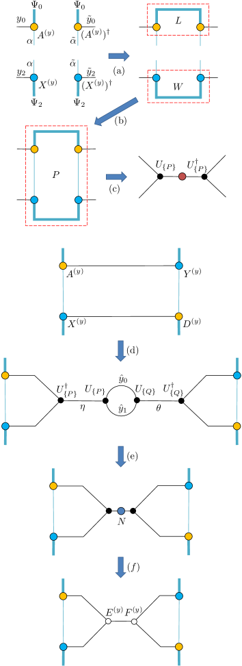
Before starting the method for $y$-axis, we reorder the bonds of $A$ and $X$ as

$$A^{(y)}_{\Psi_{0}y_{0}\alpha} =A_{\Omega_{0}x_{0}\alpha},$$ (32)

$$X^{(y)}_{\Psi_{2}\alpha y_{2}} =X_{\Omega_{2}\alpha x_{1}},$$ (33)

where the superscript $(y)$ represents the $y$-axis direction and $\Psi_{0}=(x_{0},z_{0},w_{0})$ and $\Psi_{2}=(x_{1},z_{2},w_{2})$. In step (a) of Fig. 9, the tensors and their conjugate tensors are contracted by summing up $\Psi$s as

$$L_{y_{0}\alpha\tilde{y}_{0}\tilde{\alpha}} =\sum_{\Psi_{0}}A^{(y)}_{\Psi_{0}y_{0}\alpha}(A^{(y)}_{\Psi_{0}\tilde{y}_{0}\tilde{\alpha}})^{*},$$ (34)

$$W_{y_{2}\alpha\tilde{y}_{2}\tilde{\alpha}} =\sum_{\Psi_{2}}X^{(y)}_{\Psi_{2}\alpha y_{2}}(X^{(y)}_{\Psi_{2}\tilde{\alpha}\tilde{y}_{2}})^{*},$$ (35)

In step (b) of Fig. 9, we contract $L$ and $W$ by summing up the bonds $\alpha$ and $\tilde{\alpha}$,

$$P_{y_{0}y_{2}\tilde{y}_{0}\tilde{y}_{2}} =\sum_{\alpha,\tilde{\alpha}}L_{y_{0}\alpha\tilde{y}_{0}\tilde{\alpha}}W_{y_{2}\alpha\tilde{y}_{2}\tilde{\alpha}}.$$ (36)

In step (c) of Fig. 9, we perform the SVD or the eigenvalue decomposition of $P$ and the truncation to retain $\chi$ largest singular values,

$$P_{y_{0}y_{2}\tilde{y}_{0}\tilde{y}_{2}} \simeq\sum_{\eta=1}^{\chi}U_{\{P\}y_{0}y_{2}\eta}S_{\{P\}\eta\eta}U^{*}_{\{P\}\tilde{y}_{0}\tilde{y}_{2}\eta},$$ (37)

where $U_{\{P\}}$ is an isometry made by the left singular vectors which corresponds to the $\chi$ largest singular values. We can also obtain $Q$ and $U_{\{Q\}}$ from $Y$ and $D$ in a similar way to $P$ and $U_{\{P\}}$. Then, in step (d) of Fig. 9, the isometries, $U^{\dagger}_{\{P\}},U_{\{P\}},U_{\{Q\}}$ and $U^{\dagger}_{\{Q\}}$, are inserted between $A^{(y)}X^{(y)}$ and $Y^{(y)}D^{(y)}$. To make $E^{(y)}$ and $F^{(y)}$ explicitly, $U_{\{P\}}$ and $U_{\{Q\}}$ are contracted as

$$N_{\eta\theta} =\sum_{\hat{y}_{0},\hat{y}_{1}}U_{\{P\}\hat{y}_{0}\hat{y}_{1}\eta}U_{\{Q\}\hat{y}_{0}\hat{y}_{1}\theta}.$$ (38)

in step (e) of Fig. 9. Next, in step (f) of Fig. 9, we carry out the SVD of $N$,

$$N_{\eta\theta} =\sum_{\kappa}U_{\{N\}\eta\kappa}S_{\{N\}\kappa\kappa}V_{\{N\}\theta\kappa},$$ (39)

and the contractions for making $E^{(y)}$ and $F^{(y)}$ as

$$E^{(y)}_{y_{0}y_{2}\kappa} =\sum_{\eta}\sqrt{S_{\{N\}\kappa\kappa}}U_{\{N\}\eta\kappa}U^{*}_{\{P\}\eta y_{0}y_{2}},$$ (40)

$$F^{(y)}_{y_{1}y_{3}\kappa} =\sum_{\theta}\sqrt{S_{\{N\}\kappa\kappa}}V_{\{N\}\theta\kappa}U^{*}_{\{Q\}\theta y_{1}y_{3}}.$$ (41)

We can use the same way to another direction, and $E$ and $F$ consist of the tensors of the directions other than the coarse-graining one such as

$$E =E^{(y)}\otimes E^{(z)}\otimes E^{(w)}$$ (42)

$$F =F^{(y)}\otimes F^{(z)}\otimes F^{(w)}.$$ (43)

To complete the making $E$ and $F$ step, it needs $4(d-1)$ times $O(\chi^{d+3})$ contractions, $2(d-1)$ times $O(\chi^{6})$ contractions and $2(d-1)$ times $O(\chi^{6})$ SVDs . Then, the bottleneck of this part is the $O(\chi^{d+3})$ contraction.

Appendix B Study of RSVD parameters

In this appendix, we study the parameters of the RSVD in the proposed algorithm and the original ATRG. The purpose of this study is to see how large the parameters of each algorithm should be taken to converge to the free energy density obtained by an ATRG algorithm which uses the truncation of the full SVD instead of the RSVD.

To investigate the convergence for the original ATRG, we use the Ising model on the $1024^{4}$ lattice and define the relative error of the free energy density as

$$\delta_{f}=\left|\frac{f_{n,\mathrm{RSVD}}-f_{\mathrm{SVD}}}{f_{\mathrm{SVD}}}\right|,$$ (44)

where $f_{\mathrm{SVD}}$ is the free enegy density obtained by ATRG which applies the truncation of the full SVD to $M$ and $f_{n,\mathrm{RSVD}}$ is the one using the original ATRG which applies the RSVD of $n$ oversamples and $\chi$ iterations to the matrix. In the case of the proposed algorithm, we can also define $\delta_{f}$ similarly. Note that if the number of the RSVD iterations is fixed to $\chi$, the computational cost of the swapping bond part in the original ATRG becomes $O(\chi^{10})$, and then the leading cost of the algorithm gets worse from $O(\chi^{9})$. On the other hand, the cost of the part in the proposed algorithm becomes $O(\chi^{8})$ and it is not the leading one in the whole algorithm (see Fig. 7). Figure 10 shows $\delta_{f}$ as the function of $n$ with $\chi=10,14$ and the temperatures are taken to be 6.65 and 6.68 ($t=6.65,6.68$).

Figure 10: The relative errors of the free energy densities of the Ising model on $1024^{4}$ lattice with the original ATRG and the proposed algorithm, where $\chi=10,14$, the temperatures are set to 6.65 and 6.68 ($t=6.65,6.68$), and then the number of the RSVD iterations is taken to be $\chi$. The oversampling parameter $n$ is changed from 1 to $2\chi$. We find that the results of the original ATRG and the proposed algorithm show similar behavior at $\chi=10$ and it is large enough to take $n\geq 20$ at $\chi=10,14$.

From Fig. 10, we can see that the results of the original ATRG and the proposed algorithm show similar behavior at $\chi=10$ and it is large enough to take $n\geq 20$ at $\chi=10,14$. Therefore, we use $\chi$ and $2\chi$ for the numbers of the RSVD iterations and oversamples respectively for the numerical results shown in Sec. IV. We believe that it is large enough for the RSVD to converge to the full SVD results when $\chi\geq 10$. Finally we remark that when degenerate singular values are truncated, the results of the RSVD may not converge to those of the full SVD even if the parameters are taken to be sufficiently large.

References

- (1) J. I. Cirac and F. Verstraete, J. Phys. A: Math. Theor. 42, 504004 (2009).
- (2) R. Orus, Ann. Phys., 349, 117, (2014).
- (3) S. R. White, Phys. Rev. Lett. 69, 2863, (1992).
- (4) S. R. White, Phys. Rev. B 48, 10345 (1993).
- (5) U. Schollwöck, Rev. Mod. Phys. 77, 259, (2005).
- (6) M. Fannes, B. Nachtergaele, and R. F. Werner, Commun. Math. Phys. 144, 443 (1992).
- (7) S. Östlund and S. Rommer, Phys. Rev. Lett. 75, 3537, (1995).
- (8) F. Verstraete and J. I. Cirac, arXiv (2004), cond-mat/0407066.
- (9) F. Verstraete, J.I. Cirac, and V. Murg, Adv. Phys. 57, 143 (2008).
- (10) J. Jordan, R. Orus, G. Vidal, F. Verstraete, and J. I. Cirac, Phys. Rev. Lett. 101, 250602 (2008).
- (11) M. Levin and C. P. Nave, Phys. Rev. Lett. 99, 120601 (2007).
- (12) Z. Y. Xie, J. Chen, M. P. Qin, J. W. Zhu, L. P. Yang, and T. Xiang, Phys. Rev. B 86, 045139 (2012).
- (13) Z. Y. Xie, H. C. Jiang, Q. N. Chen, Z. Y. Weng, and T. Xiang, Phys. Rev. Lett. 103, 160601, (2009).
- (14) Z. C. Gu and X. G. Wen, Phys. Rev. B 80, 155131, (2009).
- (15) G. Evenbly and G. Vidal, Phys. Rev. Lett. 115, 180405 (2015).
- (16) G. Evenbly, Phys. Rev. B 95, 045117 (2017).
- (17) S. Yang, Z. C. Gu, and X. G. Wen Phys. Rev. Lett. 118, 110504, (2017).
- (18) M. Bal, M. Marien, J. Haegeman, F. Verstraete, Phys. Rev. Lett. 118, 250602 (2017).
- (19) S. Morita, R. Igarashi, H.H. Zhao, and N. Kawashima, Phys. Rev. E. 97, 033310 (2018).
- (20) M. Hauru, C. Delcamp and S. Mizera, Phys. Rev. B 97, 045111 (2018).
- (21) K. Harada, Phys. Rev. B 97, 045124 (2018).
- (22) G. Evenbly, Phys. Rev. B 98, 085155 (2018).
- (23) Y. Nakamura, H. Oba, and S. Takeda, Phys. Rev. B 99, 155101 (2019).
- (24) S. Iino, S. Morita, and N. Kawashima, Phys. Rev. B 100, 035449 (2019).
- (25) D. Adachi, T. Okubo, and S. Todo, arXiv:1906.02007.
- (26) M. C. Bañuls, K. Cichy, K. Jansen and J. I. Cirac, JHEP 1311, 158 (2013).
- (27) S. Kühn, J. I. Cirac and M. C. Bañuls, JHEP 1507, 130 (2015).
- (28) M. C. Bañuls, K. Cichy, J. I. Cirac, K. Jansen and H. Saito, Phys. Rev. D 92, no. 3, 034519 (2015).
- (29) M. C. Bañuls, K. Cichy, K. Jansen and H. Saito, Phys. Rev. D 93, no. 9, 094512 (2016).
- (30) M. C. Bañuls, K. Cichy, J. I. Cirac, K. Jansen and S. Kühn, Phys. Rev. Lett. 118, no. 7, 071601 (2017).
- (31) M. C. Bañuls, K. Cichy, J. I. Cirac, K. Jansen and S. Kühn, Phys. Rev. X 7, no. 4, 041046 (2017).
- (32) Y. Shimizu, Mod. Phys. Lett. A 27, 1250035 (2012).
- (33) Y. Shimizu and Y. Kuramashi, Phys. Rev. D 90, no. 1, 014508 (2014).
- (34) Y. Shimizu and Y. Kuramashi, Phys. Rev. D 90, no. 7, 074503 (2014).
- (35) Y. Shimizu and Y. Kuramashi, Phys. Rev. D 97, no. 3, 034502 (2018).
- (36) A. Denbleyker, Y. Liu, Y. Meurice, M. P. Qin, T. Xiang, Z. Y. Xie, J. F. Yu and H. Zou, Phys. Rev. D 89, no. 1, 016008 (2014).
- (37) J. F. Yu, Z. Y. Xie, Y. Meurice, Y. Liu, A. Denbleyker, H. Zou, M. P. Qin and J. Chen,T. Xiang Phys. Rev. E 89, no. 1, 013308 (2014).
- (38) Y. Meurice, A. Bazavov, S. W. Tsai, J. Unmuth-Yockey, L. P. Yang and J. Zhang, PoS LATTICE 2016, 325 (2016).
- (39) S. Takeda and Y. Yoshimura, PTEP 2015, no. 4, 043B01 (2015).
- (40) H. Kawauchi and S. Takeda, Phys. Rev. D 93, no. 11, 114503 (2016).
- (41) R. Sakai, S. Takeda and Y. Yoshimura, PTEP 2017, no. 6, 063B07 (2017).
- (42) D. Kadoh, Y. Kuramashi, Y. Nakamura, R. Sakai, S. Takeda and Y. Yoshimura, JHEP 1803, 141 (2018).
- (43) W. E. Arnoldi, Quart. Appl. Math. 9, 17 (1951).
- (44) N. Halko, P. Martinsson and J. Tropp, SIAM Review 53, 217 (2011).
- (45) P. H. Lundow and K. Markström, Phys. Rev. E 80, 031104 (2009).
- (46) S. Akiyama, Y. Kuramashi, T. Yamashita, and Y. Yoshimura, arXiv:1906.06060.