Roychoudhury et al
*Satrajit Roychoudhury, New York NY.
Bayesian leveraging of historical control data for a clinical trial with time-to-event endpoint
Abstract
[Abstract]The recent 21st Century Cures Act propagates innovations to accelerate the discovery, development, and delivery of 21st century cures. It includes the broader application of Bayesian statistics and the use of evidence from clinical expertise. An example of the latter is the use of trial-external (or historical) data, which promises more efficient or ethical trial designs. We propose a Bayesian meta-analytic approach to leveraging historical data for time-to-event endpoints, which are common in oncology and cardiovascular diseases. The approach is based on a robust hierarchical model for piecewise exponential data. It allows for various degrees of between trial-heterogeneity and for leveraging individual as well as aggregate data. An ovarian carcinoma trial and a non-small-cell cancer trial illustrate methodological and practical aspects of leveraging historical data for the analysis and design of time-to-event trials.
keywords:
Historical data, hierarchical model, meta-analysis, time to event data, piecewise exponential model, prior distribution1 Introduction
Historical data often provide valuable information for the design of a new study. For example, sample size calculations depend on variability and effect sizes from previous trials. However, current practice usually ignores historical data in the analysis of a new trial. In recent years, however, leveraging historical data in the analysis of clinical trials has been encouraged by the European Medicines Evaluation Agency (EMEA) EMEA2014, the US Food and Drug Administration (FDA) including the Prescription Drug User Fee Act VI PDUFA6, and the 21st Century Cures Act USact21. Recent examples in various phases of drug and medical device development include French et al. French2012, Hueber et al. Hueber1693, and Campbell Campbell2017.
Leveraging historical data is appealing to practitioners and regulators for reasons of improved efficiency (smaller and therefore faster trials) and ethics (fewer patients assigned to a less effective treatment). Yet this may be challenging and requires care. First, identifying relevant historical data requires good judgment and collaboration by the various stakeholders of a clinical trial. A thorough review of the literature and other resources (e.g. registry data) in a specific disease (e.g., study population, definition of endpoint, data collection etc.) is important. This is ideally done using systematic reviews techniques (Egger et al. egg1995srh, Cochrane Collaboration CHMPmeta2001, Rietbergen et al. Rietbergen2011), and involving a third party or independent group may be useful.
Second, a principled statistical approach, which leverages the historical data while allowing for potential differences between historical and actual data, is needed. Various statistical methods have been proposed in this context: Pocock’s bias model Poc76, power priors (Ibrahim and Chen Ib00), commensurate priors (Hobbs et al. Hobbsetal2011), and meta-analytic-predictive priors (Spiegelhalter et al. Sp04, Neuenschwander et al. Neu10, Schmidli et al. Schmidli2014); for an overview, see Viele et al. Viele2014 and Lewis et al. Lewis2019. They are very similar and use hierarchical models that allow for different parameters in the historical and actual trial, which will imply discounting of the historical data when analyzing the new trial.
Here, we will be concerned with leveraging historical control data for time-to-event endpoints (e.g., time to disease progression, time to death). Such endpoints are the primary outcome in various therapeutic areas, including oncology and cardiovascular diseases. Among the various methods we will use the meta-analytic-predictive (MAP) approach. This is essentially a Bayesian random-effects meta-analysis of the historical data with the prediction of the parameter in the new trial. The basic model, which assumes exchangeable parameters for the new and the historical trials, can be extended in various ways. We will extend the MAP methodology for one-dimensional parameters to piecewise exponential (PWE) time-to-event data. To hedge against potential prior-data conflict, we propose an extension of the basic exchangeability assumption by adding a robust mixture component.
Although using historical data in clinical trials has gained increasing interest recently, applications in the time-to-event setting are sparse. A major challenge is the need of patient-level data for most of the statistical time-to-event approaches (Murray et al. Murray2014, Bertsche et al. Bertsche2017, and Hobbs et al. 2013 Hobbs2013). Our proposed methodology is applicable for both patient-level and summary data (e.g. Kaplan Meier curves), the latter often being available from publications.
The paper is structured as follows. In Section 2 we introduce the basic MAP methodology and extend it to time-to-event data. Two applications are discussed in Section 3, with emphasis on the analysis of trial data in the presence of historical data, and the design of a new trial leveraging historical data, respectively. Section 4 concludes with a discussion.
2 Methods
In this section we discuss a meta-analytic-predictive (MAP) approach to leveraging historical data for a time-to-event outcome. We consider the randomized setting, with a control and test treatment for which the use of historical data is confined to the control group. That is, while the prior distribution for the control (baseline) hazard will be informed by historical data, the prior for the treatment contrast (proportional hazards parameter) will be weakly informative.
2.1 The meta-analytic-predictive (MAP) prior distribution
The MAP approach uses the historical control data from trials to obtain the MAP prior distribution for the control parameter in the new study
| (1) |
The derivation of (1) is meta-analytic, using a hierarchical model with trial-specific parameters The simplest hierarchical model assumes exchangeable parameters across trials, which is usually represented as
| (2) |
While (2) allows for biases, they are assumed non-systematic. If needed, the basic model can be extended by replacing by to allow for systematic biases explained by covariates trial-specific covariates .
2.2 A hierarchical model for piecewise exponential time-to-event data
We assume piecewise exponential data and the time axis partitioned into intervals,
| (3) |
For each historical trial and time interval, there are control patients at risk (with a corresponding total exposure time ), of which experience an event. For each interval, the data model is Poisson
| (4) |
where is the hazard in interval of trial . Of interest is the prior for the control hazards in the new trial. The similarity of the new and the historical trials is captured in a parameter model. The simplest model assumes normally distributed log-hazard parameters ,
| (5) |
For the across-trial mean parameters , different implementations are possible. First, ignoring the time structure, the parameters may be assumed unrelated, with independent prior distributions
| (6) |
Second, the time structure of may be modelled using, for example, a multivariate normal distribution with a structured covariance matrix (e.g. AR(1)), or a dynamic linear model
| (7) | |||||
| (8) |
The latter will be used in the applications of Section 3, which gives more details for the prior distributions.
Finally, prior distribution for the across-trial standard deviations on the log-hazard scale are required. We will use half-normal priors
| (9) |
with scale parameter representing anticipated heterogeneity. A weakly-informative half-Normal prior with =0.5 puts approximately 5% probability for values of greater than 1. This allows small to large between trial heterogeneity. As for the mean parameters , rather than assuming unrelated parameters, a multivariate normal distribution or dynamic linear model could be used for the parameters.
From the above data model, parameter model, and prior distributions, the MAP prior for the vector of log-hazards in control group then follows as the conditional distribution of given historical data,
| (10) |
where and denote the number of events and exposure times across all historical trials and time intervals. The MAP prior can be obtained via MCMC. WinBUGS/JAGS code is given in the Appendix B.
2.3 Prior effective number of events
When desiging a new trial, knowing the amount of information introduced by the MAP prior is useful. It is sometimes expressed as the prior effective sample size (ESS), or, in the time-to-event setting, the effective number of events (ENE). Various methods have been suggested (Malec Malec2001, Morita et al. Morita2008, Neuenschwander et al. Neu10, Pennello and Thompson Pennello2008). They compare the information of the prior (variance or precision) to the one from one observation (or event). While conceptually similar, they can lead to suprisingly different ESS or ENE.
We will use an improvement, the expected local-information-ratio as introduced by Neuenschwander et al. Neuenschwander2019. It is defined as the expected (under the prior) ratio of prior information to Fisher information
| (11) |
where and .
It can be shown that, like the other methods, fulfills the necessary condition of being consistent with the well-known ESS for conjugate one-parameter exponential families. Unlike previous methods, however, it also fulfills a basic predictive criterion. That is, for a sample of size , the expected posterior ESS (under the prior distribution) is the sum of the prior ESS and .
For the piecewise exponential model with log-hazard parameters in the new trial, the Fisher information for one event is . Since the MAP priors for the log-hazard parameters are available only as an MCMC sample, approximations for will be needed. Mixtures of standard distributions are convenient and can approximate these distributions with any degree of accuracy (Dalal and Hall dallal1983, Diaconis and Ylvisaker dia1984qpo). Fitting mixture distributions can be done by various procedures (e.g., SAS SASref, R package RBesT web2019rbest,Weberetal2019). Finally, after having obtained the effective number of events for each log-hazard parameter, the total effective number of events of the MAP prior follows as .
2.4 Analysis of the data in the new trial
We now turn to the analysis of the new, randomized trial, where the control treatment will be compared to a test treatment . For the piecewise exponential model, the control and treatment data in interval follow Poisson distributions
| (12) |
where are the control hazards, and is the Cox proportional hazards parameter. Prior information for the control log-hazards are given by the MAP prior (10), whereas the prior for will usually be weakly-informative.
When leveraging historical data, the analysis for the new trial can be done in two ways.
-
•
Following the MAP approach, one would combine the MAP prior (10) from historical controls with the likelihood of the new data (12). This is complicated because the MAP prior for the control log-hazards is not known analytically but only available as an MCMC sample. Approximations of the MAP prior could be used; for example, by matching a multivariate normal distribution with the same means, standard deviations, and correlations; or, mixture approximations to the MAP priors could be used. The latter would allow for accurate approximations but would also be technically more complex.
-
•
Alternatively, the meta-analytic-combined (MAC) approach can be used. It consists of the hierarchical analysis of all the data and has been shown to be equivalent (Schmidli et al. Schmidli2014) to the MAP approach. Importantly, it is computationally easier than the two-step MAP approach and is therefore used here. For applications and respective code, see Section 3 and the Appendix, respectively.
2.5 Robust meta-analyses
To address the possibility of prior-data conflict, Schmidli et al. Schmidli2014 proposed robust versions of MAP or MAC analyses. The idea builds on exending the standard parameter model (exchangeable parameters), allowing the control parameter in the new trial to be non-exchangeable with the historical parameters. The implementation uses a mixture distribution with weights and for exchangeability and non-exchangeablity, respectively.
This idea can be easily extended to the time-to-event setting as follows: for each interval the robust version assumes exchangeablity, , with probability and non-exchangeability with probability . For the latter, interval-specific prior distributions
| (13) |
are needed. To achieve good robustness, weakly-informative priors should be used (for example, approximate unit-information priors, i.e., for exponential data on the log-scale). Of note, even though the are fixed, the Bayesian calculus ensures dynamic updating. That is, the prior weights will be updated to posterior weights depending on the similarity of the new and historical data. Eventually on may be interested in extending this idea to all trials by introducing trial-specific mixture weights , , .
3 Application
We now discuss two applications of leveraging historical time-to-event data. The first illustrates the joint analysis of historical and new data with the meta-analytic-combined approach of Section 2.4, whereas the second emphasizes the design of a new trial in the presence of historical data.
3.1 Analysis with historical data
Voest et al. Voe89 and Fiocco et al. Fio09SiM investigated survival data from ten studies on patients with advanced epithelial ovarian carcinoma. For our purpose, we assume the last study in Table 1 as the study of interest and the data of the remaining nine studies as the historical data. Thus, we want to infer the survival curve of the last study while leveraging the data from the other studies. The Kaplan-Meier plots in Figure 1 show considerable heterogeneity across the nine historical trials (left panel), with median survivals ranging from 1 to 2.9 years.
Fiocco et al. Fio09SiM used the following 12 invervals (in years): [0-0.25], (0.25-0.50], (0.50-0.75], (0.75-1], (1-1.25], (1.25-1.50], (1.50-1.75], (1.75- 2.08], (2.08-2.50], (2.50-2.92], (2.92-3.33], and (3.33-4]. For the following meta-analytic analyses, the number of deaths and total exposure time per interval have been extracted from the published Kaplan-Meier plots using the Parmar et al. Parmar1998 approach: the total exposure time () for interval and trial is calculated as
Here, is the interval length, and , and are the number of patients at risk, dead, and censored, respectively. The data extraction assumes constant censoring rates for each interval and all deaths at mid-interval times. Table 1 summarizes the data for the 12 intervals in the ten studies.


| historical studies | ||||||||||
| interval | 1 | 2 | 3 | 4 | 5 | 6 | 7 | 8 | 9 | new study |
| (years) | ||||||||||
| 0.00-0.25 | 1/9.4 | 9/21.1 | 1/21.9 | 1/5.6 | 5/6.4 | 0/17.8 | 2/8.0 | 0/9.2 | 2/5.2 | 1/23.4 |
| 0.25-0.50 | 3/8.8 | 1/19.9 | 3/21.4 | 2/5.2 | 3/5.4 | 6/17.0 | 2/7.5 | 1/9.1 | 0/5.0 | 5/22.6 |
| 0.50-0.75 | 3/7.9 | 0/19.8 | 5/20.4 | 2/4.8 | 6/4.2 | 3/15.9 | 5/6.6 | 3/8.6 | 3/4.6 | 17/19.9 |
| 0.75-1.00 | 4/7.0 | 10/18.5 | 7/18.9 | 4/4.0 | 2/3.2 | 12/14.0 | 3/5.6 | 4/7.8 | 1/4.1 | 0/17.8 |
| 1.00-1.25 | 3/6.1 | 6/16.5 | 9/16.9 | 3/3.1 | 3/2.6 | 8/11.5 | 3/4.9 | 1/7.1 | 4/3.5 | 2/17.5 |
| 1.25-1.50 | 0/5.8 | 6/15.0 | 4/15.2 | 1/2.6 | 3/1.9 | 2/10.2 | 3/4.1 | 1/6.9 | 0/3.0 | 7/16.4 |
| 1.50-1.75 | 0/5.8 | 5/13.6 | 5/14.1 | 3/2.1 | 0/1.5 | 3/9.6 | 2/3.5 | 4/6.2 | 1/2.9 | 8/14.5 |
| 1.75-2.08 | 2/7.3 | 9/15.7 | 10/16.2 | 0/2.3 | 2/1.7 | 2/11.9 | 3/3.8 | 1/7.4 | 1/3.5 | 4/17.2 |
| 2.08-2.50 | 0/8.8 | 9/16.2 | 0/18.5 | 0/2.9 | 1/1.5 | 11/12.4 | 3/3.6 | 6/8.0 | 0/4.2 | 0/21.0 |
| 2.50-2.92 | 6/7.6 | 3/13.6 | 0/18.3 | 0/2.9 | 1/1.0 | 1/9.9 | 0/2.9 | 0/6.7 | 0/4.2 | 6/19.7 |
| 2.92-3.33 | 0/6.2 | 0/12.5 | 3/17.0 | 0/2.9 | 1/0.6 | 0/9.4 | 0/2.9 | 0/6.6 | 0/4.1 | 2/17.4 |
| 3.33-4.00 | 0/10.0 | 0/20.1 | 7/24.5 | 0/4.7 | 0/0.7 | 10/12.1 | 0/4.7 | 0/10.7 | 0/6.7 | 0/27.5 |
The prior information about the hazards in study ten is captured by the MAP prior. The respective prior for survival (median and 95%-intervals in right panel of Figure 1 ) shows a median of approximately 1.8 years (95% interval 0.9 to 2.7 years). The prior effective number of events (Section 2.3) is 58. Figure 1 shows the KM plots of nine historical data (left panel) and MAP prior (right panel). The KM curve of the tenth trial (thick solid line in the right panel) is also shown in Figure 1.
After having access to the data from trial 10, for illustration we will compare two MAC analyses and the stratified analysis:
-
(i)
EX: full exchangeability MAC analysis. This is model (5) with between-trial standard deviations following half-normal priors with scale 0.5, which cover small to large heterogeneity (95% interval (0.02,1.12)). For , unit-information prior , centered at log(0.31) (the overall estimated log-hazard for death), is used. priors are used for , .
-
(ii)
EXNEX: exchangeability-nonexchangeability MAC analysis. This is the robust analysis of Section 2.5, where for the tenth trials we assume weight 0.5 for exchangeability EX (5) and 0.5 for nonexchangeability (NEX) (13). For remaining nine trials full exchangeability is assumed (weight=1). For EX, the prior assumptions in (i) are used, whereas for NEX the priors are weakly-informative with means centered at the mean of the MAP prior and variances approximately worth one observation.
-
(iii)
STRAT: this is the analysis of the data from the tenth study only, ignoring the data from the historical trials. For , a non-informative prior is used. Similar to EX model, priors are used for , .
For the three analyses, the posterior summaries for yearly survival rates in trial ten are summarized in Table 2. The EX analysis provides smaller survival rates compared to the stratified analysis, and median survival is 2.01 years, considerably different from the observed median (2.7 years). On the other hand, the EXNEX analysis is more robust, with a median survival of 2.59 months.
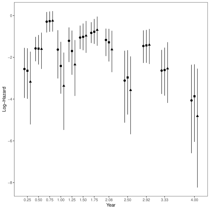
| EX | EXNEX | STRAT | |
|---|---|---|---|
| survival rate | |||
| 1 year | 0.72 (0.57, 0.86) | 0.74 (0.59, 0.86) | 0.75 (0.60, 0.87) |
| 2 year | 0.50 (0.31, 0.71) | 0.53 (0.31, 0.75) | 0.54 (0.32, 0.77) |
| 3 year | 0.43 (0.22, 0.67) | 0.45 (0.22, 0.71) | 0.47 (0.23, 0.73) |
| 4 year | 0.41 (0.19, 0.67) | 0.44 (0.20, 0.71) | 0.44 (0.20, 0.71) |
| median survival (years) | 2.24 (1.59, 3.19) | 2.62 (1.68, 5.05) | 7.90 (1.69, 39.86) |
3.2 Study design with historical data
The second application is concerned with the design of a randomized phase II trial for lung cancer with historical control data. As of 2018, lung cancer is the most common cause of cancer-related death in men and women, responsible for 1.76 million deaths annually worldwide ( WHO Cancer Factsheet 2018 WHOcancer2018).
The aim of the phase II proof-of-concept (POC) study was to compare a new treatment (T) against an active control treatment (C) for patients with locally advanced recurrent or metastatic lung cancer. The primary endpoint was progression-free survival (PFS), defined as the time from treatment assignment to disease progression or death from any cause. Superiority of the treatment T is typically established by a statistically significant log-rank test or an upper confidence limit of the Cox proportional hazard-ratio (HR) less than 1.
For the control treatment, the median PFS for this population is approximately five months. Assuming a 45% reduction in PFS for the new treatment, a 2:1 (T:C) randomization, an enrollment rate of 30 patients per month, a one-sided 2.5% level of significance and 90% power, the study would require 133 events (230 patients). Due to limited resources, however, it was decided to leverage historical data and enroll only 130 patients. For this modified design, the final analysis was planned after 110 events.
After an extensive search, seven historical studies with data for the active control were identified by the clinical team and disease area experts. Only Kaplan-Meier plots were available from the literature. Figure 3 shows the Kaplan-Meier plots as well as the number of events and exposure time for the following intervals (in days): (0-30], (30-60], (60-90], (90-120], (120-150], (150-180], (180-240], (240-300], and (300-360]. The data extraction from the Kaplan-Meier plots was done by the method of similar to Parmar et al. Parmar1998 ( for details see Appendix A). The Figure 3 shows the rather heterogeneous historical studies (medians vary between 3.5 months to 6 months) and the MAP prior (median= 4.88 months; 95% interval (1.6 months, 6.2 months)). The prior effective number of events (Section 2.3) is 36.

The frequentist operating characteristics (type-I error, power, bias, and root-mean-square error of the log-hazard ratio) of the design were assessed for exponential data, two scenarios for the HR (1 and 0.5), and various scenarios for the control median (3.5, 4.5, 5, 5.5, 6.5, and 7.5 months). Study success was defined by the Bayesian criterion or equivalently . For 2000 simulated trials, the above metrics were assessed for four models:
-
(i)
EX: full exchangeability MAC analysis. This is model (5) with between-trial standard deviations following half-normal priors with scale 0.5, which cover small to large heterogeneity (95% interval (0.02,1.12)). For , a unit-information prior , centered at log(0.00575) (the overall estimated log-hazard for death), was used. priors were used for , .
-
(ii)
EXNEX90: exchangeability-nonexchangeability MAC analysis. This is the robust analysis, with weights 0.9 for exchangeability EX (5) and 0.1 for nonexchangeability (NEX) (13). For EX, the prior assumptions in (i) were used, whereas for NEX the priors were assumed as weakly-informative with means centered at the mean of the MAP prior and variances equals 1 (worth one observation).
-
(iii)
EXNEX50: same as EXNEX90 but with 50-50 weights for exchangeability and nonexchangeability.
-
(iv)
STRAT: the analysis of the data from the new study only, ignoring the data from the historical trials and assuming priors for the log-hazards in each interval.
| scenarios | control | treatment | EX | EXNEX90 | EXNEX50 | STRAT |
|---|---|---|---|---|---|---|
| median | median | |||||
| HR=1 (type-I error) | ||||||
| 1 | 3.5 | 3.5 | 0.01 | 0.01 | 0.01 | 2.6 |
| 2 | 4.5 | 4.5 | 3.7 | 2.7 | 2.1 | 2.5 |
| 3 | 5.0 | 5.0 | 5.3 | 5.1 | 4.0 | 2.5 |
| 4 | 5.5 | 5.5 | 9.0 | 8.3 | 5.9 | 2.8 |
| 5 | 6.5 | 6.5 | 16.3 | 14.5 | 9.4 | 2.7 |
| 6 | 7.5 | 7.5 | 23.7 | 20.9 | 13.2 | 2.6 |
| HR=0.55 (power) | ||||||
| 7 | 3.5 | 6.4 | 91.7 | 90.9 | 88.6 | 85.2 |
| 8 | 4.5 | 8.2 | 97.3 | 96.9 | 94.5 | 84.9 |
| 9 | 5.0 | 9.1 | 97.0 | 96.8 | 96.1 | 84.6 |
| 10 | 5.5 | 10.0 | 98.9 | 98.7 | 97.1 | 85.0 |
| 11 | 6.5 | 11.8 | 99.3 | 99.2 | 98.0 | 84.8 |
| 12 | 7.5 | 13.6 | 99.7 | 99.5 | 98.5 | 84.5 |
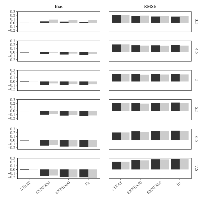
Table and Figure 4 summarize the operating characteristics for the four models.Table shows the type-I error and power for different scenarios. For the type-I error (HR=1), EX and EXNEX90 show fairly similar results. If the assumed control median is considerably smaller (3.5 months) than the one from the MAP prior ( months, Figure 3), the type-I error is much smaller than 2.5%. On the other hand, if the control median is much larger (6.5 or 7.5 months), the type-I error is larger than 10%. For the more robust EXNEX50 model, however, the type-I error is much less affected. Finally, for the Bayesian stratified analysis, the type-I error is close to the expected 2.5%. For power (HR=0.55), the analyses that leverage the historical data exhibit substantial gains compared to the stratified analyses, and power gains increase with increasing true control medians.
The bias on the log-HR scale (left panel of Figure 4) increases with increased leveraging (from stratified to fully exchangeable) and true control medians much smaller (3.5 months) or much larger (7.5 months) than suggested by the historical data (5 months). For the non-robust EX model, the bias is approximately –20% for the worst case scenario (true control median 6.5 months) but is generally much smaller for the robust analyses and true control medians closer to the expected 5 months.The root-mean-square error (on log-HR scale) (Figure 4) shows gain in efficiency in EX, EXNEX50, EXNEX90 when the new trial data are aligned with historical data.
4 Discussion
Clinical trials results are usually interpreted in the context of other relevant data. In addition to such informal considerations of historical data, or more generally co-data (Neuenschwander et al. Neuenschwander2016), we have considered leveraging historical data in the Bayesian analysis of a new clinical trial with a time-to-event endpoint. Historical control data are increasingly used in earlier stages of drug development. As these studies primarily inform company-internal decisions, the advantages are often considered to outweigh potential risks. In phase III clinical trials, however, historical controls are currently rare. Yet the regulatory environment is evolving in special areas such as rare diseases, pediatric populations, and non-inferiority trials (EMEA ema2006gct, ema2001gci, ema2006).
Leveraging historical control data has advantages. First, and most importantly, it allows randomizing fewer patients to the control group. This will shorten the duration of a clinical trial and hence lead to faster decisions. It will also decrease trial costs, as fewer patients will be needed. Second, if the control is ineffective (e.g., for placebo), historical data designs may also be more ethical because fewer patients receive the ineffective treatment (Berry berry2004).
The selection of historical data requires care and should follow recommendations for systematic reviews. This minimizes the risk of systematic biases, which can arise as a result of, for example, changes in standard of care over time, differences in inclusion/exclusion criteria, confounding environmental factors, or the evolution of diagnostic tools. The robust mixture approach proposed here mitigates some of these problems but cannot compensate for using biased data.
When analyzing the data of the new trial, a suitable model that allows for different degrees of similarity between historical and new data, is needed. Hierarchical models are the most obvious choice. For piecewise exponential time-to-event data, we have discussed a flexible model with interval-specific exchangeable hazard parameters and between-trial standard deviations. For few trials, which is typical for most settings, information on between-trial variability will usually be sparse. Yet valuable information may be available from similar disease settings, which may lead to more informative prior distributions for the between-trial standard deviations (Turner et al. tur2012peh, tur2015pdb). In the applications of Section 3, due to lack of additional information, we have used prior distributions that cover the range of small to large heterogeneity.
Widening the scope to real-world evidence, leveraging more but possibly less relevant data may be of interest. This will require adjustments to the methodology of Section 2 with regard to bias and heterogeneity. Having access to relevant predictors that explain anticipated biases will be key, and including these predictors (via meta-regression or propensity score methods) will be needed. Moreover, if historical data are of different quality, this may be accounted for by using different between-trial standard deviations. Further research will be needed to incorporate such extensions in the time-to-event setting.
Appendix A: Extraction of Data from Published Kaplan-Meier Plots
For the seven historical trials in Application 2 (NSCLC example),we could only get the Kaplan-Meier plots from the published articles. The data extraction (number of … ) was done using the following steps:
-
1.
The time axis is divided into intervals of 30 days up-to 180 days and 60 days afterwards. Based on historical data the maximum follow up time is restricted to 360 days.
-
2.
Probabilities of remaining progression-free at pre-specified time points are extracted using Engauge Digitizer Engauge2019, a freeware that converts an image to numbers.
-
3.
The number of patients at risk in a specific interval is calculated by multiplying the total number of patients with the probability of remaining progression-free at the beginning of the interval.
-
4.
The number of events (progression or death) within a time interval are approximated by using the probabilities of remaining progression-free in the current and next interval as follows;
where is the number of events and is the risk set for interval
-
5.
The exposure time for an interval is the interval length if the patient did not have an event or was not censored. Otherwise, the exposure of the patient is half the interval length. The total exposure time for an interval is the sum of the individual exposure times at the risk set.
Appendix B: WinBUGS Code for MAC Analysis
B.1 Main WinBUGS Code
##Required R packages

library(MASS)
library(coda)
library(R2WinBUGS)
library(survival)
library(RBesT)


##Main WinBUGS code

MAC.Surv.WB <- function()
{
# tau.study: Between study variation (Half normal)

Prior.tau.study.prec <- pow(Prior.tau.study[2],-2)

for ( t in 1:Nint) {

tau.study[t] ~ dnorm(Prior.tau.study[1], Prior.tau.study.prec) %_% I(0, )
tau.study.prec[t] <- pow(tau.study[t],-2)
}

#tau.time: correlation for piecewise exponential pieces (log-normal)

Prior.tau.time.prec <- pow(Prior.tau.time[2],-2)
tau.time ~ dlnorm(Prior.tau.time[1], Prior.tau.time.prec)
tau.time.prec <- pow(tau.time,-2)

# priors for regression parameter: h covariates

for (h in 1:Ncov) {
prior.beta.prec[h] <- pow(Prior.beta[2,h],-2)
beta[h,1] ~ dnorm(Prior.beta[1,h],prior.beta.prec[h])

}

###########################
#EXNEX structure of mu
###########################

#EX structure for mu is 1st order NDLM

mu.prec.ex <- pow(Prior.mu.mean.ex[2],-2)
mu.mean.ex ~ dnorm(Prior.mu.mean.ex[1],mu.prec.ex)


mu1.ex ~ dnorm(mu.mean.ex,tau.time.prec)
mu.ex[1] <- mu1.ex

prec.rho.ex <- pow(Prior.rho.ex[2],-2)

for(t in 2:Nint){

mu.dlm.ex[t] <- mu.ex[t-1] + rho.ex[t-1]

#variance of mu: discount factor X tau.time.prec

mu.time.prec.ex[t] <- tau.time.prec/w.ex

mu.ex[t] ~ dnorm(mu.dlm.ex[t], mu.time.prec.ex[t])

rho.ex[t-1] ~ dnorm(Prior.rho.ex[1], prec.rho.ex)

}

w.ex ~dunif(w1,w2)


#NEX structure for mu: unrelated structure
for( s in 1:Nstudies){
for(t in 1:Nint) {

prior.mu.prec.nex[s,t] <- pow(prior.mu.sd.nex[s,t],-2)
mu.nex[s,t] ~ dnorm(prior.mu.mean.nex[s,t],prior.mu.prec.nex[s,t])

}
}


# hazard-base: for each study (+ population mean + prediction) and time-interval t, no covariates
for ( s in 1:Nstudies) {

for ( t in 1:Nint) {
RE[s,t] ~ dnorm(0,tau.study.prec[t])

Z[s,t] ~ dbin(p.exch[s,t],1)

#For ex

log.hazard.base.ex[s,t] <- mu.ex[t] + step(Nstudies-1.5)*RE[s,t]

#For Nexch

log.hazard.base.nex[s,t] <- mu.nex[s,t]


log.hazard.base[s,t] <- Z[s,t]*log.hazard.base.ex[s,t]+(1-Z[s,t])*log.hazard.base.nex[s,t]


hazard.base[s,t] <- exp(log.hazard.base[s,t])
}
}


# likelihood: pick hazards according to study and time-invervals (int.low to int.high) for each
#observation j
# note: hazard is per unit time, not depending on length of interval t
for(j in 1:Nobs) {
for ( t in 1:Nint) {
# log.hazard for all time intervals
log(hazard.obs[j,t]) <- log.hazard.base[study[j],t] + inprod(X[j,1:Ncov],beta[1:Ncov,1])
}

#Poisson likelihood

alpha[j] <- (inprod(hazard.obs[j,int.low[j]:int.high[j]],int.length[int.low[j]:int.high[j]])
                                       /sum(int.length[int.low[j]:int.high[j]]))*exp.time[j]
n.events[j] ~ dpois(alpha[j])
n.events.pred[j] ~ dpois(alpha[j])

}

# outputs of interest (from covariate patterns in Xout)
for ( h in 1:Nout) {
for ( s in 1:Nstudies) {
# mean (index = Nstudies)
# surv: pattern x study x time
surv1[ h,s,1] <- 1
for ( t in 1:Nint) {
log(hazard[h,s,t]) <- log.hazard.base[s,t] + inprod(Xout[h,1:Ncov],beta[1:Ncov,1])
log.hazard[h,s,t] <- log(hazard.base[s,t])
surv1[h,s,t+1] <- surv1[h,s,t]*exp(-hazard[h,s,t]*int.length[t])
surv[h,s,t] <- surv1[h,s,t+1]
}
}
}

######### Prediction##########


for ( h in 1:Nout) {
for ( t in 1:Nint) {
hazard.pred[h,t] <- hazard[h,Nstudies,t]
log.hazard.pred[h,t] <- log(hazard[h,Nstudies,t]+pow(10,-6))
surv.pred[h,t] <- surv[h,Nstudies,t]
}
}


for (j in 1:Ncov) {
beta.ge.cutoffs[j] <- step(beta[j,1]-beta.cutoffs[j,1])
}

}
B.2 R wrapper function for running the main WinBUGS code
##Description of arguments of the function

#Nobs              =  Total number of data points
#study             =  Study indicator
#Nstudies          =  Number of studies
#Nint              =  Number of intervals
#Ncov              =  Number of covariates
#int.low, int.high =  Interval indicator
#int.length        =  Length of interval
#n.events          =  Number of events at each interval
#exp.time          =  Exposure time for each interval
#X                 =  Important covariates
#Prior.mu.mean.ex  =  Mean and standard deviation for normal priors for exchangeability for the first interval
#Prior.rho.ex      =  Mean and standard deviation for normal priors for random gradient of 1st order NDLM
#w1, w2            =  Upper and lower bound for uniform prior of the smoothing factor for 1st order NDLM model for exchangeability
#prior.mu.mean.nex =  Mean of normal prior for non-exchangeability
#prior.mu.sd.nex   =  Standard deviation for normal prior of non-exchangeability
#p.exch            =  Prior probability of exchangeability
#Prior.beta        =  Mean and standard deviation for normal priors of regression coefficients
#beta.cutoffs      =  Cut-off for treatment effect
#Prior.tau.study   =  Scale parameter of half-normal prior for between trial heterogeneity
#Prior.tau.time    =  Mean and standard deviation for log-normal prior for variance compoment of 1st order NDLM
#MAP.Prior         =  If TRUE: derives MAP prior
#pars              =  Parameters to keep in each MCMC run
#bugs.directory    =  Directory path where WinBUGS14.exe file resides
#R.seed            =  Seed to generate initial value in R (requires for reprducibility)
#bugs.seed         =  WinBUGS seed (requires for reprducibility)


MAC.Surv.anal <- function(Nobs  = NULL,
                          study             = NULL,
                          Nstudies          = NULL,
                          Nint              = NULL,
                          Ncov              = 1,
                          Nout              = 1,
                          int.low           = NULL,
                          int.high          = NULL,
                          int.length        = NULL,
                          n.events          = NULL,
                          exp.time          = NULL,
                          X                 = NULL,
                          Xout              = matrix(0,1,1),
                          Prior.mu.mean.ex  = NULL,
                          Prior.rho.ex      = NULL,
                          w1                = 0,
                          w2                = 1,
                          prior.mu.mean.nex = NULL,
                          prior.mu.sd.nex   = NULL,
                          p.exch            = NULL,
                          Prior.beta        = NULL,
                          beta.cutoffs      = NULL,
                          Prior.tau.study   = NULL,
                          Prior.tau.time    = NULL,
                          MAP.prior         = FALSE,
                          pars              = c("tau.study","log.hazard","mu.ex", "hazard"),
                          bugs.directory    = "C:/Users/roychs04/Documents/Folder/Software/WinBUGS14",
                          R.seed            = 10,
                          bugs.seed         = 12
                         )
{

set.seed(R.seed)

beta.cutoffs <- cbind(NULL,beta.cutoffs)

if(MAP.prior){Nstudies <- Nstudies+1}


#WinBUGS model

model <- MAC.Surv.WB


#Data for JAGS format

data     = list("Nstudies", "Nint", "Ncov", "Nobs", "Nout","study","int.low","int.high","int.length",
"n.events","exp.time",
"X","Xout",
"Prior.mu.mean.ex","Prior.rho.ex",
"prior.mu.mean.nex","prior.mu.sd.nex",
"p.exch","w1","w2",
"Prior.beta",
"beta.cutoffs",
"Prior.tau.study","Prior.tau.time"
)


#Initial values

hazard0 = (sum(n.events)+0.5)/sum(exp.time)


initsfun = function(i)
list(
mu1.ex = rnorm(1,log(hazard0),0.25),
tau.study = rgamma(12,1,1),
tau.time  = rgamma(1,1,1),
mu.mean.ex = rnorm(1,log(hazard0),0.1),
rho.ex = rnorm(Nint-1,0,0.05),
w.ex = runif(1,0,1),
beta=cbind(NULL,rnorm(Ncov,0,1))
)

inits <- lapply(rep(1,3),initsfun)


#WinBUGS run

fit = bugs(
data=data,
inits=inits,
par=pars,
model=model,
n.chains=3,n.burnin=8000,n.iter=16000,n.thin=1,
bugs.directory= bugs.directory,
bugs.seed= bugs.seed,
DIC= TRUE,
debug= FALSE
)

fit$sims.matrix = NULL
fit$sims.array = NULL


#WinBUGS summary

summary <- fit$summary
R2WB <- fit

output <- list(summary=summary,R2WB =R2WB)

return(output)

}
B.3 FIOCCO Analysis
##FIOCCO data set


FIOCCO.n.events <- c(1,  3,  3,  4,  3,  0,  0,  2,  0,  6,  0,  0,  9,  1,  0, 10,  6,  6,  5,  9,
                     9,  3,  0,  0,  1,  3,  5,  7,  9,  4,  5, 10,  0,  0,  3,  7,  1,  2,  2,  4,
                     3,  1,  3,  0,  0,  0,  0,  0,  5,  3,  6,  2,  3,  3,  0,  2,  1,  1,  1,  0,
                     0,  6,  3, 12,  8,  2, 3,  2, 11,  1,  0, 10,  2,  2,  5,  3,  3,  3,  2,  3,
                     3,  0,  0,  0,  0,  1,  3,  4, 1,  1,  4,  1,  6,  0,  0,  0,  2,  0,  3,  1,
                     4,  0,  1,  1,  0,  0,  0,  0,  1,  5, 17, 0,  2,  7,  8,  4,  0,  6,  2,  0)

FIOCCO.exp.time <- c(  9.4,  8.8,  7.9,  7.0,  6.1,  5.8,  5.8,  7.3,  8.8,  7.6,  6.2, 10.0, 21.1,
                      19.9, 19.8, 18.5, 16.5, 15.0, 13.6, 15.7, 16.2, 13.6, 12.5, 20.1, 21.9, 21.4,
                      20.4, 18.9, 16.9, 15.2, 14.1, 16.2, 18.5, 18.3, 17.0, 24.5,  5.6,  5.2,  4.8,
                       4.0,  3.1,  2.6,  2.1,  2.3,  2.9,   2.9,  2.9,  4.7,  6.4,  5.4,  4.2,  3.2,
                        2.6,  1.9,  1.5,  1.7, 1.5,  1.0,  0.6,  0.7, 17.8, 17.0, 15.9, 14.0, 11.5,
                      10.2,  9.6, 11.9, 12.4,  9.9,  9.4, 12.1,  8.0,  7.5,  6.6,  5.6,  4.9,  4.1,
                       3.5,  3.8,  3.6,  2.9,  2.9,  4.7,  9.2,  9.1,  8.6,  7.8,  7.1,  6.9,  6.2,
                       7.4,  8.0,  6.7,  6.6, 10.7,  5.2,  5.0,  4.6,  4.1,  3.5,  3.0,  2.9,  3.5,
                       4.2,  4.2,  4.1,  6.7, 23.4, 22.6, 19.9, 17.8, 17.5, 16.4, 14.5, 17.2, 21.0,
                      19.7, 17.4, 27.5)
B.3.1 Derivation of MAP Prior using First 9 Studies
FIOCCO.MAP.Prior <- MAC.Surv.anal(Nobs              = 108,
                                  study             = sort(rep(1:9,12)),
                                  Nstudies          = 9,
                                  Nint              = 12,
                                  Ncov              = 1,
                                  Nout              = 1,
                                  int.low           = rep(1:12,9),
                                  int.high          = rep(1:12,9),
                                  int.length        = c(0.25, 0.25, 0.25, 0.25, 0.25, 0.25, 0.25,
                                                        0.33, 0.42, 0.42, 0.41, 0.67),
                                  n.events          = FIOCCO.n.events[1:108],
                                  exp.time          = FIOCCO.exp.time[1:108],
                                  X                 = matrix(0,108,1),
                                  Prior.mu.mean.ex  = c(0, 10),
                                  Prior.rho.ex      = c(0,10),
                                  prior.mu.mean.nex = matrix(rep(0,108), nrow=9, ncol=12),
                                  prior.mu.sd.nex   = matrix(rep(1,108), nrow=9, ncol=12),
                                  p.exch            = matrix(rep(1,108), nrow=9),
                                  Prior.beta        = matrix(c(0,10), nrow=2) ,
                                  beta.cutoffs      = 0,
                                  Prior.tau.study   = c(0, 0.5),
                                  Prior.tau.time    = c(-1.386294, 0.707293),
                                  MAP.prior         = TRUE,
                                  pars              = c("tau.study","log.hazard.pred"),
                                  R.seed            = 10,
                                  bugs.seed         = 12
)

print(FIOCCO.MAP.Prior$summary)

#Calculation of ENE


FIOCCO.MAP.ess <- NULL

for(l in 1:12){

prior.ss.int <- FIOCCO.MAP.Prior$R2WB$sims.list$log.hazard.pred[,,l]
prior.ss.int.mix <- RBesT::automixfit(prior.ss.int, type="norm")


FIOCCO.MAP.ess[l] <- RBesT::ess(prior.ss.int.mix, sigma=1)


}


#Prior ESS (mixture)

FIOCCO.ESS.nevent <- sum(FIOCCO.MAP.ess)
B.3.1 MAC analysis of FIOCCO data
FIOCCO.anal.1 <- MAC.Surv.anal(Nobs              = 120,
                               study             = sort(rep(1:10,12)),
                               Nstudies          = 10,
                               Nint              = 12,
                               Ncov              = 1,
                               Nout              = 1,
                               int.low           = rep(1:12,10),
                               int.high          = rep(1:12,10),
                               int.length        = c(0.25, 0.25, 0.25, 0.25, 0.25, 0.25, 0.25,
                                                     0.33, 0.42, 0.42, 0.41, 0.67),
                               n.events          = FIOCCO.n.events,
                               exp.time          = FIOCCO.exp.time,
                               X                 = matrix(0,120,1),
                               Prior.mu.mean.ex  = c(-1.1711, 1),
                               Prior.rho.ex      = c(0,1),
                               prior.mu.mean.nex = matrix(rep(0,120), nrow=10, ncol=12),
                               prior.mu.sd.nex   = matrix(rep(1,120), nrow=10, ncol=12),
                               p.exch            = matrix(rep(1,120), nrow=10),
                               Prior.beta        = matrix(c(0,10), nrow=2) ,
                               beta.cutoffs      = 0,
                               Prior.tau.study   = c(0, 0.5),
                               Prior.tau.time    = c(-1.386294, 0.707293),
                               R.seed            = 10,
                               bugs.seed         = 12
                               )

print(FIOCCO.anal.1$summary)
B.3.2 Robust MAC analysis of FIOCCO data
FIOCCO.anal.2 <- MAC.Surv.anal(Nobs              = 120,
                               study             = sort(rep(1:10,12)),
                               Nstudies          = 10,
                               Nint              = 12,
                               Ncov              = 1,
                               Nout              = 1,
                               int.low           = rep(1:12,10),
                               int.high          = rep(1:12,10),
                               int.length        = c(0.25, 0.25, 0.25, 0.25, 0.25, 0.25, 0.25, 0.33,
                                                     0.42, 0.42, 0.41, 0.67),
                               n.events          = FIOCCO.n.events,
                               exp.time          = FIOCCO.exp.time,
                               X                 = matrix(0,120,1),
                               Prior.mu.mean.ex  = c(-1.1711, 1),
                               Prior.rho.ex      = c(0,1),
                               prior.mu.mean.nex = matrix(rep(c(-1.8625303, -1.6057708, -1.1242566,
                                                                -0.5940037, -0.5921193, -1.2484085,
                                                                -1.0011891, -0.9291769, -1.3337843,
                                                                -2.1254918, -2.9740698, -2.7570149),
                                                                10),
                                                                nrow=10, byrow = T),
                              prior.mu.sd.nex   = matrix(rep(1,12*10), nrow=10, byrow=T),
                              p.exch            = rbind(matrix(rep(1,108), nrow=9), rep(0.5, 12)),
                              Prior.beta        = matrix(c(0,10), nrow=2) ,
                              beta.cutoffs      = 0,
                              Prior.tau.study   = c(0, 0.5),
                              Prior.tau.time    = c(-1.386294, 0.707293),
                              R.seed            = 10,
                              bugs.seed         = 12
                              )

print(FIOCCO.anal.2$summary)
References
- 1