Non-thermal emission from cosmic rays accelerated in Hii regions

Abstract

Context. Radio observations at metre-centimetre wavelengths shed light on the nature of the emission of Hii regions. Usually this category of objects is dominated by thermal radiation produced by ionised hydrogen, namely protons and electrons. However, a number of observational studies have revealed the existence of Hii regions with a mixture of thermal and non-thermal radiation. The latter represents a clue as to the presence of relativistic electrons. However, neither the interstellar cosmic-ray electron flux nor the flux of secondary electrons, produced by primary cosmic rays through ionisation processes, is high enough to explain the observed flux densities.

Aims. We investigate the possibility of accelerating local thermal electrons up to relativistic energies in Hii region shocks.

Methods. We assumed that relativistic electrons can be accelerated through the first-order Fermi acceleration mechanism and we estimated the emerging electron fluxes, the corresponding flux densities, and the spectral indexes.

Results. We find flux densities of the same order of magnitude of those observed. In particular, we applied our model to the ‘deep south’ (DS) region of Sagittarius B2 and we succeeded in reproducing the observed flux densities with an accuracy of less than 20% as well as the spectral indexes. The model also gives constraints on magnetic field strength ($0.3-4$ mG), density ($1-9\times 10^{4}$ cm^-3), and flow velocity in the shock reference frame ($33-50$ km s^-1) expected in DS.

Conclusions. We suggest a mechanism able to accelerate thermal electrons inside Hii regions through the first-order Fermi acceleration. The existence of a local source of relativistic electrons can explain the origin of both the observed non-thermal emission and the corresponding spectral indexes.

1 Introduction

Massive stars ($M\gtrsim 8\leavevmode\nobreak\ {\rm M}_{\odot}$) strongly affect the dynamics, the morphology, and the chemistry of their hosting molecular clouds and galaxies, especially during the first stages of formation till their death as supernovae. Their scarcity, short lives, and large distances make them difficult to observe, and also because they are deeply embedded in their parental cloud at least during about 15% of their lifetimes (Churchwell 2002). However, even during the embedded phase, massive stars announce their presence by expanding Hii regions. This class of objects is routinely observed at infrared and radio wavelengths; the dust close to the Hii region absorbs most of the radiation from the star, emitting in the mid- and far-infrared, while the cool dust farther from the star absorbs the infrared radiation, emitting at sub-millimetre wavelengths. At metre-centimetre wavelengths, the emission is dominated by the interaction of free electrons and protons within the ionised gas.

Multiwavelength studies of Hii regions represent the classic approach to gather information on their morphology (Wood & Churchwell 1989) and their evolutionary stage (Kurtz 2005; Sánchez-Monge et al. 2013a). Observations at metre-centimetre wavelengths allow us to compute the spectral energy distribution, $S_{\nu}\propto\nu^{\alpha}$, and discriminate between thermal ($-0.1<\alpha<2$) and non-thermal emission ($\alpha<-0.1$). While the former can have different origins, such as (non-)homogeneous Hii regions; ionised equatorial winds; photoevaporated disc winds; thermal radiojets; dense interstellar shock waves (see Sánchez-Monge et al. 2013b, and references therein), the latter only originates from young stars with active magnetospheres giving rise to gyro-synchrotron emission (e.g. Feigelson & Montmerle 1999); and from fast shocks in discs or jets (e.g. Reid et al. 1995; Shchekinov & Sobolev 2004; Sanna et al. 2019) by the first-order Fermi acceleration mechanism (e.g. Crusius-Watzel 1990; Padovani et al. 2015, 2016; Rodríguez-Kamenetzky et al. 2017). Rodriguez et al. (1993) showed that a negative spectral index could also be due to dust absorption, but this would require dust mass column densities larger than $10^{3}$ g cm^-2.

Hii regions are usually dominated by thermal emission (e.g. Wood & Churchwell 1989; Kurtz 2005; Sánchez-Monge et al. 2008, 2011; Hoare et al. 2012; Purcell et al. 2013; Wang et al. 2018; Yang et al. 2019). However, observations with sensitive facilities such as the Very Large Array (VLA) or the Giant Metrewave Radio Telescope (GMRT) have revealed the presence of non-thermal emission in a handful of objects. Non-thermal emission in Hii regions usually shows up as spots surrounded by thermal emission (e.g. Nandakumar et al. 2016; Veena et al. 2016), contiguous to thermal emission as in cometary Hii regions (e.g. Mücke et al. 2002), or sometimes it appears isolated (Meng et al. 2019). Non-thermal emission observed in Hii regions is the fingerprint of the presence of relativistic electrons, but they cannot have interstellar origin. In fact, the interstellar cosmic-ray electron flux based on the most recent Voyager 1 observations (Cummings et al. 2016) is too low to explain the observed flux density. The same conclusion holds for the flux of secondary electrons created through ionisation processes by interstellar cosmic rays (protons and electrons) whose flux is strongly attenuated since Hii regions are located in embedded parts of molecular clouds (Padovani et al. 2009, 2018; see also Sect. 2).

A possible solution to explain the origin of these relativistic electrons is through a local acceleration inside the Hii region itself. Several mechanisms can be responsible for particle acceleration, such as turbulent second-order Fermi acceleration (Prantzos et al. 2011), acceleration by shocked background turbulence (Giacalone & Jokipii 2007), non-relativistic shear flow acceleration (Rieger & Duffy 2006), and acceleration in magnetic reconnection sites (de Gouveia dal Pino & Lazarian 2005). In this paper we focus on the first-order Fermi acceleration mechanism, also known as diffusive shock acceleration, according to which charged particles gain energy while crossing a shock back and forth due to the presence of magnetic fluctuations around the shock. Thus, charges are extracted from the thermal pool, accelerate up to relativistic energies, and escape in the downstream medium (e.g. Drury 1983; Kirk 1994).

This paper is organised as follows. In Sect. 2 we describe the model for particle acceleration and we compute the expected flux of shock-accelerated electrons in Hii regions, in Sect. 3 we recall the basic equations to compute the synchrotron specific emissivity and the corresponding flux density expected in Hii regions, in Sect. 4 we use our model to explain the origin of non-thermal emission in Sagittarius B2, and in Sect. 5 we discuss the implications of our results and summarise our most important findings.

2 Model for thermal particle acceleration

In this section we recall the main equations to compute the timescales involved in particle acceleration at a shock surface, computing the maximum energies and the emerging fluxes of shock-accelerated protons and electrons. For a detailed review of the methods, see O’C Drury et al. 1996 and Padovani et al. 2015, 2016.

2.1 Timescales

Thermal protons have to be accelerated before $(i)$ they lose energy from collisions, $(ii)$ they diffuse towards the source, and $(iii)$ the shock disappears. The acceleration timescale, $t_{\rm acc}$, is given by

$$t_{\rm acc}=2.9(\gamma-1)\frac{r[1+r(k_{\rm d}/k_{\rm u})^{\sigma}]}{k_{\rm u}^{\sigma}(r-1)}U_{2}^{-2}B_{-5}^{-1}\leavevmode\nobreak\ \mathrm{yr}\,,$$ (1)

where $U_{2}$ and $B_{-5}$ are the upstream flow velocity in the shock reference frame in unit of 100 km s^-1 and the upstream magnetic field strength in unit of 10 $\mu$G, respectively. Furthermore, $k_{\rm u,d}$ is the upstream and downstream diffusion coefficient that is normalised to the Bohm coefficient

$$k_{\rm u}=\left(\frac{\kappa_{\rm u}}{\kappa_{\rm B}}\right)^{-\sigma}=\left(\frac{3eB}{\gamma\beta^{2}m_{p}c^{3}}\kappa_{\rm u}\right)^{-\sigma}$$ (2)

with $e$ the elementary charge, $\gamma$ the Lorentz factor, $\beta=\gamma^{-1}\sqrt{\gamma^{2}-1}$, $m_{p}$ the proton mass, and $c$ the light speed. For a perpendicular shock $k_{\rm u}=rk_{\rm d}$ and $\sigma=1$, while for a parallel shock $k_{\rm u}=k_{\rm d}$ and $\sigma=-1$. Here, $r$ is the shock compression ratio defined by

$$r=\frac{\left(\gamma_{\rm ad}+1\right)M_{s}^{2}}{\left(\gamma_{\rm ad}-1\right)M_{s}^{2}+2}\,,$$ (3)

where

$$M_{s}=\frac{U}{c_{s}}$$ (4)

is the sonic Mach number,

$$c_{\rm s}=9.1[\gamma_{\rm ad}(1+x)T_{4}]^{0.5}\leavevmode\nobreak\ \mathrm{km\leavevmode\nobreak\ s^{-1}}$$ (5)

is the sound speed, $x=n_{i}/(n_{n}+n_{i})$ is the ionisation fraction ($n_{i}$ and $n_{n}$ are the ion and neutral volume density, respectively), and $T_{4}$ is the upstream temperature in unit of $10^{4}$ K. In the following, the adiabatic index is set to $\gamma_{\rm ad}=5/3$. Also, we assume Bohm diffusion ($k_{\rm u}=1$) and the shock to be parallel. For the case of deviations from Bohm diffusion regime and perpendicular shocks, see Sect. 2.2.

The general equation for the collisional energy loss timescale is given by

$$t_{\rm loss}=10\frac{\gamma-1}{\beta}n_{6}^{-1}L_{-16}\leavevmode\nobreak\ \rm{yr}\ ,$$ (6)

where $n_{6}$ is the volume density in unit of $10^{6}$ cm^-3 and $L_{-16}$ is the energy loss function in unit of $10^{-16}$ eV cm² (see Sect. 3 and Fig. 1 in Padovani et al. 2018). We can evaluate the mean loss timescale by averaging it over the particle’s up- and downstream residence times (Parizot et al. 2006)

$$\langle t_{\rm loss}\rangle=\left(\frac{t_{\rm loss,u}^{-1}+rt_{\rm loss,d}^{-1}}{1+r}\right)^{-1}\ .$$ (7)

The up- and downstream loss timescales differ in the density (downstream is a factor $r$ higher) and in the Coulomb component of the energy loss function, which depends on temperature (Mannheim & Schlickeiser 1994).

The upstream diffusion timescale, $t_{\rm diff,u}$, is obtained by assuming that the diffusion length in the upstream medium has to be a fraction $\epsilon<1$ of the distance between the central source and the shock, $R$, which is $\kappa_{\rm u}/U=\epsilon R$. The corresponding timescale is given by

$$t_{\rm diff,u}=22.9\epsilon\frac{k_{\rm u}^{\sigma}}{\gamma\beta^{2}}B_{-5}R_{2}^{2}\leavevmode\nobreak\ \mathrm{yr}\,,$$ (8)

where $R_{2}$ is the shock radius in unit of 100 AU. In the following we assume $\epsilon=0.1$. Since we modelled the particle acceleration in a Hii region, there is no further condition on the downstream escape timescale such as in protostellar jet shocks (see Sect. 2.5 in Padovani et al. 2016).

The determination of the age of an Hii region is not straightforward and it can be estimated in the following different ways: through ‘chemical clocks’ (e.g. Treviño-Morales et al. 2014), statistics (e.g. Wood & Churchwell 1989), and simulations (e.g. Peters et al. 2010a). All these methods give a lifetime of the order of $\approx 10^{4}$–$10^{6}$ yr. Here, we computed the dynamical timescale of an Hii region, $t_{\rm dyn}$, as a function of the shock radius and velocity,

$$t_{\rm dyn}=4.7R_{2}U_{2}^{-1}\leavevmode\nobreak\ \mathrm{yr}\,.$$ (9)

2.2 Non-Bohm diffusion regimes and perpendicular shocks

The upstream diffusion coefficient can be written as a function of the magnetic field strength and its turbulent component $\delta B$ (Drury 1983)

$$k_{\rm u}=\left(\frac{\kappa_{\rm u}}{\kappa_{\rm B}}\right)^{-\sigma}=\left(\frac{B}{\delta B}\right)^{2}\,.$$ (10)

The hypothesis of the Bohm diffusion regime implies $\delta B=B$, namely the magnetic fluctuations that determine the pitch angle scattering are large and particle acceleration is effective and works at its maximum degree. In the case of parallel shocks, deviations from the Bohm regime ($k_{\rm u}>1$) correspond to a reduction of $\delta B$, resulting in a lower acceleration efficiency and a decrease of the maximum energy reached, $E_{\rm max}$. Besides, the acceleration timescale increases since $t_{\rm acc}\propto k_{\rm u}$ (Eq. 1) and the parameter space where particle acceleration is efficient is reduced because of Coulomb losses (see Sect. 2.3.1 and Fig. 1 for more details).

For perpendicular shocks, the acceleration timescale decreases by a factor $(r+1)/2$ with respect to the parallel case and this results in a slight increase of $E_{\rm max}$. However, in the case of perpendicular transport, $E_{\rm max}$ is reduced by magnetic field line wandering (Kirk et al. 1996) and $k_{\rm u}$ is limited by requiring that particles have to be scattered in the time required to drift through the shock in order to avoid any anisotropy in the distribution of the accelerated particles (Jokipii 1987). For further details on perpendicular shocks and the non-Bohm regime, see Sect. 5.4.1 in Padovani et al. (2016).

2.3 Maximum energy and emerging flux at the shock surface

In the following subsections we describe how the maximum energy and the shock-accelerated particle flux is obtained for thermal protons (Sect. 2.3.1) and electrons (Sect. 2.3.2).

2.3.1 Acceleration of thermal protons

In order to provide an efficient acceleration, the flow has to be supersonic and super-Alfvénic, namely

$$U>\max(c_{\rm s},c_{\rm A})\,,$$ (11)

where the Alfvén speed is given by

$$c_{\rm A}=2.2\times 10^{-2}n_{6}^{-0.5}B_{-5}\leavevmode\nobreak\ \mathrm{km\leavevmode\nobreak\ s^{-1}}\,.$$ (12)

If this condition is fulfilled, the maximum energy reached by a thermal proton, $E_{\rm max,p}$, imposes

$$t_{\rm acc}=\min(t_{\rm loss},t_{\rm diff,u},t_{\rm dyn})\,.$$ (13)

We note that we assume the medium to be completely ionised ($x=1$) as expected in Hii regions. In Appendix A we show that as soon as $x<1,$ the particle acceleration efficiency drops.

In order to emphasise which mechanisms determine $E_{\rm max,p}$, in Fig. 1, we show the timescales for $T=10^{4}$ K, $U=40$ km s^-1, $B=100\leavevmode\nobreak\ \mu$G, $R=10^{5}$ AU, and three different values of the volume density. For $n=5\times 10^{2}$ cm^-3, $E_{\rm max,p}$ is determined by the upstream diffusion, whilst $n=10^{4}$ cm^-3 is constrained by collisional losses at high energies because of pion production. The timescale for collisional losses is shorter at low energies because of Coulomb losses. For example, Coulomb losses reduce $t_{\rm loss}$ by a factor of about 2, 5, and 250 at 0.1 GeV, 0.1 MeV, and 1 keV, respectively. This causes a strong damping in the acceleration efficiency at high volume densities (see $n=2\times 10^{5}$ cm^-3 in Fig. 1, and Sect. 3.2).

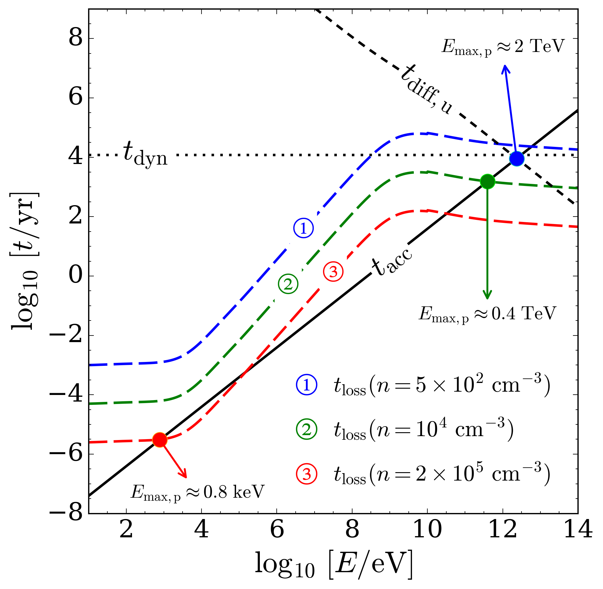
Figure 1: Acceleration timescale ($t_{\rm acc}$, solid black line), upstream diffusion timescale ($t_{\rm diff,u}$, short-dashed black line), and dynamical timescale ($t_{\rm dyn}$, dotted black line) versus proton energy for $T=10^{4}$ K, $U=40$ km s^-1, $B=100\leavevmode\nobreak\ \mu$G, and $R=10^{5}$ AU. The collisional loss timescale ($t_{\rm loss}$, long-dashed line plus colour-coding in the plot legend) depends on the density. The blue, green, and red dots show the value of the proton maximum energy for $n=5\times 10^{2}$ cm^-3, $10^{4}$ cm^-3, and $2\times 10^{5}$ cm^-3, respectively. We note that $E_{\rm max,p}$ is obtained by the intersection of $t_{\rm acc}$ with $t_{\rm diff,u}$ for $n=5\times 10^{2}$ cm^-3, while for the other two cases at higher $n$ by the intersection of $t_{\rm acc}$ with $t_{\rm loss}$.

The emerging flux at the shock surface is determined by the fraction of the ram pressure, $nm_{p}U^{2}$, which is transferred to the accelerated thermal particles, $\widetilde{P}$. Following Berezhko & Ellison (1999), $\widetilde{P}$ is proportional to the shock efficiency, $\eta$, which is the fraction of thermal plasma particles entering the acceleration process, and is given by

$$\widetilde{P}=\eta r\left(\frac{c}{U}\right)^{2}\widetilde{p}_{\rm inj}^{\,a}\left(\frac{1-\widetilde{p}_{\rm inj}^{\,b_{1}}}{2r-5}+\frac{\widetilde{p}_{\rm max}^{\,b_{2}}-1}{r-4}\right)\,,$$ (14)

where $a=3/(r-1)$, $b_{1}=(2r-5)/(r-1)$, $b_{2}=(r-4)/(r-1)$, and $\widetilde{p}_{k}=p_{k}/(m_{\rm p}c)$ is the normalised momentum. Subscripts $k={\rm inj,max}$ refer to the injection (or minimum) momentum of a particle able to cross the shock that enters the process of acceleration, and the maximum momentum reached by an accelerated particle, respectively. The injection momentum is related to the thermal particle momentum (Blasi et al. 2005) by

$$p_{\rm inj}=\lambda p_{\rm th}=\lambda m_{\rm p}c_{\rm s,d}\,,$$ (15)

where $c_{\rm s,d}$ is the sound speed in the downstream region, obtained by Eq. (5) for the downstream temperature. The parameter $\lambda$ is related to $\eta$ by

$$\eta=\frac{4}{3\sqrt{\pi}}(r-1)\lambda^{3}{\rm e}^{-\lambda^{2}}\,.$$ (16)

While in supernova remnants $\widetilde{P}$ is assumed to be of the order of 10%, shocks in Hii regions are slower and we expect $\widetilde{P}<$ 10% since pressure is smaller for slower shocks. At the same time $\widetilde{P}$ has to be high enough in order to explain the synchrotron radiation flux. In the following we used a typical value of $\widetilde{P}=1\%$, but we provide more accurate estimates for the Sgr B2(DS) case in Sect. 4. We recursively computed $\eta$ by coupling Eqs. (14) and (16) with the further condition $\lambda\gtrsim 2$, which guarantees that the accelerated particles are injected a few times $p_{\rm th}$.

Once $\widetilde{P}$ is fixed, $\eta$ depends only on the flow velocity in the shock reference frame and the temperature through $p_{\rm inj}$. The upper panel of Fig. 2 shows $\eta$ for $\widetilde{P}=1\%$ and typical values of $T$ and $U$ expected in Hii regions (see Sect. 3.2 and 4). The lower panel shows that the compression ratios are always lower than four and the strong shock approximation never holds.

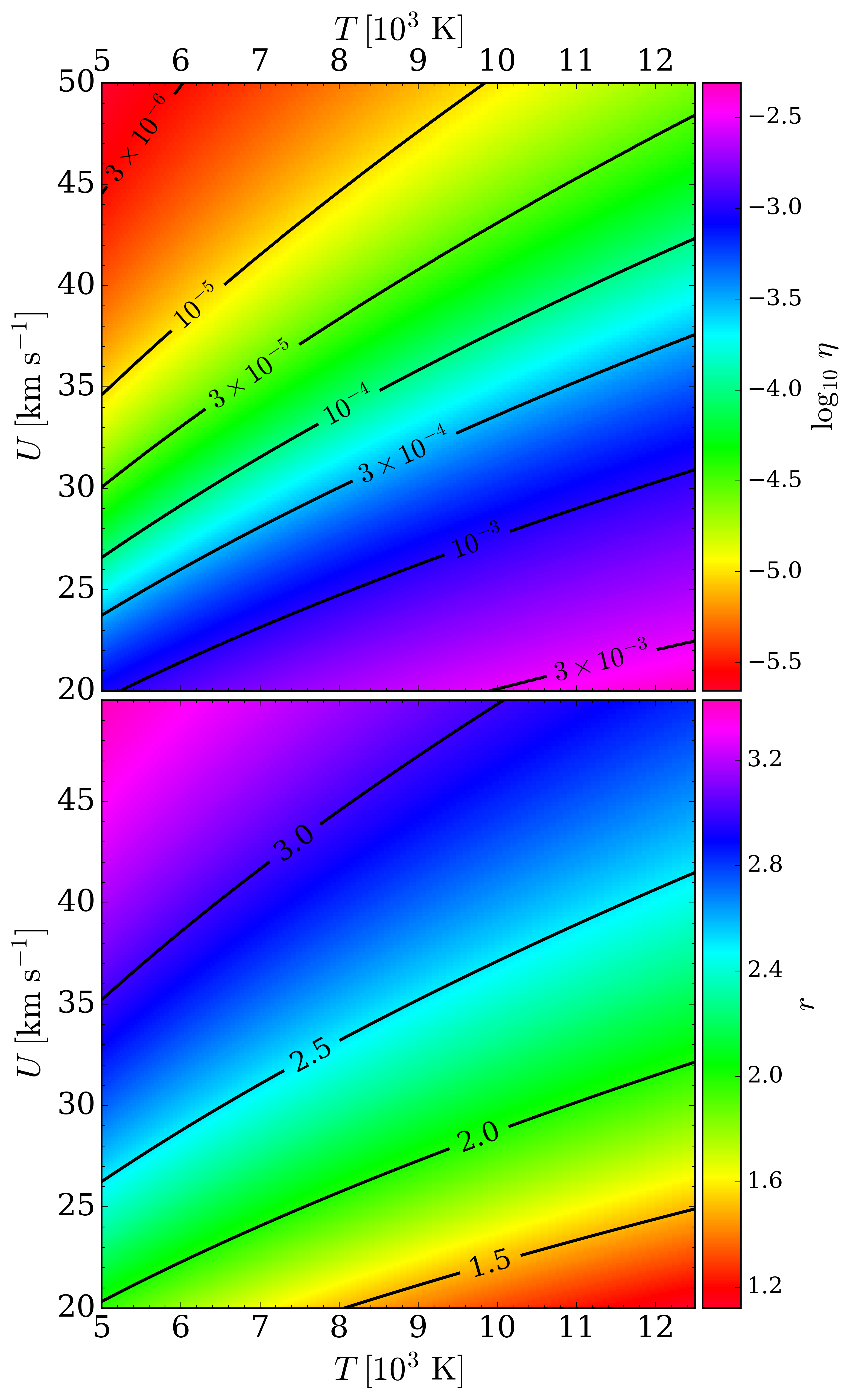
Figure 2: Shock efficiency, $\eta$ (upper panel), and compression ratio, $r$ (lower panel), for $\widetilde{P}=1\%$ as function of shock temperature and velocity. Solid black lines show iso-contours of values of $\eta$ and $r$.

The energy distribution per unit density (hereafter distribution) of shock-accelerated protons is given by

$$\mathscr{N}_{p}(E)=4\pi p^{2}f(p)\frac{\mathrm{d}p}{\mathrm{d}E}\,,$$ (17)

where $f(p)$ is the momentum distribution at the shock surface. In the test-particle regime, the latter is described by a power-law momentum function

$$f(p)=f_{0}\left(\frac{p}{p_{\rm inj}}\right)^{-q}\,,$$ (18)

with $q=3r/(r-1)$. The normalisation constant, $f_{0}$, is given by

$$f_{0}=\frac{3}{4\pi}\frac{n\widetilde{P}}{\mathscr{I}}\left(\frac{U}{c}\right)^{2}(m_{p}c)^{q-3}p_{\rm inj}^{-q}\,,$$ (19)

where

$${\mathscr{I}}=\int_{\widetilde{p}_{\rm inj}}^{\widetilde{p}_{\rm max}}\frac{p^{\,4-q}}{\sqrt{p^{\,2}+1}}\mathrm{d}p\,.$$ (20)

2.3.2 Acceleration of thermal electrons

The electron injection process in shock acceleration is poorly understood. As a guide, the model of Berezhko & Ksenofontov (2000) is used to estimate the distribution of shock-accelerated electrons, $\mathscr{N}_{e}$. Taking the same energy of the injected protons as that for electrons, namely $p_{\rm inj,e}=\sqrt{m_{e}/m_{p}}p_{\rm inj,p}$ ($m_{e}$ is the electron mass), at relativistic energies it holds

$$\frac{\mathscr{N}_{e}}{\mathscr{N}_{p}}=\left(\frac{m_{e}}{m_{p}}\right)^{(q-3)/2}\,.$$ (21)

The electron maximum energy, $E_{\rm max,e}$, is limited by synchrotron losses and it is obtained by equating the acceleration timescale (Eq. 1) to the synchrotron timescale, $t_{\rm syn}$, which is given by

$$t_{\rm syn}=2.7\times 10^{11}\frac{\gamma-1}{\gamma^{2}}B_{-5}^{-2}\leavevmode\nobreak\ \mathrm{yr}\,.$$ (22)

If $t_{\rm syn}>t_{\rm acc}$ at any energy, then we set $E_{\rm max,e}=E_{\rm max,p}$. Finally, we also accounted for the fact that at energies larger than $E^{*}$, where the condition $t_{\rm syn}(E^{*})<t_{\rm dyn}$ is fulfilled, the slope of the electron distribution, $s$, is modified from $\mathscr{N}_{e}(E)\propto E^{s}$ to $\mathscr{N}_{e}(E)\propto E^{s-1}$ (Blumenthal & Gould 1970).

Figure 3 shows an example of proton and electron fluxes emerging at the shock surface. Fluxes, namely the number of particles per unit energy, time, area, and solid angle, were computed from the corresponding distributions as

$$j_{k}=\frac{\beta_{k}c}{4\pi}\mathscr{N}_{k}\,,$$ (23)

where $k=p,e$. Here we consider $T=8\times 10^{3}$ K, $U=50$ km s^-1, $n=5\times 10^{4}$ cm^-3, $\widetilde{P}=1\%$, and $R=5\times 10^{4}$ AU. We set $B=1$ mG, high enough to shorten the synchrotron timescale so that the effect of the break in the slope of $\mathscr{N}_{e}$ occurs (in this case at $E^{*}\simeq 3$ GeV).

Most of the synchrotron radiation is emitted by electrons of energy

$$E_{\rm syn}\approx 1.47\left(\frac{\nu}{\rm GHz}\right)^{1/2}\left(\frac{B}{100\leavevmode\nobreak\ \mu{\rm G}}\right)^{-1/2}\leavevmode\nobreak\ \mathrm{GeV}\,,$$ (24)

see Longair (2011) and Padovani & Galli (2018). Figure 3 shows the electron energy range ($E_{\rm syn}\approx 0.1-5$ GeV) that mostly contributes to synchrotron radiation for $B=1$ mG and the three different frequency coverages of the Square Kilometre Array (SKA; $\nu=0.06-12.53$ GHz), GMRT ($\nu=0.16-1.42$ GHz), and VLA ($\nu=0.22-50$ GHz).

In this plot we also show the flux of secondary electrons (computed following Appendix B in Ivlev et al. 2015) generated by shock-accelerated protons and electrons through ionisation losses as soon as they propagate through a column density $N=10^{19}$ cm^-2, corresponding to a distance of about 13 AU at $n=4\times 10^{5}$ cm^-3. This secondary electron flux is much smaller than the shock-accelerated electron flux. For example, at 0.1, 1, and 5 GeV, the ratio between the fluxes of shock-accelerated electrons and secondary electrons is about 30, 220, and 2900, respectively. As a result, the contribution of secondary electrons to the synchrotron flux density is negligible as well as that of the interstellar electron flux obtained by the most recent Voyager 1 data release (Cummings et al. 2016). We note that Fig. 3 shows the unattenuated interstellar electron flux. This has to be considered as an upper limit since we expect strong attenuation effects at typical volume densities of Hii regions (see e.g. Padovani et al. 2009, 2018).

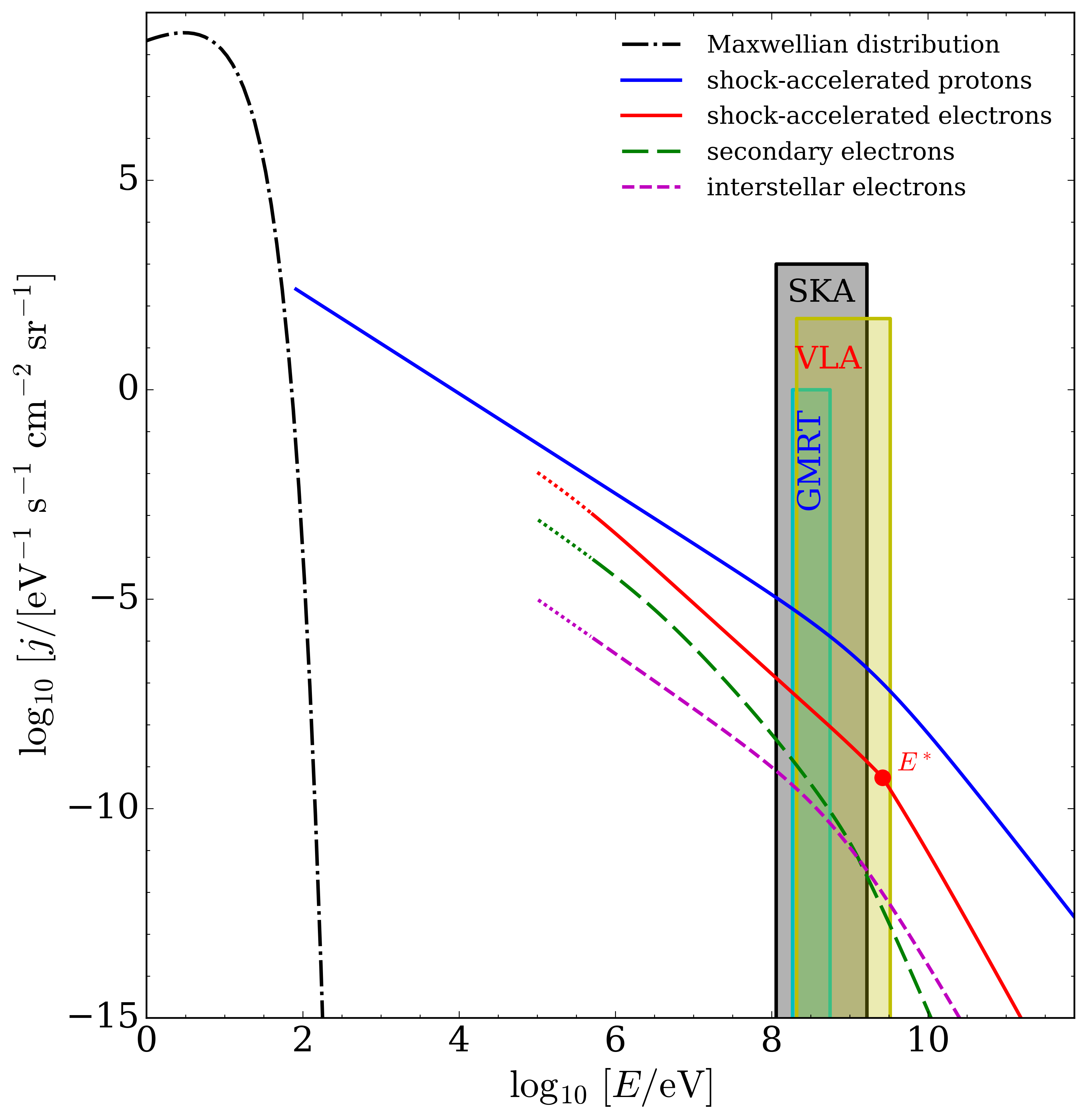
Figure 3: Shock-accelerated fluxes of protons (solid blue line) and electrons (solid red line), secondary electron flux (long-dashed green line), interstellar electron flux (short-dashed magenta line), and Maxwellian distribution of thermal protons (dash-dotted black line) as function of energy. The solid red circle shows the energy $E^{*}$ where synchrotron losses cause a break in the flux slope. The cyan-, black-, and yellow-shaded areas show the electron energy ranges mostly contributing to synchrotron emission for $B=1$ mG and frequency ranges of GMRT, SKA, and VLA telescopes, respectively (see Eq. 24). Dotted lines show the non-relativistic part of the electron fluxes.

3 Synchrotron emission in Hii regions

In this section we present the main equations for evaluating the synchrotron flux density and its spectral index (Sect. 3.1), which is followed by a description of the outcomes of the model applied to Hii regions (Sect. 3.2). Also, we comment on the linearly polarised nature of synchrotron radiation (Sect. 3.3).

3.1 Basic equations

The equations for computing flux density are listed in the following. For a detailed review, see Padovani & Galli (2018). The total power per unit frequency emitted by an electron of energy $E$ at frequency $\nu$ is given by

$$P_{\nu}^{\rm em}(E)=\frac{\sqrt{3}e^{3}}{m_{e}c^{2}}B_{\perp}F\left[\frac{\nu}{\nu_{c}(B_{\perp},E)}\right]$$ (25)

(see e.g. Longair 2011). Here, $B_{\perp}$ is the projection of the magnetic field on the plane perpendicular to the line of sight. The function $F$ is defined by

$$F(x)=x\int_{x}^{\infty}K_{5/3}(\xi)\mathrm{d}\xi\,,$$ (26)

where $K_{5/3}$ is the modified Bessel function of order 5/3 and

$$\nu_{c}(B_{\perp},E)=\frac{3eB_{\perp}}{4\pi m_{e}c}\left(\frac{E}{m_{e}c^{2}}\right)^{2}=4.19\left(\frac{B_{\perp}}{\rm G}\right)\left(\frac{E}{m_{e}c^{2}}\right)^{2}\leavevmode\nobreak\ {\rm MHz}$$ (27)

is the frequency at which $F$ reaches its maximum value. The synchrotron specific emissivity $\epsilon_{\nu}$ at frequency $\nu$, namely the power per unit solid angle and frequency produced within unit volume, is

$$\epsilon_{\nu}=\int_{m_{e}c^{2}}^{\infty}\frac{j_{e}(E)}{\beta_{e}(E)c}P_{\nu}^{\rm em}(E)\,\mathrm{d}E\,.$$ (28)

In principle, synchrotron self-absorption can take place if synchrotron radiation is sufficiently strong. As a consequence, the emitting electrons absorb synchrotron photons and the emission is quenched at low frequencies (see e.g. Rybicki & Lightman 1986). We computed the absorption coefficient per unit length as a function of the frequency, $\kappa_{\nu}$, given by

$$\kappa_{\nu}=-\frac{c^{2}}{2\nu^{2}}\int_{0}^{\infty}E^{2}\frac{\partial}{\partial E}\left[\frac{j_{e}(E)}{E^{2}\beta_{e}(E)c}\right]P_{\nu}^{\rm em}(E)\,\mathrm{d}E$$ (29)

and the optical depth $\tau_{\nu}=\kappa_{\nu}L$, where $L$ is the dimension of the emitting region. The size of Hii regions changes with time and it can be related as a first approximation to the evolutionary stage (see also Peters et al. 2010a, b). The earliest stages are classified as hypercompact, ultracompact, and compact Hii regions with sizes smaller than about 0.03 pc, 0.1 pc, and 0.5 pc, respectively (see e.g. Kurtz 2005). Even assuming the largest size for $L$ and frequencies as low as 60 MHz (the lowest SKA1-low frequency), we find the expected synchrotron emission to always be optically thin ($\tau_{\nu}\ll 1$). Thus, assuming a Gaussian beam profile, the synchrotron flux density at a frequency $\nu$, $S_{\nu}$, is given by

$$S_{\nu}=\frac{\pi}{4\ln 2}\epsilon_{\nu}\leavevmode\nobreak\ \theta_{b}^{2}\leavevmode\nobreak\ L\,,$$ (30)

where $\theta_{b}$ is the beam full width at half maximum.

3.2 Model results

The main parameters regulating the non-thermal emission in a Hii region are the temperature, the flow velocity in the shock reference frame, the magnetic field strength, the shock radius, and the dimension of the emitting region. In this section we computed the flux density assuming the following ranges which were obtained from observations and numerical simulations when possible: $5\times 10^{3}\leq T/{\rm K}\leq 1.2\times 10^{4}$, $20\leq U/({\rm km\leavevmode\nobreak\ s^{-1}})\leq 100$, $3\leq B/\mu{\rm G}\leq 10^{4}$, and $10^{2}\leq n/{\rm cm^{-3}}\leq 10^{5}$ (see e.g. Zuckerman et al. 1967; Heiles et al. 1981; Wink et al. 1983; Lockman 1989; Mehringer et al. 1993; Sewilo et al. 2004; Kurtz 2005; Harvey-Smith et al. 2011; Steggles et al. 2017). For simplicity, we assumed the shock radius to be equal to the dimension of the emitting region. Besides, since synchrotron emission has not been observed in hypercompact Hii regions so far, we let $L$ vary between 0.1 and 0.5 pc.

Figure 4 shows the results of our model for $T=7500$ K, $L=0.5$ pc, $\nu=300$ MHz, and $\theta_{b}=10\arcsec$. Each subplot shows the various quantities in the parameter space $(n,B)$. The three rows refer to three different values of the velocities ($U=30$, 40, and $50$ km s^-1) while the four columns display the maximum energy reached by the shock-accelerated protons, the mechanisms limiting $E_{\rm max,p}$, the flux density, and the spectral index, respectively. We note that at any density, for large magnetic field strengths, the condition required by Eq. (11) is not always fulfilled. In particular, the flow is sub-Alfvénic and no acceleration takes place (grey shaded area).

The iso-contours of $E_{\rm max,p}$ at 0.1 and 1 TeV in the first column exhibit a kink around $1-2\times 10^{3}$ cm^-3, which is due to the variation in the mechanism controlling $E_{\rm max,p}$. It is important to note that until the upstream diffusion constrains $E_{\rm max,p}$, the iso-contours are independent on density since $t_{\rm diff,u}\not\propto n$ (Eq. 8), but as soon as pion production losses take place, $E_{\rm max,p}$ decreases with increasing density since $t_{\rm loss}\propto n^{-1}$ (Eq. 6). As anticipated in Fig. 1, the low-energy ‘tail’ of the collisional energy loss timescale determined by Coulomb losses intersects the acceleration timescale at high densities, thus $E_{\rm max,p}$ suddenly drops to non-relativistic values and the acceleration process becomes ineffective.

Higher velocities increase the efficiency of shock acceleration and this affects the flux density magnitude, which increases with $U$, as shown in the third column. Since $t_{\rm acc}\propto U^{-2}$, the solution space shrinks for lower velocities, namely Coulomb losses become progressively more efficient, as seen in the plot of $S_{\nu}$ for $U=30$ km s^-1. The flux density increases with density until Coulomb losses prevail because $\mathscr{N}_{p}\propto f_{0}\propto n$ (Eqs. 17-19). In addition, $S_{\nu}$ increases with magnetic field strength until the flow becomes sub-Alfvénic since the synchrotron emissivity (Eq. 28) is proportional to $B^{\delta}$ with $s=1-2\delta$, where $s$ is the slope of the electron distribution (see Sect. 2.3.2 and Rybicki & Lightman 1986).

The rightmost column shows the spectral index, $\alpha$, of the flux density, $S_{\nu}\propto\nu^{\alpha}$ with $s=1+2\alpha$ (see e.g. Rybicki & Lightman 1986). The spectral index is independent of $n$, which only enters in the normalisation factor $f_{0}$ (Eq. 19), while it depends non-monotonically on $B$. In fact, for small magnetic field strength, $E_{\rm syn}$ (calculated from Eq. 24) is larger than the proton rest mass energy, where the proton (and electron) distribution slope is more negative than at non-relativistic energies. As $B$ increases, $E_{\rm syn}$ moves towards non-relativistic energies so that $s$ (and $\alpha$) increases. Finally, at very large $B$, we may enter the regime where the synchrotron timescale (Eq. 22) is smaller than the dynamical timescale (Eq. 9) and $\alpha$ decreases again because of the slope break at $E^{*}$ (see Sect. 2.3.2). The rightmost plot in the lower row also shows the relation between magnetic field strength and density, as given by Crutcher (2012), that falls inside the solution space of our model.

The dependence of $S_{\nu}$ on temperature in the range considered in this paper is negligible. In fact, temperature enters the Coulomb part of the loss timescale (see Mannheim & Schlickeiser 1994 and Eq. 6) so that the region of the parameter space $(n,B)$ dominated by Coulomb losses becomes slightly smaller for higher temperatures. The injection momentum is also a function of the (downstream) temperature through the downstream sound speed, $c_{\rm s,d}\propto\sqrt{T_{\rm d}}$ (Eq. 15). However, for increasing temperatures, $\eta$ increases (see Fig. 2) while $\lambda$ decreases (Eq. 16), and $p_{\rm inj}$ turns out to be only weakly dependent on temperature. For example, $p_{\rm inj}$ varies by less than 2% between $T=5\times 10^{3}$ K and $T=1.2\times 10^{4}$ K for $U=50$ km s^-1. Figure 4 has been obtained for $\nu=300$ MHz and $\theta_{b}=10\arcsec$. Since $S_{\nu}\propto\nu^{\alpha}$, we expect lower flux densities at higher frequencies since $\alpha$ is negative for non-thermal emission for a fixed beam size.

Figure 4: Model results for $T=7500$ K, $L=0.5$ pc, $\nu=300$ MHz, and $\theta_{b}=10\arcsec$ in parameter space $(n,B)$. Maximum energy of shock-accelerated protons ($E_{\rm max,p}$, first column) and its constraining timescales (second column), flux density ($S_{\nu}$, third column), and spectral index ($\alpha$, fourth column). The three rows show the above quantities at three different flow velocities in the shock reference frame ($U=30$, 40, and 50 km s^-1). Grey-shaded areas in each subplot show the region of the parameter space where the flow is sub-Alfvénic. Solid white lines in the first column show the iso-contours of $E_{\rm max,p}$ at 0.1 and 1 TeV. Solid black lines in each subplot (except for the bottom right plot where black has been replaced by light grey) show the iso-flux density between 1 and 100 mJy (from the bottom up). The relation between magnetic field strength and density by Crutcher (2012) together with its uncertainty is shown in the rightmost subplot of the lowest row by a solid magenta line surrounded by a shaded region.

To facilitate the application of our model to a generic Hii region, we developed a publicly available web-based application that allows the user to compute the flux density per beam squared and per size of the emitting region, $S_{\nu}/(\theta_{b}^{2}L)$, the spectral index, and the shock-accelerated electron flux for a given set of parameters (temperature, shock velocity, and observing frequency) in the parameter space ($n,B$).

3.3 Polarisation observations

Synchrotron emission is linearly polarised (see e.g. Longair 2011) and the fractional polarisation, $\Pi$, is related to the electron distribution slope and the spectral index by

$$\Pi=\frac{1-s}{7/3-s}=\frac{3-3\alpha}{5-3\alpha}\,.$$ (31)

For example, spectral indexes between $-1$ and $-0.2$ correspond to a fractional polarisation equal to 75% and 64%, respectively. As a result, polarisation observations could be very useful to confirm the non-thermal nature of this emission. These kind of observations would also be helpful in determining the type of shock and whether it is parallel or perpendicular. It is important to note that there would be consequences on the maximum energy reached by the accelerated particles (see Sect. 2.1). In addition, information on the magnetic field morphology and the shock type would allow us to refine the model and to describe the propagation of shock-accelerated electrons (and protons) along the magnetic field lines as soon as they leave the shock (see e.g. Padovani & Galli 2011; Padovani et al. 2013).

We note, however, that we assume Bohm diffusion, namely the turbulent component of the magnetic field is of the order of the magnetic field strength itself (see Sect. 2.2). As a consequence the magnetic field should be randomly oriented, at least downstream, resulting in no polarisation detection. In the case of non-Bohm diffusion, the magnetic field is more ordered and the detection of linear polarisation could be more likely. This could be the case for Sgr B2(DS) for which we estimated $k_{\rm u}$ of the order of 10 (see Sect. 4). However, a high electron density at the shock position could cause Faraday depolarisation of the synchrotron emission, which is stronger at lower frequencies.

4 Comparison with observations

There are some important caveats that we have to consider, both when attempting to model a synchrotron source as well as when interpreting observations. The flux density that we obtained from observations is the sum of the specific emissivity of each position along the line of sight convolved with the beam. In fact, the magnetic field strength and the locally accelerated electron flux, which determine the power per unit frequency (Eq. 25) and the emissivity (Eq. 28), are ‘local’ functions that namely depend on position. Besides, in Sect. 2.3.2 we show that the energy slope of shock-accelerated electrons is not constant. It becomes more negative above the proton rest mass energy and there can be a further steepening at energies larger than $E^{*}$ where the condition $t_{\rm syn}(E^{*})<t_{\rm dyn}$ is satisfied (see Fig. 3). For a given observing frequency, the energy of the electrons responsible for synchrotron emission depends on the magnetic field strength (Eq. 24), which is not constant along the line of sight. This means that we map different parts of the electron flux, and different slopes, as a function of the position, both along the line of sight and on the plane of the sky.

In our model we assume a constant value for $B$ and a unique energy distribution of shock-accelerated electrons. With only the knowledge of the volume density profile and the magnetic field topology, it would be possible to compute the attenuation of the electron flux, accounting for magnetic effects on particle propagation (following e.g. Padovani et al. 2009; Padovani & Galli 2011; Padovani et al. 2013, 2018). As a result, by comparing modelled and observed flux densities, we estimated an average value of quantities such as temperature, flow velocity in the shock reference frame, magnetic field strength, and volume density. For a proper modelling of the flux density, one should know both the density and the magnetic field strength profiles, as shown by Padovani & Galli (2018).

Another important point is the way in which we interpret the spectral index, $\alpha$. The value of $\alpha$ estimated from observations can be strongly dependent on the observed frequencies. For example, Veena et al. (2016) carried out GMRT observations at 325, 610, and 1372 MHz in the Hii region IRAS 17256-3631, finding non-thermal emission at two positions. The spectral indexes computed at lower frequency ($325-610$ MHz) is clearly non-thermal ($\alpha=-0.91$ and $-1.25$), but at higher frequency ($610-1372$ MHz) the thermal contribution dominates ($\alpha=-0.07$ and $0.09$). The benefit of the model presented in this paper is that $\alpha$ is computed as a local derivative of the flux density and this allows us to make predictions on its value at any frequency.

Meng et al. (2019) carried out VLA observations at $4-12$ GHz towards the Sagittarius B2 complex, finding a mixture of thermal and non-thermal emission in the ‘deep south’ region, hereafter Sgr B2(DS). This is possibly due to an expanding Hii region. This region has the shape of a shell with inner and outer radius $R_{\rm in}\simeq 0.36$ pc and $R_{\rm out}\simeq 0.72$ pc, respectively, to which corresponds an average size of the emitting region $L=(\pi/2)R_{\rm out}(1-R_{\rm in}^{2}/R_{\rm out}^{2})=0.85$ pc. Within this framework we applied the model described in Sect. 2 in order to explain the origin of the synchrotron emission. We assumed a parallel shock, a temperature of $8\times 10^{3}$ K (Mehringer et al. 1993; Meng et al. 2019), and the same beam size and frequency range of VLA observations, namely $\theta_{b}=4\arcsec$ and $\nu=4-12$ GHz, respectively. We also assumed $\widetilde{P}=5\%$ to explain the non-thermal flux densities observed in DS.

For each of the five positions where a negative spectral index was computed from observations (see Fig. 5 in Meng et al. 2019), we compiled a library of models varying flow velocities in the shock reference frame, densities, and magnetic field strengths in the range $20\leq U/({\rm km\leavevmode\nobreak\ s^{-1}})\leq 100$, $10^{3}\leq n/{\rm cm^{-3}}\leq 10^{5}$, and $0.1\leq B/{\rm mG}\leq 10$, respectively. We note that the velocity range considered is in agreement with what was obtained by simulations of cometary Hii regions of O and B stars driving strong stellar winds (Steggles et al. 2017). We performed a $\chi^{2}$ test identifying the best $U$, $n$, and $B$ values that reproduce the observed flux densities. At first we considered the Bohm diffusion regime ($k_{\rm u}=1$) then, using the values of $U$, $n$, and $B$ from the $\chi^{2}$ test, we recomputed the upstream diffusion coefficient following Pelletier et al. (2006)

$$k_{\rm u}=4\times 10^{-4}U_{2}^{-1}n_{6}^{-0.5}B_{-5}\widetilde{P}^{-1}\,,$$ (32)

and repeated the procedure till $k_{\rm u}$ converges. We found $k_{\rm u}$ to be of the order of ten for all five positions, which indicates a regime of non-Bohm diffusion.

The results of the $\chi^{2}$ minimisation are shown in Table 1, where the $1\sigma$ errors on $U$, $n$, and $B$ were estimated using the method of Lampton et al. (1976). The observed flux densities fall in the range $1-40$ mJy and they were reproduced by our model with an average accuracy of 5% for magnetic field strengths spanning between about 0.6 and 3 mG, densities between about 3 and $6\times 10^{4}$ cm^-3, and shock velocities between 35 and 45 km s^-1 (see Fig. 5). We noticed that our model allowed us to discard velocities lower than about 35 km s^-1, which cannot explain the observed flux densities since $t_{\rm acc}\propto U^{-2}$ and the particle acceleration process becomes rapidly inefficient for decreasing velocities (see Sect. 3.2). It is remarkable that the modelled spectral indexes, $\alpha_{\rm mod}$, which are obtained as a by-product of the $\chi^{2}$ minimisation, are also within the error bars of the observed spectral indexes $\alpha_{\rm obs}$ (see Table 1). It is interesting to note that in Meng et al. (2019), we applied the model to explain the non-thermal emission in the whole Sgr B2(DS) region with an average accuracy lower than 20%. We obtained the distributions of velocities, densities, and magnetic field strengths, which give information on the dynamics of DS. In fact, we found low velocities ($33\leq U/({\rm km\leavevmode\nobreak\ s^{-1}})\leq 40)$ towards north, where density and magnetic field strength are higher, and velocities in the range $40-50$ km s^-1 in the transverse east-west direction, where density and magnetic field strength are lower, as if the Hii region were expanding towards the direction of minimum resistance (see Meng et al. 2019 for details).

position	$U$	$n$	$B$	$\langle(S_{\nu,\rm obs}-S_{\nu,\rm mod})/S_{\nu,\rm obs}\rangle$	$\alpha_{\rm mod}$	$\alpha_{\rm obs}$
	[km s-1]	[$10^{4}$ cm-3]	[mG]	[%]
$a$	$44_{-0.4}^{+0.3}$	$3.50_{-0.10}^{+0.05}$	$1.44_{-0.11}^{+0.11}$	4.0	$-0.76$	$-0.76\pm 0.12$
$b$	$45_{-0.2}^{+0.2}$	$4.55_{-0.03}^{+0.03}$	$0.957_{-0.028}^{+0.031}$	1.1	$-0.58$	$-0.61\pm 0.09$
$c$	$34_{-0.2}^{+0.2}$	$5.92_{-0.54}^{+0.48}$	$3.26_{-0.09}^{+0.10}$	8.3	$-1.01$	$-1.24\pm 0.23$
$d$	$45_{-0.3}^{+0.6}$	$4.17_{-0.06}^{+0.10}$	$0.574_{-0.031}^{+0.026}$	6.0	$-0.50$	$-0.38\pm 0.13$
$e$	$43_{-1.1}^{+1.0}$	$2.47_{-0.19}^{+0.19}$	$0.864_{-0.010}^{+0.015}$	2.9	$-0.57$	$-0.58\pm 0.21$

Table 1: Results of the $\chi^{2}$ minimisation for the five positions observed in Sgr B2(DS), see Fig. 5 in Meng et al. (2019). Flow velocity in the shock reference frame, volume density, and magnetic field strength (columns 2 to 4), average difference in percent between the observed and the modelled flux density ($S_{\nu,\rm mod}$ and $S_{\nu,\rm obs}$; column 5), and modelled and observed spectral indexes ($\alpha_{\rm mod}$ and $\alpha_{\rm obs}$; columns 6 and 7).

Figure 5: Observed flux densities (magenta squares) and their best fits (dashed black lines) for five positions in DS as function of frequency (labelled $(a)$ to $(e)$; see Fig. 5 in Meng et al. 2019). Solid black lines show the model results (see Tab. 1 for a complete overview of the model parameters). Each subplot also displays the modelled and observed spectral indexes, $\alpha_{\rm mod}$ and $\alpha_{\rm obs}$, respectively.

Sgr B2(DS) is a special case where non-thermal emission is found all along the ionised bubble, especially in the inner part, which is expected to be closer to the shock and namely to the particle acceleration site. As a result, the application of the model is more straightforward with respect to Hii regions, such as those associated with IRAS 17160-3707 (Nandakumar et al. 2016) and IRAS 17256-3631 (Veena et al. 2016). Indeed, these latter sources show thermal emission with some localised spots of non-thermal emission. Additionally, proper modelling would require knowledge of the spatial variation of all the parameters including the flow velocity in the shock reference frame, density, and magnetic field strength. This goes beyond the scope of the present paper, but we presume that non-thermal emission spots in these IRAS sources could be explained by shock-accelerated electrons as in Sgr B2(DS).

5 Discussion and conclusions

We explored the possibility of thermal electrons accelerating up to relativistic energies in Hii regions through the first-order Fermi acceleration mechanism, assuming that shocks are located at the position where non-thermal emission is detected through radio observations. We computed the shock-accelerated electron flux and the corresponding flux density by assuming a completely ionised medium and by studying the parameter space for the following quantities: temperature ($5-12\times 10^{3}$ K), flow velocity in the shock reference frame ($20-100$ km s^-1), magnetic field strength ($3-10^{4}\leavevmode\nobreak\ \mu$G), and density ($10^{2}-10^{5}$ cm^-3).

We found that the modelled flux densities are of the same order of those observed and we concluded that non-thermal emission in Hii regions might be due to synchrotron radiation from locally accelerated electrons braked in a magnetic field. Assuming Bohm diffusion, this mechanism is efficient if $U>30$ km s^-1. These high velocities are of the same order of those obtained by numerical simulations of O and B stars generating Hii regions by powerful stellar winds. The acceleration efficiency is also quenched as soon as the medium is not completely ionised ($x<1$) because ions and neutrals are not coupled; even an ionisation degree of 95% strongly reduces the range of densities and magnetic field strengths corresponding to flux densities comparable to those observed.

We applied our model to Sgr B2(DS) in order to explain the observed flux densities and the spectral indexes (Meng et al. 2019). By means of a $\chi^{2}$ test, we found that flux densities in the frequency range $4-12$ GHz can be carefully reproduced by our model with an average accuracy lower than 20% by assuming a parallel shock, a completely ionised medium, a temperature of 8000 K, and for magnetic field strengths, densities, and velocities in the ranges $0.3-4$ mG, $1-9\times 10^{4}$ cm^-3, and $33-50$ km s^-1, respectively. It is worth noting that the modelled spectral indexes, which are a by-product of the $\chi^{2}$ test, fall within the errors of the spectral indexes computed from observations. Considering the relative simplicity of our model, this is a promising result, even if in principle one should model an Hii region accounting for the spatial variation of density, magnetic field strength, and velocity, for example.

The best model for Sgr B2(DS) is obtained for an upstream diffusion coefficient of the order of ten, namely $\delta B\approx B/3$. This means that the magnetic field is not completely randomly oriented, such as in the Bohm diffusion case. Future polarisation observations would be very useful $(i)$ to confirm the non-thermal origin of this emission, since synchrotron emission is highly linearly polarised, and $(ii)$ to clarify the nature of shocks in Hii regions, in particular whether they are parallel, perpendicular, or oblique. Information on magnetic field morphology would also allow us to account more accurately for the propagation of locally-accelerated electrons along magnetic field lines once they leave the shock.

We also developed an interactive on-line tool that allows a fast application of our modelling without going through all the equations. The tool computes the shock-accelerated electron flux, the flux density, and the spectral index in the parameter space $(n,B)$ for a given set of temperatures, flow velocity in the shock reference frame, and observing frequency.

Higher sensitivity, larger field of view, higher survey speed, and polarisation capability of future telescopes such as SKA will allow us to find a larger number of Hii regions associated with non-thermal emission, giving us the opportunity to better characterise the origin of synchrotron emission in Hii regions.

Appendix A Shock acceleration in an incomplete ionised Hii region

In our model we assumed that the medium is completely ionised. However, if $x<1$, the frictional force between ions and neutrals can quench the acceleration process. The latter can still be efficient if charges and neutral particles are coupled so that ion-generated waves are weakly damped. The coupling condition is obtained by imposing that the momentum transfer rate from ions to neutrals is larger than the wave pulsation (see O’C Drury et al. 1996; Padovani et al. 2015, 2016). Then, the upper energy limit due to the wave damping is found by equating the local accelerated particle flux advected downstream by the flow to the flux lost upstream because of the lack of waves to confine the accelerated particles due to the wave damping (see O’C Drury et al. 1996 and Appendix D in Padovani et al. 2016). The above conditions can be combined in a single relation (see Eqs. $8-9$ in Padovani et al. 2015)

$$\mathscr{R}=\frac{10^{2}}{\beta}\Xi U^{3}_{2}n_{6}x^{1.5}(1-x)^{-1}B_{-5}^{-6}\widetilde{P}\,,$$ (33)

where

$$\Xi=B^{4}_{-5}+1.4\times 10^{12}\gamma^{2}\beta^{2}T_{4}^{0.8}n_{6}^{3}x^{2}\,.$$ (34)

If $\mathscr{R}<1$, charges and neutrals are not coupled anymore and the acceleration mechanism is quenched. Figure 6 shows the results for an Hii region with $T=7500$ K and $L=0.5$ pc observed at $\nu=300$ MHz with a beam $\theta_{b}=10\arcsec$ (such as in Fig. 4), for a representative velocity of 40 km s^-1, but considering an incomplete ionised medium. In particular, we explored an ionisation fraction $x=0.95$, 0.5, and 0.3. We find that even a small departure from $x=1$ causes a strong reduction of the solution space.

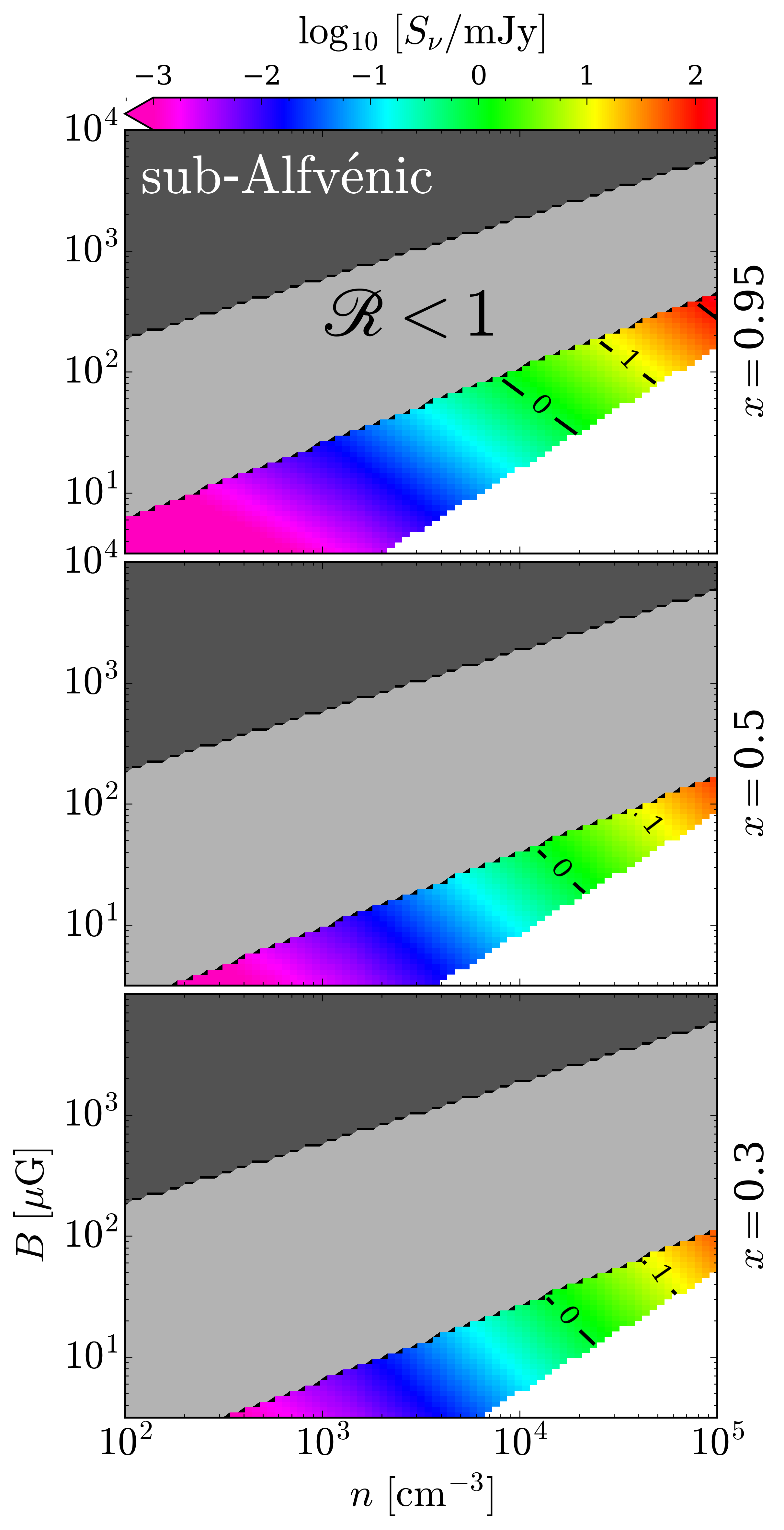
Figure 6: Flux density, $S_{\nu}$, for $T=7500$ K, $U=40$ km s^-1, $L=0.5$ pc, $\nu=300$ MHz, and $\theta_{b}=10\arcsec$ in parameter space $(n,B)$ for three different values of ionisation fraction as labelled on right-hand side of each subplot. Dark and light grey-shaded areas in each subplot show the region of the parameter space where the condition of super-Alfvénic flow and ion-neutral coupling is not satisfied, respectively. Solid black lines in each subplot show the iso-flux density at 1 and 10 mJy in logarithmic scale (from the bottom up).