Diagnosing Cosmic Ray Modified Shocks with H $\alpha$ Polarimetry

Abstract

A novel diagnostic of cosmic-ray modified shocks by polarimetry of H $\alpha$ emissions is suggested. In a cosmic-ray modified shock, the pressure of cosmic rays is sufficiently high compared to the upstream ram pressure to force the background plasma to decelerate (measured in the shock rest frame). Simultaneously, a fraction of the hydrogen atoms co-existing in the upstream plasma collide with the decelerated protons and undergo charge-exchange reactions. As a result, hydrogen atoms with the same bulk velocity of the decelerated protons are generated. We show that when the shock is observed from edge-on, the H $\alpha$ radiated by these upstream hydrogen atoms is linearly polarized with a sizable degree of a few per cent as a result of resonant scattering of Ly $\beta$. The polarization direction depends strongly on the velocity modification; the direction is parallel to the shock surface for the case of no modification, while the direction is parallel to the shock velocity for the case of a modified shock.

1 Introduction

Supernova remnant (SNR) shock waves are believed to be the origin of Galactic cosmic-rays (CRs). If this is the case, they should produce a sufficient amount of CRs to explain the CR energy density measured in the vicinity of the Earth (e.g. $\simeq 1~{}{\rm eV~{}cm^{-3}}$ for CR protons) and should accelerate CR-nuclei up to at least $10^{15.5}~{}{\rm eV}$ (the so-called knee energy). The former can be estimated by measurements of the energy loss rate of shocks due to CR acceleration (e.g. Shimoda et al., 2018a; Hovey et al., 2018, and references therein). The latter is one of the most actively discussed topics using combinations of wide band observations such as $\gamma$-ray, X-ray and radio wave (e.g. Archambault et al., 2017; Laming, 2015, for Tycho’s SNR and references therein). Although such investigations are widely reported on, these two requirements are still open issues.

From a theoretical point view, the acceleration efficiency of CRs and the maximum energy of CRs realized in SNR shocks are related to each other. The most generally accepted mechanism for CR acceleration is diffusive shock acceleration (DSA, e.g. Bell, 1978; Blandford & Ostriker, 1978). In the DSA mechanism, particles bouncing back and forth between the upstream and downstream regions are accelerated. This behaviour is quantified by their spatial diffusion coefficient, which depends on the nature of magnetic disturbances (see, e.g. Blandford & Eichler, 1987, for review). In order to accelerate CR nuclei to the knee energy in SNR shocks, an extremely disturbed magnetic field with a strength of $\sim 100~{}{\rm\mu G}$ is required in the upstream region (e.g. Lagage & Cesarsky, 1983a, b). However, the typical strength of the magnetic field in the local interstellar medium (upstream region) is estimated to be at most $\sim 10~{}{\rm\mu G}$ (e.g. Myers, 1978; Beck, 2001). Motivated by this issue of magnetic field strength, Bell (2004) provided a linear analysis of parallel shocks efficiently accelerating CR protons. He showed that the upstream magnetic field is amplified by the effects of a back reaction from the accelerated protons themselves. This amplification is called the Bell instability whose growth rate is proportional to the square root of the CR energy density. On the other hand, it is also known that the CRs leaking to the upstream region can have a comparable pressure compared to the ram pressure of the upstream background protons. As a result, measured in the rest frame of shock, the background thermal protons are decelerated by the pressure gradient due to CRs before entering the shock front (e.g. Drury & Voelk, 1981; Drury & Falle, 1986). Such a shock is called a CR modified shock. Hence, when the CR acceleration efficiency is sufficiently high, in other words, when the CR pressure or energy density is large enough, the DSA mechanism is regulated by the CRs themselves via the effects of the back reaction on the background plasma (see also Laming et al., 2014, for more detail).

The CR modified shock scenario discussed above is often employed in SNR shocks to explain the spectral energy distribution (SED) of non-thermal emissions (see, e.g. Archambault et al., 2017). However, current SED fitting can not discriminate between the acceleration models. For example, whether TeV band $\gamma$-rays originate from the CR nuclei or CR electrons is representative of the problem. This issue mainly depends on the uncertainties of structure of ambient medium and uncertainties of the details of plasma physics including the back reaction rather than the quality of the observational SED data. Indeed, Inoue et al. (2012) and Inoue (2019) showed that the multiphase structure of the interstellar medium as a consequence of thermal instability results in the same form of $\gamma$-ray spectrum for the cases of CR nuclei and CR electrons. Thus, we need other constraints for further investigations of CR acceleration in SNR shocks.

Observation of the velocity modification of upstream protons, which has unfortunately never been done, would provide us with a novel insight into the CR acceleration process because the degree of modification and the length scale of the modified region would reflect the CR acceleration efficiency and the diffusion length of CRs respectively (see, e.g. Berezhko & Ellison, 1999, for a simplified case). Note that this means that we should know the condition of the background upstream plasma rather than the CRs themselves to reveal the physics of the acceleration. The plasma conditions around the shock can be investigated through observations of the hydrogen Balmer lines, especially H $\alpha$ (e.g. Chevalier et al., 1980; Raymond, 1991; Smith et al., 1994). Indeed, the H $\alpha$ emissions from the upstream region have been observed in actual SNRs (e.g. Lee et al., 2007; Katsuda et al., 2016; Knežević et al., 2017). This upstream H $\alpha$ can originate from the absorption of Ly $\beta$ photons radiated from the downstream region (e.g. Shimoda & Laming, 2019). The absorption of Ly $\beta$ results in an excited hydrogen atom in the 3p state followed by the excited atom emitting H $\alpha$ due to the transition from 3p to 2s with a probability of 0.12 (otherwise it re-emits Ly $\beta$). Note that this is a scattering of an electromagnetic wave and therefore the H $\alpha$ should have a net linear polarization. For the case of a CR modified shock, the decelerated protons can interact with hydrogen atoms and be changed to hydrogen atoms by the charge-exchange reaction, H$+$p$\rightarrow$p$+$H, where H and p denote the hydrogen atom and the proton, respectively (Ohira & Takahara, 2010). Since these newly generated hydrogen atoms have a different mean velocity compared to pre-existing hydrogen atoms, properties of the Ly $\beta$-H $\alpha$ conversion in the upstream region differs from the case of no modification. In this paper, we show that the velocity modification can be measured by polarimetry of H $\alpha$: linear polarization parallel to the shock surface is observed for the case of no CR, while polarization perpendicular to the surface is observed for the case of a modified shock.

This paper is organized as follows: in Section 2, we provide basic concepts for the linear polarization degree and its direction for H $\alpha$ resulting from the Ly $\beta$ scattering. In section 3, we estimate the polarization of H $\alpha$ for the cases of no CR precursor, only an electron heating precursor, and a proton decelerated precursor accompanied by electron heating based on the sophisticated atomic population calculations of Shimoda & Laming (2019). Finally, we summarize our results and discuss future prospects.

2 Basic concepts for Polarization of Scattered Line

Here we consider the polarization of H $\alpha$ resulting from the scattering of Ly $\beta$ following the Rayleigh scattering formulas (e.g. Chandrasekhar, 1960). We treat the radiation transfer problem in a steady state slab geometry. The slab corresponds to the SNR shock front. The shock is plane-parallel to the $x$-$y$ plane and axially symmetric about the $z$-axis. Thus, the specific intensity $I_{\rm\nu,\mu}$ at a position $z$ depends only on the direction of propagation making an angle $\theta$ to the $z$-axis. The label of the direction is $\mu\equiv\cos\theta$ and $\nu$ is the frequency of the photon.

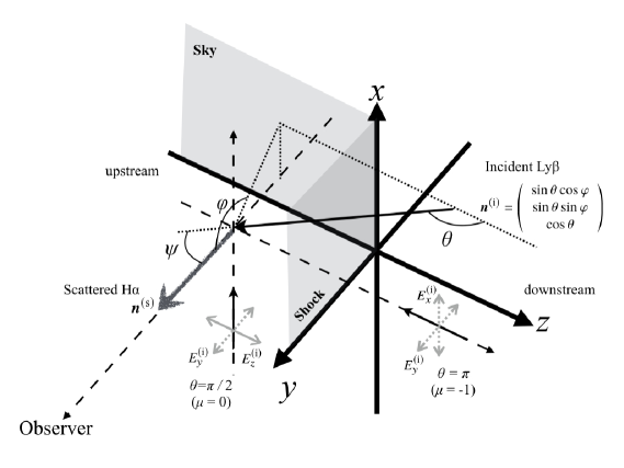
Figure 1: Schematic diagram of an SNR shock. The shock is plane and parallel to the $x$-$y$ plane. We observe the shock from the $y$ direction. The two gray sheets represent the shock surface and the sky. The thick black arrows indicate the incident Ly $\beta$ which propagates in the direction of $\bm{n}^{\rm(i)}=(\sin\theta\cos\varphi,\sin\theta\sin\varphi,\cos\theta)$. The fuzzy arrow indicates the scattered H $\alpha$ in the direction of $\bm{n}^{\rm(s)}=(0,1,0)$. $\bm{n}^{\rm(i)}$ makes an angle $\psi$ with $\bm{n}^{\rm(s)}$. The gray two-way arrows associated with the incident Ly $\beta$ in the direction $\theta=\pi/2$ and $\theta=\pi$ indicate the components of electric field. The dotted two-way arrows indicate the $x$ or $y$ component which may responsible for the excitation of 3p_3/2 state, resulting in the negative polarization (along the $x$-axis). The solid two-way arrow indicates the $z$ component which remains before and after the scattering, giving the positive polarization (along the $z$-axis). The broken and dotted lines are auxiliary lines.

Figure 1 shows a schematic diagram of the shock. Ly $\beta$ is incident from the direction of

$$\bm{n}^{\rm(i)}=\left(\begin{array}[]{c}\sin\theta\cos\varphi\\ \sin\theta\sin\varphi\\ \cos\theta\end{array}\right),$$ (4)

and it is scattered as H $\alpha$ in the direction of

$$\bm{n}^{\rm(s)}=\left(\begin{array}[]{c}0\\ 1\\ 0\end{array}\right).$$ (8)

The scattering angle is defined as

$$\cos\psi=\bm{n}^{\rm(i)}\cdot\bm{n}^{\rm(s)}=\sin\theta\sin\varphi.$$ (9)

In this paper, we fix our line of sight along the $y$-axis so the $z$-$x$ plane corresponds to the sky. Thus, the linear polarization of scattered H $\alpha$ is characterized by its $z$ and $x$ components of electric field, $E_{z}^{\rm(s)}$ and $E_{x}^{\rm(s)}$. In addition, we suppose the optically thin limit for H $\alpha$. This can be valid for an SNR shock propagating into a medium with a number density of $<30~{}{\rm cm^{-3}}$ (Shimoda & Laming, 2019). The polarization is described by the intensity components [erg cm^-2 s^-1 Hz^-1 str^-1]:

$$I_{\nu,z}^{\rm(s)} \equiv a\left<E_{z}^{\rm(s)*}E_{z}^{\rm(s)}\right>,$$ (10)

and,

$$I_{\nu,x}^{\rm(s)} \equiv a\left<E_{x}^{\rm(s)*}E_{x}^{\rm(s)}\right>,$$ (11)

where the asterisk ^∗ indicates the complex conjugate, $\left<...\right>$ means a long time average and the factor $a$ is a dimensional positive constant whose actual value is not important in this paper. Then, the Stokes parameters are defined as

$$I_{\nu}^{\rm(s)} \equiv I_{\nu,z}^{\rm(s)}+I_{\nu,x}^{\rm(s)},$$ (12)

$$Q_{\nu}^{\rm(s)} \equiv I_{\nu,z}^{\rm(s)}-I_{\nu,x}^{\rm(s)}$$ (13)

and,

$$U_{\nu}^{\rm(s)} \equiv a\left<E_{z}^{(s)*}E_{x}^{(s)}\right>-a\left<E_{x}^{(s)*}E_{z}^{(s)}\right>.$$ (14)

Here we omit the label $\mu$ because our line of sight is fixed along the $y$-axis. A positive $Q_{\nu}^{\rm(s)}$ indicates a linear polarization along the $z$-axis (perpendicular to the shock surface), while a negative $Q_{\nu}^{\rm(s)}$ indicates polarization along the $x$-axis (parallel to the shock surface). For the incident Ly $\beta$, we use similar notations. Note that since we consider linear polarization only, the Stokes $V$ is omitted.

In Rayleigh scattering, the polarization of scattered light is given with respect to the scattering plane that is defined by $\bm{n}^{\rm(i)}$ and $\bm{n}^{\rm(s)}$. We denote the component parallel to this plane as $\parallel$ and the component perpendicular to it as $\perp$. Then, we obtain the scattered intensities as (Chandrasekhar, 1960)

$$\left(\begin{array}[]{c}I_{\nu,\parallel}^{\rm(s)}\\ I_{\nu,\perp}^{\rm(s)}\\ \tilde{U}_{\nu}^{\rm(s)}\end{array}\right)=N_{\rm R}\int{\cal R}\left(\begin{array}[]{c}I_{\nu,\mu,\parallel}^{\rm(i)}\\ I_{\nu,\mu,\perp}^{\rm(i)}\\ \tilde{U}_{\nu,\mu}^{\rm(i)}\end{array}\right){\rm d}\Omega^{\rm(i)},$$ (21)

where ${\rm d}\Omega^{\rm(i)}=\sin\theta{\rm d}\theta{\rm d}\varphi$ is the solid angle element for the incident Ly $\beta$. The superscript (i) indicates the incident Ly $\beta$. The Stokes $U$ of the scattered H $\alpha$ (incident Ly $\beta$) are $\tilde{U}_{\nu}^{\rm(s)}$ ($\tilde{U}_{\nu}^{\rm(i)}$) and are defined by the components of electric field $\parallel$ and $\perp$. The normalization factor we discuss later in Section 3 is $N_{\rm R}$. The phase matrix ${\cal R}$ gives the conservation of angular momentum between the photons and bound electron before and after the scattering (i.e. the polarization), which depends on the properties of atomic transitions in general. In our case, the Ly $\beta$-H $\alpha$ conversion, the relevant atomic transitions are from 1s_1/2 to 3p_1/2 and to 3p_3/2 of hydrogen atoms. Note that the subscript $j$ (1/2 and 3/2) denotes the excited bound electron’s angular momentum. According to Hamilton (1947) and Chandrasekhar (1960), the matrices for the cases of 3p_1/2 ($\Delta j=1/2-1/2=0$) and 3p_3/2 ($\Delta j=3/2-1/2=1$) are given by

$${\cal R}=\left(\begin{array}[]{ccc}1&1&0\\ 1&1&0\\ 0&0&0\end{array}\right)$$ (25)

and

$${\cal R}=\frac{3}{4}\left(\begin{array}[]{ccc}\cos^{2}\psi&0&0\\ 0&1&0\\ 0&0&\cos\psi\end{array}\right)+\frac{1}{4}\left(\begin{array}[]{ccc}1&1&0\\ 1&1&0\\ 0&0&0\end{array}\right),$$ (32)

respectively. We have to transform the polarization with respect to the scattering plane given by Eq. (21) to one with respect to the $z$-$x$ plane. Let $\tilde{\theta}$ be an angle between the $z$-axis and the axis along the parallel component of electric field:

$$\tan\tilde{\theta}=\frac{\sin\tilde{\theta}}{\cos\tilde{\theta}}=\frac{\sin\theta\cos\varphi}{\cos\theta}.$$ (33)

Note that since the scattering plane includes $\bm{n}^{\rm(s)}=(0,1,0)$, the parallel and perpendicular axes are always in the $z$-$x$ plane. The parallel component of electric field is written as $\bm{E}_{\parallel}=E_{\parallel}\left(\cos\tilde{\theta},\sin\tilde{\theta}\right)$. Similarly, $\bm{E}_{\perp}=E_{\perp}\left(\sin\tilde{\theta},\cos\tilde{\theta}\right)$. Thus, we obtain the intensities measured along the $z$-axis and $x$-axis, respectively,

$$I_{z}=I_{\parallel}\cos^{2}\tilde{\theta}+I_{\perp}\sin^{2}\tilde{\theta},$$ (34)

$$I_{x}=I_{\parallel}\sin^{2}\tilde{\theta}+I_{\perp}\cos^{2}\tilde{\theta},$$ (35)

and

$$U=\left(I_{\parallel}-I_{\perp}\right)\sin 2\tilde{\theta}+\tilde{U}\cos 2\tilde{\theta},$$ (36)

where we omit the notations $\nu,$ $\mu$, (s) and (i).

Hydrogen atoms in the 3p_1/2 state yield completely unpolarized H $\alpha$: $I_{\nu,z}^{\rm(s)}=I_{\nu,x}^{\rm(s)}$ and $U_{\nu}^{\rm(s)}=0$. Note that the polarization of a photon can be characterized by the specific component of its angular-momentum (i.e. spin) along its direction of travel, and is responsible for the transverse components of the electric fields. For example, we define that a completely left-handed (right-handed) circularly polarized photon propagating along the $z$ axis has a $z-$component of $+1$ ($-1$). In general, the light is partially polarized because not all photons are emitted with the same angular momentum $z$-component. The transitions from 1s_1/2 to 3p_1/2 are induced by the absorption equal numbers of left and right circularly polarized photons with a net component of zero, and the subsequent transitions from 3p_1/2 to 2s_1/2 emit photons with the zero net-component so as to satisfy the conservation of angular momentum. Thus, the scattered H $\alpha$ is completely unpolarized in this case.

In the following, we assume that the incident Ly $\beta$ is always completely unpolarized for simplicity (c.f. Laming, 1990; Shimoda et al., 2018a). Thus,

$$I_{\nu,\mu,\parallel}^{\rm(i)}=I_{\nu,\mu,\perp}^{\rm(i)}=\frac{I_{\nu,\mu}^{\rm(i)}}{2}$$ (37)

and

$$\tilde{U}_{\nu,\mu}^{\rm(i)}=0.$$ (38)

Note that 88 per cent of hydrogen atoms in the 3p state emit Ly $\beta$ again (not H $\alpha$). This re-emitted Ly $\beta$ can be polarized and will be immediately re-absorbed by other hydrogen atoms. After repeating a few times this Ly $\beta$-Ly $\beta$ scattering, the 3p state hydrogen atom emits H $\alpha$ (the Ly $\beta$-H $\alpha$ conversion occurs). During this trapping of Ly $\beta$, the net polarization of Ly $\beta$ may be washed out. Hence, we follow the assumption that all of the incident Ly $\beta$ is completely unpolarized. 

For the case of 3p_3/2 ($\Delta j=1$), the polarization of H $\alpha$ is given by

$$I_{\nu}^{\rm(s)}=N_{\rm R}\int_{-1}^{1}I_{\nu,\mu}^{\rm(i)}\left(\frac{17}{16}-\frac{3}{16}\mu^{2}\right){\rm d}\mu,$$ (39)

$$Q_{\nu}^{\rm(s)}=N_{\rm R}\int_{-1}^{1}I_{\nu,\mu}^{\rm(i)}\left(\frac{3}{16}-\frac{9}{16}\mu^{2}\right){\rm d}\mu,$$ (40)

and $U_{\nu}^{\rm(s)}=0$, where we use the notation $\mu=\cos\theta$ and include the numerical factor coming from the integration by $\varphi$ in $N_{\rm R}$. Since the specific component of angular momentum varies, the scattered H $\alpha$ can be polarized, unlike the case of 3p_1/2. The sign of $Q_{\nu}^{\rm(s)}$ refers whether the polarization is along the $z$-axis (positive) or the $x$-axis (negative).

We discuss the polarization properties of scattered H $\alpha$ for the transition from 1s_1/2 to 3p_3/2. First, when all of the photons are incident from the direction $|\mu|=1$ (Figure 1 shows the case of $\mu=-1$), the Stokes $Q_{\nu}^{\rm(s)}$ becomes negative (polarized along the $x$-axis). This is the usual polarization property for the scattering of electromagnetic (transverse) waves. Note that this situation gives a maximum degree of polarization $\simeq-0.43$. On the other hand, for the case of $\mu=0$ (Figure 1 shows the case of incident along the $x$-axis), we observe a positive polarization with $\simeq 0.18$ degree. This is also the usual property of electromagnetic wave scattering. The polarization degree reflects the nature of angular momentum in the atomic transition  (the laws of conservation, commutation and synthesis, see e.g. Hamilton, 1947, for details). 

Inside a uniform, isotropically emitting medium the incident intensity is,

$$I_{\nu,\mu}^{\rm(i)}=S_{\nu}(1-{\rm e}^{-\frac{\tau_{\nu}}{|\mu|}}),$$ (41)

where $S_{\nu}$ and $\tau_{\nu}$ are $\mu$–independent source function and optical depth respectively. The Stokes parameters are

$$I_{\nu}^{\rm(s)} = N_{\rm R}\int_{-1}^{1}S_{\nu}(1-{\rm e}^{-\frac{\tau_{\nu}}{|\mu|}})\left(\frac{17}{16}-\frac{3}{16}\mu^{2}\right){\rm d}\mu,$$ (42)

$$= N_{\rm R}S_{\nu}\left[2-\int_{-1}^{1}{\rm e}^{-\frac{\tau_{\nu}}{|\mu|}}\left(\frac{17}{16}-\frac{3}{16}\mu^{2}\right){\rm d}\mu\right],$$

and

$$Q_{\nu}^{\rm(s)} = N_{\rm R}\int_{-1}^{1}S_{\nu}(1-{\rm e}^{-\frac{\tau_{\nu}}{|\mu|}})\left(\frac{3}{16}-\frac{9}{16}\mu^{2}\right){\rm d}\mu,$$ (43)

$$= -N_{\rm R}S_{\nu}\int_{-1}^{1}{\rm e}^{-\frac{\tau_{\nu}}{|\mu|}}\left(\frac{3}{16}-\frac{9}{16}\mu^{2}\right){\rm d}\mu.$$

Thus, the polarization degree is

$$\frac{Q_{\nu}^{\rm(s)}}{I_{\nu}^{\rm(s)}}=\frac{-\int_{-1}^{1}{\rm e}^{-\frac{\tau_{\nu}}{|\mu|}}\left(\frac{3}{16}-\frac{9}{16}\mu^{2}\right){\rm d}\mu}{2-\int_{-1}^{1}{\rm e}^{-\frac{\tau_{\nu}}{|\mu|}}\left(\frac{17}{16}-\frac{3}{16}\mu^{2}\right){\rm d}\mu}.$$ (44)

It can be expressed as

$$\frac{Q_{\nu}^{\rm(s)}}{I_{\nu}^{\rm(s)}} = \frac{-3A(\tau_{\nu})+9B(\tau_{\nu})}{16-17A(\tau_{\nu})+3B(\tau_{\nu})},$$ (45)

$$A(\tau_{\nu}) = {\rm e}^{-\tau_{\nu}}-\tau_{\nu}E_{1}(\tau_{\nu}),$$ (46)

$$B(\tau_{\nu}) = \frac{{\rm e}^{-\tau_{\nu}}}{6}\left(\tau_{\nu}{}^{2}-\tau_{\nu}+2\right)-\frac{\tau_{\nu}{}^{3}E_{1}(\tau_{\nu})}{6},$$ (47)

where

$$E_{1}(\tau_{\nu})=\int_{\tau_{\nu}}^{\infty}\frac{{\rm e}^{-\alpha}}{\alpha}{\rm d}\alpha,$$ (48)

is the exponential integral.

Figure 2: The polarization degree of scattered H $\alpha$ at the line centre. Note that we consider only the transition from 3p_3/2 to 2s_1/2 here. The solid line is the case of a uniform, isotropically emitting medium in which the intensity of Ly $\beta$ is given by Eq. (41). The dots represent the case of an anisotropic radiation field modeling the SNR shock. Here we set $I_{\nu,{\rm B}}=10S_{\nu}$ in Eq. (50).

Figure 2 shows the polarization degree at the line centre (see solid line). Since the intensity of Ly $\beta$ incident from $\mu\approx 0$ is stronger than from $\mu\approx 1$ at small $\tau_{\nu}$, in other words, since the incident ‘photon beam’ is elongated along the $x$-axis, the polarization degree is positive. For $\tau_{\nu}\gg 1$, the radiation field becomes isotropic (i.e. $I_{\nu,\mu}^{\rm(i)}\approx S_{\nu}$) and thus the polarization is zero.

As discussed above, the polarization of the scattered line depends on the anisotropy of the radiation field. Even if we consider a uniform, isotropically emitting medium, the anisotropy arises from the effects of attenuation and the scattered line has net polarization. For SNR shocks, hydrogen atoms in the upstream region are illuminated by Ly $\beta$ radiated from the downstream region. Thus, the radiation field is quite anisotropic at the shock (e.g. Figure 7 of Shimoda & Laming, 2019). This situation may be modeled by

$$I_{\nu,\mu}^{\rm(i)}=I_{\nu,{\rm B}}{\rm e}^{-\frac{\tau_{\nu}}{|\mu|}}+S_{\nu}(1-{\rm e}^{-\frac{\tau_{\nu}}{|\mu|}}),$$ (49)

where $I_{\nu,{\rm B}}$ is the $\mu$-independent intensity of Ly $\beta$ from the downstream region, and $\tau_{\nu}$ is now the optical depth outside the shock. Then, the polarization degree becomes

$$\frac{Q_{\nu}^{\rm(s)}}{I_{\nu}^{\rm(s)}} = \frac{\left(I_{\nu,{\rm B}}-S_{\nu}\right)\left(3A(\tau_{\nu})-9B(\tau_{\nu})\right)}{16S_{\nu}+\left(I_{\nu,{\rm B}}-S_{\nu}\right)\left(17A(\tau_{\nu})-3B(\tau_{\nu})\right)}.$$ (50)

Figure 2 shows the case of $I_{\nu,{\rm B}}=10S_{\nu}$ (see dots), giving ‘negative’ polarization. Note that if the value of $S_{\nu}$ is absolutely equal to zero, the polarization degree becomes $-0.43$ at $\tau_{\nu}\rightarrow\infty$. In other words, if $S_{\nu}$ has a very small but finite value, the degree becomes zero at which $I_{\nu,{\rm B}}{\rm e}^{-\frac{\tau_{\nu}}{\mu}}\ll S_{\nu}$. Hence, in actual SNR shocks, H $\alpha$ can have a sizable, ‘negative’ polarization degree in the upstream region.

For the CR modified shock, the upstream hydrogen atoms can be decelerated before entering the shock front as a consequence of charge-exchange reactions with decelerated protons. This ‘deceleration’ is measured in the shock rest frame. In the observer rest frame (far upstream rest frame), the particles are accelerated towards the far upstream region where the CR back reactions cease. Thus, the atoms in the far upstream region ‘see’ blue-shifted Ly $\beta$ radiated by the decelerated atoms. As a result, the optical depth depends strongly on the direction cosine $\mu$. Because the Ly $\beta$ incident from $\mu\approx 0$ are seen as not shifted, the scattering of the $\mu\approx 0$ photons becomes dominant, giving a ‘positive’ polarization.

In actual SNR shocks, unfortunately, the radiation line transfer problem including the polarization is quite complex even if there is no shock modification. Hence, using the latest radiative line transfer model of SNR shocks constructed by Shimoda & Laming (2019) and making several simplifications, we estimate the polarization of H $\alpha$ for both cases of modified/unmodified shock in this paper.

3 Model

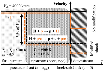
Figure 3: Schematic illustration of the shock models considered in this paper. The vertical axis shows the velocities of hydrogen atoms and protons measured in the shock rest frame. The horizontal axis is the $z$ axis. The shock (or sub-shock for the modified shock case) is located at $z=0$. The solid lines indicate the cases of no velocity modification, while the broken lines indicate the case of the modified shocks. The orange lines are the mean velocity of protons and the black lines are the mean velocity of hydrogen atoms, respectively. The precursor front is located at $z=z_{\rm pre}$ at which the electrons are heated up to $10^{6}$ K and the protons are being decelerated to have a mean velocity of $0.95V_{\rm sh}$. Some of hydrogen atoms having the same bulk velocity as the protons emerge from charge-exchange reactions.

We estimate the polarization of H $\alpha$ from the upstream region of SNR shocks with fixed shock velocity, $V_{\rm sh}=4000~{}{\rm km~{}s^{-1}}$, far upstream temperature, $T_{0}=6000$ K, and preshock ionization degree, $\chi_{0}=0.5$, for the following three cases: (i) no particles leaking to the upstream region which is the same situation as in Shimoda & Laming (2019), (ii) an electron heating precursor with temperature of $10^{6}$ K due to CRs but no velocity modifications following Laming et al. (2014), (iii) in addition to the electron heating precursor, there are decelerated protons, but with no proton heating. Figure 3 summarises these three cases. We assume that the velocity modification is $5$ per cent of $V_{\rm sh}$ (i.e. $200~{}{\rm km~{}s^{-1}}$) and that the downstream values are given by usual the Rankine-Hugoniot relations for simplicity. Note that the downstream electron temperature is fixed at 10 per cent of proton temperature ($T_{\rm e}\simeq 3~{}{\rm keV}$).

In the radiation line transfer model of Shimoda & Laming (2019), the shock geometry is the same as in Figure 1. For the radiation transfer problem, they set the two free escape boundaries for photons upstream and downstream of the shock. The plasma they consider consists of protons, electrons and hydrogen atoms. Note that bremsstrahlung radiation, emission from the SNR ejecta and any other external radiation sources are neglected. The excitation levels of hydrogen atom are considered up to 4f. Their model did not consider the existence of a precursor. Therefore, we additionally solve the ionization structure of hydrogen for the precursor cases.

For case (ii), with only an electron heating precursor, we solve the ionization structure of the upstream hydrogen in the shock rest frame with the following equations

$$\frac{\partial n_{\rm H}^{0}}{\partial z}=-n_{\rm H}^{0}\frac{C_{\rm I}}{V_{\rm sh}},$$ (51)

and

$$\frac{\partial n_{\rm p}}{\partial z}=n_{\rm H}^{0}\frac{C_{\rm I}}{V_{\rm sh}},$$ (52)

where $n_{\rm H}^{0}$ is the number density of hydrogen atoms that have not experienced the charge-exchange reactions. The number density of protons is $n_{\rm p}$ and $C_{\rm I}$ is the ionization rate. For the modified shock case (iii), the ionization structure in the precursor region is given by

$$\frac{\partial n_{\rm H}^{0}}{\partial z}=-n_{\rm H}^{0}\frac{C_{\rm I}+C_{\rm CX}}{V_{\rm sh}},$$ (53)

$$\frac{\partial n_{\rm H}^{1}}{\partial z}=\frac{n_{\rm H}^{0}C_{\rm CX}-n_{\rm H}^{1}C_{\rm I}}{u_{1}},$$ (54)

and

$$\frac{\partial n_{\rm p}}{\partial z}=\left(n_{\rm H}^{0}+n_{\rm H}^{1}\right)\frac{C_{\rm I}}{u_{1}}.$$ (55)

where $n_{\rm H}^{1}$ is the number density of hydrogen atoms that have experienced charge-exchange reactions with the decelerated protons. The bulk velocity of the decelerated protons and that of the hydrogen atoms having undergone charge-exchange reactions is $u_{1}$. The rate of charge-exchange reactions for the relative velocity of $200~{}{\rm km~{}s^{-1}}$ is $C_{\rm CX}\simeq 4.59\times 10^{-8}(n_{\rm p}/{\rm 1~{}cm^{-3}})~{}{\rm s^{-1}}$ (Janev & Smith, 1993; Janev et al., 2003). In the following, the total number density of hydrogen atoms is denoted as $n_{\rm H}=n_{\rm H}^{0}+n_{\rm H}^{1}$. Note that $n_{\rm H}^{1}=0$ for the cases (i) and (ii) because there are no decelerated protons. The ionization structure of the downstream region is given by the same formulations as in Shimoda & Laming (2019). Note that the velocity distribution function of all particles are shifted Maxwellians.

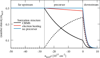
Figure 4: The ionization structure of the hydrogen atoms. The blue, red and black lines indicate the cases of no precursor (i), only the electron heating precursor (ii), and the electron heating precursor with decelerated protons (iii), respectively. The solid lines are the number density of hydrogen atoms that have not experienced a charge-exchange reaction in the precursor region, $n_{\rm H}^{\rm 0}$. The broken line is the number density of hydrogen atoms that have experienced a charge-exchange reaction with the decelerated protons in the precursor region, $n_{\rm H}^{\rm 1}$. The vertical thin lines at $n_{\rm tot,0}z\simeq-27\times 10^{15}~{}{\rm cm^{-2}}$ and $n_{\rm tot,0}z\simeq 0~{}{\rm cm^{-2}}$ indicate the locations of the precursor front and the shock front, respectively.

Figure 4 shows the ionization structure of hydrogen. The results are normalized by the total number density $n_{\rm tot,0}=n_{\rm p}+n_{\rm H}$. Here we set the precursor front at $n_{\rm tot,0}z_{\rm pre}=0.14V_{\rm sh}/\tilde{C}_{\rm I}$, where $\tilde{C}_{\rm I}=C_{\rm I}/n_{\rm p}\simeq 2.15\times 10^{-9}~{}{\rm cm^{3}~{}s^{-1}}$ is estimated for $T_{\rm e}=10^{6}$ K. The hydrogen atoms in the precursor region are modestly ionized by the heated electrons but most of them experience charge-exchange reactions with the decelerated protons ($n_{\rm tot,0}z_{\rm pre}\simeq 3n_{\rm p}V_{\rm sh}/C_{\rm CX}$).

In order to constrain the velocity modification of shock via the H $\alpha$ emission, the length scale of modification $z_{\rm pre}$ has to be sufficiently larger than the characteristic length of the spatial distribution of the decelerated hydrogen atoms emerging from the charge-exchange reaction with the decelerated protons, $V_{\rm sh}/C_{\rm CX}(\Delta V_{\rm sh})$, where $\Delta V_{\rm sh}\simeq 200~{}{\rm km~{}s^{-1}}$ is the relative velocity of collision particles. In this paper, we show the case of $z_{\rm pre}\simeq 3(n_{\rm p}/n_{\rm tot,0})V_{\rm sh}/C_{\rm CX}$. If the modification comes from CRs accelerated at the shock, the length scale of modification can be given by their diffusion length $l_{\rm diff}\sim D(E)/V_{\rm sh}$, where $D$ and $E$ are the CR diffusion coefficient and energy, respectively. Thus, from the observational condition $l_{\rm diff}\ga 3(n_{\rm p}/n_{\rm tot,0})V_{\rm sh}/C_{\rm CX}$, we obtain

$$D(E) \ga 1.05\times 10^{25}~{}{\rm cm^{-2}~{}s^{-1}}$$

$$\times \left(\frac{V_{\rm sh}}{4000~{}{\rm km~{}s^{-1}}}\right)^{2}\left(\frac{n_{\rm tot,0}}{1~{}{\rm cm^{-3}}}\right)^{-1}\left(\frac{\Delta V_{\rm sh}}{200~{}{\rm km~{}s^{-1}}}\right)^{-1},$$

where we approximate

$$\frac{C_{\rm CX}}{n_{\rm p}}\approx 4.59\times 10^{-8}~{}{\rm cm^{3}~{}s^{-1}}\left(\frac{\Delta V_{\rm sh}}{200~{}{\rm km~{}s^{-1}}}\right).$$

The diffusion coefficient for the interstellar medium, $D_{\rm ISM}(1~{}{\rm GeV})\sim 10^{28}~{}{\rm cm^{2}~{}s^{-1}}$, satisfies this condition. When magnetic disturbances are excited around an SNR shock, we can not currently derive the relevant diffusion coefficient. If we suppose the simplest case, $D(E)\simeq\xi_{\rm B}r_{g}(E)c/3$, where $r_{g}$ is the gyro radius of CR and $\xi_{\rm B}>1$ is the gyro factor characterized by the energy spectrum of magnetic disturbances, we obtain a lower bound for the CR energy $E$ responsible for the velocity modification of

$$E \ga 33~{}{\rm TeV}\frac{1}{\xi_{\rm B}}\times\left(\frac{B}{100~{}{\rm\mu G}}\right)\left(\frac{V_{\rm sh}}{4000~{}{\rm km~{}s^{-1}}}\right)^{2}$$ (57)

$$\times \left(\frac{n_{\rm tot,0}}{1~{}{\rm cm^{-3}}}\right)^{-1}\left(\frac{\Delta V_{\rm sh}}{200~{}{\rm km~{}s^{-1}}}\right)^{-1}.$$

Note that this estimate of $E$ is based on the coefficient at the Bohm limit, $D(E)\simeq r_{g}(E)c/3$, that gives the shortest diffusion length for a given $E$. For Tycho’s SNR, it is implied by the two-point correlation analysis of synchrotron intensity that the energy spectrum of downstream magnetic disturbances has a Kolmogorov-like scaling (Shimoda et al., 2018b).  If this is also true for the upstream disturbances, the gyro factor $\xi_{\rm B}$ may be greater than unity and the lower bound of $E$ may be smaller than $33$ TeV. Note that the acceleration efficiency of CRs can be measured simultaneously by polarimetry of the downstream H $\alpha$ emission (Shimoda et al., 2018a).

We calculate the atomic populations in the same manner as Shimoda & Laming (2019). Then, we obtain the emissivity of H $\alpha$ as

$$j_{\nu,\mu}=\frac{h\nu}{4\pi}\left(n_{\rm H,3s}A_{\rm 3s,2p}\phi_{\nu,\mu}^{\rm 3s,2p}+n_{\rm H,3p}A_{\rm 3p,2s}\phi_{\nu,\mu}^{\rm 3p,2s}\right.$$

$$\left.+n_{\rm H,3d}A_{\rm 3d,2p}\phi_{\nu,\mu}^{\rm 3d,2p}\right),$$ (58)

where $n_{{\rm H},k}$ denotes the number density of hydrogen atoms in the excited state $k$. The spontaneous transition rate and line profile function for the transition from $k$ to $j$ are given by $A_{k,j}$ and $\phi_{\nu,\mu}^{k,j}$, respectively (see Shimoda & Laming, 2019, for details). Here we omit the term for the two-photon decay. This emissivity gives the total intensity of H $\alpha$ including all contributions such as collisional excitation, radiative excitation and cascades from higher levels (up to 4f in our model). Almost all radiative excitation comes from the absorption of Ly $\beta$, which populates $n_{\rm H,3p}$.

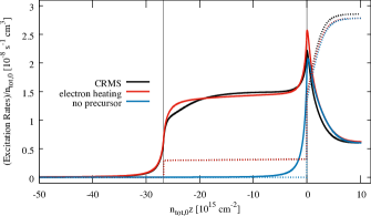
Figure 5: Radiative excitation rate for the transition from 1s to 3p (solid lines) and total collisional excitation rate for the transitions from 1s to 3s, 3p and 3d (dots). The blue, red and black lines indicate the cases of no precursor (i), only an electron heating precursor (ii), and the electron heating precursor with decelerated protons (iii), respectively. The vertical thin lines at $n_{\rm tot,0}z\simeq-27\times 10^{15}~{}{\rm cm^{-2}}$ and $n_{\rm tot,0}z\simeq 0~{}{\rm cm^{-2}}$ indicate the locations of the precursor front and the shock front, respectively.

Figure 5 shows the radiative rate for the transition from 1s to 3p and the total collisional rate of the transitions from 1s to 3s, 3p and 3d. The radiative excitation dominates over the collisional excitation in the upstream region because the Lyman lines are trapped. Thus, in the upstream region, most of H $\alpha$ photons arise from the Ly $\beta$-H $\alpha$ conversion. In this paper, for calculating the Stokes $Q$ of H $\alpha$, we approximate that all of the 3p-state hydrogen atoms arise from Ly $\beta$ absorption. Hence, we obtain

$$n_{\rm H,3p}=n_{\rm H,3p_{3/2}}+n_{\rm H,3p_{1/2}}\approx\left(1+\frac{f_{\rm 1s,3p_{1/2}}}{f_{\rm 1s,3p_{3/2}}}\right)n_{\rm H,3p_{3/2}},$$ (59)

where $f_{\rm 1s,3p_{1/2}}=0.026381$ and $f_{\rm 1s,3p_{3/2}}=0.052761$ are the oscillator strengths for the transitions from 1s to 3p_1/2 and to 3p_3/2, respectively (Wiese & Fuhr, 2009). Since we suppose the optically thin limit for H $\alpha$, the Stokes $I$ of the scattered H $\alpha$ is given by $I_{\nu}^{\rm(s)}=j_{\nu,0}^{\rm 3p_{3/2},2s}L$, where $L$ is a path length along the line of sight and $j_{\nu,\mu}^{k,j}$ is the emissivity for the transition from $k$ to $j$. Note that our line of sight is fixed along the $y$-axis ($\mu=0$). Thus, we obtain the normalization factor of the Rayleigh scattering as

$$N_{\rm R}=\frac{\frac{h\nu}{4\pi}n_{\rm H,3p_{3/2}}A_{\rm 3p,2s}\phi_{\nu,\mu}^{\rm 3p,2s}L}{\int_{-1}^{1}I_{\nu,\mu}^{\rm(i)}\left(\frac{17}{16}-\frac{3}{16}\mu^{2}\right){\rm d}\mu}.$$ (60)

Here we estimate the intensity of Ly $\beta$ in the scattering as

$$I_{\nu,\mu}^{\rm(i)}(z)=I_{\nu,\mu}^{\rm Ly\beta}(z){\rm exp}\left[{-\frac{k_{\nu,\mu}(z)\Delta z}{|\mu|}}\right],$$ (61)

where $k_{\nu,\mu}$ is the absorption coefficient and $I_{\nu,\mu}^{\rm Ly\beta}$ is the specific intensity of Ly $\beta$. They are the outcome of the atomic population calculations. The spatial resolution of our numerical calculation is $\Delta z$: $k_{\nu,\mu}\Delta z\simeq 0.08$ at the far upstream region. The polarization degree of H $\alpha$, finally, is written as

$$\frac{Q_{\nu}^{\rm(s)}}{I_{\nu,0}} = \frac{N_{\rm R}\int_{-1}^{1}I_{\nu,\mu}^{\rm(i)}\left(\frac{3}{16}-\frac{9}{16}\mu^{2}\right){\rm d}\mu}{j_{\nu,0}L}$$ (62)

$$= \frac{n_{\rm H,3p}A_{\rm 3p,2s}\left(1+\frac{f_{\rm 1s,3p_{1/2}}}{f_{\rm 1s,3p_{3/2}}}\right)^{-1}}{n_{\rm H,3s}A_{\rm 3s,2p}+n_{\rm H,3p}A_{\rm 3p,2s}+n_{\rm H,3d}A_{\rm 3d,2p}}$$

$$\times \frac{\int_{-1}^{1}I_{\nu,\mu}^{\rm Ly\beta}{\rm e}^{-\frac{k_{\nu,\mu}}{|\mu|}\Delta z}\left(\frac{3}{16}-\frac{9}{16}\mu^{2}\right){\rm d}\mu}{\int_{-1}^{1}I_{\nu,\mu}^{\rm Ly\beta}{\rm e}^{-\frac{k_{\nu,\mu}}{|\mu|}\Delta z}\left(\frac{17}{16}-\frac{3}{16}\mu^{2}\right){\rm d}\mu}.$$

Note that this polarization degree includes the effects of collisional excitation, cascades from higher levels and scattering in the case of $\Delta j=0$ (transitions from 1s_1/2 to 3p_1/2 and subsequently to 2s_1/2). In particular, we assume that the precursor collisional excitation and cascades yield completely unpolarized H $\alpha$.

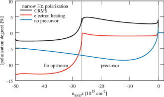
Figure 6: The polarization degree of H $\alpha$. The blue, red and black lines indicate the cases of no precursor (i), only an electron heating precursor (ii), and the electron heating precursor with decelerated protons (iii), respectively. The vertical thin lines at $n_{\rm tot,0}z\simeq-27\times 10^{15}~{}{\rm cm^{-2}}$ and $n_{\rm tot,0}z\simeq 0~{}{\rm cm^{-2}}$ indicate the locations of the precursor front and the shock front, respectively. Positive values correspond to polarization along the $z$-axis, while negative values correspond to polarization along the $x$-axis. Note that these results includes all of atomic levels and processes unlike the result shown in Figure 2.

Figure 6 shows the estimated polarization degree of H $\alpha$ in the upstream region. Here the Stokes parameters are integrated over an interval of frequency corresponding to the Doppler velocity range $-25$ to $25~{}{\rm km~{}s^{-1}}$. As discussed in Section 2, the sign of Stokes $Q$ depends on the velocity modification. In the no precursor case (i), the polarization degree is positive ($\simeq 2$ per cent) in the region close to the shock front where the optical depth of Ly $\beta$ is small. Then, the polarization becomes negative at optical depth $\sim 1$. Since the Ly $\beta$ radiated from the downstream region in the direction of $\mu\approx-1$ (along the $z$-axis) is not so attenuated compared to that radiated along $\mu\approx 0$, the ‘photon beam’ is elongated along the $z$-axis, giving a negative polarization in the region distant from the shock. Note that the polarization at $z\simeq-5\times 10^{16}$ cm is affected by the photon free escape boundary. On the other hand, in the simple electron heating precursor case (ii), the polarization degree is modest ($\simeq-1$ per cent) in the precursor region. This is because the electron heating precursor with no velocity modification yields a uniform, isotropically emitting medium whose polarization property is shown in Figure 2. Note that the polarization degree in front of the shock is $\simeq 1$ per cent in this case (the plots in Figure 6 overlap). In the modified shock case (iii), the polarization is positive with a degree of $\simeq 5$ per cent. The degree of attenuation of Ly $\beta$ photons radiated in the direction $\mu\approx 1$ depends on whether the decelerated/non-decelerated atoms emit/absorb them, while the photons radiated in the direction $\mu\approx 0$ are attenuated by the both populations of atoms. Thus, the photons with $\mu\approx 0$ are efficiently attenuated resulting in positive polarization.

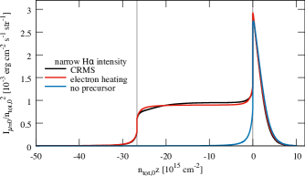
Figure 7: The surface brightness profile of H $\alpha$. The blue, red and black lines indicate the cases of no precursor (i), only the electron heating precursor (ii), and the electron heating precursor with decelerated protons (iii), respectively. The vertical thin lines at $n_{\rm tot,0}z\simeq-27\times 10^{15}~{}{\rm cm^{-2}}$ and $n_{\rm tot,0}z\simeq 0~{}{\rm cm^{-2}}$ indicate the locations of the precursor front and the shock front, respectively.

Figure 7 shows the surface brightness profiles of the frequency-integrated Stokes $I$ for the three cases. In the existence of a precursor, cases (ii) and (iii), the emission from the upstream region is bright and comparable to that from the downstream region. Thus, in an actual observation, the polarization of such precursor emission is detectable. Indeed, Sparks et al. (2015) discovered the polarized H $\alpha$ with a polarization degree of $2.0\pm 0.4$ per cent at SNR SN 1006. Note that the precursor emissions were reported in several cases in the literature (e.g. Lee et al., 2007; Katsuda et al., 2016; Knežević et al., 2017) although their origin is still a matter of debate. Candidates for the origin of these precursor emissions often discussed are the CR precursor, a photoionization precursor and a fast neutral precursor as the result of charge exchange reactions (e.g. Morlino et al., 2012). In particular, by constructing an H $\alpha$ emission model with a fast neutral precursor, Morlino et al. (2012) showed that the fast neutral precursor can contribute up to $\sim 40$ per cent of the total H $\alpha$ emission in the case of complete proton-electron temperature equilibration and $V_{\rm sh}\approx 2500~{}{\rm km~{}s^{-1}}$. Note that the fast neutral precursor also leads to an upstream velocity modification of $\sim 10$ per cent of $V_{\rm sh}$ (Blasi et al., 2012; Ohira, 2012) for $V_{\rm sh}\la 2000~{}{\rm km~{}s^{-1}}$. For $V_{\rm sh}\ga 2000~{}{\rm km~{}s^{-1}}$, the modification hardly occurs because of the rapid decrease of the charge-exchange cross-section at relative velocities $\ga 2000~{}{\rm km~{}~{}s^{-1}}$.

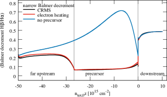
Figure 8: The Balmer decrement (total intensity ratio of H $\beta$ to H $\alpha$). The blue, red and black lines indicate the cases of no precursor (i), only the electron heating precursor (ii), and the electron heating precursor with decelerated protons (iii), respectively. The vertical thin lines at $n_{\rm tot,0}z\simeq-27\times 10^{15}~{}{\rm cm^{-2}}$ and $n_{\rm tot,0}z\simeq 0~{}{\rm cm^{-2}}$ indicate the locations of the precursor front and the shock front, respectively.

Figure 8 is the ratio of the frequency-integrated Stokes $I$ of H $\beta$ to that of H $\alpha$. The ratio does not depend on the existence of a velocity modification, in other words, the net optical depth of the Lyman lines does not depend on the modification. This is also indicated by Figure 5. The reason is that both decelerated and non-decelerated hydrogen atoms survive sufficiently in the precursor region for the absorption of Lyman lines. Thus, the polarimetry of H $\alpha$ is a unique diagnostic for the velocity modification of a shock that is one of the essential predictions for collisionless shocks efficiently accelerating non-thermal particles.

The intensity ratio of H $\beta$ to H $\alpha$ (the so-called Balmer decrement) is often discussed as a ratio in photon counts, which is obtained by multiplying the intensity ratio by a factor of 0.74 (see Shimoda & Laming, 2019). Tseliakhovich et al. (2012) evaluated the ratio in photon counts as $\simeq 0.3$ for the case of only proton direct collisional excitation by assuming Delta-function distributions for protons and hydrogen atoms. Note that this estimate does not include the Lyman-Balmer conversions and cascades from higher levels. Following Tseliakhovich et al. (2012), if we evaluate the downstream ratio in photon counts including the electron direct collisional excitation for a typical relative collision velocity of $\simeq 3/4V_{\rm sh}=3000~{}{\rm km~{}s^{-1}}$, we obtain $\simeq 0.38$. Thus, the ratio at the edge of downstream, $\simeq 0.5\times 0.74\simeq 0.37$, may be almost determined by the collisional excitation for typical relative velocities. Toward the shock front, the ratio becomes smaller due to the Lyman-Balmer conversions. Note that because the oscillator strength of the transition from 1s to 3p is stronger than that to 4p, the Ly $\beta$-H $\alpha$ conversion is more efficient than the Ly $\gamma$-H $\beta$ conversion.

4 Summary and Discussion

We have shown that the polarimetry of H $\alpha$ can be a useful and unique diagnostic of a CR modified shock. The H $\alpha$ emission from the upstream region mainly originates from the Ly $\beta$-H $\alpha$ conversion as a consequence of photon-scattering, even if there is an electron heating precursor yielding collisional excitation. Therefore, the upstream H $\alpha$ is linearly polarized with a polarization degree of $\sim$ a few per cent. The polarization direction (angle) depends strongly on whether there is a velocity modification. For the case of no velocity modification, the polarization direction is parallel to the shock surface. On the other hand, if there are velocity modified hydrogen atoms generated by charge-exchange reactions with the decelerated upstream protons, the direction is perpendicular to the shock surface. Moreover, the upstream surface brightness of H $\alpha$ is comparable to the downstream brightness. Furthermore, we have shown that even if the velocity modification is just 5 per cent of $V_{\rm sh}$, the polarization of H $\alpha$ responds to the modification sensitively. Hence, polarimetry of upstream H $\alpha$ may be realised that will constrain the modification of the shock due to the CR back reactions and bring new insights to particle acceleration in collisionless shocks.

There is another diagnostic for the CR acceleration rate that is often discussed. H $\alpha$ emission with full width at half maximum (FWHM) of $30\mathchar 45\relax 50~{}{\rm km~{}s^{-1}}$ is often observed in SNRs (e.g. Sollerman et al., 2003) and it indicates too high a temperature of $2.5\mathchar 45\relax 5.6~{}{\rm eV}$ for hydrogen atoms to exist if the case of thermal equilibrium holds in the preshock medium. Thus, this anomalous width implies that there is non-thermal pre-heating before shock passage. If the CR acceleration efficiency is really high, such non-thermal heating can occur, for example, via generation and damping of Alfvènic turbulence in the upstream region. Note that the CR back reaction mainly affects charged particles in the plasma but the neutral atoms can be coupled with the affected ions by charge-exchange reactions. Morlino et al. (2013) demonstrated this by a semi-analytical model and showed that the width depends on the maximum energy of the accelerated CRs. On the other hand, Ohira (2016) reported no pre-heating in his hybrid simulation, although his hybrid simulation was generally limited to too short a time scale compared to an actual SNR. Note that his simulation showed the velocity modification with $\sim 10$ per cent of $V_{\rm sh}$. Moreover, for the Cygnus Loop SNR, Medina et al. (2014) pointed out that the FWHM of $\simeq 30~{}{\rm km~{}s^{-1}}$ can be realized in the upstream region by the photo-ionization heating due to radiation from the post-shock or SNR ejecta. This would be accentuated by the photoionization of H₂ molecules, followed by dissociative recombination, whereby the neutral atoms fly apart with the correct energy to produce the observed line width. H₂ emission is observed in the northeast part of Cygnus Loop though it can be from a radiative shock (Graham et al., 1991a; Graham et al., 1991b). Furthermore, Shimoda & Laming (2019) showed that the interaction between the SNR shocks and a dense upstream medium $\ga 30~{}{\rm cm^{-3}}$ can also result in a $30\mathchar 45\relax 50~{}{\rm km~{}^{-1}}$ FWHM due to the scattering of H $\alpha$. Thus, we should still consider carefully whether the width of H $\alpha$ is really firm evidence of efficient CR acceleration.

References

- Archambault et al. (2017) Archambault S., et al., 2017, ApJ, 836, 23
- Beck (2001) Beck R., 2001, Space Sci. Rev., 99, 243
- Bell (1978) Bell A. R., 1978, MNRAS, 182, 147
- Bell (2004) Bell A. R., 2004, MNRAS, 353, 550
- Berezhko & Ellison (1999) Berezhko E. G., Ellison D. C., 1999, ApJ, 526, 385
- Blandford & Eichler (1987) Blandford R., Eichler D., 1987, Phys. Rep., 154, 1
- Blandford & Ostriker (1978) Blandford R. D., Ostriker J. P., 1978, ApJ, 221, L29
- Blasi et al. (2012) Blasi P., Morlino G., Bandiera R., Amato E., Caprioli D., 2012, ApJ, 755, 121
- Chandrasekhar (1960) Chandrasekhar S., 1960, Radiative transfer
- Chevalier et al. (1980) Chevalier R. A., Kirshner R. P., Raymond J. C., 1980, ApJ, 235, 186
- Drury & Falle (1986) Drury L. O., Falle S. A. E. G., 1986, MNRAS, 223, 353
- Drury & Voelk (1981) Drury L. O., Voelk J. H., 1981, ApJ, 248, 344
- Graham et al. (1991a) Graham J. R., Wright G. S., Hester J. J., Longmore A. J., 1991a, AJ, 101, 175
- Graham et al. (1991b) Graham J. R., Wright G. S., Geballe T. R., 1991b, AJ, 372, L21
- Hamilton (1947) Hamilton D. R., 1947, ApJ, 106, 457
- Hovey et al. (2018) Hovey L., Hughes J. P., McCully C., Pandya V., Eriksen K., 2018, ApJ, 862, 148
- Inoue (2019) Inoue T., 2019, ApJ, 872, 46
- Inoue et al. (2012) Inoue T., Yamazaki R., Inutsuka S.-i., Fukui Y., 2012, ApJ, 744, 71
- Janev & Smith (1993) Janev R. K., Smith J. J., 1993, Cross Sections for Collision Processes of Hydrogen Atoms with Electrons, Protons and Multiply Charged Ions
- Janev et al. (2003) Janev R. K., Reiter D., Samm U., 2003, Collision processes in low-temperature hydrogen plasmas. Berichte des Forschungszentrums Jülich Vol. 4105, Forschungszentrum, Zentralbibliothek, Jülich, http://juser.fz-juelich.de/record/38224
- Katsuda et al. (2016) Katsuda S., et al., 2016, ApJ, 819, L32
- Knežević et al. (2017) Knežević S., et al., 2017, ApJ, 846, 167
- Lagage & Cesarsky (1983a) Lagage P. O., Cesarsky C. J., 1983a, A&A, 118, 223
- Lagage & Cesarsky (1983b) Lagage P. O., Cesarsky C. J., 1983b, A&A, 125, 249
- Laming (1990) Laming J. M., 1990, ApJ, 362, 219
- Laming (2015) Laming J. M., 2015, ApJ, 805, 102
- Laming et al. (2014) Laming J. M., Hwang U., Ghavamian P., Rakowski C., 2014, ApJ, 790, 11
- Lee et al. (2007) Lee J.-J., Koo B.-C., Raymond J., Ghavamian P., Pyo T.-S., Tajitsu A., Hayashi M., 2007, ApJ, 659, L133
- Medina et al. (2014) Medina A. A., Raymond J. C., Edgar R. J., Caldwell N., Fesen R. A., Milisavljevic D., 2014, ApJ, 791, 30
- Morlino et al. (2012) Morlino G., Bandiera R., Blasi P., Amato E., 2012, ApJ, 760, 137
- Morlino et al. (2013) Morlino G., Blasi P., Bandiera R., Amato E., Caprioli D., 2013, ApJ, 768, 148
- Myers (1978) Myers P. C., 1978, ApJ, 225, 380
- Ohira (2012) Ohira Y., 2012, ApJ, 758, 97
- Ohira (2016) Ohira Y., 2016, ApJ, 817, 137
- Ohira & Takahara (2010) Ohira Y., Takahara F., 2010, ApJ, 721, L43
- Raymond (1991) Raymond J. C., 1991, PASP, 103, 781
- Roy et al. (2009) Roy N., Bharadwaj S., Dutta P., Chengalur J. N., 2009, MNRAS, 393, L26
- Shimoda & Laming (2019) Shimoda J., Laming J. M., 2019, MNRAS, 485, 5453
- Shimoda et al. (2018a) Shimoda J., Ohira Y., Yamazaki R., Laming J. M., Katsuda S., 2018a, MNRAS, 473, 1394
- Shimoda et al. (2018b) Shimoda J., Akahori T., Lazarian A., Inoue T., Fujita Y., 2018b, MNRAS, 480, 2200
- Smith et al. (1994) Smith R. C., Raymond J. C., Laming J. M., 1994, ApJ, 420, 286
- Sollerman et al. (2003) Sollerman J., Ghavamian P., Lundqvist P., Smith R. C., 2003, A&A, 407, 249
- Sparks et al. (2015) Sparks W. B., Pringle J. E., Carswell R. F., Long K. S., Cracraft M., 2015, ApJ, 815, L9
- Tseliakhovich et al. (2012) Tseliakhovich D., Hirata C. M., Heng K., 2012, MNRAS, 422, 2357
- Wiese & Fuhr (2009) Wiese W. L., Fuhr J. R., 2009, Journal of Physical and Chemical Reference Data, 38, 1129
- Yang et al. (2017) Yang H., Li Z.-Y., Looney L. W., Girart J. M., Stephens I. W., 2017, MNRAS, 472, 373