Extrapolation and sampling for processes on spatial graphs

Abstract

The paper studies processes defined on time domains structured as oriented spatial graphs (or metric graphs, or oriented branched 1-manifolds). This setting can be used, for example, for forecasting models involving branching scenarios. For these processes, a notion of the spectrum degeneracy that takes into account the topology of the graph is introduced. The paper suggests sufficient conditions of uniqueness of extrapolation and recovery from the observations on a single branch. This also implies an analog of sampling theorem for branching processes, i.e., criterions of their recovery from a set of equidistant samples, as well as from a set of equidistant samples from a single branch.

Keywords: spatial graphs, extrapolation, forecasting, bandlimitness, sampling

MSC 2010 classification : 42A38, 58C99, 94A20, 42B30.

1 Introduction

Models involving processes on spatial graphs and branched manifolds have applications to the description of a number of processes in quantum mechanics and biology. Currently, there are many results for differential equations and stochastic differential equations for the state space represented by metric graphs; see, e.g., [3, 11, 13, 14, 15, 18, 23, 24], and the literature therein.

This setting can be used, for example, for forecasting models involving branching scenarios.

In signal processing on graphs, the main efforts are directed toward the sampling on the vertices in the discrete setting; see, e.g., Anis [1, 2, 4, 16, 17, 20, 26, 27] and the references therein. The present paper extends basic results for the continuous time signal processing on the case of the time domains structured as oriented metric graphs with non-trivial topological structure.

More precisely, the paper studies the problem of spectral characterization of uniqueness of recovery of a process from its trace on a branch, in the signal processing setting based on frequency analysis and sampling. The existing theory of extrapolation and forecasting covers processes that do not involve branching.

The framework developed in this paper could provide new possibilities for sampling and extrapolation for models involving branching scenarios. Let us provide a basic example of this model.

• Let an observer tracks a process $x(t)$ up to time $t<0$, and, at time $t=0$, the process split in two processes $x_{1}(t)$ and $x_{2}(t)$ for $t\geq 0$; suppose that $x_{1}(t)=x_{2}(t)=x(t)$ for $t<0$. For example, this is a situation where a locator tracks a fighter jet that ejects a false target. The classical sampling theorem does not allow to represent these processes via discrete equidistant samples, since it would require that all processes are band-limited, which is impossible since the band-limited extension of $x(t)$ from the domain $\{t<0\}$ is unique.

As a solution, we suggest to consider a set of processes $\{x_{k}(t)\}$ that all coincide on $(-\infty,0)$ and that has mutually disjoint spectrum gaps, and that the path $x|_{t<0}=x_{k}|_{t<0}$ allows a number of different unique extrapolations corresponding to different hypothesis about the locations of the spectrum gaps for $x_{k}$. This allows to extend the sampling theorem on this branched process. The paper applies this approach for more general setting.

Let us list some basic extrapolation results for the classical setting without branching. It is known that there are some opportunities for prediction and interpolation of continuous time processes with certain degeneracy of their spectrum. The classical Sampling Theorem states that a band-limited continuous time function can be uniquely recovered without error from a sampling sequence taken with sufficient frequency. Continuous time functions with periodic gaps for the Fourier transform can be recovered from sparse samples; see [19, 21, 22]. Continuous time band-limited functions are analytic and can be recovered from the values on an arbitrarily small time interval. In particular, band-limited functions can be predicted from their past values. Continuous time functions with the Fourier transform vanishing on an arbitrarily small interval $(-\Omega,\Omega)$ for some $\Omega>0$ are also uniquely defined by their past values D08 [5].

Spectrum degeneracy is a quite special feature that is difficult to ensure for a process. However, in many cases, the extrapolation methods being developed for processes with spectrum degeneracy feature some robustness with respect to the noise contamination. In some cases, it is possible to apply these methods for projections of underlying processes on the space of processes with spectrum degeneracy; see, e.g., [8].

It appears that many applications require to extend the existing theory of sampling and extrapolation on the processes defined on a time domains with non-trivial structures. These structures may appear for hybrid dynamic systems, with regime switches; see, e,g. [25]. There are also models for partial differential systems with the state space represented by branched manifolds see, e.g., [3, 13, 23, 24], and the literature therein.

The paper suggests a simple but effective approach allowing to use the standard Fourier transform for the traces on sole branches that are deemed to be extended onto the entire real axis. The topology of the system is taken into account via a restriction that these branch processes (or their transformations) coincide on preselected parts of the real axis; the selection of these parts and transformations defines the topology of the branched 1-manifold representing the time domain. This approach allows a relatively simple and convenient representation of processes defined on time represented as a 1-manifold, as well as more general processes described via restrictions such as $x_{1}(t)=x_{2}(t)$ for $t<a$, or $x_{3}(t)=\int_{\bf R}h(t-s)x_{4}(s)ds$ for $t\in(b,c)$, with arbitrarily chosen preselected $a,b,c\in{\bf R}$ and functions $h:{\bf R}\to{\bf R}$.

The paper suggests sufficient conditions of uniqueness of extrapolation and recovery from the observations on a single branch and from a set of equidistant samples from a single branch. It appears that the processes spectrum degeneracy of the suggested kind are everywhere dense in a wide class of the underlying processes, given some restrictions on the topology of the underlying 1-manifold (Lemma1). Some applications to extrapolation and sampling are considered. In particular, it is shown that a process defined on a time domain structured as a tree allows an arbitrarily close approximation by a function that is uniquely defined by its equidistant sample taken on a semi-infinite half of a root branch (Corollary 2).

A related work [7] considers a similar but significantly simpler model for the time domain.

The paper is organized in the following manner. In Section 2, we provide some definitions and an adaptation of known results on uniqueness of extrapolation in the standard time domain. In Section 3, we provide the main results on conditions of uniqueness of extrapolation of a branched process from a sample taken from a single branch and conditions of possibility of approximation of a general type branched process by processes allowing the unique extrapolation (Lemma 1 and Theorem 1). Section 5 contains the proofs. Section 6 offers some discussion and concluding remarks.

2 Definitions and some background facts

For complex valued functions $x\in L_{1}({\bf R})$ or $x\in L_{2}({\bf R})$, we denote by ${\cal F}x$ the function defined on $i{\bf R}$, where $i=\sqrt{-1}$, as the Fourier transform

$$({\cal F}x)(i\omega)=\int_{-\infty}^{\infty}e^{-i\omega t}x(t)dt,\quad\omega\in{\bf R}.$$

If $x\in L_{2}({\bf R})$, then $X(i\cdot)$ is defined as an element of $L_{2}({\bf R})$ (meaning that $X\in L_{2}(i{\bf R})$). If $X(i\cdot)\in L_{1}(R)$ then $x={\cal F}^{-1}X\in C({\bf R})$ (i.e. it is a bounded and continuous function on ${\bf R}$).

A process $x\in L_{2}({\bf R})$ is said to be band-limited if its Fourier transform has a bounded support on $i{\bf R}$. These processes can be recovered from their equidistant samples; the required frequency of sampling depends on the size of this support.

Let $m>0$ be a fixed integer.

Let ${\,\!\cal I}_{f}$ be the set of all Borel subsets of ${\bf R}$ of positive finite measure. Let ${\,\!\cal I}_{\infty}$ be the set of all Borel subsets $B\subset{\bf R}$ such that there exists $a\in{\bf R}$ such that either $(a,+\infty)\subset B$ or $(-\infty,a)\subset B$. Let ${\,\!\cal I}={\,\!\cal I}_{f}\cup{\,\!\cal I}_{\infty}$.

Let $\Gamma$ be a set $\{(d,k)\}$ of ordered pairs such that $d,k\in\{1,...,m\}$, $d\neq k$ and that if $(d,k)\in\Gamma$ then $(k,d)\notin\Gamma$. The set $\Gamma$ is non-ordered.

We assume that, for each $\Gamma$, there is a mapping $I:\Gamma\to{\,\!\cal I}$. We denote $I_{k,d}=I(k,d)$.

Let ${\cal H}$ be the set of all sets $h=\{h_{d,k}\}_{(d,k)\in\Gamma}$, where $h_{d,k}:L_{2}({\bf R})\to L_{2}({\bf R})$ are continuous mappings.

Let ${\mathfrak{T}}$ be the set of all triplets ${\cal T}=(\Gamma,I,h)$, where $I\in{\,\!\cal I}$ and $h\in{\cal H}$.

Definition 1

1. For a given ${\cal T}\in{\mathfrak{T}}$ , let ${\cal L}_{2,{\cal T}}$ be the set of all ordered sets $\{x_{d}\}_{d=1}^{m}\in[L_{2}({\bf R})]^{m}$ such that $x_{k}|_{I_{d,k}}=h_{d,k}(x_{d})|_{I_{d,k}}$ for all $(d,k)\in\Gamma$ up to equivalency, i.e. $x_{k}(t)=(h_{d,k}x_{d})(t)$ almost everywhere on $I_{d,k}$.

2. For a given ${\cal T}\in{\mathfrak{T}}$ , let ${\cal C}_{{\cal T}}$ be the set of all $\{x_{d}\}_{d=1}^{m}\in{\cal L}_{2,{\cal T}}$ such that $x_{d}\in C({\bf R})$ and $X_{d}(i\cdot)\in L_{1}({\bf R})$ for all $d$, where $X_{d}={\cal F}x_{d}$.

In all these cases, we say that $\{x_{d}\}_{d=1}^{m}$ from Definition 1 is a ${\cal T}$-branched process.

Let us discuss the connection of Definition 1 with the setting for processes defined on oriented branched 1-manifolds.

Consider first the case where $h_{dk}$ is the identity operator for all $(d,k)\in\Gamma$, i.e., $h_{dk}(x)\equiv x$. In this case, each pair $(\Gamma,I)\in{\cal G}\times{\cal I}$ can be associated with a branched 1-manifold ${\cal M}_{\Gamma,I}$ formed as the union of $m$ infinite lines representing usual 1D time, with coordinates $t_{1},...,t_{m}$, respectively, such that, for all $(d,k)\in\Gamma$, line $d$ and line $k$ are ”glued” together at $I_{d,k}$, i.e., $t_{d}=t_{k}$ if $t_{d}\in I_{d,k}$ and $t_{k}\in I_{d,k}$. Hence, in this case, a ${\cal T}$-branched process $\{x_{d}\}_{d=1}^{m}$ can be identified with a process $x:{\cal M}_{\Gamma,I}\to{\bf C}$. Therefore, a special case of Definition 1 with trivial $h$ provides a convenient representation of processes defined on branched 1-manifold ${\cal M}_{\Gamma,I}$.

For the case of non-trivial choices of $h$, Definition 1 leads to additional opportunities for modeling processes that are mutually connected by non-trivial ways, such as $x_{k}(t)=x_{d}(at+b)+c$ or $x_{k}(t)=\int_{\bf R}h(t-s)x_{d}(s)ds$ for $t\in I_{d,k}$ for any $a,b,c\in{\bf R}$ and $h\in L_{2}({\bf R})$. In this more general case, ${\cal T}$-branched processes cannot be described as just functions $x:{\cal M}_{\Gamma,I}\to{\bf C}$.

Example 1

Let an observer tracks a fighter jet at times $t<0$, and the jet ejects a false target at time $t=0$. The classical sampling theorem does not applicable to this case of branching paths. Consider a function on a 1-manifold that can be associated with a ${\cal T}$-branched process. Let ${\cal M}_{\Gamma,I}$ be Y-shaped manifold with one infinite branch and one semi-infinite branch. Let $(t_{1},t_{2})\in{\bf R}\times(0,+\infty)$ be coordinates for the first and second branches, respectively. Assume that the branching point is located at $(t_{1},t_{2})=(0,0)$. Let $y:{\cal M}_{\Gamma,I}\to{\bf C}$ be a function. The process $y$ of 1-manifold can be represented via a ${\cal T}$-branched process with $m=2$ and ${\cal T}=((1,2),I,h)$, where $I_{1,2}=(-\infty,0)$, $h_{1,2}:L_{2}({\bf R})\to L_{2}({\bf R})$ is the identity operator, i.e., $h_{1,2}(x)\equiv x$. The corresponding ${\cal T}$-branched process $\{x_{d}\}_{d=1,2}$ is such that $x_{1}(t_{1})=y(t_{1})$ for all $t_{1}$, $x_{1}(t_{1})=x_{2}(t_{1})$ for all $t_{1}<0$, and $x_{2}(t_{2})=y(t_{2})$ for all $t_{2}>0$.

Example 2

Consider ${\cal T}$-branched process $\Gamma=\{(1,2),(1,3),(1,6),(1,7),(3,4),(4,5)\}$, and $I:\Gamma\to{\,\!\cal I}$ such that

$$I_{1,2}=(-\infty,0),\quad I_{1,3}=(3,+\infty),\quad I_{1,6}=(5,+\infty),\quad I_{1,7}=(-\infty,6),\quad I_{3,4}=(-\infty,4),\quad I_{4,5}=(6,7).$$

Assume that $h_{dk}(x)=x$ for all $(d,k)\in\Gamma$ except $(1,3)$, and where $h_{13}(x)(t)=x(6-t)$, this would correspond to restrictions $x_{1}(t)=x_{2}(t)$ for $t<0$, $x_{1}(t)=x_{3}(6-t)$ for $t>3$, $x_{4}(t)=x_{3}(t)$ for $t>4$, $x_{5}(t)=x_{4}(t)$ for $t\in(6,7)$. This branched 1-manifold ${\cal M}_{\Gamma,I}$ is represented by Figure 1.

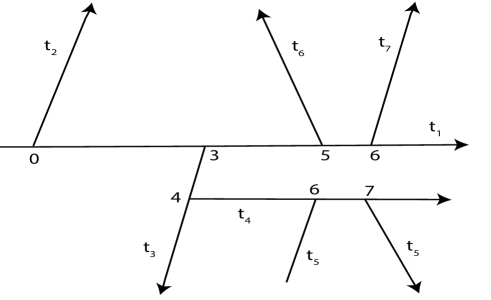
Figure 1: The structure of the manifold ${\cal M}_{\Gamma,I}$ for Example 2.

Definition 2

1. We denote by ${\cal G}$ the set of all ordered sets $G=(G_{1},..,G_{m})$, where $G_{d}\in{\,\!\cal I}$, $d=1,...,m$. We denote by $\bar{\cal G}$ the set of all ordered sets $G=(G_{1},...,G_{m})$, where either $G_{d}=\emptyset$ or $G_{d}\in{\,\!\cal I}$, $d=1,...,m$.

2. For $G\in\bar{\cal G}$, we denote by ${\cal L}^{G}_{2,{\cal T}}$ the set of all ${\cal T}$-branched processes $\{x_{d}\}_{d=1}^{m}$ from ${\cal L}_{2,{\cal T}}$ such that $X_{d}\left(i\omega\right)=0$ for $\omega\in G_{d}$, where $X_{d}={\cal F}x_{d}$.

One may refer $G_{d}$ as the spectrum gaps of $x_{d}$.

Proposition 1

For $\bar{I}\in{\,\!\cal I}$ and $\bar{G}\in{\,\!\cal I}$, let ${\cal U}_{\bar{I},\bar{G}}$ be the set of all $x\in L_{2}({\bf R})$ such that $X\left(i\omega\right)=0$ for $\omega\in\bar{G}$, where $X={\cal F}x$. Let ${\rm mes\,\!}(\bar{I}\cup\bar{G})=+\infty$. Then any $x\in U_{\bar{I},\bar{G}}$ is uniquely defined by its path $x|_{\bar{I}}$.

Corollary 1

Let ${\cal T}=(\Gamma,I)\in{\mathfrak{T}}$ and $\{x_{d}\}_{d=1}^{m}\in{\cal L}^{G}_{2,{\cal T}}$, where $G=(G_{1},...,G_{m})\in{\cal G}$. Let $\{d,k\}\in\Gamma$ and $G_{d}\in{\,\!\cal I}$, $G_{k}\in{\,\!\cal I}$.

1. If ${\rm mes\,\!}(I_{d,k}\cup G_{k})=+\infty$, then $x_{k}$ is uniquely defined by the path $h_{d,k}(x_{d})|_{I_{d,k}}$.

2. If $I_{d,k}\in{\,\!\cal I}_{\infty}$ and ${\rm mes\,\!}(G_{d}\cap G_{k})>0$, then $x_{k}\equiv h_{d,k}(x_{d})$.

3. If ${\rm mes\,\!}(G_{d}\cap G_{k})=+\infty$, then $x_{k}\equiv h_{d,k}(x_{d})$.

Definition 3

Let ${\cal T}=(\Gamma,I,h)\in{\mathfrak{T}}$. Let $d_{0},d\in\{1,...,m\}$, $d_{0}\neq d$. We say that $d_{0}\rightharpoonup d$ if there exists a sequence $\{d_{1},...,d_{j}\}\subset\{1,...,m\}$ such that

$$(d_{0},d_{1}),\ (d_{1},d_{2}),\ \cdots,\ (d_{j},d)\in\Gamma,$$

$$I_{d_{0},d_{1}},\ \ I_{d_{1},d_{2}},\ \ \cdots,\ \ I_{d_{j},d}\in I.$$ (1)

It can be noted that if $h_{d,k}(x)=x$ for all $(d,k)\in\Gamma$ then the relation $\rightharpoonup$ is symmetric.

3 Main results

Let us state first some conditions allowing to recover the entire ${\cal T}$-branched process form a single branch.

Lemma 1

Let ${\cal T}$ and $G=(G_{1},...,G_{m})$ be given such that $G_{d}\in{\,\!\cal I}$ for $d\geq 2$. Assume $1\rightharpoonup d$ for any $d\in\{2,...,m\}$ such that (1) holds and such that

$${\rm mes\,\!}(I_{d_{k-1}}\cup G_{d_{k}})=+\infty,k=1,...,j.$$ (2)

(We assume that $1=d_{0}$ and $d=d_{j+1}$ in (1)). Assume that $\{x_{d}\}_{d=1}^{m}\in{\cal L}^{G}_{2,{\cal T}}$. Then

1. $\{x_{d}\}_{d=1}^{m}$ is uniquely defined by $x_{1}$;

2. If $G_{1}\in{\,\!\cal I}$ then $\{x_{d}\}_{d=1}^{m}$ is uniquely defined by the path $x_{1}|_{\bar{I}}$, for any $\bar{I}\in{\,\!\cal I}_{\infty}$;

3. If $G_{1}\in{\,\!\cal I}_{\infty}$ then $\{x_{d}\}_{d=1}^{m}$ is uniquely defined by the path $x_{1}|_{\bar{I}}$, for any $\bar{I}\in{\,\!\cal I}$.

We say that a ${\cal T}$-branched process $\{x_{d}\}_{d=1}^{m}$ such as described in Lemma 1 features branched spectrum degeneracy with the parameter $({\cal T},G)$.

It can be clarified that, in Lemma 1, the components $x_{d}$ are defined uniquely in $L_{2}({\bf R})$. However, for a ${\cal T}$-branched process from ${\bf C}_{{\cal T}}$, the components $x_{d}$ are defined uniquely in $C({\bf R})$.

Remark 1

It can be noted that the degeneracy required in Lemma 1 can be arbitrarily small, i.e., ${\rm mes\,\!}(G_{d_{k}})$ can be arbitrarily small under assumption (2) given that $I_{d,k}\in{\,\!\cal I}_{\infty}$.

Remark 2

Lemma 1 claims an uniqueness result but does not suggest a method of extrapolation from the set from ${\,\!\cal I}$. Some linear predictors allowing the required extrapolation can be found in [D17] and [5].

The following corollary represents a modification for processes of the classical sampling theorem (Nyquist-Shannon-Kotelnikov Theorem). This Lemma states that a band-limited function $x\in L_{2}({\bf R})$ is uniquely defined by the sequence $\{x(t_{k})\}_{k\in{\bf Z}}$, where given that $X\left(i\omega\right)=0$ for $\omega\notin(-\Omega,\Omega)$ and $X={\cal F}x$, $t_{k}=\tau k$; this theorem allows $\tau\in(0,\leq\pi/\Omega]$. There is a version of this theorem for oversampling sequences with $\tau\in(0,\pi/\Omega)$: for any $s\in{\bf Z}$, this $x$ is uniquely defined by the sequence $\{x(t_{k})\}_{k\in{\bf Z},k\leq s}$ F91 [12, 28]. Corollary 2 below extends this version on the sampling Lemma in the case of ${\cal T}$-branched processes.

Corollary 2

Let the assumptions of Lemma 1 be satisfied, let $\Omega>0$ and $\tau\in(0,\pi/\Omega)$ be given, and let $G_{1}={\bf R}\setminus[-\Omega,\Omega]$ (i.e., the process $x_{1}$ is band-limited). Then, for any $s\in{\bf Z}$, the ${\cal T}$-branched process $\{x_{d}\}_{d=1}^{m}$ is uniquely defined (up to equivalency) by the sampling sequence $\{x_{1}(t_{k})\}_{k\in{\bf Z},\ k\leq s}$, where $t_{k}=\tau k$.

Remark 3

For $k>1$, the processes $x_{k}$ in Corollary 2 are not necessarily band-limited. Moreover, the sampling rate $\tau$ here does not depend on the size of spectrum gaps $G_{k}$ of branches $x_{k}$ for $k\geq 2$. This sampling rate depends only on the size of spectrum support for the single component $x_{1}$.

To proceed further, we introduce some additional conditions for sets ${\cal T}=\{\Gamma,I,H\}\in{\mathfrak{T}}$ restricting choices of $H$.

For $j\in\{1,...,m\}$, let $A(j)\stackrel{{\scriptstyle{\scriptscriptstyle\Delta}}}{{=}}\{k:\ j\rightharpoonup k\}$. For a set $M\subset\{1,...,m\}$, let $A(M)\stackrel{{\scriptstyle{\scriptscriptstyle\Delta}}}{{=}}\cup_{j\in M}A(j)$.

Staring from now, we assume that at least one of the following two conditions is satisfied.

Condition 1

For any $(d,k)\in\Gamma$, the operator $h_{d,k}$ is the identity, i.e. $h_{dk}(x)=x$.

Condition 2

There exists $n\in\{2,...,m\}$, mutually disjoint subsets $M_{p}\subset\{2,...,m\}$, $p=1,...,n$, and an open set $D\subset{\bf R}$ of a positive measure such that the following holds.

1. $1\rightharpoonup d$ for all $d\in M_{p}$ for all $p=1,...,n$;

2. The sets $A(M_{p})$ are mutually disjoint for $p=1,...,n$.

3. If $(d,k)\in\Gamma$ and $d\in A(M_{p})$ for some $p$, then $k\in A(M_{p})$.

4. If $(d,k)\in\Gamma$, then either $k\in\cup_{p=1}^{n}M_{p}$ or $k\in\cup_{p=1}^{n}A(M_{p})$.

5. $h_{d,k}(x)=x$ for all $(d,k)\in\Gamma$ such that either $d\neq 1$ or $d=1$ and $k\notin M_{p}$.

6. For any $p=1,...,n$, there exists an operator ${\rm h}_{p}:L_{2}({\bf R})\to L_{2}({\bf R})$ such that

   (a) $h_{1,k}(x)={\rm h}_{p}(x)$ for all $k\in M_{p}$;

   (b) ${\cal F}({\rm h}_{p}x)={\rm H}_{p}(i\omega)X(i\omega)$ for $(d,k)\in\Gamma_{p}$, where ${\rm H}_{p}\in L_{\infty}(i{\bf R})$ is such that $\mathop{\rm ess\,\!sup}_{\omega\in D}|{\rm H}_{p}(i\omega)^{-1}|<+\infty$.

In particular, Condition 2 (vi)(b) holds if $({\rm h}_{p}x)(t)=ax(bt+c)$ for some $a,b,c\in{\bf R}$, $b\neq 0$, or if $({\rm h}_{p}x)(t)=\int_{\bf R}h(t-s)x(s)ds$, for some $h\in L_{2}({\bf R})$.

Example 3

The set ${\cal T}$ in Example 2 satisfies Condition 2 with

$$M_{1}=\{2\},\quad M_{2}=\{3\},\quad M_{3}=\{6,7\},\quad A(M_{1})=\emptyset,\quad A(M_{2})=\{4,5\},\quad A(M_{3})=\emptyset.$$

Example 4

Consider processes defined in the time domain structured with a closed loop that have just two branches $x_{1}$ and $x_{2}$. These branches are connected via restrictions that $x_{1}(t)=x_{2}(t)$ for $t<0$, and $x_{1}(t)=x_{2}(t-1)$ for $t>1$. These processes can be represented as ${\cal T}$-branched processes $\{x_{d}(t)\}_{d=1}^{2}$ with ${\cal T}=(\{(1,2),\},I,h)$, where $I_{1,2}=(-\infty,0)\cup(1,+\infty)$, and with operator $h_{1,2}:L_{2}({\bf R})\to{\bf R}$ defined so that $(h_{1,2}x)(t)=x(t)$ for $t<0$, and $(h_{1,2}x)(t)=x(1-t)$ for $t\geq 0$. This ${\cal T}$ does not satisfy Conditions 1 and 2 since the operator $h$ does not satisfy Condition 2 (vi)(b).

Example 5

Technically, Example 4 can be modified so that the same restrictions for $x_{1}$ and $x_{2}$ hold but the operator $h$ satisfy Condition 2 (vi)(b). This can be achieved by adding a dummy branch. More precisely, consider a ${\cal T}$-branched process $\{x_{d}(t)\}_{d=1}^{3}$ with ${\cal T}=(\{(1,2),(3,1),(2,3)\},I,h)$, where

$$I_{1,2}=I_{3,1}=(-\infty,0),\quad I_{2,3}=(0,+\infty),\quad h_{1,2}x=h_{3,1}x\equiv x,\quad(h_{3,2}x)(t)=x(1-t).$$

Here $x_{3}$ is a dummy branch supplementing the process from Example 4. This corresponds to restrictions $x_{1}(t)=x_{2}(t)$ for $t<0$, $x_{1}(t)=x_{3}(t)$ for $t<0$, $x_{2}(t)=x_{3}(1-t)$ for $t>1$. With this modification, Condition 2(vi) for $h$ is satisfied. However, Condition2 on $(\Gamma,I)$ is not satisfied.

Lemma 2

Let ${\cal T}=(\Gamma,I,h)\in{\mathfrak{T}}$ be such that either Condition 1 or Condition 2 holds. Then the following holds.

1. For any ${\cal T}$-branched process $\{x_{d}\}_{d=1}^{m}\in{\cal L}_{2,{\cal T}}$, and for any $\varepsilon>0$, there exists $G\in{\cal G}$ and a ${\cal T}$-branched process $\{\widehat{x}_{d}\}_{d=1}^{m}\in{\cal L}^{G}_{2,{\cal T}}$ such that

   $$\max_{d=1,...,m}\|x_{d}-\widehat{x}_{d}\|_{L_{2}({\bf R})}\leq\varepsilon.$$ (5)

2. For any branching ${\cal T}$-branched process $\{x_{d}\}_{d=1}^{m}\in{\cal C}_{{\cal T}}$ and any $\varepsilon>0$, there exists $G\in{\cal G}$ and a ${\cal T}$-branched process $\{\widehat{x}_{d}\}_{d=1}^{m}\in{\cal L}_{2,{\cal T}}^{G}\cap{\cal C}_{{\cal T}}$ such that

   $$\max_{d=1,...,m}(\|x_{d}-\widehat{x}_{d}\|_{L_{2}({\bf R})}+\|x_{d}-\widehat{x}_{d}\|_{C({\bf R})})\leq\varepsilon.$$ (6)

3. Let $\bar{G}_{1}\in{\,\!\cal I}$ be given such that ${\rm mes\,\!}(D\setminus\bar{G}_{1})>0$, where $D$ is the set in Condition 2. Let $x_{1}$ be such that $X_{1}(i\omega)|_{\omega\in\bar{G}_{1}}=0$ for $X_{1}={\cal F}x_{1}$. In this case, $G=(G_{1},...,G_{m})$ in statements (i) and (ii) above can be selected so that $G_{1}=\bar{G}_{1}$.

It should be emphasized that Lemma 2 claims existence of processes $\{x_{d}\}$ featuring preselected spectrum degeneracy for the branches and, at the same time, such that the branches coinciding on preselected intervals. This cannot be achieved by a simple application of low/high pass filters to separate branches; if one applies such filters to $x_{d}$ and $x_{k}$, this will impact the values on $I_{k,d}$, and the identity $x_{k}|_{I_{d,k}}=h_{d,k}(x_{d})|_{I_{d,k}}$ could be disrupted.

Lemma 2 combined with Lemma 1 allows to approximate a ${\cal T}$-branched process by a process that can be recovered from a single branch. However, condition (2) in Lemma 1 and Conditions 1-2 restrict choices of ${\cal T}$ and $G$ where this approximation is feasible. Nevertheless, there are choices of topology ${\cal T}$ satisfying these conditions.

The following result provides sufficient conditions that ensure that a ${\cal T}$-branched process can be recovered from its branch.

Theorem 1

Assume that ${\cal T}=\{\Gamma,I,H\}\in{\mathfrak{T}}$ is such that either Condition 1 or Condition 2 holds, and that $I_{d,k}\in{\,\!\cal I}_{\infty}$ for all $\{d,k\}\in\Gamma$. Then the following holds.

1. For any ${\cal T}$-branched process $\{x_{d}\}_{d=1}^{m}\in{\cal L}_{2,{\cal T}}$ there exists $G\in{\cal G}$ and a ${\cal T}$-branched process $\{\widehat{x}_{d}\}_{d=1}^{m}\in{\cal L}_{2,{\cal T}}^{G}$ satisfying the assumptions of Lemma 1 and such that (5) holds.

2. For any ${\cal T}$-branched process $\{x_{d}\}_{d=1}^{m}\in{\cal C}_{{\cal T}}$ there exists $G\in{\cal G}$ and a ${\cal T}$-branched process $\{\widehat{x}_{d}\}_{d=1}^{m}\in{\cal L}_{{\cal T}}^{G}\cap{\cal C}_{{\cal T}}$ satisfying the assumptions of Lemma 1 and such that (6) hold.

The processes $\{\widehat{x}_{d}\}_{d=1}^{m}\in{\cal L}_{2,{\cal T}}^{G}$ are uniquely defined by their path $\widehat{x}_{1}|_{\bar{I}}$, for any $\bar{I}\in{\,\!\cal I}_{\infty}$. Under the assumptions of Lemma 2(iii) with $\bar{G}=G_{1}\in{\,\!\cal I}_{\infty}$, the processes $\{\widehat{x}_{d}\}_{d=1}^{m}$ are uniquely defined by the path $\widehat{x}_{1}|_{\bar{I}}$ for any $\bar{I}\in{\,\!\cal I}$.

It can be noted that, under the assumptions of Theorem 1, by Corollary 1, the spectrum gaps for different branch processes $x_{d}$ should be disjoint; otherwise, the branches coincide, and it would makes some branches redundant in the model. This reduces choices of topological structures for processes that can be recovered from a singe branch, since the processes with compact spectrum gap can be recovered uniquely from semi-infinite intervals of observations only. However, there is an important example that satisfy these restrictions such as examples listed below.

Example 6

Consider ${\cal T}=(\{(1,d)\}_{d=1}^{m},I,h)$, where $I_{1,d}=(-\infty,0)\cup(1,+\infty)$, and where $h$ is any operator satisfying Condition 2. This ${\cal T}$ satisfy the assumptions of Theorem 1.

Example 7

Consider ${\cal T}=(\{(1,d)\}_{d=1}^{m},I,h)$, where $I_{1,d}=(-\infty,0)\cup(1,+\infty)$, i.e., with $x_{1}(t)=x_{d}(t)$ for $t\notin[0,1]$ for all $d$ for ${\cal T}$-branched processes. This process satisfy the assumptions of Theorem 1.

Example 8

${\cal T}$ from Example 2 satisfy the assumptions of Theorem 1 given that ${\rm mes\,\!}(G_{5})=+\infty$. On the other hand, the sets ${\cal T}$ from Examples 4-5 do not satisfy any of Conditions 1 and 2, and, respectively, they do not satisfy the assumptions of Theorem 1.

4 Applications: sampling theorem for branching processes

Theorem 2

Let the assumptions of Theorem 1(ii) hold, let $\Omega>0$ and $\tau\in(0,\pi/\Omega)$ be given. Consider a ${\cal T}$-branched process $\{\widetilde{x}_{d}\}_{d=1}^{m}\in{\cal L}_{2,{\cal T}}^{G}$ such that $X_{1}(i\omega)=0$ if $|\omega|>\Omega$ for $X={\cal F}x$ (i.e., the process $x_{1}$ is band-limited). Then, for any $\varepsilon>0$, there exists $G\in{\cal G}$ and ${\cal T}$-branched process $\{\widetilde{x}_{d}\}_{d=1}^{m}\in{\cal L}_{2,{\cal T}}^{G}\cap{\cal C}_{\cal T}$ such that $G_{1}={\bf R}\setminus[-\Omega,\Omega]$, that (5) holds, and that the following holds:

1. the ${\cal T}$-branched process $\{\widetilde{x}_{d}\}_{d=1}^{m}\in{\cal L}_{2,{\cal T}}^{G}$ is uniquely defined (up to equivalency) by the sampling sequence $\{x_{d}(t_{k})\}_{k\in{\bf Z},d=1,..,m}$, where $t_{k}=\tau k$.

2. Moreover, for any $s\in{\bf Z}$, the ${\cal T}$-branched process $\{\widetilde{x}_{d}\}_{d=1}^{m}\in{\cal L}_{2,{\cal T}}^{G}$ is uniquely defined (up to equivalency) by the sampling sequence $\{x_{1}(t_{k})\}_{k\in{\bf Z},\ k\leq s}$, where $t_{k}=\tau k$.

The conditions of Theorem 2 restrict choices of branched processes. However, they still hold for many models describing branching scenarios.

Example 9

Let $x_{1}(t)$ be a coordinate of a fighter jet tracked by a locator for time $t<0$, and let this jet ejects $m-1$ false targets at time $t=0$; these false targets move according to different evolution laws. This can be modelled by a ${\cal T}$-branched process $\{x_{d}\}_{d=1}^{m}$ with a ${\cal T}=(\{(1,d)\}_{d=2}^{m},I,h)$, where $I_{1,d}=(-\infty,0)$, and where $h_{1,d}(x)\equiv x$, i.e. with $x_{1}(t)=x_{d}(t)$ for $t<0$ for all $d$. It is not obvious how to apply the approach of the classical sampling theorem in this situation. On the other hand, this case is covered by Theorem 2. Therefore, for any $\varepsilon>0$, there exist a ${\cal T}$-branched process $\{\widehat{x}_{d,\varepsilon}\}_{k=1}^{m}$, such that the following holds:

1. $\sup_{t\in{\bf R}}|\widehat{x}_{1,\varepsilon}(t)-x_{1}(t)|\leq\varepsilon$,  $\sup_{t>0}|\widehat{x}_{d,\varepsilon}(t)-x_{d}(t)|\leq\varepsilon$;

2. For any $\tau\in(0,\pi/\Omega)$ and $s<0$, an equidistant sequence $\{\widehat{x}_{\varepsilon,1}(\tau k)\}_{k\in{\bf Z},\ k<s}$ defines $\{\widehat{x}_{d,\varepsilon}(\cdot)\}_{d=1}^{m}$ uniquely.

5 Proofs

Proof of Proposition 1. The statements of this proposition are known; for completeness, we provide the proof.

Cleary, ${\rm mes\,\!}(\bar{I}\cup\bar{G})=\infty$ if and only if either $\bar{I}\in{\,\!\cal I}_{\infty}$ or $\bar{G}\in{\,\!\cal I}_{\infty}$. Let us consider the case where $\bar{I}\in{\,\!\cal I}_{\infty}$. Without loss of generality, we assume that $(-\infty,0)\subset\bar{I}$. Let ${\bf C}^{+}\stackrel{{\scriptstyle{\scriptscriptstyle\Delta}}}{{=}}\{z\in{\bf C}:\ {\rm Re\,\!}z>0\}$, and let $H^{2}$ be the Hardy space of holomorphic on ${\bf C}^{+}$ functions $h(p)$ with finite norm $\|h\|_{H^{2}}=\sup_{s>0}\|h(s+i\omega)\|_{L_{2}({\bf R})}$; see, e.g. [10], Chapter 11. It suffices to prove that if $x\in L_{2}({\bf R})$ is such that $X\left(i\omega\right)=0$ for $\omega\in\bar{G}$, $X={\cal F}x$, and $x(t)=0$ for $t\leq 0$, then $x(t)=0$ for $t>0$. These properties imply that $X\in H^{2}$, and, at the same time,

$$\int_{-\infty}^{+\infty}(1+\omega^{2})^{-1}|\log|X\left(i\omega\right)||dx=+\infty.$$

Hence, by the property of the Hardy space, $X\equiv 0$; see, e.g. Lemma 11.6 in [10], p. 193. This proves the statement of Proposition 1 for the case where $\bar{I}\in{\,\!\cal I}_{\infty}$. Because of the duality between processes in time domain and their Fourier transforms, this also implies the proof for the case where $\bar{G}\in{\,\!\cal I}_{\infty}$. This completes the proof of Proposition 1. $\Box$

Proof of Corollary 1 follows immediately from the definitions and from Proposition 1. $\Box$

Proof of Lemma 1. Let $\bar{I}\in{\,\!\cal I}$ be such that $\bar{I}={\bf R}$ for statement (i), $I\in I_{\infty}$ for statement (ii), $I\in{\,\!\cal I}$ for statement (iii).

By Proposition 1, $x_{1}$ is uniquely defined by $x_{1}|_{\bar{I}}$. Further, let $N=d_{N}\in\{2,3,...,m\}$ be given. By Lemma 1, $x_{d_{1}}$ is uniquely defined by $h_{d_{1},d_{0}}(x_{1})|_{I_{d_{0},d_{1}}}$, i.e., by $x_{1}|_{\bar{I}}$. Similarly, $x_{d_{2}}$ is uniquely defined by $x_{d_{2}}|_{I_{d_{2},d_{1}}}=h_{d_{1},d_{2}}(x_{d_{1}})|_{I_{d_{2},d_{1}}}$, i.e., by $x_{1}|_{\bar{I}}$ again. Repeating this for all $d_{k}$, $k=1,...,j$, we obtain that $x_{d_{j}}$ is uniquely defined by $x_{1}|_{\bar{I}}$. Hence $x_{d}$ is uniquely defined by $x_{1}|_{\bar{I}}$. This completes the proof of Lemma 1. $\Box$

Proof of Corollary 2. It follows from the results F91 [12, 28] that $x_{1}$ is uniquely defined by $\{x_{1}(t_{k})\}_{k\leq s}$. Then the statement of Corollary 2 follows from Lemma 1. $\Box$

Proof of Lemma 2. Let us suggest a procedure for the construction of $\widehat{x}$; this will be sufficient to prove the theorem. This procedure is given below.

Let us assume first that Condition 2 holds.

For $(d,k)\in\Gamma$, let $H_{kd}(i\omega)=1$ if either $d\neq 1$ or $k\notin\cup_{p=1}^{n}M_{p}$, and where $H_{1k}(i\omega)={\rm H}_{p}(i\omega)$ if $k\in M_{p}$.

Let

$$y_{k,d}\stackrel{{\scriptstyle{\scriptscriptstyle\Delta}}}{{=}}x_{k}-h_{dk}(x_{d}),\quad Y_{k,d}\stackrel{{\scriptstyle{\scriptscriptstyle\Delta}}}{{=}}{\cal F}y_{k,d}=X_{k}-h_{kd}X_{d},$$

where $X_{k}\stackrel{{\scriptstyle{\scriptscriptstyle\Delta}}}{{=}}{\cal F}x_{k}$.

Consider a set $\{\omega_{k}\}_{k=1,...,m}\subset{\bf R}$ such that $\omega_{k}$ are located in the interior $D\setminus\bar{G}_{1}$ for $k\geq 2$. Let $G_{k}=J_{k}(\delta)$. Here $J_{k}(\delta)\stackrel{{\scriptstyle{\scriptscriptstyle\Delta}}}{{=}}(\omega_{k}-\delta,\omega_{k}+\delta)$ for $k>1$, $J_{1}(\delta)\stackrel{{\scriptstyle{\scriptscriptstyle\Delta}}}{{=}}(\omega_{1}-\delta,\omega_{1}+\delta)$ if $G_{1}$ has to be selected, and $J_{1}(\delta)\stackrel{{\scriptstyle{\scriptscriptstyle\Delta}}}{{=}}\bar{G}_{1}$ if $G_{1}=\bar{G}_{1}$ is fixed (i.e., in the case of Lemma 2(iii)).

We assume below that $\delta>0$ is small enough such that these intervals are disjoint and that $J_{k}(\delta)\subset D$ for $k\geq 2$; this choice of $\delta$ is possible since $\omega_{k}\neq\omega_{j}$ if $j\neq k$.

Let $M^{c}\stackrel{{\scriptstyle{\scriptscriptstyle\Delta}}}{{=}}\{k=2,...,m\}\setminus(\cup_{p=1}^{n}M_{p})$ and $B\stackrel{{\scriptstyle{\scriptscriptstyle\Delta}}}{{=}}M^{c}\cup(\cup_{p=1}^{n}A(M_{p}))$. Set

$$\widehat{X}_{1}\left(i\omega\right)\stackrel{{\scriptstyle{\scriptscriptstyle\Delta}}}{{=}}X_{1}\left(i\omega\right){\mathbb{I}}_{\{\omega\notin\cup_{d=1}^{m}J_{d}(\delta)\}}-\sum_{d\in B}Y_{d,1}\left(i\omega\right){\mathbb{I}}_{\{\omega\in J_{d}(\delta)\}}$$

$$-\sum_{p=1}^{n}{\rm H}_{p}(i\omega)^{-1}\sum_{d\in M_{p}}Y_{d,1}\left(i\omega\right){\mathbb{I}}_{\{\omega\in J_{d}(\delta)\}}$$

and

$$\widehat{X}_{d}\stackrel{{\scriptstyle{\scriptscriptstyle\Delta}}}{{=}}H_{1,d}\widehat{X}_{1}+Y_{d,1},\quad d=2,...,m.$$

For $k\in M_{p}\cup A(M_{p})$ and $d\in A(M_{p})$, we have that

$$\widehat{X}_{k}-H_{d,k}\widehat{X}_{d}=\widehat{X}_{k}-\widehat{X}_{d}=\widehat{X}_{1}+Y_{k,1}-\widehat{X}_{1}-Y_{d,1}=Y_{k,1}-Y_{d,1}=X_{k}-X_{1}-X_{d}+X_{1}=Y_{k,d},$$

i.e.

$$\widehat{X}_{k}=\widehat{X}_{d}+Y_{k,d}.$$

Let $\widehat{x}_{d}={\cal F}^{-1}\widehat{X}_{d}$, $d=1,...,m$.

Under the assumptions of statement (i) of the theorem, we have that $x_{k}|_{I_{d,k}}=H_{d,k}(x_{d})|_{I_{d,k}}$ up to equivalency. It follows that $y_{k,d}|_{I_{d,k}}=0$ up to equivalency, i.e. $\widehat{x}_{k}|_{I_{d,k}}=h_{d,k}(\widehat{x}_{d})|_{I_{d,k}}$ up to equivalency. Since this holds for all $(d,k)\in\Gamma$, it follows that $\{\widehat{x}_{d}\}_{d=1}^{m}$ is a ${\cal T}$-branched process with the same structure set ${\cal T}$ as the underlying ${\cal T}$-branched process $\{x_{d}\}_{d=1}^{m}$.

Let us show that the ${\cal T}$-branched process $\{\widehat{x}_{d}\}_{d=1}^{m}$ features the required spectrum degeneracy.

Since the intervals $J_{d}(\delta)$ are mutually disjoint, it follows immediately from the definition for $\widehat{X}_{1}$ that $\widehat{X}_{1}\left(i\omega\right)=0$ for $\omega\in J_{1}(\delta)$.

Further, by the definition for $\widehat{X}_{d}$ for $d>1$, we have that

$$\widehat{X}_{d}\left(i\omega\right)=H_{1,d}\Bigl{(}X_{1}\left(i\omega\right){\mathbb{I}}_{\{\omega\notin\cup_{d=1}^{m}J_{d}(\delta)\}}-\sum_{d\in B}Y_{d,1}\left(i\omega\right){\mathbb{I}}_{\{\omega\in J_{d}(\delta)\}}$$

$$-\sum_{p=1}^{n}{\rm H}_{p}(i\omega)^{-1}\sum_{d\in M_{p}}Y_{d,1}\left(i\omega\right){\mathbb{I}}_{\{\omega\in J_{d}(\delta)\}}\Bigr{)}+Y_{d,1}\left(i\omega\right).$$

Since the intervals $G_{d}=J_{d}(\delta)$ are mutually disjoint, we have that

$$\widehat{X}_{d}\left(i\omega\right){\mathbb{I}}_{\{\omega\in J_{d}(\delta)\}}=0-Y_{d,1}\left(i\omega\right){\mathbb{I}}_{\{\omega\in J_{d}(\delta)\}}+Y_{d,1}{\mathbb{I}}_{\{\omega\in J_{d}(\delta)\}}=0.$$

We obtain that separately for $d\in B$ and $d\notin B$, using properties of ${\rm H}_{p}$, $H_{1,d}$ implied from their definitions.

It follows that $\widehat{X}_{d}\left(i\omega\right)=0$ for $\omega\in J_{d}(\delta)$ for $d>1$ as well. It follows that the ${\cal T}$-branched process $\{\widehat{x}_{d}\}_{d=1}^{m}$ belongs to ${\cal L}_{2,{\cal T}}^{G}$ with $G_{d}=J_{\delta}(d)$, i.e. features the required spectrum degeneracy.

Furthermore, for all $d$, we have that, under the assumptions of statement (i), $\|X_{d}(i\cdot)-\widehat{X}_{d}(i\cdot)\|_{L_{2}({\bf R})}\to 0$ as $\delta\to 0$. In addition, we have that, under the assumptions of statement (ii),

$$\|X_{d}(i\cdot)-\widehat{X}_{d}(i\cdot)\|_{L_{2}({\bf R})}+\|X_{d}(i\cdot)-\widehat{X}_{d}(i\cdot)\|_{L_{1}({\bf R})}\to 0$$

as $\delta\to 0$. Under the assumptions of statement (i), it follows that $\|\widehat{x}_{d}-x_{d}\|_{L_{2}({\bf R})}\to 0$. Under the assumptions of statement (ii), it follows that $\|\widehat{x}_{d}-x_{d}\|_{L_{2}({\bf R})}+\|\widehat{x}_{d}-x_{d}\|_{L_{2}({\bf R})}\to 0$ as $\delta\to 0$.

For the proof under Condition 1, we select

$$\widehat{X}_{1}\left(i\omega\right)\stackrel{{\scriptstyle{\scriptscriptstyle\Delta}}}{{=}}X_{1}\left(i\omega\right){\mathbb{I}}_{\{\omega\notin\cup_{d=1}^{m}J_{d}(\delta)\}}-\sum_{d=2}^{m}Y_{d,1}\left(i\omega\right){\mathbb{I}}_{\{\omega\in J_{d}(\delta)\}}.$$

Then the proof is similar to the proof for the case where Condition 2 holds. This completes the proof of Lemma 2. $\Box$

It can be noted that the construction in the proof of Lemma 2 follows the approach suggested in [9] for discrete time processes. Let us illustrate the construction using a toy example.

Example 10

Let $m=2$, and ${\cal T}=(\Gamma,I,h)$ be such that $\Gamma=\{(1,2)\}$, $I_{1,2}(x)=(-\infty,0)\cup(1,+\infty)$, $h_{1,2}(x)=x$. This choice imposes restrictions $x_{1}(t)=x_{2}(t)$ for $t\notin[0,1]$.

Further, in the notations of the proof of Lemma 2(iii), let $\bar{G}_{1}=\{\omega\in{\bf R}:\ |\omega|>1\}$, $\omega_{2}=0$, $x_{1}(t)\equiv 0$, and $x_{2}(t)={\mathbb{I}}_{[0,1]}$. In this case, we have that

$$X_{1}(i\omega)=0,\quad X_{2}(i\omega)=\frac{1-e^{-i\omega}}{i\omega},\quad Y_{2,1}(i\omega)=X_{2}(i\omega).$$

Let us select $J_{1}(\delta)=\bar{G}_{1}$ and $J_{2}(\delta)=\{\omega:\ |\omega|\leq\delta\}$, $\delta\in(0,1)$. The corresponding processes $\widehat{X}_{d}$ are

$$\widehat{X}_{1}(i\omega)=0-Y_{2}(i\omega){\mathbb{I}}_{\{|\omega|\leq\delta\}}=-X_{2}(i\omega){\mathbb{I}}_{\{|\omega|\leq\delta\}},\quad\widehat{X}_{2}(i\omega)=\widehat{X}_{1}+Y_{2,1}=X_{2}(i\omega){\mathbb{I}}_{\{|\omega|>\delta\}}.$$

This gives

$$\widehat{x}_{1}(t)=\frac{1}{2\pi}\int_{-\delta}^{\delta}e^{i\omega}\frac{1-e^{-i\omega}}{i\omega}d\omega,\widehat{x}_{2}(t)=x_{2}(t)+\widetilde{x}_{1}(t).$$

Clearly, $\widehat{x}_{1}(t)=\widehat{x}_{2}(t)$ for $t\notin[0,1]$. Hence $\{\widehat{x}_{d}\}_{d=1,2}\in{\cal L}_{2,{\cal T}}^{G}$ is a ${\cal T}$-branched process with $G=(\bar{G}_{1},G_{2})$ and $G_{2}=\{\omega\in{\bf R}:\ |\omega|\leq\delta\}$. For sufficiently small $\delta$, the processes $\widehat{x}_{d}$ can be arbitrarily close to $x_{d}$. The process $\widehat{x}_{2}$ has a spectrum gap $J_{2}(\delta)$ and can be recovered [5] from its path $\widehat{x}_{2}|_{t<0}=\widehat{x}_{1}|_{t<0}$; this recovery is uniquely defined in the class of processes featuring this spectrum gap. The process $\widehat{x}_{1}$ is band-limited and can be recovered from its semi-infinite sample as described in Corollary 2; this recovery is uniquely defined in the class of band-limited processes with the same spectrum band.

Proof of Theorems 1 and 2 follows immediately from Lemmas 1–2. $\Box$

6 Conclusions and future research

The present paper is focused on the frequency analysis for processes with time domain represented as oriented branched 1-manifolds that can be considered as an oriented graph with continuous connected branches. The paper suggests an approach that allows to take into account the topology of the branching line via modelling it as a system of standard processes defined on the real axis and coinciding on preselected intervals with well-defined Fourier transforms (Definition 1). This approach allows a relatively simple and convenient representation of processes defined on time domains represented as a 1-manifold, including manifolds represented by restrictions such as $x_{k}(t)=x_{d}(t+\tau)$ or $x_{k}(t)=x_{d}(\tau-t)+c$, or $x_{k}(t)=\int_{\bf R}h(t-s)x_{d}(s)ds$, for $t\in I$, with arbitrarily chosen preselected $I_{d,k}\subset{\bf R}$, $c,\tau\in{\bf R}$, and $h\in L_{2}({\bf R})$.

It could be interesting to extend the results on processes with time domain represented as compact oriented branched 1-manifolds. Possibly, it can be achieved via extension of the domain of these processes. For example, one could extend edges of compact branching line beyond their vertices and transform finite edges into semi-infinite ones. Alternatively, one could supplement the branching lines by new dummy semi-infinite edges originated from the vertices of order one. We leave them for the future research.

In addition, Lemma 1 and Theorem 1 can be extended on the case of processes $\widetilde{x}_{d}$ with the spectrum vanishing at single points with sufficiently high vanishing rate such as described in [6].

References

- [1] Anis, A., Gadde, A., and Ortega, A. (2016). Efficient sampling set selection for band-limited graph signals using graph spectral proxies. IEEE Trans. Signal Processing 64 (14), 3775-3789.
- [2] Anis, A. El Gamal, A., Ortega, A. (2019) A Sampling theory perspective of graph-based semi-supervised learning. IEEE Transactions on Information Theory 65:4, 2322-2342.
- [3] Chekhov, L.O., N. V. Puzyrnikova, N.V. (2000). Integrable systems on graphs. Russian Math. Surveys 55:5, 992–994
- [4] Chen, S., Varma, R., Sandryhaila, A., and Kovacevic, J. (2015). Discrete signal processing on graphs: Sampling theory. IEEE Trans. Signal Processing 63 (24), 6510-6523.
- [5] Dokuchaev, N. (2008). The predictability of band-limited, high-frequency, and mixed processes in the presence of ideal low-pass filters. Journal of Physics A: Mathematical and Theoretical 41, No 38, 382002. (7pp).
- [6] Dokuchaev, N. (2021). Pathwise continuous time weak predictability and single point spectrum degeneracy. Applied and Computational Harmonic Analysis, (53) 116–131.
- [7] Dokuchaev, N. (2017). Spectrum degeneracy for functions on branching lines and impact on extrapolation and sampling. arXiv:1705.06181.
- [8] Dokuchaev, N. (2018). On causal extrapolation of sequences with applications to forecasting. Applied Mathematics and Computation 328, pp. 276-286.
- [9] Dokuchaev, N. (2019). On recovery of discrete time signals from their periodic subsequences. Signal Processing 162 180-188.
- [10] Duren, P. (1970). Theory of -Spaces. Academic Press, New York.
- [11] Folz,M. Volume growth and stochastic completeness of graphs. (2014). Trans. Amer. Math. Soc. 366, 2089-2119
- [12] Ferreira P. G. S. G. (1992). Incomplete sampling series and the recovery of missing samples from oversampled band-limited signals. IEEE Trans. Signal Processing 40, iss. 1, 225-227.
- [13] Hadeler, K.P. and Hillen, T. (1994). Differential Equations on Branched Manifolds. In: Evolution Equations, Control Theory and Biomathematics, P. Clement and G. Lumer (eds), Han-sur-Lesse, 241–258, Marcel Dekker, 1994.
- [14] Hajri, H., Olivier Raimond, O. Stochastic flows on metric graphs. Electron. J. Probab. 19 (2014), no. 12, 1-20.
- [15] Huang, X. (2012). On uniqueness class for a heat equation on graphs. Journal of Mathematical Analysis and Applications 393 (2), pp.377-388.
- [16] Jung, A,, Hero, A.,O., A. C. Mara, A.C., S. Jahromi, S, A. Heimowitz, A., and Eldar, Y. C. (2019). Semi-Supervised Learning in Network-Structured Data via Total Variation Minimization. IEEE Transactions on Signal Processing, vol. 67, no. 24, 6256-6269.
- [17] Jung, A., N Tran, N., A Mara, A., (2018). When is network lasso accurate?. Frontiers in Applied Mathematics and Statistics. https://doi.org/10.3389/fams.2017.00028.
- [18] Keller, M., and Lenz, D. (2012). Dirichlet forms and stochastic completeness of graphs and subgraphs, J. Reine Angew. Math. 666, 189-223
- [19] Landau H.J. (1967). Sampling, data transmission, and the Nyquist rate. Proc. IEEE 55 (10), 1701-1706.
- [20] Nguyen, H. and Do, M. (2015). Downsampling of signals on graphs via maximum spanning trees, IEEE Transactions on Signal Processing, 63 (1), pp. 182-191.
- [21] Olevski, A., and Ulanovskii, A. (2008). Universal sampling and interpolation of band-limited signals. Geometric and Functional Analysis, vol. 18, no. 3, pp. 1029–1052.
- [22] Olevskii A.M. and Ulanovskii A. (2016). Functions with Disconnected Spectrum: Sampling, Interpolation, Translates. Amer. Math. Soc., Univ. Lect. Ser. Vol. 46.
- [23] Pokorny, Y.V., Penkin, O.M., Pryadier, V.L., Borovskikh, A.V., Lazarev, K.P., and Shabrov, S.A.(2004). Differential Equations on Geometric Graphs. Moscow, FIZMATLIT.
- [24] Post, O. (2012). Spectral Analysis on Graph-Like Spaces, Springer.
- [25] van der Schaft, A. J., Schumacher, J. M. (2000). An Introduction to Hybrid Dynamical Systems. Springer Verlag, London.
- [26] Sandryhaila, A. Moura, J. (2014). Big data analysis with signal processing on graphs: Representation and processing of massive data sets with irregular structure. IEEE Signal Processing Magazine 31, no. 5, pp. 80-90.
- [27] Shuman, D., Narang, S., Frossard, P., Ortega, A., and P. Vandergheynst, P. (2013). The emerging field of signal processing on graphs: Extending high-dimensional data analysis to networks and other irregular domains. IEEE Signal Processing Magazine 30, no. 3, pp. 83–98.
- [28] Vaidyanathan P.P. (1987). On predicting a band-limited signal based on past sample values,” Proceedings of the IEEE 75 (8), pp. 1125–1127.