DeepScaffold: a comprehensive tool for scaffold-based de novo drug discovery using deep learning

Abstract

The ultimate goal of drug design is to find novel compounds with desirable pharmacological properties. Designing molecules retaining particular scaffolds as the core structures of the molecules is one of the efficient ways to obtain potential drug candidates with desirable properties. We proposed a scaffold-based molecular generative model for scaffold-based drug discovery, which performs molecule generation based on a wide spectrum of scaffold definitions, including BM-scaffolds, cyclic skeletons, as well as scaffolds with specifications on side-chain properties. The model can generalize the learned chemical rules of adding atoms and bonds to a given scaffold. Furthermore, the generated compounds were evaluated by molecular docking in DRD2 targets and the results demonstrated that this approach can be effectively applied to solve several drug design problems, including the generation of compounds containing a given scaffold and de novo drug design of potential drug candidates with specific docking scores.

Stonewise, Beijing, China Contributed equally to this work Contributed equally to this work

1 Introduction

"Molecular scaffold" is one of the most important and widely used concepts in medicinal chemistry. Given a chemical compound, its "scaffold" generally represents the core structures of the molecular framework ¹. Although various definitions of molecular scaffolds are available, the most widely adopted version is given by Bemis and Murcko ², who obtain the scaffold by removing all side chains (or R-groups). Among all scaffolds, those with preferable bioactivity properties (which are referred to as "privileged scaffolds"³ or "bioactive scaffolds"^{4, 5}) are of particular interest to drug discovery. Privileged scaffolds are often used as a starting point for compound synthesis or diversification. Previous researches have developed various types of tools to extract and utilize information from scaffolds, including tools for the discovery of privileged scaffolds (such as CSE ⁶ and ⁵), tools for organizing scaffolds (such as HierS ⁷, SCONP ⁸, ST⁹ and SN⁴), as well as tools for visualization (such as Scaffold Hunter ¹⁰).

Recently, deep learning ¹¹ have revealed itself as a new and promising tool for many drug-design-related problems. In particular, there is a growing interest in using deep generative models¹² for de novo molecule design¹³. Early works in this area ^{14, 15, 16} mainly utilizes RNN based architectures (such as GRU ¹⁶ or LSTM ¹⁴) to generate SMILES strings ¹⁷, which is a serialized representation of molecules graph. Those methods have proven to be very effective for de novo molecule design, but still faces certain issues, such as the need to learn SMILES gramma. Recent works ^{18, 19, 20, 21, 22} have improved upon this approach by using graph-based representations of molecules. Also, other types of generative architecture have been explored, such as GAN ²³. Those models have been successfully applied to various drug design problems, such as the property-based design of virtual libraries ^{18, 16}, ligand^{14, 18, 16} and structural²⁴ based drug design, as well as local optimization of molecular structures^{16, 22}.

With the promising performance, it is natural to apply deep generative models to scaffold directed drug design. Early works have used conditional generative model ¹⁸, reinforcement learning ¹⁸ or transfer learning ²⁵ to achieve molecule generation based on scaffold queries. However, those methods do not guarantee that the outputs molecule will match the input query, and are difficult to be extended to new scaffolds. A recent publication by Lim et. al. ²⁶ solved the problems above using a model that directly grow molecules on the given scaffold. However, the model is restricted only to BM-scaffolds, which does not necessarily fit well with all tasks in medicinal chemistry.

In this work, we introduce DeepScaffold, a novel and comprehensive solution for scaffold-based drug discovery. Different from previous methods, DeepScaffold can perform molecule generation based on a wide spectrum of scaffold definitions, including BM-scaffolds, cyclic skeletons, as well as scaffolds with specifications on side-chain properties. Our proposed method can guarantee that the output molecule would match the scaffold query, and can be easily extended to new scaffolds outside the training set. A broad set of evaluation is carried out to access the performance of DeepScaffold. We also discuss several challenges faced when evaluating such scaffold-based generative models.

2 Methods

Figure 1: An overview of DeepScaffold. DeepScaffold is a comprehensive tool for scaffold-directed drug discovery, capable of performing molecule generation based on a. cyclic skeletons (CSKs), b. classical molecular scaffolds, such as Bemis-Murko scaffolds, as well as c. scaffolds with additional pharmacophore-based queries for side chains.

2.1 An overview of DeepScaffold

Before diving into the implementation details, we first take a look at the overall architecture of DeepScaffold. As mentioned earlier, DeepScaffold is capable of performing de novo drug design based on the following scaffold definitions (Figure1):

• Cyclic skeletons

• Scaffolds with atom and bond type information, such as Bemis-Murko scaffold

• Scaffolds with additional specification on side-chain properties

Figure 2: The basic components for DeepScaffold. As shown in the figure, DeepScaffold is composed of the following three models: a. A neural network for completing atom and bond type for cyclic skeletons; b. A scaffold-based molecule generative model; c. A filter based on side-chain properties

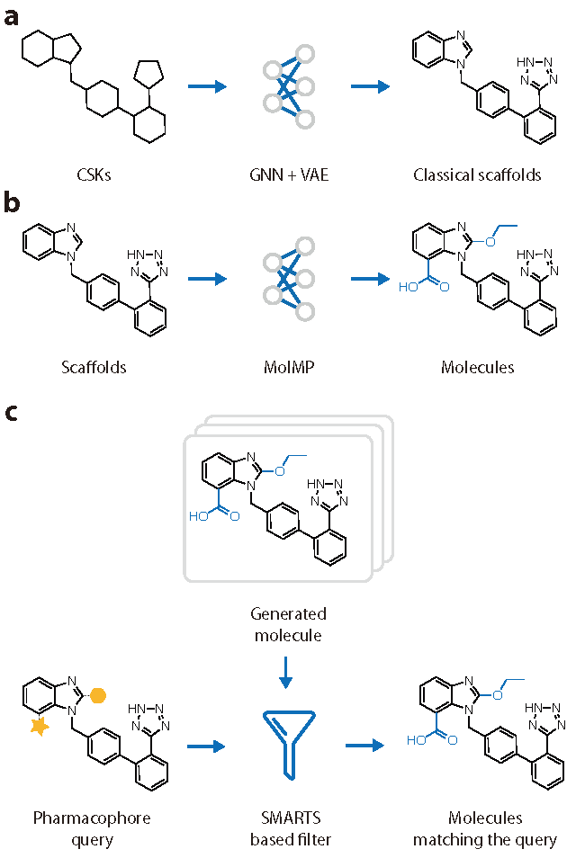
For convenience, we refer to the first type of structures as the “skeletons”, and the second type of structure as the “classical scaffolds”. To achieve those functionalities, DeepScaffold is composed of the following three components:

• A neural network for completing atom and bond type for cyclic skeletons (Figure 2a)

• A scaffold-based molecule generator (Figure 2b)

• A filter for side-chain properties based on pharmacophore queries (Figure 2c)

The three components are discussed in detail in the rest part of this section. We first discuss the dataset and data processing workflow in Section 2.2.The transformer from skeletons to scaffolds is discussed in Section 2.3, and the scaffold-based generator is discussed in Section 2.4. We briefly discuss the pharmacophore quires in 2.5 Finally, the evaluation methods are discussed in Section 2.6.

2.2 Dataset

Figure 3: a-d. The distribution of several important molecular properties (a for MW, b for LogP, c for QED, d for SAscore) of the extracted molecules. e. Workflow for scaffold extraction. Given the input molecule, the Bemis-Murcko scaffold is first extracted by removing all side chains. Other scaffolds are then obtained by recursively removing ring systems.

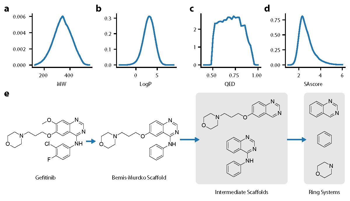
For model training, we use molecules from ChEMBL ²⁷, which is a widely used database containing both structural and bioactivity information for molecules. The data processing workflow largely follows that used in our previous study ¹⁸. First of all, the structural information of molecules represented as canonical SMILES are first extracted from ChEMBL dataset. The molecules are then standardized using RDKit, which involves the removal of salt and isotopes, as well as charge neutralization. Molecules containing elements outside the set {H, C, N, O, F, P, S, Cl, Br, I} are filtered from the dataset. Also, to make the dataset more suitable for drug design purposes, we only keep molecules with QED ²⁸ larger than 0.5. The final dataset (denoted as $\mathcal{M}=\{m_{i}\}_{i=1}^{N_{m}}$) contains $N_{m}=914464$ molecules. The distribution of several important molecular properties (including MW, LogP, QED and SAscore ²⁹) are visualized in Figure 3.

After the dataset is obtained, we need to extract scaffolds from each molecule. Previous researchers have developed many different ways to extract and organize scaffolds from structural data. Examples include HierS ⁷, SCONP ⁸, scaffold tree (ST) ⁹ and scaffold network (SN) ⁴. Here, we adopt the same scaffold extraction method as HierS. Compared with ST and SN, which are more widely adopted, HierS results in a fewer amount scaffolds, but is much easier to implement.

Molecules are composed of three components: ring systems (ring), side-chain bonds and atoms (chain), and linking bonds and atoms (linker). Atoms that are external to a ring but are bonded to a ring atom with a bond order greater than 1 are to be part of the ring system because they modify the nature of the ring. Atoms that are double-bonded to linker atoms are also considered to be part of the linker because they can modify the nature of the linker. The basis scaffolds for a molecule are the set of all unique ring systems in the molecule, where a ring system is defined as one or more rings that share an internal bond.

A recursive algorithm is used to elucidate all candidate scaffold structures including those derived from exhaustive combinations of the basis scaffolds. It recursively removes each ring system from the scaffolds of each level to generate fragments that contain all possible ring system combinations. Finally, the process is completed by adding the Bemis-Murko scaffold of the compound to the list of scaffold structures.

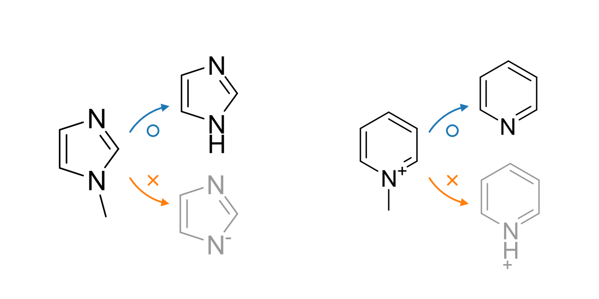
While removing chains/linkers connected on nitrogen atoms in aromatic rings, things become a little complicated. We have two choices to keep a molecule in correct valence while fracturing such bonds (Figure 4). It’s not in line with common sense about molecular scaffolds if a supplied scaffold has charges on some atom in it. Therefore we select the process above in Figure 4 to get the scaffold without any bonds connected with nitrogen atoms in aromatic rings, which can be an initiation point in the scaffold-based generative model. The indices of processed nitrogen atoms in each molecule are recorded in the scaffold extraction workflow as well, so as to modify it while generating a molecule.

Figure 4: Formal charges are removed and explicit hydrogen atoms are fixed after removing chains connected with nitrogen atoms in aromatic rings.

After all the distinct basis and multi-ring system scaffolds for each molecule have been identified and added to the scaffold list, hierarchical structural relationships between the scaffolds ($s\in\mathcal{S}$) and original compound ($m\in\mathcal{M}$) structures are established. Once all scaffolds are identified and their hierarchical relationships are established, the process can rapidly traverse the network of structural connections to determine relationships between indices of scaffolds and its original compounds.

Finally, to facilitate the sampling of training data during model optimization, we created indexes between skeletons ($c\in\mathcal{C}$), scaffolds ($s\in\mathcal{S}$) and molecules ($m\in\mathcal{M}$). Specifically, indices are created:

• From a given scaffold $s$ to its corresponding skeleton $c(s)$.

• From a given scaffold $s$ to the set of all molecules containing that scaffold $\mathcal{M}(s)$

• From a given molecule $m$ to the set of its sub-scaffolds $\mathcal{S}(m)$

2.3 Generating scaffolds from cyclic skeletons

As discussed in Section 2.1, to generate molecules from a given cyclic skeleton (CSK), we need to first generate a scaffold with atom types and bond types. To achieve this goal, we need to model a conditional distribution $p_{\boldsymbol{\theta}}(G_{s}|G_{c})$, where $G_{c}$ is the molecular graph of CSK $c$, and $G_{s}$ is the graph of the classical scaffold $s$.

2.3.1 The generative model

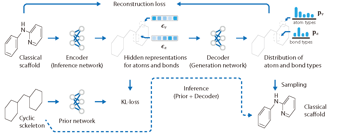
We construct the generation process as follows (see Figure 5):

Figure 5: The architecture of the model to transform CSKs to classicial scaffolds. Under the context of autoencoder, the entire model contains three components: the encoder, the decoder, and the prior network. During training, the reconstruction loss $\mathcal{L}_{\textrm{recon}}$ and the KL loss $\mathcal{L}_{\textrm{KL}}$ are calculated using the encoder, decoder and prior for model optimization. During inference, the latent variable is first sampled from the prior network and then fed into the decoder (or the generator network) to produce the classical scaffold.

• We first attach to each node $v$ and edge $e$ in $c$ a latent variable sampled from a prior distribution ${\boldsymbol{\epsilon}}_{v},{\boldsymbol{\epsilon}}_{e}\sim p_{\boldsymbol{\theta}}({\boldsymbol{\epsilon}}|G_{c})$. Here, we use a gaussian distribution with diagonal covariance structure to parameterize the prior: $p_{\boldsymbol{\theta}}({\boldsymbol{\epsilon}}|G_{c})=\mathcal{N}({\boldsymbol{\epsilon}};{\boldsymbol{\mu}}_{\boldsymbol{\theta}}^{\textrm{prior}}(G_{c}),{\boldsymbol{\sigma}}_{\boldsymbol{\theta}}^{\textrm{prior}}(G_{c})^{2}\mathbf{I})$

• The latent variables ${\boldsymbol{\epsilon}}_{v},{\boldsymbol{\epsilon}}_{e}$, together with the topological structure of the CSK, is fed into a graph convolutional neural network to generate a probability distribution of atom types for each node $\mathbf{p}_{v}$ and bond types for each edge $\mathbf{p}_{e}$.

• The types of each atom and bond in the output scaffold $s$ are then sampled from the distributions $\mathbf{p}_{v}$ and $\mathbf{p}_{e}$.

The latent variables are necessary to capture the probabilistic dependencies between different atoms and bonds. For convenience, we let ${\boldsymbol{\epsilon}}_{V}=[{\boldsymbol{\epsilon}}_{v}]_{v\in V}$ , ${\boldsymbol{\epsilon}}_{E}=[{\boldsymbol{\epsilon}}_{e}]_{e\in E}$, and ${\boldsymbol{\epsilon}}=[{\boldsymbol{\epsilon}}_{V},{\boldsymbol{\epsilon}}_{E}]$. Under the construction above, we can write the conditional distribution $p_{\boldsymbol{\theta}}(G_{s}|G_{c})$ as:

$$p_{\boldsymbol{\theta}}(G_{s}|G_{c})=\int_{{\boldsymbol{\epsilon}}}{p_{\boldsymbol{\theta}}(G_{s}|G_{c},{\boldsymbol{\epsilon}})p_{\boldsymbol{\theta}}({\boldsymbol{\epsilon}}|G_{c})}$$ (1)

2.3.2 Variational auto-encoder

A straight forward way of training such models is to maximize its likelihood value. However, as the model contains latent variables, calculating its likelihood value is not directly feasible. Therefore, we use variational inference to obtain a lower-bound of the likelihood. Specifically, we reformulate the model as a variational autoencoder ³⁰ by adding an auxiliary inference network $q_{\boldsymbol{\theta}}({\boldsymbol{\epsilon}}|G_{s},G_{c})$ to the model. Since $G_{s}$ already contains the full information of $G_{c}$, we shall write the inference network as $q_{\boldsymbol{\theta}}({\boldsymbol{\epsilon}}|G_{s})$. Similar to the prior, we use a diagonal Gaussian distribution for $q_{\boldsymbol{\theta}}$: $q_{\boldsymbol{\theta}}({\boldsymbol{\epsilon}}|G_{s})=\mathcal{N}({\boldsymbol{\epsilon}};{\boldsymbol{\mu}}_{\boldsymbol{\theta}}^{\textrm{post}}(G_{s}),{\boldsymbol{\sigma}}_{\boldsymbol{\theta}}^{\textrm{post}}(G_{s})^{2}\mathbf{I})$. In the context of autoencoders, the generator $p_{\boldsymbol{\theta}}$ is often referred to as "decoder", and the inference network $q_{\boldsymbol{\theta}}$ the "encoder". We then obtain the loss function as follows:

$$\mathcal{L}({\boldsymbol{\theta}})=-\mathbb{E}_{{\boldsymbol{\epsilon}}\sim q_{\boldsymbol{\theta}}}[\log{p_{\boldsymbol{\theta}}(G_{s}|G_{c},{\boldsymbol{\epsilon}})}]+KL(p({\boldsymbol{\epsilon}})||q_{\boldsymbol{\theta}}({\boldsymbol{\epsilon}}|G_{s},G_{c}))$$ (2)

The first term and second term in eq.2 are usually called the reconstruction loss ($\mathcal{L}_{\textrm{recon}}$) and the KL loss ($\mathcal{L}_{\textrm{KL}}$) respectively. Minimizing the loss eq.2 is maximizing a lower bound on the likelihood function eq.1.

2.3.3 Graph convolutional neural network

The encoder $q_{\boldsymbol{\theta}}({\boldsymbol{\epsilon}}|G_{s})$, decoder $p_{\boldsymbol{\theta}}(G_{s}|G_{c},{\boldsymbol{\epsilon}})$, as well as the prior network $p_{\boldsymbol{\theta}}({\boldsymbol{\epsilon}}|G_{c})$ are all parameterized using graph convolutional neural networks (GNN). The architecture is shown in Figure 6.

Figure 6: The architecture of the graph convolutional neural network (GNN). Before feeding into the GNN, two transformations are performed on the original molecular graph $G$: a. Virtual bonds are added to capture remote connectivity relationship. b. The atoms and bonds are treated equally as "nodes" in the new graph. c. Adding a hierarchical organization to the molecular graph

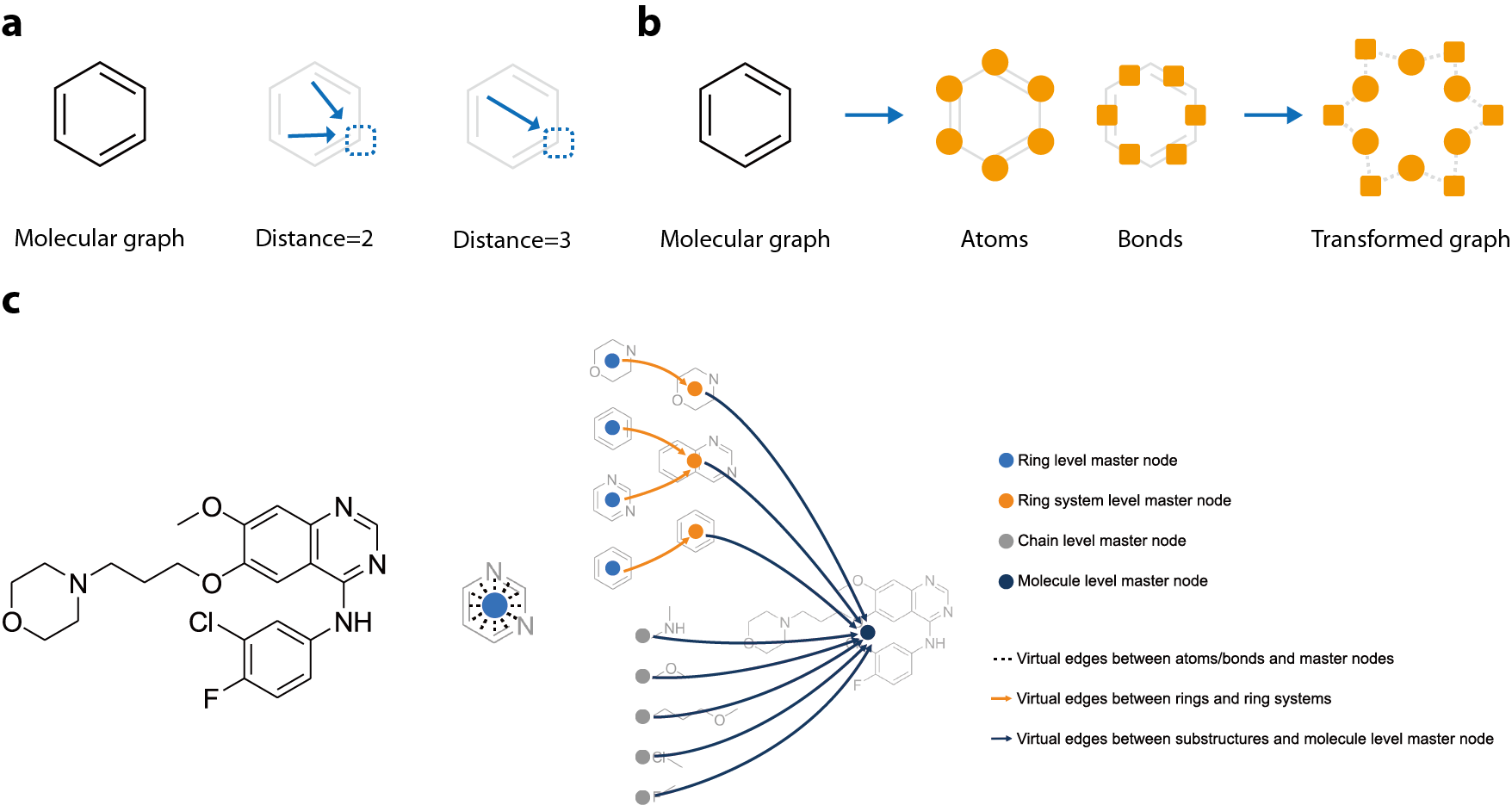
Before entering the graph convolutional network, we perform the following transformations to the input graph $G=(V,E)$:

• Virtual bonds are added to capture remote connectivity relationship. Specifically, we add new bonds between atom pairs separated by two or three bonds, similar to our previous works ¹⁸. We also create new bond types for those virtual connections to separated them from real chemical bonds. The molecular graph with virual bonds are denoted as $G^{(1)}=(V^{(1)},E^{(1)})$.

• $G^{(1)}$ is then transformed into a new graph $G^{(2)}=(V^{(2)},E^{(2)})$ by treating atoms and bonds in $G^{(1)}$ equally as nodes in $G^{(2)}$. In other words, we have $V^{(2)}=V^{(1)}\cup E^{(1)}$, and $E^{(2)}=\{\{v,e\}|v\in V^{(1)},e\in E^{(1)}\textrm{ and }v\in e\}$.

• For each ring $R$ in the graph $G$, we add a virtual node $v_{R}$ to the $G^{(2)}$, and connect it to each element inside the ring $R$ in graph $G^{(2)}$. Similar operations are performed for each linker in $G$. In terms of ring assemblies, virtual nodes are added and are connected to virtual elements representing rings. The overall effect is shown in Figure 6c.. The transformed graph is denoted as $G^{(3)}=(V^{(3)},E^{(3)})$

After those transformations, the graph $G^{(3)}$ is then sent to the graph convolutional network as input. Each convolution operation is composed of three stages:

• Broadcasting: The information of nodes are broadcasted to edges. Specifically, for each edge $e=\{u,v\}\in E^{(3)}$, the representation of terminal nodes $\mathbf{h}_{u}$ and $\mathbf{h}_{v}$ are broadcasted to edge $e$ as

  $$\mathbf{h}_{e}=\textrm{MLP}^{\textrm{broadcast}}([\mathbf{h}_{u},\mathbf{h}_{v}])$$ (3)

  $[\cdot,\cdot]$ is the concatenation operation for vectors. $\textrm{MLP}^{\textrm{broadcast}}$ is a linear layer with BN-ReLU-Linear architecture.

• Gathering: The information broadcasted to each edge is again gathered to each node. We use to ways to gather information from edges: summation and maximization. The edge representation is firstly split into two parts:

  $$[\mathbf{h}_{e}^{\textrm{max}},\mathbf{h}_{e}^{\textrm{sum}}]=\mathbf{h}_{e}$$ (4)

  vectors $\mathbf{h}_{e}^{\textrm{max}}$ are subjected to maximization:

  $$\mathbf{h}_{v}^{\textrm{max}}=\max_{e\in E^{(3)}\textrm{and}v\in e}{\mathbf{h}_{e}^{\textrm{max}}}$$ (5)

  vectors $\mathbf{h}_{e}^{\textrm{sum}}$ are subjected to summation:

  $$\mathbf{h}_{v}^{\textrm{sum}}=\sum_{e\in E^{(3)}\textrm{and}v\in e}{\mathbf{h}_{e}^{\textrm{sum}}}$$ (6)

  The results are concatenated:

  $$\mathbf{h}_{v}^{\textrm{gather}}=[\mathbf{h}_{v}^{\textrm{max}},\mathbf{h}_{v}^{\textrm{sum}}]$$ (7)

• Updating: The representation of each node is updated using the gathered information:

  $$\mathbf{h}_{v}^{\textrm{new}}=\textrm{MLP}^{\textrm{update}}([\mathbf{h}_{v},\mathbf{h}_{v}^{\textrm{gather}}])$$ (8)

  $\textrm{MLP}^{\textrm{update}}$ is a linear layer similar to $\textrm{MLP}^{\textrm{broadcast}}$

2.3.4 Training details

The model is validated using the holdout method. 80% of scaffolds are used for training (denoted as $S^{\textrm{train}}$), and the remaining 20% is used for testing (denoted as $S^{\textrm{test}}$). The metrics used for test set evaluation is discussed in detail in Section 2.6.1. The mini-batches $B=\{s_{i},c_{i}\}_{i=1}^{|B|}$ used at each step for model training is constructed by first sampling the scaffolds ($\{s_{i}\}_{i=1}^{|B|}$) are then finding their corresponding cyclic skeleton $c_{i}=C(s_{i})$. Naive VAE tends to suffer from the problem of posterior collapse. To encourage the model to encode more information into the latent variable, we experimented several attempts, including KL-annealing (proposed in ³¹) and $\beta$-VAE (proposed in ³²).

AdaBound is used for model optimization, with the initial learning rate set as $1\times 10^{-3}$, and the final learning rate as $0.1$. This means that the optimizer will gradually anneal from an Adam optimizer with learning rate $1\times 10^{-3}$ to an SGD optimizer with learning rate $0.1$. The gradient is clipped to [-3, 3] to improve model stability. The dimension of latent variables ${\boldsymbol{\epsilon}}_{v},{\boldsymbol{\epsilon}}_{e}$ is set to be 10. We performed experiments with more latent variables, but found little improvement in model performance.

2.4 Scaffold-based molecule generation

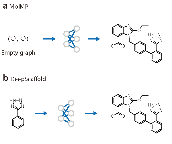
Now we introduce the model used for scaffold derivatization. The central goal of this task is to reconstruct the side-chains based on the structural information of the scaffold. Formally speaking, we are modeling the conditional distribution $p_{\boldsymbol{\theta}}(x|s)$, where $s$ is the scaffold and $x$ is the full molecule. The generation process of side-chain follows largely from our previous work ¹⁸. The major difference is that for scaffold-based generation, the process starts from the graph of the given scaffold, instead of an empty graph (see Figure 7). The model builds the molecule in a step-by-step fashion. At each step, the model needs to decide which of the following actions to perform: (1) append a new atom to the graph, (2) connecting two existing nodes or (3) to terminate the generation process. The architecture of graph convolutional layer is similar to that used in ¹⁸. In terms of the model architecture, a 20 layer densenet is used in this model, similar to Section 2.3. The growth rate is set to 24, and the number of features in each bottleneck layer is set to 96. We use the likelihood-based loss function for model optimization. Importance sampling is used to improve the performance of the model (following ¹⁸). The value for the hyperparameter $k$ (the number of samples generated from importance sampling) and $\alpha$ (parameter controlling the degree of uncertainty in route sampling) is set as $5$ and $0.5$ respectively.

Note that our proposed model share similarity with that by Lim et. al. Both methods share the idea of growing the molecule directly from the scaffold. However, we improve upon the work by Lim et. al. from the following perspectives:

• Beside including Bemis-Murko scaffolds of molecules, we also included all its sub-scaffolds within our dataset (under the definition of HierS, see Section 2.2 for details). This treatment will have two advantages for the model.

  • First of all, expanding the scaffold set $\mathcal{S}$ will reduce the chance of missing potential bioactive scaffolds, making the dataset more fitted to the practical need.

  • Secondly, the definition of Bemis-Murko scaffold has excluded all ring-based structures from the side-chain, making it overly restricted for situations in medicinal chemistry. By including the sub-scaffolds, we can significantly increase the structural diversity of the substituents in the scaffold, thereby expanding the practicality of our model.

• Compared with Lim et. al., we include a much wider range of metrics for model evaluation (see 2.6), including MMD, internal diversity, docking score and so on. We also include case studies related to scaffold-based drug discovery for GPCRs.

Model validation is performed in the following two ways:

2.4.1 Holdout validation

Holdout method is mainly used to obtain an overall view of the model’s performance. The set of all molecules is split into two portions: the training set (80%) and the test set (20%), used respectively for model optimization and evaluation. Note that is method will result in an overlap of scaffold set between the training and test set, therefore can not be used to examine the model’s ability to generalize to new scaffolds.

2.4.2 Leave-one-out validation

Leave-one-out validation is carried out in the following way: Given a scaffold of interest, we gather all molecules containing this scaffold as substructure, and exclude those molecules from the training set. Following this method, there will be no overlap of scaffolds and molecules between training and test set. However, it is impractical to perform such validation to all 338,932 extracted scaffolds. Therefore, we selected three scaffolds as a case study, as shown in Figure 13. All scaffolds selected are privileged scaffolds for G-protein-coupled receptors (GPCRs) .

Model optimization is performed using Adam optimizer. The learning rate is set to 0.001 in the first step, and decay at a rate of 0.99 for every 100 steps, until the minimum learning rate $5\times 10^{-5}$ is reached. Regularization techniques such as dropout or weight decay are not used in this model. To stabilize training, the gradient is clipped to [-3.0, 3.0] at each optimization step. Training is performed for 50,000 iterations, taking roughly 20 hours to complete.

Figure 7: The generation process. a. Unconditional generative models (such as MolMP) starts molecule generation from empty graph $G_{0}=(,)$. b. DeepScaffold starts molecule generation directly from scaffolds.

At each step, we need to sample a mini-batch of scaffold-molecule pairs ($B=\{s_{i},m_{i}\}_{i=1}^{|B|}$) from the training set. The batch size $|B|$ is set to 128. Note that there are many different ways to perform the sampling from the training set. For example, we can first sample a set of scaffolds $\{s_{i}\}_{i=1}^{|B|}$ and then assign each scaffold $s_{i}$ with a molecule drawn from $M(s_{i})$. We can also sample molecule first and scaffold next. The impact of different sampling algorithm is analyzed in Supporting Information. The result can be summarized as follows: (1) If we place equal weight to each scaffold, the molecules will be sampled disproportionately. (2) If we place equal weight to each molecule, the scaffolds will then be sampled disproportionately. In a word, it is quite difficult to balance both scaffold and molecule. As a result, we construct each mini-batch using a mixture of samples from both sampling methods. Here, we use equal weights for each sampling method. In future works, the weight can be treated as a hyperparameter and be subjected to optimization and tuning.

2.5 Using scaffold and pharmacophore as queries for generation

For medicinal chemists, it is would often be useful to have the ability to specify the property of substituents at specific locations during scaffold-based molecule design. This may happen when we have clear SAR information concerning the given scaffold. In this work, we also created a tool to use both scaffold and pharmacophore queries during molecule generation. The implementation of this functionality is rather simple: after the molecules are generated from the scaffold using the method discussed in Section 2.4, we filter those results against the user’s queries. We currently allow users to specify the size of the side-chain (measured using the number of heavy atoms ), whether to have hydrogen bond donors (HBD) and whether to have hydrogen bond acceptors (HBA). We plan to increase the spectrum of supported queries in the future.

2.6 Evaluation

2.6.1 Generating scaffolds from cyclic skeletons

We use the following metrics for model evaluation:

Reconstruction loss, KL loss and total loss VAE learn the generative model by trying the achieve the best reconstruction using the least information. The reconstruction loss $\mathcal{L}_{\textrm{recon}}$ measures the accuracy of reconstruction for the autoencoder, while the KL loss $\mathcal{L}_{\textrm{KL}}$ measures the amount of information stored inside the latent variable. The total loss $\mathcal{L}_{\textrm{total}}$, which is also used during the model training, is the sum of reconstruction loss and KL loss.

Chemical validity Given a cyclic skeleton $c$, we measure the chemical validity of output scaffolds generated from skeleton $c$. The validity of a given molecule is evaluated using the Chem.Sanitize API provided by RDKit. The validity is measured by the percent valid output calculated as follows:

$$P_{c}^{\textrm{valid}}=N_{c}^{\textrm{valid}}/N_{c}^{\textrm{total}}$$ (9)

where $N_{c}^{\textrm{valid}}$ is the number of valid outputs and $N_{c}^{\textrm{total}}$ is the number of total outputs. Those values are averaged among all cyclic skeletons, and the final value $\bar{P}_{\textrm{valid}}$ is reported.

2.6.2 Evaluating scaffold-diversification model

In order to evaluate the performance of the scaffold-based molecular diversification model, we gather all scaffolds occurred inside the test set, and remove those with less than 10 corresponding molecules. After obtaining the set of scaffolds to be evaluated (denoted as $S_{\textrm{test}}$), 10,000 sample molecules are generated for each scaffold, and the evaluation of those samples is carried out using the following metrics.

Chemical validity and uniqueness We first measure the chemical validity and uniqueness of the generated molecules. The validity of a given molecule is evaluated using the Chem.Sanitize API provided by RDKit. For a given scaffold $s$, we obtaining the number of valid outputs (denoted as $N_{s}^{\textrm{valid}}$), and divide it with the total number of generated molecules (denoted as $N_{s}^{\textrm{total}}$). The percentage of valid outputs are calculated using eq.10.

To calculate the uniqueness, we remove all duplicated molecules from the valid outputs, and calculate the number of remaining molecules (denoted as $N_{s}^{\textrm{uniq}}$). The uniqueness is calculated using eq.11.

$$P_{s}^{\textrm{valid}}=N_{s}^{\textrm{valid}}/N_{s}^{\textrm{total}}$$ (10)

$$P_{s}^{\textrm{uniq}}=N_{s}^{\textrm{uniq}}/N_{s}^{\textrm{valid}}$$ (11)

$P_{s}^{\textrm{valid}}$ and $P_{s}^{\textrm{uniq}}$ scores are calculated for each scaffold inside the test dataset, and the average values of the two metrics ($\bar{P}_{\textrm{valid}}$ and $\bar{P}_{\textrm{uniq}}$) are reported. The distribution of the two metrics among all test set scaffolds is also reported. Also, we will discuss how scaffold sizes would affect those two performance metrics.

Distribution of molecular properties Next, we investigate the model’s ability to correctly model the distribution of several important molecular properties. Here we consider the following three properties: molecular weight (denoted as $MW$), log partition coefficient (denoted as $\textrm{log}P$) and the drug-likeness score (measured by QED ²⁸). All properties above can be calculated using RDKit.

For each scaffold $s$ in the test set, we compare the mean and standard deviation of each property ($MW$, $\textrm{log}P$ and $QED$) between the molecules generated and molecules in the test set. Previous studies have used metrics such as $D_{KL}$ and $D_{JD}$ to quantify the difference. The approach adopted here is simpler, but offers higher interpretability compared with $D_{KL}$ and $D_{JD}$. For a quantitative evaluation, we instead use maximum mean discrepancy (MMD), as discussed in Section 2.6.2.

Diversity Output diversity is another important metric for evaluating molecular generative models. Although, as discussed in Section 2.6.2, the standard deviation of molecular properties could, in some extent, reflect the structural diversity of the generated outputs, a more rigorous definition of structural diversity is needed for quantitative evaluation. Here, we adopt the formulation of internal diversity proposed by Benhenda et. al³³. Supposed the molecules are sampled from a molecule distribution $x\sim p(x)$, the structural diversity of this distribution can be defined as:

$$I=1-\mathop{\mathbb{E}}_{x,y\sim p}[k(x,y)]$$ (12)

Where $k(x,y)$ is the similarity of the two molecules $x$ and $y$. Here, we use the tanimoto score of the Morgan fingerprints between the two molecules as the similarity measurement. Intuitively speaking, the structural diversity of $p$ is defined as one minus the average similarity between two randomly sampled molecules from $p$. We can estimate the value of $I$ from samples $\{x_{i}\}_{i=1}^{N}$ drawn from $p$:

$$\hat{I}_{U}=1-\frac{\sum_{i=1}^{N}\sum_{j=1,j\neq i}^{N}k(x_{i},x_{j})}{N(N-1)}$$ (13)

It can be proved that $\hat{I}_{U}$ is an unbiased estimator of $I$. Note that this estimator is slightly different from that originally proposed by Benhenda et. al. ³³:

$$\hat{I}_{V}=1-\frac{\sum_{i,j=1}^{N}k(x_{i},x_{j})}{N^{2}}$$ (14)

It can be shown that $\hat{I}_{V}$ is equals to $\frac{N-1}{N}\hat{I}_{U}$, and therefor a biased V-staticstics for $I$. Also, it can be shown that the bias of $\hat{I}_{V}$ depends on the sample size $N$, and will be larger in smaller datasets. This could be problematic for two ways: First, many scaffolds in the test set have only a small number of corresponding molecules, which may increase the bias. Second, the sample size ($N$) of the test set is usually smaller than that of the generated samples, which will bring additional bias to the result. Therefore, the U-statistics $\hat{I}_{U}$ is instead used in this paper for the calculation of internal diversity.

Maximum mean discrepancy (MMD) The central task of scaffold-based diversification is to model the conditional distribution $p(x|s)$ of molecular structure $x$ given the scaffold $s$. Therefore, the most natural way of evaluating such models would be measuring the dissimilarity between the ground truth distribution $p_{d}(x|s)$ and the modeled distribution $p_{g}(x|s)$. Maximum mean discrepancy (MMD) is one of such metrics that have been widely applied in generative modeling (both for model training ³⁴ and evaluation ³⁵). Different from other metrics, such as Jensen–Shannon divergence (JSD), Wasserstein distance (WD) ³⁶ or Frechet ChemNet distance (FCD) ³⁷, MMD does not require additional discriminator or preditor to be evaluated, which makes it much easier to calculate.

Given the samples from two probability distribution $\{x_{i}\}_{i=1}^{N}\sim p_{d}$, $\{y_{i}\}_{i=1}^{M}\sim p_{g}$, the MMD between the two distribution can be estimated as:

$$\hat{D}=\frac{1}{N(N-1)}\sum_{i=1}^{N}\sum_{j=1,j\neq i}^{N}k(x_{i},x_{j})+\frac{1}{M(M-1)}\sum_{i=1}^{M}\sum_{j=1,j\neq i}^{M}k(y_{i},y_{j})-\frac{2}{MN}\sum_{i=1}^{N}\sum_{j=1}^{M}k(x_{i},y_{j})$$ (15)

Where $k(\cdot,\cdot)$ is the kernel function. Similar to Section 2.6.2, we choose the tanimoto similarity between molecules as $k$. It can be proved that tanimoto similarity is in fact a legitimate kernel function ³⁸.

One of the most important applications the model is the design of molecule-based on privileged scaffolds. Ideally, given a known bioactive scaffold, the generated molecule should also be bioactive. To test whether the model possess such desirable property, we examine:

• The ability for the generative model to reproduce known active molecules

• The (predicted) bioactivity of the output molecules for the target.

The rate of reproduced active compounds First of all, the rate reproduced active molecules (denoted as $R$) for GPCRs is reported. Specifically, we collect all molecules that are active against at least one target in the GPCR family (denoted as the set $T_{\textrm{GPCR}}$), and examine how many of them appear in the set of molecules sampled from the model(denoted as $M_{s}$):

$$R_{\textrm{GPCR}}=\frac{|M_{s}\cap T_{\textrm{GPCR}}|}{|T_{\textrm{GPCR}}|}$$ (16)

We also investigate the ability for the model to reproduce known drugs, by collecting all drugs (denoted as $T_{\textrm{drug}}$) from the test set, and calculate the ratio $R_{\textrm{drug}}$:

$$R_{\textrm{drug}}=\frac{|M_{s}\cap T_{\textrm{drug}}|}{|T_{\textrm{drug}}|}$$ (17)

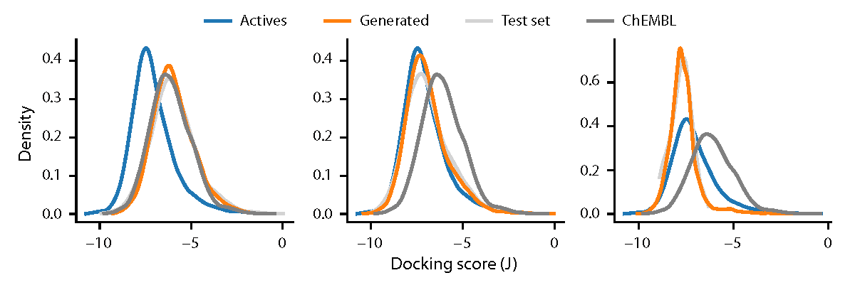
Docking Next, we report the predicted activity of output molecule for GPCRs. It is impractical to evaluate the output molecule against all targets in the GPCR family. Instead, we choose Dopamine Receptor D2 (DRD2) as a representative, which is a well-studied target for antipsychotic drugs ³⁹. The predicted activity for DRD2 is calculated using docking. The bioactivity model for DRD2 is built following Supporting Information:

For each bioactive scaffold selected for GPCRs, a comparison of docking scores was carried out between four sets of compounds: (1) samples generated by the model, (2) molecules inside the test set, (3) known actives for DRD2 and (4) randomly sampled molecules from ChEMBL. A well-performing generative model should result in a similar distribution of docking scores between (1) and (2). Also, the average score for (1) should be close to (3), and better than (4).

Structural distribution of side-chains Given the set of generated molecules given a scaffold, users can further filter the result by adding requirement on the properties of side-chains attached to the scaffold. Since different users may require different types of substitution in different locations, the model needs to generate a diverse set of side-chain configurations in order to handle the user’s requirements efficiently. Therefore, for each scaffold in the leave-one-out evaluation (see Section 2.4.2), we analyze the location and size of each side-chain in the generated molecules in order to evaluate the diversity of side-chains. We also compare the result with test set molecules to determine the quality of the generated samples.

3 Results

3.1 Generated samples

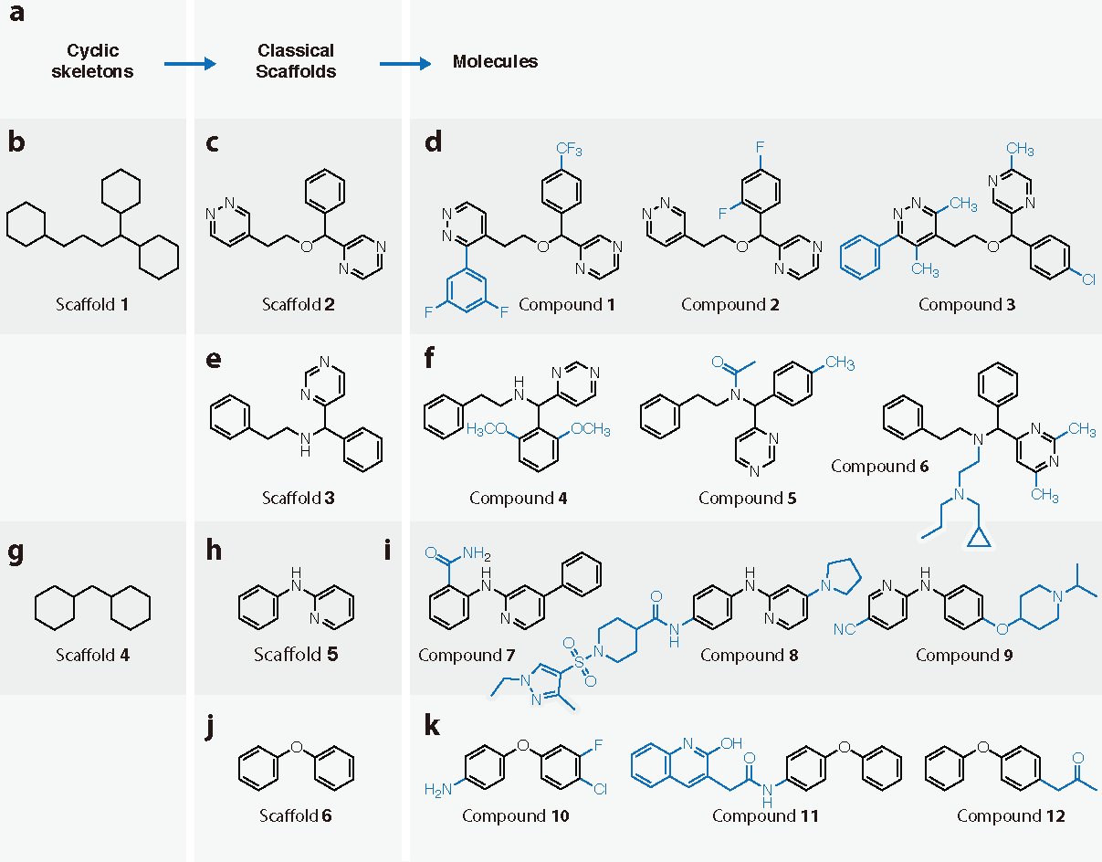
Before diving into model’s performance, we present a brief view of DeepScaffold by showcasing several generated molecules from cyclic skeletons as well as classical scaffolds using the model. The result is demonstrated in Figure 8. Two cyclic skeletons, scaffold 4 (Figure 8 g), with a relatively simple structure, as well as the more complexed scaffold 1 (Figure 8 b), are selected from the hold-out test set. For each scaffold, we generate two classical scaffolds (scaffold 2 (Figure 8 c) and scaffold 3 (Figure 8 e) for scaffold 1, as well as scaffold 5 (Figure 8 h) and scaffold 6 (Figure 8 j) for scaffold 4 and structural derivification is performed on those structures (Figure 8 d,f,i,k).

Figure 8: Generated samples from DeepScaffold.

3.2 Generating scaffolds from cyclic skeletons

The performance of the proposed model is evaluated following Section 2.6.1, with results shown in Table LABEL:tab:csk.

First of all, it is shown that approaches such as KL-annealing and $\beta$-VAE all showed positive results in solving posterior collapse. Both VAE + annealing and $\beta$-VAE are capable of achieving higher $\mathcal{L}_{\textrm{KL}}$. Notably, by using annealing, the model can achieve a slightly better $\mathcal{L}_{\textrm{total}}$ with a much higher $\mathcal{L}_{\textrm{KL}}$. In terms of the output validity, $\beta$-VAE (with $\beta$ value set to 0.5) can achieve the best performance of 82.5%. Interestingly, the output validity is not always consistent with the performance measured using $\mathcal{L}_{\textrm{total}}$. In the future, we plan to utilize more recent techniques in VAE training in order to improve the result, such as using more complexed prior ⁴⁰ posterior ⁴¹.

Table 1: Generating scaffolds from cyclic skeletons

Model	%valid	%recon	$\mathcal{L}_{\textrm{KL}}$	$\mathcal{L}_{\textrm{recon}}$	$\mathcal{L}_{\textrm{total}}$
$\beta$-VAE ($\beta=0.5$)	82.50%	61.00%	9.82	1.11	10.93
$\beta$-VAE ($\beta=0.$1)	80.70%	91.30%	14.15	0.23	14.38
VAE + KL annealing	76.80%	10.00%	5.02	4.38	9.4
VAE	68.50%	6.32%	3.37	6.06	9.43

3.3 Scaffold derivation

3.3.1 Validity and uniqueness

Figure 9: Sample validity and uniqueness. a. The average validity (98.8%) and uniqueness (69.1%) among all scaffolds. b. The relationship between the molecular weight of each scaffold and the (logit) precent-valid output. c. The relationship between molecular weight for each scaffold and (logit) percent unique output. d-e. Several generated samples using scaffolds with d. high molecular weight and e. low molecular weight.

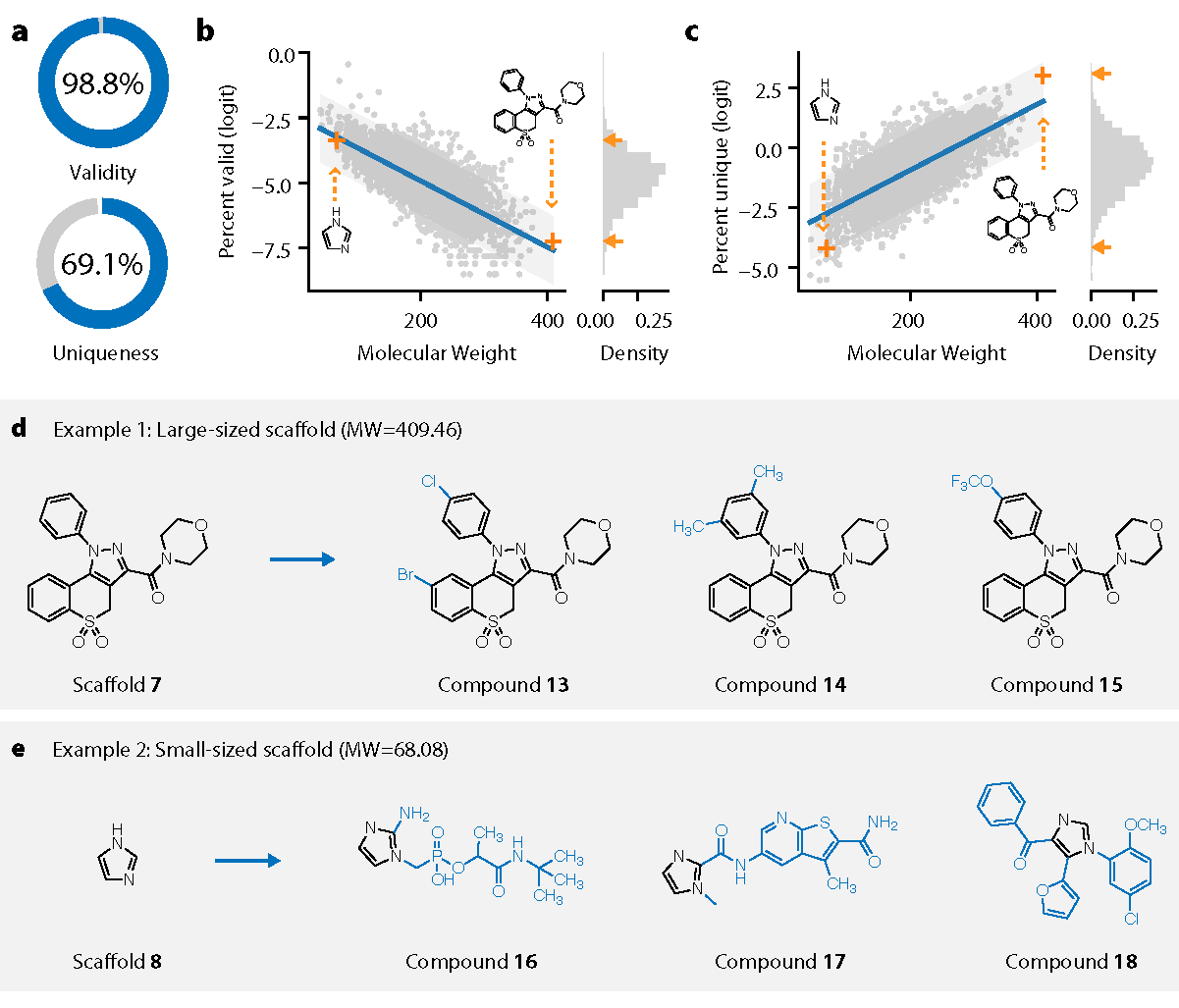
The performance of scaffold-based molecular diversification in terms of validity and uniqueness is summarized in Figure 9. Among all scaffolds, the average percentage of valid output ($\bar{P}_{\textrm{valid}}$) is 98.9%, and the average percentage of unique output is 69.1% ($\bar{P}_{\textrm{uniq}}$), as shown in Figure 9. It is immediately noticed that the result in $\bar{P}_{\textrm{valid}}$ and $\bar{P}_{\textrm{uniq}}$ is significantly different from the results produced by the unconditional version of the model with similar architecture ¹⁸. Specifically, the scaffold-based model can achieve a higher precent-valid value, while having a lower percent unique value. A similar result was reported by Lim et. al. ²⁶ using a different dataset including BM scaffolds.

To better understand the phenomenon, we further investigate the relationship between the scaffold size (measured by the molecular weight of the scaffold $MW_{s}$) and the performance of the two metrics. The result is shown in Figure 9 and Figure 9. It can be shown that $MW_{s}$ is positively correlated with $P_{s}^{\textrm{valid}}$ (correlation coefficient $r=$0.73, significance level $p<0.001$ ), while negatively correlates with $P_{s}^{\textrm{uniq}}$ (correlation coefficient $r=$-0.66, significance level $p<0.001$). This means that larger scaffolds tend to have higher output validity, but lower uniqueness. The result is in fact inline with the mode of thinking in medicinal chemistry: for smaller scaffold, there is usually a plenty of room for structural diversification, while for larger scaffolds, in order to achieve higher drug-likeness and synthetic accessibility, the size and diversity of structural modification are much more restricted, resulting in a higher chance of duplicates. Also, smaller side-chains means fewer generation steps, which will, therefore, reduce the chance of validity violation during generation. Two representative scaffolds are chosen from the test scaffold set and are shown in Figure 9 and Figure 9. Consistent with the analysis above, the side-chains attached to the smaller scaffold is larger and more diverse, and those attached to the larger scaffold have a much simpler structure.

The discussion above also provides some important insight into how future benchmarks should be constructed for this type of model. First of all, since the evaluation metrics such as $P_{s}^{\textrm{valid}}$ and $P_{s}^{\textrm{uniq}}$ depends on the scaffold $s$ chosen for evaluation, it is important to use a common scaffold set as the test set during model comparisons. Secondly, it will be better to perform the evaluation in a per-scaffold fashion. Specifically speaking, instead of comparing the average validity and uniqueness between models, it will be better to perform paired tests of those metrics.

3.3.2 Molecular properties

Figure 10: Comparing the distribution of several molecular properties (MW, LogP and QED) between generated and test set molecules. For each subplot, the horizontal coordinate indicates the statistics (a-c for mean and d-f for standard deviation) of a molecular property (a and d for MW, b and e for LogP, c and f for QED) of generated molecules, while its y coordinate indicates that statistics for the test set molecules. Scaffolds with more than 400 corresponding molecules (that is, $|\mathcal{M}(s)|>400$) are highlighted in blue.

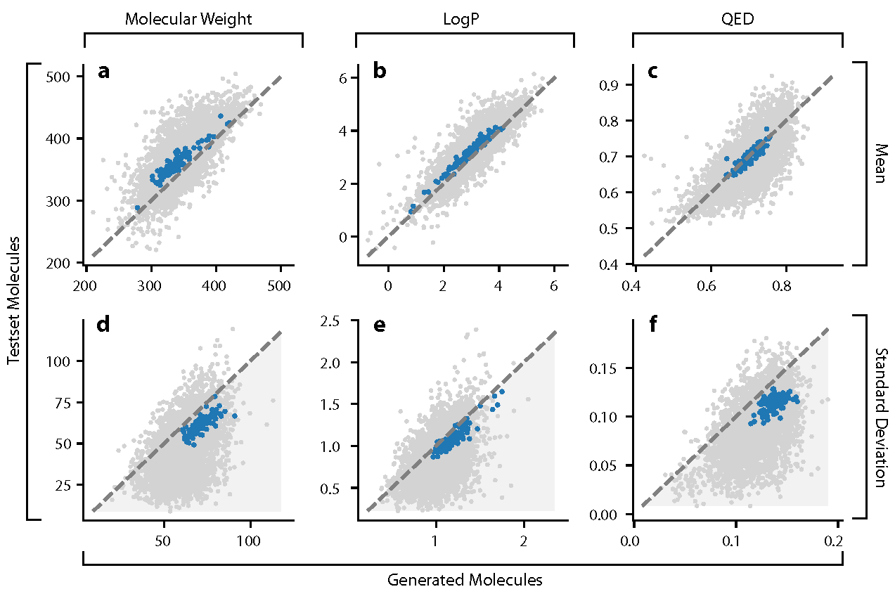
Next, the distributions of molecular properties for generated molecules are analyzed and compared with that in the test set. The results are summarized in Figure 10. Each point in the scatter point corresponds to a scaffold in the test set. Its horizontal coordinate indicates the statistics (mean or standard deviation) of a molecular property (MW, LogP or QED) of generated molecules, while its y coordinate indicates that statistics for the test set molecules. Scaffolds having more than 400 corresponding molecules in the test set are lighted in blue.

We first examine the mean statistics of molecular properties. Form Figure 10, it can be observed that, for all three properties, the points in the scatter plot lies relatively close to the diagonal line, demonstrating that the model is performing well in modeling the means of those properties. It is also noted that scaffolds with more molecules (highlighted in blue) lies much closer to the diagonal line compared with other scaffolds. This may indicate better performance in scaffolds with more data points.

However, in terms of standard deviation, there is a large discrepancy between the generated and test samples. It is observed that a large number of data points lies below the diagonal line, which indicates that the generated molecule usually have a more dispersed distribution of molecular properties. This is ,in fact, a result of higher structural diversity of output molecules, as is shown in Section 3.3.3. Again, highlighted points are observed to lie much closer to the diagnal line, showing that the model performs much better on those scaffolds compared with the rest.

3.3.3 Molecule diversity

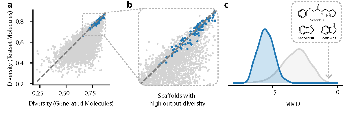
We subsequently analyze the internal diversity of the sampled and test set molecules, with results summarized in Figure 11. Similar to the result showed in Figure 11, we have observed that most data points lie below the diagonal line, indicating a higher structural diversity of sampled molecules compared with test set molecules. Also, a similar result is observed that scaffolds with more data in the training set perform much better compared with other scaffolds (see the data points highlighted in blue).

3.3.4 MMD

The result for MMD is shown in Figure 11. The grey curve shows the distribution of MMD among all test set scaffolds, while the blue curve shows the distribution of MMD among scaffolds with more than 400 related molecules. It can be immediately observed from the figure that the model performs significantly better for scaffolds included in the blue line.

Figure 11: Internal diversity and MMD. a. Comparing the internal diversity between generated molecules and testset molecules. Scaffolds with more than 400 corresponding molecules (that is, $|\mathcal{M}(s)|>400$) are highlighted in blue. b. Scaffolds with high output diversity. c. The distribution of MMD among all scaffolds in the test set. Scaffolds with more than 400 corresponding molecules are highlighted in blue.

3.3.5 Analyzing bad-cases

In summary, the evaluation results reported in the above sections lead to the following conclusions regarding the model’a performance:

• With a given scaffold, molecules generated by the model tend to be more structurally diverse compared with the molecules containing that scaffold in the test set

• The distribution of generated molecules matches better with that of the test set molecules for scaffolds that occurs more frequently.

In order to get a better understand those phenomenons, we performed a bad-case analysis considering scaffolds with lowest MMD values, as demonstrated in Figure 12. Generated molecules for those scaffolds are shown in Figure 12, while molecules containing those scaffolds in the test set are shown in Figure 12.

As we examine the results in Figure 12, we can immediately notice the low structural diversity for the test set molecules. Interestingly, after inspecting the origin of those molecules in the ChEMBL dataset, we found that those molecules are mostly collected from a single publication or a single assay: All molecules containing scaffold 9 is originated from the assay CHEMBL3707834, and all molecules containing scaffold 10 is originated from the assay CHEMBL3705917. 89% of molecules containing scaffold 11 is collected from the publication CHEMBL1144160. In other words, for each scaffold shown in Figure 12, its corresponding molecules are largely designed by the same group of researchers under a same target.

Figure 12: Demonstration of several bad-cases drawn from the test set scaffolds.

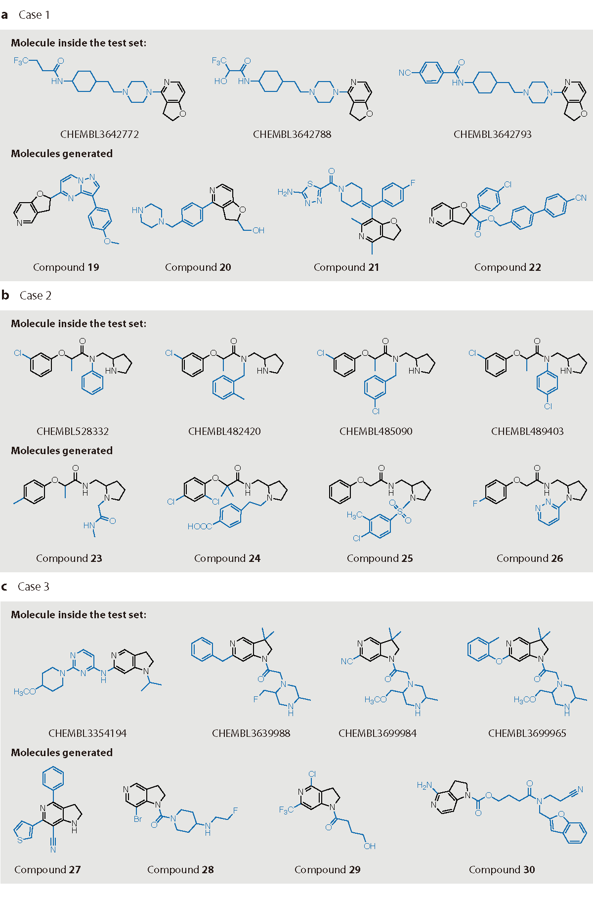
The observations above can offer an explanation to the seemly bad performance of the model. It can be concluded that the test set for scaffold 9-11 suffers from the non-random-sampling bias: the molecules is sampled from a much more restricted chemical space that reflects the preference of specific research or publication. Therefore, the performance of the model will be underestimated, resulting in high MMD values, as well as large discrepancy between structural and property distributions. On the contrary, a higher diversity among generated molecule is a sign that the model did not memorize the side-chain distribution for each scaffold, indicating high generalizability.

The foregoing discussion proposes a challenge for model evaluation in scaffold-diversification tasks. In order to obtain a good assessment for the model’s performance, it is necessary to use a test set that is unbiased in molecule distribution. Future research may explore the potential of developing an unbiased benchmark set for scaffold-diversification models. Another solution would be introducing sample weight during evaluation to mitigate the non-random-sampling bias, which will be left for future researches.

3.3.6 Case study: privileged scaffolds for GPCRs

As described in Section 2.4.2, three privileged scaffolds for GPCRs (shown in Figure 13) are selected for the case study. We performed leave-one-out evaluation for each scaffold, with the results summarized in Table LABEL:tab:scaffold and Figure 13.

The model performs well on the percentage of valid outputs, with values closing to 100%. The uniqueness for scaffold 12 and 13 is 86.6% and 87.7% respectively, while for 14, the value is of 45.4%. This smaller value might result from the higher structural complexity of scaffold 14, which may restrict the chemical space of the side chains. Similar to the results demonstrated in Section 3.3.2 and Section 3.3.3 generated molecules have a wider distribution of MW, LogP and QED, and is more structurally diverse compared to real samples. In terms of MMD, we found that scaffold 14 have a significantly lower MMD value compared with scaffold 12 and 13. The high MMD value can largely be contributed to the non-random-sampling bias in the test set. In fact, most scaffold containing scaffold 14 is collected from two publications (ChEMBL id: CHEMBL1008329, CHEMBL1001157), with both publications focusing on the same target called Neuropeptide Y receptor type 5 (NPY Y5).

Figure 13: Generated samples and reproduced active molecules. This figure shows the generated molecules by the model given each scaffold (a. for scaffold 12, b. for scaffold 13, c. for scaffold 14) as well as the reproduced drugs and active molecules.

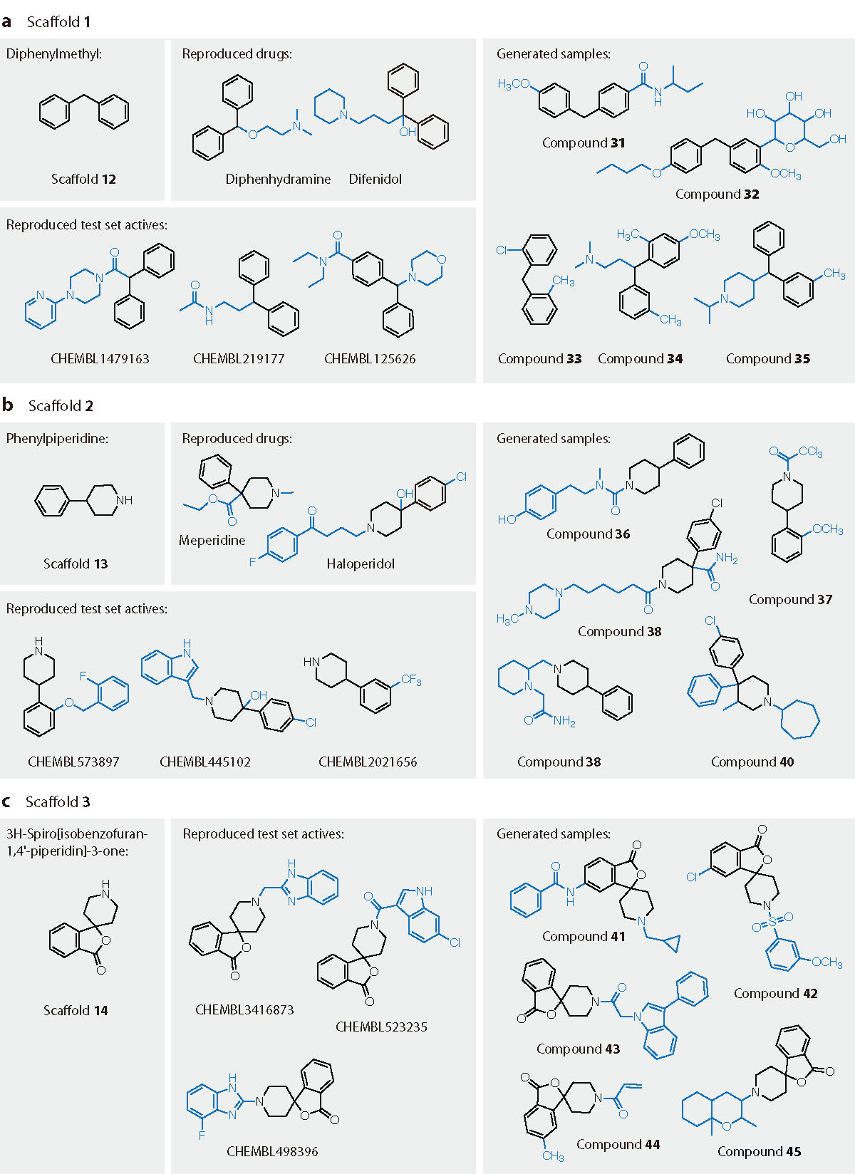
Next, we investigate the ability for the model to reproduce know active molecules against GPCRs (see results in Table LABEL:tab:scaffold). Within 10,000 samples, the model can reproduce 5.17% active molecules and 12.8% known drugs containing scaffold 12, 8.44% active molecules and 25% known drugs containing scaffold 13, as well as 15.9%active molecules containing scaffold 14. Several reproduced drugs are shown in Figure 13. Since the model has no access to those molecules during the training phase, the results above demonstrated good potential for drug discovery based on privileged scaffolds.

Table 2: Case study: privileged scaffolds for GPCRs

	Scaffold 12	Scaffold 13	Scaffold 14
Diversity	0.166	0.187	0.485
Molecular Weight	363.6 (58.1)	384.9 (64.6)	385.3 (38.0)
LogP	4.04 (1.06)	4.01 (1.02)	3.72 (0.698)
QED	0.675 (0.114)	0.708 (0.121)	0.660 (0.0492)
MMD	0.0185	0.00875	0.154
R(actives)	0.0517	0.0844	0.159
R(drugs)	0.128	0.25	-
$P_{s}^{\textrm{valid}}$	0.986	0.974	0.989
$P_{s}^{\textrm{uniq}}$	0.866	0.877	0.454

3.3.7 Analyzing the structural distribution of side chains

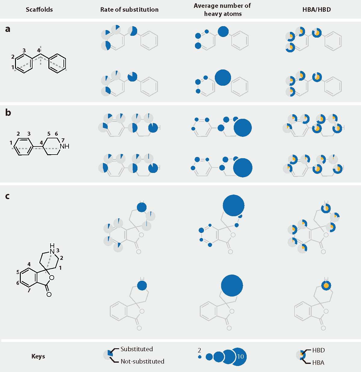
Finally, we investigate the structural distribution of side chains generated by the model. We summarize the result in 14.

The result demonstrated a diversified substitution pattern generated from the model. Note that for scaffold 14, the substitution only happens in location 3 for molecules inside ChEMBL (the reason for the low diversity is discussed in Section 3.3.5). But in the generated molecules, the substitution pattern is much more diverse, demonstrating high generalizability for the model.

Interestingly, it is found that the model adds side-chain to nitrogen atoms more often than other locations. It is also fond the size of side-chain attached to nitrogen atoms tends to be much larger compared with that in other positions. Those observations could be result from a mixed effect of synthetic accessibility and drug-likeness.

Figure 14: The distribution of side chain properties at each location for scaffold 12-14.

3.3.8 Distribution of docking scores

The distribution of docking scores of generated molecules with DRD2 is shown in Figure 15. As demonstrated, the predicted activities of generated samples (orange) are similar to that of the test set molecules (light grey). For scaffold 13 and scaffold 14, the predicted activity against DRD2 for generated samples are significantly higher compared with randomly sampled molecules from ChEMBL, showing that the model is good at utilizing privileged structures for generating bioactive molecules. On the other hand, for scaffold 12, the predicted activities of generated samples could not outperform that of random ChEMBL samples. This may comes from the fact that the bioactivity privilege of scaffold 12 is not as significant compared with 13 and 14, according to the docking result. In fact, scaffold 12 is highly prevalent among molecules in ChEMBL, and could occur in compounds with different targets. This may explain the results for scaffold 12 shown above.

Figure 15: The distribution of docking scores. This plot shows the distribution of docking scores of three sets of molecules (active molecules, generated molecules, test set molecules and random compounds from ChEMBL) for each scaffold (a. scaffold 12, b. scaffold 13 and c. scaffold 14).

4 Conclusion

We proposed a comprehensive solution for scaffold-based drug discovery using deep learning. The model is capable of performing molecular design tasks based on a wide spectrum of scaffold definitions, including BM-scaffolds, cyclic skeletons, as well as scaffolds with specifications on side-chain properties. Evaluation is performed to access the performance of the models. In addition, we choose several privileged scaffolds for GPCRs for the case study, demonstrating the practical value of the model in medicinal chemical problems. We intend to make this tool freely available for academical purposes. Please contact the authors for licensing information.

References

- Hu et al. 2016 Hu, Y.; Stumpfe, D.; Bajorath, J. Computational Exploration of Molecular Scaffolds in Medicinal Chemistry. J Med Chem 2016, 59, 4062–76
- Bemis and Murcko 1996 Bemis, G. W.; Murcko, M. A. The properties of known drugs. 1. Molecular frameworks. J Med Chem 1996, 39, 2887–93
- Barreiro 2015 Barreiro, E. J. Privileged Scaffolds in Medicinal Chemistry; Royal Society of Chemistry: London, 2015
- Varin et al. 2011 Varin, T.; Schuffenhauer, A.; Ertl, P.; Renner, S. Mining for bioactive scaffolds with scaffold networks: improved compound set enrichment from primary screening data. J Chem Inf Model 2011, 51, 1528–38
- Nakagawa et al. 2018 Nakagawa, T.; Miyao, T.; Funatsu, K. Identification of Bioactive Scaffolds Based on QSAR Models. Mol Inform 2018, 37
- Varin et al. 2010 Varin, T.; Gubler, H.; Parker, C. N.; Zhang, J.-H.; Raman, P.; Ertl, P.; Schuffenhauer, A. Compound set enrichment: a novel approach to analysis of primary HTS data. Journal of chemical information and modeling 2010, 50, 2067–2078
- Wilkens et al. 2005 Wilkens, S. J.; Janes, J.; Su, A. I. HierS: hierarchical scaffold clustering using topological chemical graphs. Journal of medicinal chemistry 2005, 48, 3182–3193
- Koch et al. 2005 Koch, M. A.; Schuffenhauer, A.; Scheck, M.; Wetzel, S.; Casaulta, M.; Odermatt, A.; Ertl, P.; Waldmann, H. Charting biologically relevant chemical space: a structural classification of natural products (SCONP). Proc Natl Acad Sci 2005, 102, 17272–7
- Schuffenhauer et al. 2007 Schuffenhauer, A.; Ertl, P.; Roggo, S.; Wetzel, S.; Koch, M. A.; Waldmann, H. The scaffold tree–visualization of the scaffold universe by hierarchical scaffold classification. J Chem Inf Model 2007, 47, 47–58
- Schafer et al. 2017 Schafer, T.; Kriege, N.; Humbeck, L.; Klein, K.; Koch, O.; Mutzel, P. Scaffold Hunter: a comprehensive visual analytics framework for drug discovery. J Cheminform 2017, 9, 28
- LeCun et al. 2015 LeCun, Y.; Bengio, Y.; Hinton, G. Deep learning. Nature 2015, 521, 436–44
- 12 Hu, Z.; Yang, Z.; Salakhutdinov, R.; Xing, E. P. On Unifying Deep Generative Models. International Conference for Learning Representations
- Schneider and Fechner 2005 Schneider, G.; Fechner, U. Computer-based de novo design of drug-like molecules. Nat Rev Drug Discov 2005, 4, 649–63
- Segler et al. 2018 Segler, M. H. S.; Kogej, T.; Tyrchan, C.; Waller, M. P. Generating Focused Molecule Libraries for Drug Discovery with Recurrent Neural Networks. ACS Cent Sci 2018, 4, 120–131
- Gomez-Bombarelli et al. 2018 Gomez-Bombarelli, R.; Wei, J. N.; Duvenaud, D.; Hernandez-Lobato, J. M.; Sanchez-Lengeling, B.; Sheberla, D.; Aguilera-Iparraguirre, J.; Hirzel, T. D.; Adams, R. P.; Aspuru-Guzik, A. Automatic Chemical Design Using a Data-Driven Continuous Representation of Molecules. ACS Cent Sci 2018, 4, 268–276
- Olivecrona et al. 2017 Olivecrona, M.; Blaschke, T.; Engkvist, O.; Chen, H. Molecular de-novo design through deep reinforcement learning. Journal of Cheminformatics 2017, 9, 48
- Weininger 1988 Weininger, D. SMILES, a chemical language and information system. 1. Introduction to methodology and encoding rules. Journal of Chemical Information and Modeling 1988, 28, 31–36
- Li et al. 2018 Li, Y.; Zhang, L.; Liu, Z. Multi-objective de novo drug design with conditional graph generative model. J Cheminform 2018, 10, 33
- Simonovsky and Komodakis 2017 Simonovsky, M.; Komodakis, N. GraphVAE: Towards Generation of Small Graphs Using Variational Autoencoders. arXiv:1610.02920 2017,
- Li et al. 2017 Li, Y.; Vinyals, O.; Dyer, C.; Pascanu, R.; Battaglia, P. Learning Deep Generative Models of Graphs. arXiv:1803.03324 2017,
- 21 You, J.; Ying, R.; Ren, X.; Hamilton, W. L.; Leskovec, J. GraphRNN: Generating Realistic Graphs with Deep Auto-regressive Models. International Conference on Machine Learning
- 22 Jin, W.; Barzilay, R.; Jaakkola, T. Junction Tree Variational Autoencoder for Molecular Graph Generation. International Conference on Machine Learning
- De Cao and Kipf 2018 De Cao, N.; Kipf, T. MolGAN: An implicit generative model for small molecular graphs. arXiv:1805.11973 2018,
- Aumentado-Armstrong 2018 Aumentado-Armstrong, T. Latent Molecular Optimization for Targeted Therapeutic Design. arXiv:1809.02032 2018,
- Zheng et al. 2019 Zheng, S.; Yan, X.; Gu, Q.; Yang, Y.; Du, Y.; Lu, Y.; Xu, J. QBMG: quasi-biogenic molecule generator with deep recurrent neural network. J Cheminform 2019, 11, 5
- Lim et al. 2019 Lim, J.; Hwang, S.-Y.; Kim, S.; Moon, S.; Kim, W. Y. Scaffold-based molecular design using graph generative model. arXiv:1905.13639 2019,
- Gaulton et al. 2012 Gaulton, A.; Bellis, L. J.; Bento, A. P.; Chambers, J.; Davies, M.; Hersey, A.; Light, Y.; McGlinchey, S.; Michalovich, D.; Al-Lazikani, B.; Overington, J. P. ChEMBL: a large-scale bioactivity database for drug discovery. Nucleic Acids Res 2012, 40, D1100–7
- Bickerton et al. 2012 Bickerton, G. R.; Paolini, G. V.; Besnard, J.; Muresan, S.; Hopkins, A. L. Quantifying the chemical beauty of drugs. Nat Chem 2012, 4, 90–8
- Ertl and Schuffenhauer 2009 Ertl, P.; Schuffenhauer, A. Estimation of synthetic accessibility score of drug-like molecules based on molecular complexity and fragment contributions. J Cheminform 2009, 1, 8
- 30 Kingma, D. P.; Welling, M. Auto-encoding variational bayes. International Conference for Learning Representations
- 31 Bowman, S. R.; Vilnis, L.; Vinyals, O.; Dai, A. M.; Jozefowicz, R.; Bengio, S. Generating sentences from a continuous space. SIGNLL Conference on Computational Natural Language Learning
- Higgins et al. 2017 Higgins, I.; Matthey, L.; Pal, A.; Burgess, C.; Glorot, X.; Botvinick, M.; Mohamed, S.; Lerchner, A. beta-VAE: Learning Basic Visual Concepts with a Constrained Variational Framework. ICLR 2017, 2, 6
- Benhenda 2017 Benhenda, M. ChemGAN challenge for drug discovery: can AI reproduce natural chemical diversity? arXiv:1708.08227 2017,
- 34 Li, C.-L.; Chang, W.-C.; Cheng, Y.; Yang, Y.; Póczos, B. Mmd gan: Towards deeper understanding of moment matching network. Advances in Neural Information Processing Systems. pp 2203–2213
- 35 Jiwoong Im, D.; Ma, A. H.; Taylor, G. W.; Branson, K. Quantitatively Evaluating GANs With Divergences Proposed for Training. International Conference on Learning Representations
- 36 Arjovsky, M.; Chintala, S.; Bottou, L. Wasserstein GAN. International Conference on Learning Representations
- Preuer et al. 2018 Preuer, K.; Renz, P.; Unterthiner, T.; Hochreiter, S.; Klambauer, G. Frechet ChemNet Distance: A Metric for Generative Models for Molecules in Drug Discovery. J Chem Inf Model 2018, 58, 1736–1741
- Gower 1971 Gower, J. C. A general coefficient of similarity and some of its properties. Biometrics 1971, 857–871
- Madras 2013 Madras, B. K. History of the discovery of the antipsychotic dopamine D2 receptor: a basis for the dopamine hypothesis of schizophrenia. Journal of the History of the Neurosciences 2013, 22, 62–78
- 40 Chen, X.; Kingma, D. P.; Salimans, T.; Duan, Y.; Dhariwal, P.; Schulman, J.; Sutskever, I.; Abbeel, P. Variational lossy autoencoder. International Conference on Learning Representations
- 41 Kingma, D. P.; Salimans, T.; Jozefowicz, R.; Chen, X.; Sutskever, I.; Welling, M. Improved variational inference with inverse autoregressive flow. Advances in Neural Information Processing Systems. pp 4743–4751