Three-D Safari: Learning to Estimate Zebra Pose, Shape, and
Texture
from Images “In the Wild”
Abstract
We present the first method to perform automatic 3D pose, shape and texture capture of animals from images acquired in-the-wild. In particular, we focus on the problem of capturing 3D information about Grevy’s zebras from a collection of images. The Grevy’s zebra is one of the most endangered species in Africa, with only a few thousand individuals left. Capturing the shape and pose of these animals can provide biologists and conservationists with information about animal health and behavior. In contrast to research on human pose, shape and texture estimation, training data for endangered species is limited, the animals are in complex natural scenes with occlusion, they are naturally camouflaged, travel in herds, and look similar to each other. To overcome these challenges, we integrate the recent SMAL animal model into a network-based regression pipeline, which we train end-to-end on synthetically generated images with pose, shape, and background variation. Going beyond state-of-the-art methods for human shape and pose estimation, our method learns a shape space for zebras during training. Learning such a shape space from images using only a photometric loss is novel, and the approach can be used to learn shape in other settings with limited 3D supervision. Moreover, we couple 3D pose and shape prediction with the task of texture synthesis, obtaining a full texture map of the animal from a single image. We show that the predicted texture map allows a novel per-instance unsupervised optimization over the network features. This method, SMALST (SMAL with learned Shape and Texture) goes beyond previous work, which assumed manual keypoints and/or segmentation, to regress directly from pixels to 3D animal shape, pose and texture. Code and data are available at https://github.com/silviazuffi/smalst.
![[Uncaptioned image]](/html/1908.07201/assets/figures/teaser4.jpg)
1 Introduction
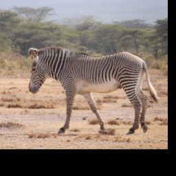
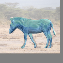
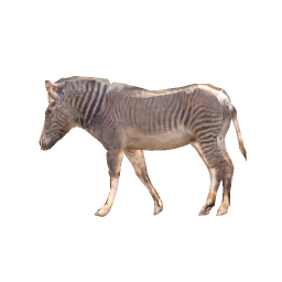
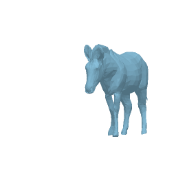
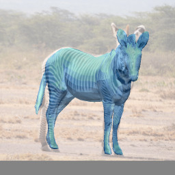
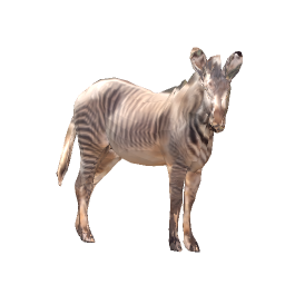
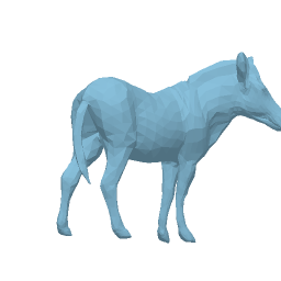
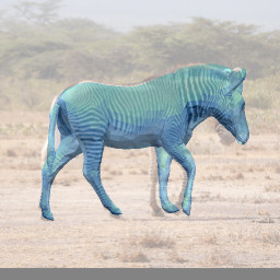
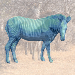
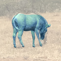
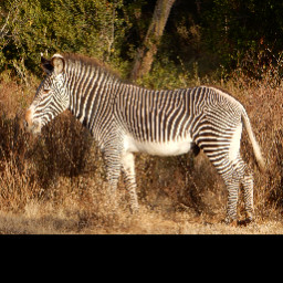
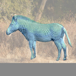
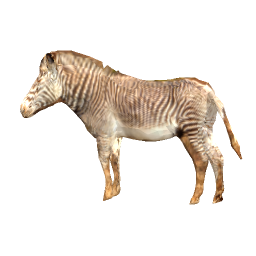
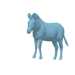
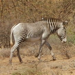
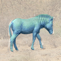
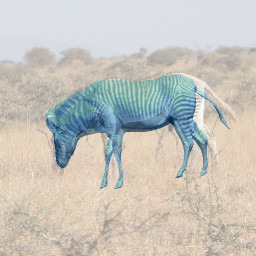
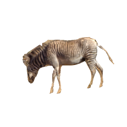
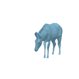
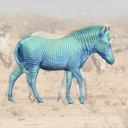
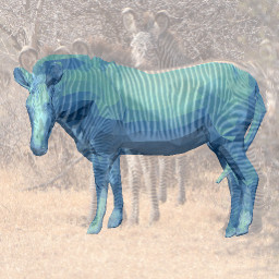
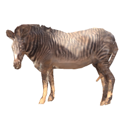
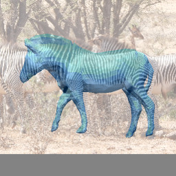
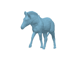
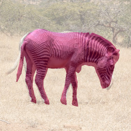
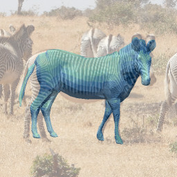
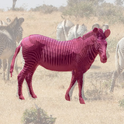
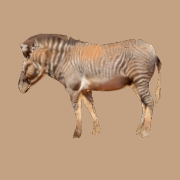
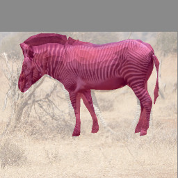
Rapid progress has been made on estimating 3D human pose, shape, and texture from images. Humans are special and, consequently, the amount of effort devoted to this problem is significant. We scan and model the body, label images by hand, and build motion capture systems of all kinds. This level of investment is not possible for every animal species. There are simply too many and the scientific community interested in a particular species may not have the resources for such an effort. This is particularly true of endangered species. We focus on one of the most endangered animal species, the Grevy’s zebra, for which only about 3000 individuals remain [25]. Here we describe a new deep-learning method to regress 3D animal shape, pose, and texture directly from image pixels (Figure 1) that does not require extensive image annotation, addresses the key challenges of animals in the wild, and can scale to large data collections. This provides a new method that can be extended to other species (see Sup. Mat. for results on horses).
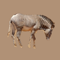
In general, there is very little previous work on estimating animal shape and pose. Existing methods require manual annotation of the test images with keypoints and/or segmentation [33, 34] or clean imaging conditions where automatic segmentation is possible [5].
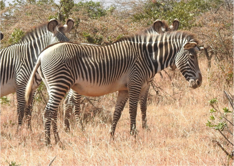
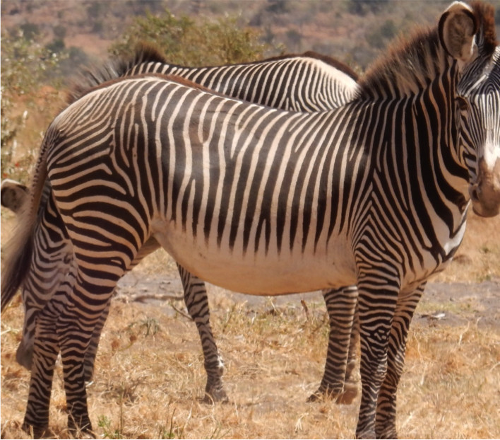
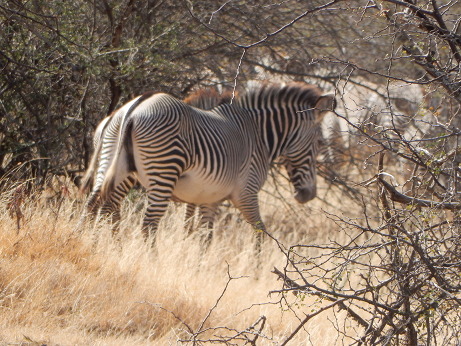
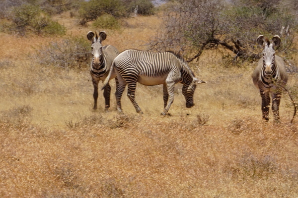
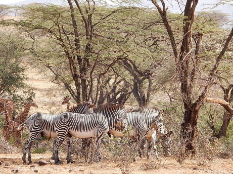
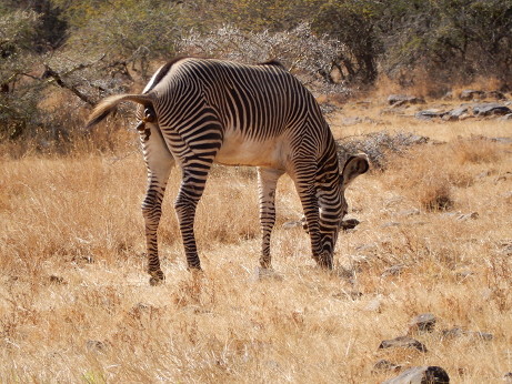
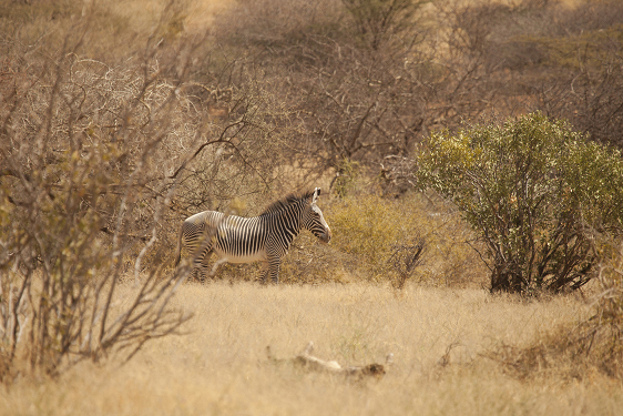
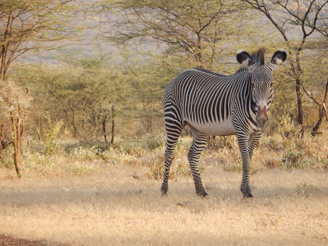
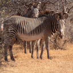
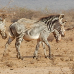
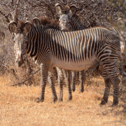
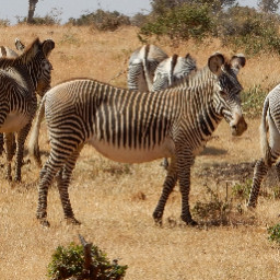
Animals present unique challenges relative to humans (see Figure 2). First, animals often live in environments where their appearance is camouflaged, making bottom-up approaches such as automatic segmentation a challenge. Second, animals like zebras live in herds, where overlapping subjects of similar appearance make reliable keypoint extraction challenging. Third, in comparison to the study of human body pose and shape, the amount of data is limited, particularly for endangered animals, where 3D scanning is infeasible. Thus, although humans and animals are both deformable articulated objects, the lack of training data makes naive application of current deep learning methods that work for humans impractical for animals.
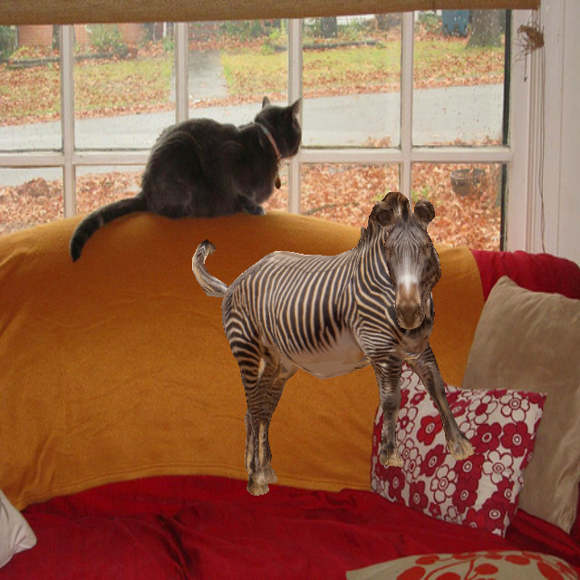
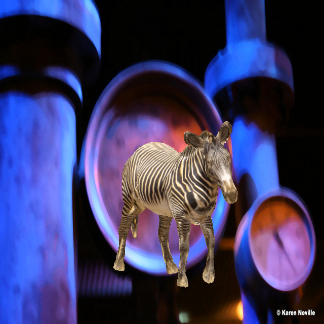
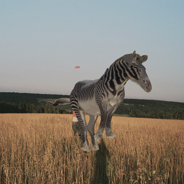
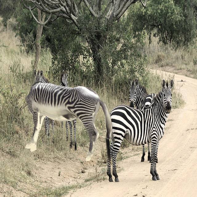
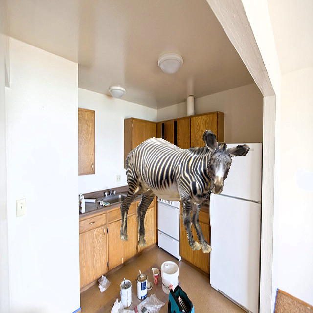
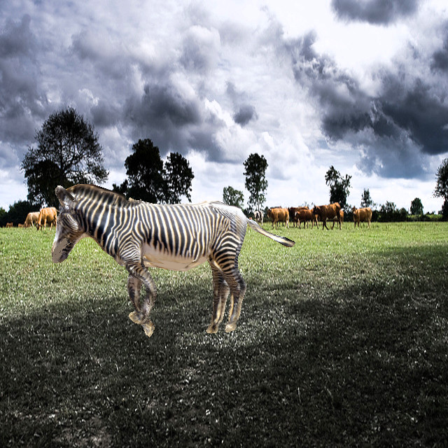
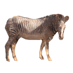
We overcome the lack of data by exploiting synthetic data and an image reconstruction loss using a generative, analysis-by-synthesis, approach. While accurate synthetic human models exist for training, animals models of sufficient quality are rare, particularly for endangered species. A novelty of our approach is that instead of using completely synthetic data, we capture the texture of the animals from real images and render them with variability of background, pose, illumination and camera. This is obtained exploiting the recent SMALR method [33], which allows us to obtain accurate shape, pose, and texture of 10 animals by annotating only about 50 images. From this, adding variations to the subjects, we generate thousands of synthetic training images (Figure 3). We demonstrate that these are realistic enough for our method to learn to estimate body shape, pose and texture from image pixels without any fine-tuning on additional hand-labeled images.
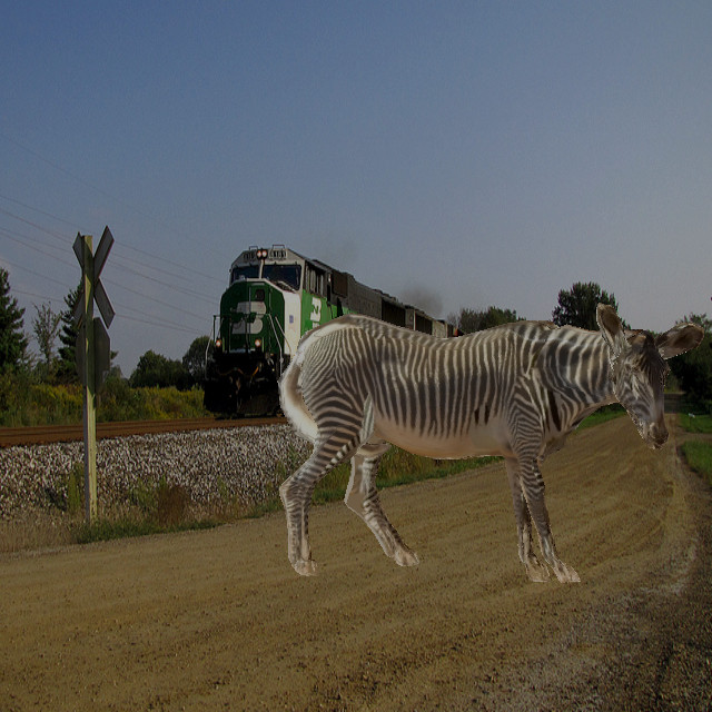
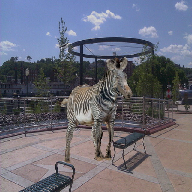
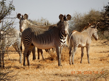
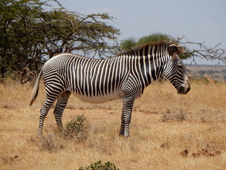
We go beyond previous works in several important ways and our main contributions are as follows. Using a fully generative model of animal shape, appearance, and neural rendering, we use a photometric loss to train a neural network that predicts the 3D pose, shape, and texture map of an animal from a single image. A key novelty of the network is that it links the texture prediction to 3D pose and shape through a shared feature space, such that, in predicting the texture map, the network estimates model parameters for an optimal mapping between image pixels and texture map elements. In order to prevent the network from just learning average texture map colors, inspired by [13], we predict the flow between the image pixels and the texture map. We go beyond [13], however, to deal with an articulated object with a much more complex texture map containing multiple, disconnected regions.
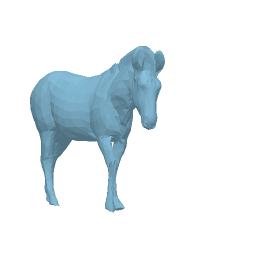
We base our method on a recently introduced 3D articulated shape model of animals, the SMAL model [34], which can represent animals of different shape with a low-dimensional linear model learned from a small set of toys. Instead of relying on the SMAL model shape space, we compute shape variations with a network layer. This corresponds to learning a novel shape space during training and predicting the shape coefficients in this space at test time. We have not seen this sort of neural shape learning before and this is key for endangered species where it would be difficult to build an accurate a priori shape model. Additionally, unlike most human pose estimation methods, we estimate camera focal length. This is important for animals where the elongated shape can result in significant foreshortening. Finally, we also show that, since our network predicts a full texture map, we can exploit the photometric loss to perform a per-instance optimization of the model parameters at test time by searching in the network feature space. By using a background model we are able to refine and obtain more detailed pose and shapes in a fully automatic manner without relying on any segmentation masks at test time. Figure 4 provides an overview of the approach. We call our method SMALST, for SMAL with learned Shape and Texture. We test the approach on a dataset of 200 individual zebra images where we evaluate the method both quantitatively and qualitatively.
2 Previous work
Human 3D Pose and Shape Estimation. The amount of work in the field of 3D human pose estimation is huge; here we review monocular model-based approaches that estimate shape and pose, as they are most related to the goal of this paper. The estimation of 3D pose and shape from monocular images is largely based on low dimensional statistical models of the human body learned from thousands of scans [3, 4, 18]. Currently the most popular model is SMPL [18] and recent work on modeling animals also builds on its formulation. Low-dimensional parametric models are particularly attractive for neural architectures as they can generate high quality meshes from a small number of network-generated parameters. Tan et al. [27] train a network that learns the mapping from silhouettes to pose and shape parameters of the SMPL model. Omran et al. [22] exploit SMPL in conjunction with a bottom-up body part segmentation. Pavlakos et al. [23] estimate 3D body pose and shape of the SMPL model using a two-stage architecture based on 2D keypoints and silhouettes.
Methods focused on humans have the advantage of large datasets of images with ground truth 3D poses captured indoor with mocap systems [9]. We do not have this for animals and indoor imagery does not generalize well to the wild. One way for obtaining approximate 3D pose and shape from outdoor images is to use human annotators. Lassner et al. [15] build a dataset of human-rated high-quality 3D model fits. von Marcard et al. [31] introduce an in-the-wild dataset of human 3D pose and shape obtained by exploiting IMU sensors and video. Alternatively, Varol et al. [29] create SURREAL, a full synthetic dataset of 3D pose and shape. Tung et al. [28] exploit temporal consistency over video frames to train an end-to-end prediction model on images without ground truth 3D pose and shape. Kanazawa et al. [11] exploit adversarial training, which uses decoupled datasets of 2D keypoints and 3D pose and shape to train on in-the-wild images in a weakly-supervised manner.
Model-based methods that capture texture are becoming popular with the goal of creating rigged human avatars. Bogo et al. [6] create 3D models of shape and appearance from RGB-D sequences. Alldieck et al. [2] go further to create 3D textured models with approximate clothing shape from multiple video frames of a subject in a reference pose.
Deep learning methods for human pose and shape estimation combine powerful 2D joint detectors, accurate body part segmentations, large datasets of human 3D pose, and an expressive articulated 3D shape model. None of the previous work exploits appearance, likely because it varies so much due to clothing. For birds, not humans, Kanazawa et al. [13] learn a generative model of appearance by modeling the way surface colors are mapped from the image to a texture map. In our work we explore this approach to appearance modeling in conjunction with a SMPL-style model of animals with the intuition that learning to predict texture helps in the task of pose and shape recovery.
Animals Pose and Shape Estimation. Animals are presented in many object-recognition datasets where methods for bounding box detection, recognition, and instance segmentation are common [8]. There is very little work, however, on detecting 3D animal shape and pose. The seminal work on this from Cashman and Fitzgibbon [7] shows how to estimate the shape of dolphins from monocular images. Ntouskos et al. [21] model articulated animals as a collection of 3D primitives that they estimate from segmented images. Vincente and Agapito [30] show how to build a rough giraffe shape from two views. Kanazawa et al. [12] learn deformation models for cats and horses. Kanazawa et al. [13] predict 3D shape and texture of birds from images, without assuming a template model of the bird’s 3D shape, but they do not model pose. Methods based on video have potentially more information about animal shape at their disposal. Reinert et al. [24] show the extraction of a rough animal shape from video in terms of generalized cylinders. They also recover a texture map from one video frame.
In contrast to humans, none of the previous approaches is based on 3D animal models learned from scans, therefore they lack realism and fine detail. Moreover, previous work estimates the 3D shape of a single animal; none address the problem of capturing shape for a large number of subjects of the same species with variable body shape.
Zuffi et al. [34] introduced the SMAL model, a 3D articulated shape model of animals, that can represent inter and intra species shape variations. They train the model from scans of toys, which may not exist for endangered species or may not be accurate. They go further in [33] to fit the model to multiple images, while allowing the shape to deform to fit to the individual shape of the animals. This allows them to capture shape outside of the SMAL shape space, increasing realism and generalization to unseen animal shapes. Unfortunately, the method is based on manually extracted silhouettes and keypoint annotations. More recently, Biggs et al. [5] fit the SMAL model to images automatically by training a joint detector on synthetically generated silhouettes. At inference time, their method requires accurate segmentation and is not robust to occlusion.
In biology, animal tracking is extremely important and many tools exist. Recently deep learning methods have been applied to help solving the feature tracking problem. Mathis et al. [20] use deep learning to track animal keypoints defined by a user on infrared images captured in the lab. They show applications to rodents, bees and other small animals. So far, no methods address the shape and pose estimation problem we tackle here.
3 Approach
We formulate the problem of estimating the 3D pose and shape of zebras from a single image as a model-based regression problem, where we train a neural network to predict 3D pose, shape and texture for the SMAL model.
An important aspect of our approach is that we rely on a digitally generated dataset to train our network. While the quality of synthetic image generation has dramatically improved thanks to advancements in computer graphics rendering and 3D modeling approaches, such synthetic data are expensive to obtain and insufficient in terms of variation in shape and appearance. Unlike faces, where the community has developed realistic generative models of shape and appearance from a large amount of high quality 3D scans, no convincing generative models of 3D animals exist.
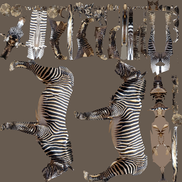
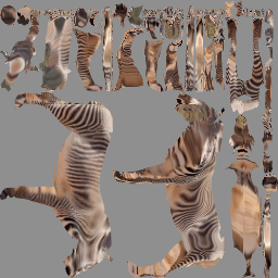
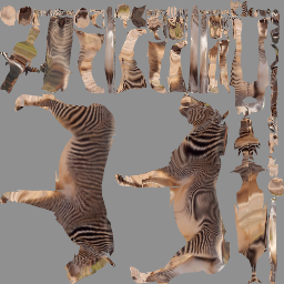
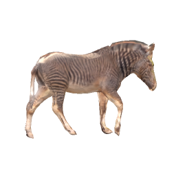
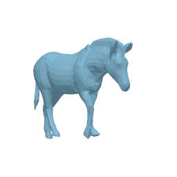
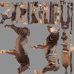
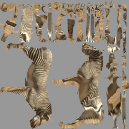
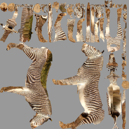
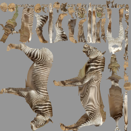
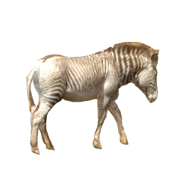
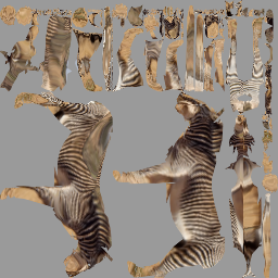
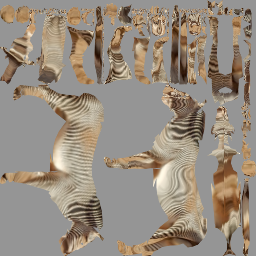
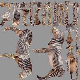
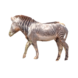
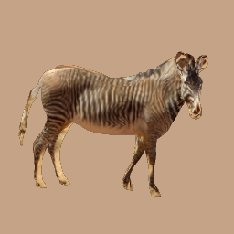
Instead of relying on synthetic data that is not sufficiently realistic for representing animals, we capture appearance from real images and use this data to render realistic samples with pose, shape and background variation. This approach of mixing real and synthetic is not novel: Alhaija et al. [1] use synthetic cars in a real scene; here we do the opposite: use real subjects against random backgrounds. We use the SMALR method [33] to create instance-specific SMAL models from images with a captured texture map (see an example in Figure 5 left). We animate and render such models to create our digital training set.
3.1 SMAL model
The SMAL model is a function of shape , pose and translation . is a vector of the coefficients of the learned PCA shape space, is the relative rotation, expressed with Rodrigues vectors, of the joints in the kinematic tree, and is the global translation applied to the root joint. Unlike [34], which uses joints, we segment and add articulation to the ears, obtaining a model with body parts. The SMAL function returns a 3D mesh, where the model template is shaped by , articulated by and shifted by . Formally, let be a row vector of shape variables, then vertices of a subject-specific shape in the reference T-pose are computed as:
| (1) |
where represents the vertices of the SMAL model template and is a matrix of deformation vectors. In this work we focus on an animal in the Equine family, thus the template is the shape that corresponds to the mean horse in the original SMAL model. Given a set of pose variables and global translation , the model generates 3D mesh vertices in the desired pose by articulating with linear blend skinning.
SMALR. Zuffi et al. [33] show that aligning the SMAL model to images and then allowing the model vertices to deviate from the linear shape model can create realistic textured 3D models of unseen animals from images. The method is based on an initial stage where SMAL is fitted to a set of images of the same animal from different views and poses, obtaining an estimation of global shape parameters , per image translation , pose , and camera focal length . In a refinement step, shape parameters, translations, poses and cameras are held fixed, but the model shape is allowed to change through a set of displacement vectors:
| (2) |
where the superscript SMALR indicates that the displacement vector dv is obtained with the SMALR method.
3.2 Digital dataset
We created a computer generated dataset of 12850 RGB images of single zebras. We applied SMALR to a set of 57 images of Grevy’s zebras creating models for 10 different subjects. For each zebra model we generated random images that differ in background, shape, pose, camera, and appearance. Models are rendered with OpenDR [17]. Examples of the images are in Figure 3, top.
Pose variation. For each zebra model we generated 1000 images with different poses obtained by sampling a multivariate Gaussian distribution over the 3D Rodrigues vectors that describe pose. The sampling distribution is learned from the 57 poses obtained with SMALR and a synthetic walking sequence. We also add, for each zebra model, about 285 images obtained by adding noise to the 57 poses. We also add noise to the reference animal translation, that we set at . Changing depth varies the size of the animal as we use perspective projection.
Appearance variation. In order to vary the appearance of the zebras, we apply a white-balance algorithm to the textures, doubling the number of texture maps, while on the generated images we randomly add noise to the brightness, hue and saturation levels. Moreover, we also randomly add lighting to the rendered scene. We generate images with random backgrounds by sampling background images from the COCO dataset [16].
Shape and size variation. We increase the variability of the zebra shapes by adding noise to the shape variables (we use 20 shape variables). In addition to size variations due to depth, we add size variation by adding noise to the reference camera, which has a reference focal length .
Images are created with size . For each image we also compute the texture uv-flow that represents the mapping between image pixels and textels, and can be interpreted as the flow between the image and the texture map. For each image we save the following annotation data: texture map , texture uv-flow , silhouette , pose , global translation , shape variables , vertex displacements , landmark locations . We use a total of 28 surface landmarks, placed at the joints, on the face, ears and tail tip. These are defined only once on the 3D model template.
3.3 Real datasets
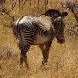
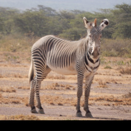
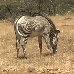
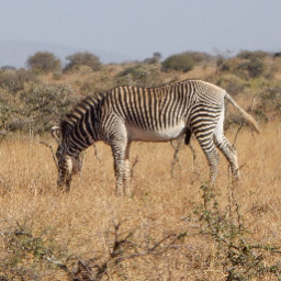
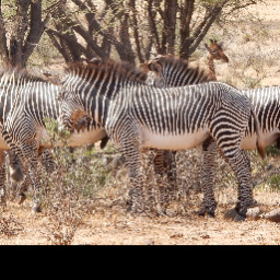
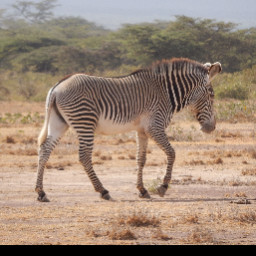
For evaluation, we have collected a new dataset of images of Gravy’s zebra captured in Kenya with pre-computed bounding boxes. Examples of the images are in Figure 3, bottom. We selected a set of 48 images of zebras that were not used to create the digital dataset, and we annotated them for 2D keypoints. We used this as validation set. We then selected 100 images as our test set, also avoiding zebras from the two sets above. For evaluation, we manually generated the segmentation mask for this set of images, and annotated the 2D keypoints. We mirror the images in order to double the test set data.
3.4 Method
We design a network to regress a texture map , dv, 3D pose , translation and focal length variables from an input image. We implemented the SMAL model in PyTorch. The vertex displacements from the template are not computed as in SMAL (see Equation 1), but are estimated from the regression network. Formally:
| (3) |
where dv is a displacement vector generated as output of a linear layer. Consequently, given ground truth shapes from Equation 2, we define ground truth vertex displacements for network training as: . We use the Neural Mesh Renderer (NMR) [14] for rendering the model and perspective projection.

The regression network is illustrated in Figure 4. The encoder is composed of a Resnet 50 module that computes image features for an image of size . At training time the input image is a noisy bounding box computed given the ground truth segmentation mask. Ground truth values of translation and camera focus are modified accordingly when computing the bounding box. At test time the input image is a pre-computed bounding box of the animal. The Resnet module is followed by a convolutional layer with group normalization and leaky ReLU. The output of this layer is of size 2048. We then add 2 fully connected layers, each of them composed by a linear layer, batch normalization and leaky ReLU. We obtain as output a set of 1024 features. From this set of features, we add independent layers that predict texture, shape, 3D pose, translation and camera focus.
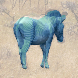
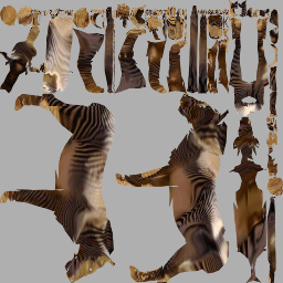
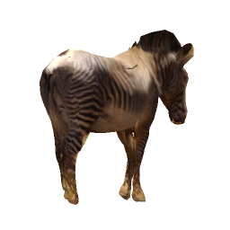
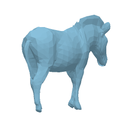
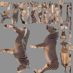
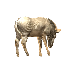
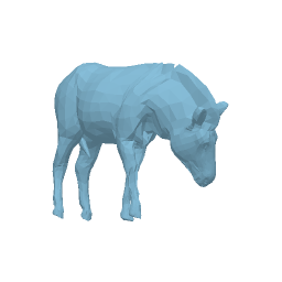
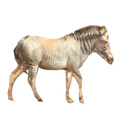
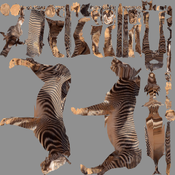
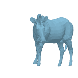
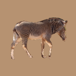
Texture prediction. The texture prediction module is inspired by the work of Kanazawa et al. [13]. While [13] explores texture regression on a simple texture map that corresponds to a sphere, quadrupeds, like zebras, have a more complicated surface and texture map layout. We therefore predict the texture map as a collection of 4 sub-images that we then stitch together. We found this to work better than directly predicting the full texture map, probably because, given the complexity of the articulated model, the network has difficulty with the spatial discontinuities in the texture map. We cut the texture map (that has size ) into 4 regions illustrated in Figure 5. For each sub-image we define an encoder and decoder. Each encoder outputs a feature map, where H and W are a reduction of 32 of the size of the sub-image, and is composed of 2 fully connected layers. The decoders are composed of a set of convolutional layers and a final tanh module. The output of the decoders is stitched to create a full uv-flow map, that encodes which image pixels correspond to pixels in the texture map.

Shape prediction. The shape prediction module is composed of a fully connected layer that outputs shape features , and a linear layer that predicts vertex deformations:
| (4) |
where is a bias term. is initialized with the SMAL blendshapes (see Equation 1). We want to represent the shapes with a linear model that is more expressive than SMAL, therefore we seek to optimize the shape blendshapes through the network. In order to limit the number of network parameters, we exploit the symmetry of the SMAL model and predict only half of the mesh vertices.
Pose prediction. The pose prediction module is a linear layer that outputs a vector of 3D poses as relative joint angles, expressed as Rodrigues vectors. The pose vector is of size as we use body joints.
Translation prediction. The translation prediction module is composed of two linear layers that predict translation in the camera frame and depth independently: , , , where are the outputs of the prediction layer, as in the synthetic dataset. We add to the coordinate due to the distribution of the ground truth values in the training set.
Camera prediction. The camera prediction layer predicts the focal length of the perspective camera. Since we also predict the depth in the network, this parameter can be redundant; however we have found empirically that it allows better model fits to images. The camera focal length is obtained as , where is the output of the prediction layer and .
3.5 3D pose, shape and texture estimation
We train the network to minimize the loss:
| (5) |
where: is the mask, is the mask loss, defined as the L1 loss between and the predicted mask. is the 2D keypoint loss, defined as the MSE loss between and the projected 3D keypoints defined on the model vertices. is the camera loss, defined as the MSE loss between and predicted focal length. is the image loss, computed as the perceptual distance [32] between the masked input image and rendered zebra. is the MSE loss between and predicted 3D poses, computed as geodesic distance [19]. is the translation loss, defined as the MSE between and predicted translation. is the shape loss, defined as the MSE between and predicted dv. is the uv-flow loss, defined as the L1 loss between and the predicted uv-flow. Note that the ground truth uv-flows are necessarily incomplete because, from one image, we can only assign a partial texture map. When generating the digital dataset we also compute visibility masks for the uv-flow, that we exploit for computing the loss only on the visible textels. is the L1 loss between the and the predicted texture map. is a texture loss term that encourages the uv-flow to pick colors from the foreground region (see [13]). This term is consistently applied to the full texture. Each loss is associated with a weight. Note that we include both a loss on the model parameters and a loss on silhouettes and projected keypoints. Similar to Pavlakos et al. [23], we observed that a per-vertex loss improves training compared with naive parameter regression. The network is implemented in PyTorch.

3.6 Per-instance optimization
The prediction of the texture map allows us to perform an unsupervised per-instance optimization exploiting the learned feature space and a photometric loss. Methods that also exploit photometric loss often are assisted by a segmentation [10], where the loss is computed only in the foreground region. In this work we do not assume any segmentation is available at test time, instead we render a full image prediction, which requires building a background model [26]. We estimate an average background color exploiting the manual segmentations of the images used to build the SMALR models for training. Given an input image, we run the regression network and then perform a per-instance optimization where we keep the network layers fixed and optimize over the feature space variables (Figure 4 dotted line). In this way we exploit the correlation between variables learned by the network. During optimization we minimize the following loss:
| (6) |
where is the photometric loss, computed as the perceptual distance [32] between input image and image prediction. and are the initialization values for focal length and translation estimated with the network, respectively.
4 Experiments
Direct regression from the image. We train two networks: a full network and one without the texture prediction module, which is therefore trained without the uv-flow loss , the image loss , and the texture map losses and . We train both networks for a budget of 200 epochs, and retain the networks that performed best on the validation set. We use the Adam optimizer with a learning rate of and momentum of .
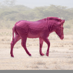
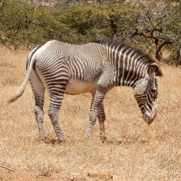
We run the prediction network on the set of 200 annotated test images; see Figure 6 for representative results. Table 1 reports the average PCK error for the predicted 2D keypoints at two thresholds for the feed-forward prediction (F) and for the network without texture prediction (G). For comparison with previous work we fit the SMAL model to the testset using the manual segmentations and keypoint annotations (A). We also evaluate the performance on a synthetic dataset (B). To illustrate robustness, we perform an experiment adding noise to the input bounding boxes (H). To quantify the accuracy of the shape estimation, we compute an overlap score as intersection over union of the manual image segmentations and predicted animal mask.
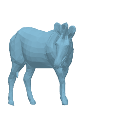
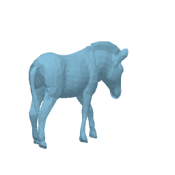
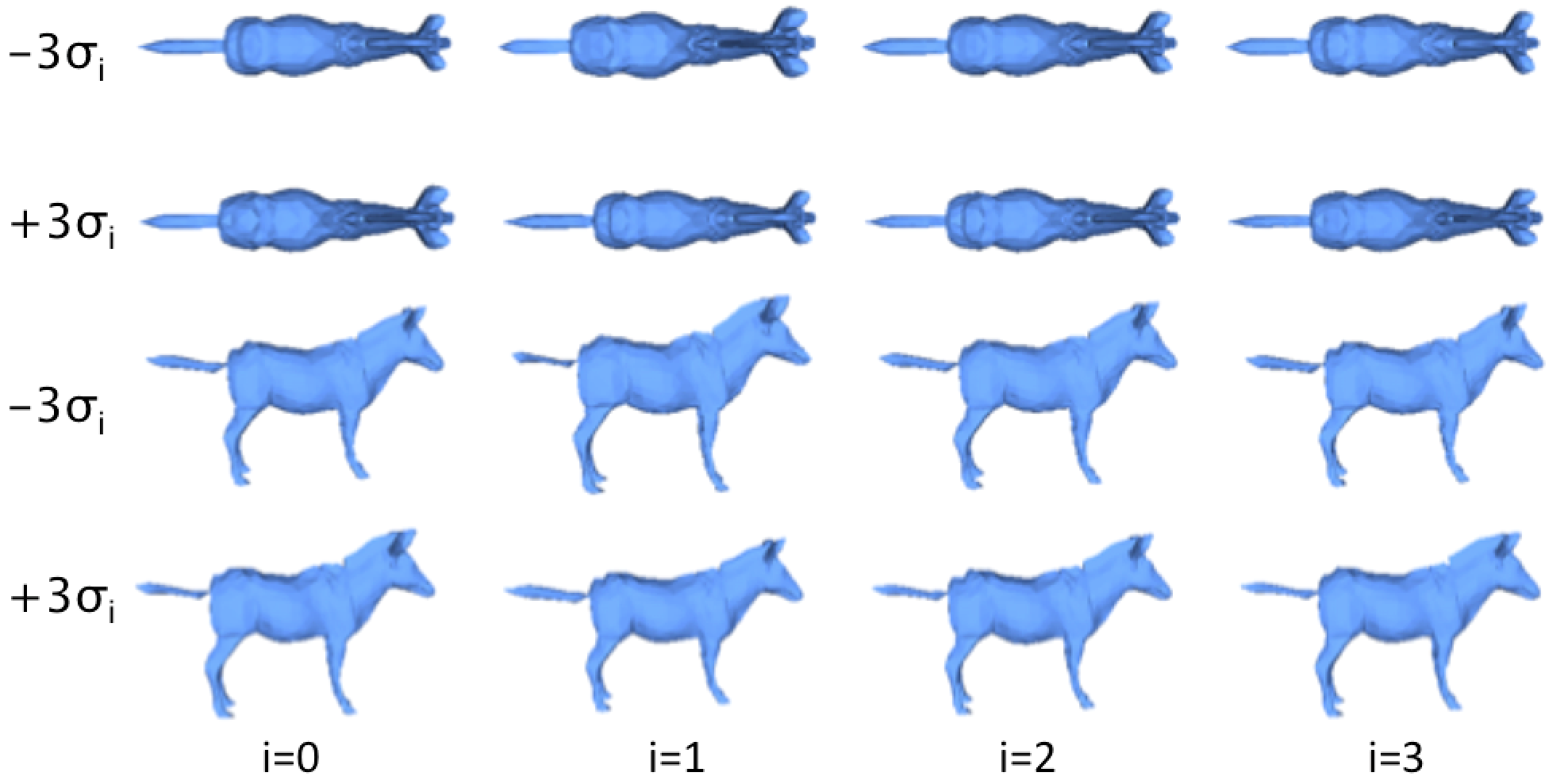
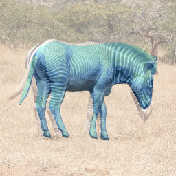
In order to visualize the variability of the estimated shape we computed the variance of the shape features obtained on the test set (see Equation 4) and look at the deformations that are associated with the features with maximum variance. In Figure 7 (top) we show in the odd rows, and in the even rows, where is the standard deviation of the shape feature and is a row in the learned matrix (Equation 4). In order to visualize the difference between the initial SMAL shape space and the shape space learned from the network, Figure 7 (bottom) shows the mean shape of the network model (blue) obtained by adding the bias to the SMAL template, the SMAL template (pink) and the average of the SMALR meshes used to create the training set (green).

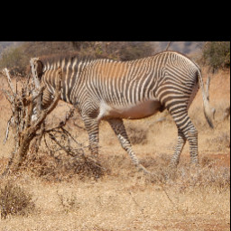
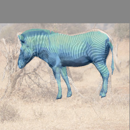
Per-instance optimization. We run per-instance optimization on the whole test set. We optimize over a budget of 120 epochs, and retain the solution with lowest photometric loss. Table 1 shows the performance of the optimization (C). Figure 8 shows some examples. For comparison, we also perform per-instance optimization over the model variables (D).
| Method | PCK@0.05 | PCK@0.1 | IoU |
|---|---|---|---|
| (A) SMAL (gt kp and seg) | 92.2 | 99.4 | 0.463 |
| (B) feed-forward on synthetic | 80.4 | 97.1 | 0.423 |
| (C) opt features | 62.3 | 81.6 | 0.422 |
| (D) opt variables | 59.2 | 80.6 | 0.418 |
| (E) opt features bg img | 59.7 | 80.5 | 0.416 |
| (F) feed-forward pred. | 59.5 | 80.3 | 0.416 |
| (G) no texture | 52.3 | 76.2 | 0.401 |
| (H) noise bbox | 58.7 | 79.9 | 0.415 |

5 Conclusion
We have presented the first study of automatic 3D pose, shape and appearance capture of animals from a single image acquired “in-the-wild”. Traditionally the focus of computer vision research has been the human body: dealing with wild animals presents new technical challenges. We overcome the lack of training data by creating a digital dataset that combines real appearance with synthesized pose, shape and background. We remove the need for keypoint detection or segmentations by training an end-to-end network to directly regress 3D pose, shape, camera, global translation and texture from an image. We have shown that predicting texture maps helps to recover more accurate pose and shape. Moreover we have shown that, thanks to the predicted texture map, we can improve results by performing per-instance network-based optimization over the encoder features by exploiting a photometric loss. In this work we have focused on the Grevy’s zebra, but our approach is general and can be applied to other animals or humans.
Acknowledgement. AK is supported by BAIR sponsors. TBW is supported by NSF grant III-1514126.
Disclosure. MJB has received research gift funds from Intel, Nvidia, Adobe, Facebook, and Amazon. While MJB is a part-time employee of Amazon, his research was performed solely at MPI. He is also an investor in Meshcapde GmbH.
References
- [1] Hassan Abu Alhaija, Siva Karthik Mustikovela, Lars Mescheder, Andreas Geiger, and Carsten Rother. Augmented reality meets deep learning for car instance segmentation in urban scenes. In Proceedings of the British Machine Vision Conference 2017, Sept. 2017.
- [2] Thiemo Alldieck, Marcus Magnor, Weipeng Xu, Christian Theobalt, and Gerard Pons-Moll. Video based reconstruction of 3d people models. In IEEE Conference on Computer Vision and Pattern Recognition (CVPR), June 2018.
- [3] Brett Allen, Brian Curless, Brian Curless, and Zoran Popović. The space of human body shapes: Reconstruction and parameterization from range scans. In ACM SIGGRAPH 2003 Papers, SIGGRAPH ’03, pages 587–594, New York, NY, USA, 2003. ACM.
- [4] Dragomir Anguelov, Praveen Srinivasan, Daphne Koller, Sebastian Thrun, Jim Rodgers, and James Davis. SCAPE: Shape Completion and Animation of PEople. ACM Trans. Graph. (Proc. SIGGRAPH, 24(3):408–416, 2005.
- [5] Benjamin Biggs, Thomas Roddick, Andrew Fitzgibbon, and Roberto Cipolla. Creatures great and SMAL: Recovering the shape and motion of animals from video. In ACCV, 2018.
- [6] Federica Bogo, Michael J. Black, Matthew Loper, and Javier Romero. Detailed full-body reconstructions of moving people from monocular RGB-D sequences. In International Conference on Computer Vision (ICCV), pages 2300–2308, Dec. 2015.
- [7] Tom J. Cashman and Andrew W. Fitzgibbon. What shape are dolphins? building 3d morphable models from 2d images. IEEE Transactions on Pattern Analysis and Machine Intelligence, 35(1):232–244, Jan 2013.
- [8] Kaiming He, Georgia Gkioxari, Piotr Dollár, and Ross Girshick. Mask R-CNN. In Proceedings of the International Conference on Computer Vision (ICCV), 2017.
- [9] Catalin Ionescu, Dragos Papava, Vlad Olaru, and Cristian Sminchisescu. Human3.6m: Large scale datasets and predictive methods for 3d human sensing in natural environments. IEEE Transactions on Pattern Analysis and Machine Intelligence, 36(7):1325–1339, jul 2014.
- [10] Michael Janner, Jiajun Wu, Tejas D. Kulkarni, Ilker Yildirim, and Josh Tenenbaum. Self-supervised intrinsic image decomposition. In NIPS, pages 5938–5948, 2017.
- [11] Angjoo Kanazawa, Michael J. Black, David W. Jacobs, and Jitendra Malik. End-to-end recovery of human shape and pose. In Computer Vision and Pattern Regognition (CVPR), 2018.
- [12] Angjoo Kanazawa, Shahar Kovalsky, Ronen Basri, and David W. Jacobs. Learning 3D deformation of animals from 2D images. In Eurographics, 2016.
- [13] Angjoo Kanazawa, Shubham Tulsiani, Alexei A. Efros, and Jitendra Malik. Learning category-specific mesh reconstruction from image collections. In ECCV, 2018.
- [14] Hiroharu Kato, Yoshitaka Ushiku, and Tatsuya Harada. Neural 3d mesh renderer. In 2018 IEEE Conference on Computer Vision and Pattern Recognition, CVPR 2018, Salt Lake City, UT, USA, June 18-22, 2018, 2018.
- [15] Christoph Lassner, Javier Romero, Martin Kiefel, Federica Bogo, Michael J. Black, and Peter V. Gehler. Unite the people: Closing the loop between 3d and 2d human representations. In Proceedings IEEE Conference on Computer Vision and Pattern Recognition (CVPR) 2017, Piscataway, NJ, USA, July 2017. IEEE.
- [16] Tsung-Yi Lin, Michael Maire, Serge Belongie, James Hays, Pietro Perona, Deva Ramanan, Piotr Dollár, and C. Lawrence Zitnick. Microsoft coco: Common objects in context. In David Fleet, Tomas Pajdla, Bernt Schiele, and Tinne Tuytelaars, editors, Computer Vision – ECCV 2014, pages 740–755, Cham, 2014. Springer International Publishing.
- [17] Matthew Loper and Michael J. Black. OpenDR: An approximate differentiable renderer. In European Conf. on Computer Vision (ECCV), pages 154–169, 2014.
- [18] Matthew Loper, Naureen Mahmood, Javier Romero, Gerard Pons-Moll, and Michael J. Black. SMPL: A skinned multi-person linear model. ACM Trans. Graphics (Proc. SIGGRAPH Asia), 34(6):248:1–248:16, Oct. 2015.
- [19] Siddharth Mahendran, Haider Ali, and René Vidal. 3d pose regression using convolutional neural networks. In 2017 IEEE Conference on Computer Vision and Pattern Recognition Workshops (CVPRW), pages 494–495, July 2017.
- [20] Alexander Mathis, Pranav Mamidanna, Kevin M. Cury, Taiga Abe, Venkatesh N. Murthy, Mackenzie Weygandt Mathis, and Matthias Bethge. Deeplabcut: markerless pose estimation of user-defined body parts with deep learning. Nature Neuroscience, 21(9):1281–1289, 2018.
- [21] Valsamis Ntouskos, Marta Sanzari, Bruno Cafaro, Federico Nardi, Fabrizio Natola, Fiora Pirri, and Manuel Ruiz. Component-wise modeling of articulated objects. In International Conference on Computer Vision (ICCV), December 2015.
- [22] Mohamed Omran, Christoph Lassner, Gerard Pons-Moll, Peter Gehler, and Bernt Schiele. Neural body fitting: Unifying deep learning and model based human pose and shape estimation. In International Conference on 3D Vision (3DV), sep 2018.
- [23] Georgios Pavlakos, Luyang Zhu, Xiaowei Zhou, and Kostas Daniilidis. Learning to estimate 3d human pose and shape from a single color image. In 2018 IEEE Conference on Computer Vision and Pattern Recognition, CVPR 2018, Salt Lake City, UT, USA, June 18-22, 2018, pages 459–468, 2018.
- [24] Bernhard Reinert, Tobias Ritschel, and Hans-Peter Seidel. Animated 3D creatures from single-view video by skeletal sketching. In GI’16: Proc. of the 42nd Graphics Interface Conference, 2016.
- [25] Daniel I. Rubenstein, Jason Parham, Charles V. Stewart, Tanya Y. Berger-Wolf, Jason Holmberg, Jon Crall, Belinda L. Mackey, Sheila Funnel, Kasmira Cockerill, Zeke Davidson, Lizbeth Mate, Cosmas Nzomo, Rosemary Warungu, Dino Martins, Vincent Ontita, Joy Omulupi, Jennifer Weston, George Anyona, Geoffrey Chege, David Kimiti, Kaia Tombak, Andrew Gersick, and Nancy Rubenstein. The state of kenya’s grevy’s zebras and reticulated giraffes: Results of the great grevy’s rally 2018. Report to the Kenya Wildlife Service, June 2018.
- [26] Sandro Schönborn, Bernhard Egger, Andreas Forster, and Thomas Vetter. Background modeling for generative image models. Comput. Vis. Image Underst., 136(C):117–127, July 2015.
- [27] Vince Tan, Ignas Budvytis, and Roberto Cipolla. Indirect deep structured learning for 3d human body shape and pose prediction. In British Machine Vision Conference 2017, BMVC 2017, London, UK, September 4-7, 2017, 2017.
- [28] Hsiao-Yu Tung, Hsiao-Wei Tung, Ersin Yumer, and Katerina Fragkiadaki. Self-supervised learning of motion capture. In Advances in Neural Information Processing Systems, pages 5242–5252, 2017.
- [29] Gül Varol, Javier Romero, Xavier Martin, Naureen Mahmood, Michael J. Black, Ivan Laptev, and Cordelia Schmid. Learning from synthetic humans. In Proceedings IEEE Conference on Computer Vision and Pattern Recognition (CVPR) 2017, Piscataway, NJ, USA, July 2017. IEEE.
- [30] Sara Vicente and Lourdes Agapito. Balloon shapes: Reconstructing and deforming objects with volume from images. In Conference on 3D Vision-3DV, 2013.
- [31] Timo von Marcard, Roberto Henschel, Michael J. Black, Bodo Rosenhahn, and Gerard Pons-Moll. Recovering accurate 3D human pose in the wild using IMUs and a moving camera. In European Conference on Computer Vision (ECCV), volume Lecture Notes in Computer Science, vol 11214, pages 614–631. Springer, Cham, Sept. 2018.
- [32] Richard Zhang, Phillip Isola, Alexei A Efros, Eli Shechtman, and Oliver Wang. The unreasonable effectiveness of deep features as a perceptual metric. In CVPR, 2018.
- [33] Silvia Zuffi, Angjoo Kanazawa, and Michael J. Black. Lions and tigers and bears: Capturing non-rigid, 3D, articulated shape from images. In IEEE Conference on Computer Vision and Pattern Recognition (CVPR). IEEE Computer Society, 2018.
- [34] Silvia Zuffi, Angjoo Kanazawa, David Jacobs, and Michael J. Black. 3D menagerie: Modeling the 3D shape and pose of animals. In Proceedings IEEE Conference on Computer Vision and Pattern Recognition (CVPR) 2017, pages 5524–5532, Piscataway, NJ, USA, July 2017. IEEE.