Damping Mechanisms of the Solar Filament Longitudinal Oscillations in Weak Magnetic Field

Abstract

Longitudinal oscillations of solar filament have been investigated via numerical simulations continuously, but mainly in one dimension (1D), where the magnetic field line is treated as a rigid flux tube. Whereas those one-dimensional simulations can roughly reproduce the observed oscillation periods, implying that gravity is the main restoring force for filament longitudinal oscillations, the decay time in one-dimensional simulations is generally longer than in observations. In this paper, we perform a two-dimensional (2D) non-adiabatic magnetohydrodynamic simulation of filament longitudinal oscillations, and compare it with the 2D adiabatic case and 1D adiabatic and non-adiabatic cases. It is found that, whereas both non-adiabatic processes (radiation and heat conduction) can significantly reduce the decay time, wave leakage is another important mechanism to dissipate the kinetic energy of the oscillating filament when the magnetic field is weak so that gravity is comparable to Lorentz force. In this case, our simulations indicate that the pendulum model might lead to an error of $\sim$100% in determining the curvature radius of the dipped magnetic field using the longitudinal oscillation period when the gravity to Lorentz force ratio is close to unity.

1 Introduction

Solar filaments, or called prominences when appearing above the solar limb, are cold dense plasma concentrations embedded in the hot tenuous corona. In the early era when the spatial resolution of observations was not high, filaments seem to be static, hence they were thought to be held in equilibrium with the Lorentz force balancing the gravity. Therefore, it was proposed that the local magnetic field of filaments should have a dipped configuration, either of a normal-polarity type (Kippenhahn & Schlüter, 1957) or inverse-polarity type (Kuperus & Raadu, 1974). After the dynamic features were discovered, e.g., the counterstreamings (Zirker et al., 1998), it was suggested that a dipped magnetic configuration is not necessary, and a prominence could be be a completely dynamic structure, with existing plasma draining down and new plasma replenishing it (Karpen et al., 2001). Such a possibility was validated in some observations (Wang, 1999; Zou et al., 2016).

Even in the case with magnetic dips, some filaments are never static. They oscillate in response to any perturbations, which are ubiquitous in the solar atmosphere. From the physical point of view, filament oscillations can be divided into transverse and longitudinal modes (Shen et al., 2014; Zhang et al., 2017; Arregui et al., 2018), where the oscillation direction is perpendicular and parallel to the local magnetic field, respectively. Similar to other oscillating phenomena, filament oscillations, characterized by oscillation period and decay time, can also be utilized to estimate some physical parameters, mainly the magnetic field. This is called prominence seismology (Arregui et al., 2018). Hence, it is important to understand what determines the oscillation period and what determines the decay time.

Filament longitudinal oscillations were first reported by Jing et al. (2003), and in fact, the counterstreamings existing in many solar filaments might be due to longitudinal oscillations of filament threads (Lin et al., 2003), although the counterstreamings in some filaments are alternating unidirectional flows (Zou et al., 2017) or are the combination of filament thread longitudinal oscillations and unidirectional flows (Chen et al., 2014). Several mechanisms were put forward to account for the restoring force of the filament longitudinal oscillations, such as the magnetic field-aligned component of gravity, gas pressure, and magnetic tension force (Jing et al., 2003; Vršnak et al., 2007). With one-dimensional (1D) hydrodynamic simulations, Luna & Karpen (2012) and Zhang et al. (2012) verified that the field-aligned component of gravity can explain the observed periods, which are around 1 hour. In particular, the magnetic configuration in Zhang et al. (2012) was extracted from high-resolution observations, the agreement of the oscillation period between the simulations and the observations is strongly indicative of that the field-aligned component of gravity is the restoring force for the filament longitudinal oscillations, i.e., the filament longitudinal oscillations can be accounted for with the pendulum model. Hence, the longitudinal oscillation period of solar filaments was considered to be able to diagnose the curvature of the dipped magnetic field, an important part of prominence seismology.

It is noted that the above-mentioned pendulum model is somewhat simplified, where the magnetic field is assumed to be a rigid flux tube. In real observations, the magnetic field might be deformed by the moving filaments (Li & Zhang, 2012). The deformed magnetic field results in change of the field-aligned gravity, which then alters the oscillation period. The deformation would make the prominence seismology not so straightforward. Luna et al. (2016) performed two-dimensional (2D) magnetohydrodynamic (MHD) simulations of filament longitudinal oscillations, where they found that the magnetic field is slightly deformed by the oscillating filament. It was suggested that the deformation was so small that the oscillation period is similar to that estimated from the simplified pendulum model. However, their result might be due to that their magnetic field is not weak enough. In order to quantify whether the filament gravity can significantly deform the shape of the magnetic field, Zhou et al. (2018) defined a dimensionless parameter, plasma $\delta={{\rho gL}\over{B^{2}/2\mu_{0}}}=11.5{n\over{10^{11}~{}\rm{cm}^{-3}}}{L\over{100~{}\rm{Mm}}}({B\over{10~{}\rm{G}}})^{-2}$, where $n$ is the number density of the prominence, $L$ is the length of the prominence thread, and $B$ is the magnetic field. If $\delta$ is much smaller than unity, the deformation of the magnetic field would be small; If $\delta$ is comparable to or larger than unity, the deformation of the magnetic field would be significant. Based on the parameters used in Luna et al. (2016), we found that their $\delta$ is $\sim$0.2. Hence, it is expected that the oscillating filament would not modify the magnetic field significantly, hence the pendulum model should be valid. In this paper, we plan to extend the $\delta$ parameter to be around unity, a regime where magnetic field would be deformed against the filament gravity, and to investigate whether the pendulum model still works fine.

More importantly, although Zhang et al. (2012) successfully reproduced the observed oscillation period of a prominence, the decay time of the oscillation in their simulation is 1.5 times larger than in the observations. They attributed the longer decay time in their simulations to the absence of other energy loss mechanisms, such as wave leakage, which can be modeled only in 2D or 3D MHD simulations. Therefore, in this paper, we also intend to investigate whether the decay time of filament oscillations in 2D would be significantly reduced in contrast to the corresponding 1D case.

This paper is organized as follows: The numerical method is described in §2, the numerical results are presented in §3, which are followed by discussions in §4. A summary is given in §5.

2 Numerical Method

We solve the following 2D ideal MHD equations in the $x$-$z$ plane to investigate the dynamics of filament oscillations in this work:

$$\frac{\partial\rho}{\partial t}+\nabla\cdot(\rho\boldsymbol{v})=0\,,$$ (1)

$$\frac{\partial(\rho\boldsymbol{v})}{\partial t}+\nabla\cdot\left(\rho\boldsymbol{v}\boldsymbol{v}-\frac{\boldsymbol{B}\boldsymbol{B}}{\mu_{0}}\right)+\nabla\left(p+\frac{\boldsymbol{B}^{2}}{2\mu_{0}}\right)=-\rho\boldsymbol{g}\,,$$ (2)

$$\frac{\partial e_{\mathrm{tot}}}{\partial t}+\nabla\cdot\left(e_{\mathrm{tot}}\boldsymbol{v}+\left(p+\frac{\boldsymbol{B}^{2}}{2\mu_{0}}\right)\boldsymbol{v}-\frac{\boldsymbol{B}\boldsymbol{B}}{\mu_{0}}\cdot\boldsymbol{v}\right)=-\rho\boldsymbol{v}\cdot\boldsymbol{g}+\nabla\cdot{\boldsymbol{q}}-{n_{\mathrm{e}}}{n_{\mathrm{H}}}\Lambda(T)+H(z)\,,$$ (3)

$$\frac{\partial\boldsymbol{B}}{\partial t}+\nabla\cdot(\boldsymbol{v}\boldsymbol{B}-\boldsymbol{B}\boldsymbol{v})=0\,,$$ (4)

where $\rho=1.4m_{\mathrm{p}}n_{\mathrm{H}}$ is the mass density, $\boldsymbol{v}=(\boldsymbol{v}_{x}$, $\boldsymbol{v}_{z})$ is the velocity, $\boldsymbol{B}=(\boldsymbol{B}_{x}$, $\boldsymbol{B}_{z})$ is the magnetic field, $p=2.3n_{\mathrm{H}}k_{\mathrm{B}}T$ is the thermal pressure ($m_{\mathrm{p}}$ is the proton mass and $k_{\mathrm{B}}$ is the Boltzmann constant), and $e_{\mathrm{tot}}=\rho v^{2}/2+p/(\gamma-1)+\boldsymbol{B}^{2}/(2\mu_{0})$ is the total energy density, where $\gamma=5/3$ is the ratio of the specific heats. The gravity is set to be uniform, i.e., $\boldsymbol{g}=g_{\odot}\hat{\boldsymbol{e}}_{z}$, where $g_{\odot}$ is $274\,\mathrm{m\,s^{-2}}$. In the energy equation, i.e., Equation (3), we consider thermal conduction, the optically thin radiative cooling, and the background heating. The field-aligned heat conduction is described as follows,

$$\boldsymbol{q}=\kappa_{\parallel}(\boldsymbol{b}\cdot\nabla{T})\,\boldsymbol{b},$$ (5)

where $\boldsymbol{q}$ is the heat flux vector, $\boldsymbol{b}=\boldsymbol{B}/|B|$ is the unit vector along the magnetic field, $\kappa_{\parallel}=10^{-6}T^{5/2}\,\mathrm{erg}\,\mathrm{cm}^{-1}\,\mathrm{s}^{-1}\,\mathrm{K}^{-1}$ is the Spitzer heat conductivity. $\Lambda(T)$ is the radiative loss coefficient for the optically thin emission, which is obtained by interpolating a cooling table based on the SPEX package (see Schure et al., 2009, for details). The radiative loss coefficient is set to 0 when $T<8\times 10^{3}\,\mathrm{K}$. $H(z)=H_{0}e^{-z/H_{m}}$ is the steady heating term, where the amplitude $H_{0}=1.5\times 10^{-4}\,\mathrm{erg}\,\mathrm{cm}^{-3}\,\mathrm{s}^{-1}$ and $H_{m}=40\,\mathrm{Mm}$ is the scale height. This term is introduced in order to maintain the background corona. The MHD equations are numerically solved with the MPI Adaptive Mesh Refinement Versatile Advection Code (MPI-AMRVAC; Keppens et al., 2012; Porth et al., 2014; Xia et al., 2018). In particular, the heat conduction term in Equation (3) is solved with an implicit scheme in order to avoid too small time steps. The computational domain is a rectangular region in the range of the Cartesian coordinates $x\in[-100,100]\,\mathrm{Mm}$ and $z\in[0,100]\,\mathrm{Mm}$. The resolution of the finest mesh layer is 156 $\,\mathrm{km}$.

The simulated normal polarity filament is placed in a dipped magnetic field. Following Luna et al. (2016), we adopt a quadrupolar magnetic configuration, which is described by $B_{x}=B_{0}\;(\cos k_{1}x\;e^{-k_{1}(z-z_{0})}-\cos k_{2}x\;e^{-k_{2}(z-z_{0})})$ and $B_{z}=B_{0}\;(-\sin k_{1}x\;e^{-k_{1}(z-z_{0})}+\sin k_{2}x\;e^{-k_{2}(z-z_{0})})$. Here, we take $k_{1}=k_{2}/3=\pi/200$ Mm^-1, $z_{0}=4\,\mathrm{Mm}$, and $B_{0}=10\,\mathrm{G}$. This configuration has a bald patch structure near the magnetic neutral line $x=0$. The bottom boundary is treated to be a line-tied one, with all quantities being fixed, the top boundary is a free one, and the reflecting conditions are set on the two side boundaries. Similar to Zhou et al. (2018), the initial conditions are realized via the following two steps:

1. To set up a quiet Sun atmosphere: The temperature distribution from the photosphere to the bottom of the corona is prescribed as follows:

   $$T(z)=\begin{cases}{T_{ph}}+({T_{co}}-{T_{ph}})(1+\tanh(z-{h_{tr}}-{c_{1}})/{w_{tr}})/2&z\leq h_{tr},\\ {(7{F_{c}}(z-{h_{tr}})/(2\kappa)+{T_{tr}}^{7/2})^{2/7}}&z>h_{tr},\\ \end{cases}$$ (6)

   where the height of our transition region, $h_{tr}$, is set to a value of $1.5\,\mathrm{Mm}$, and its thickness, $w_{tr}$, is taken to be $0.2\,\mathrm{Mm}$. The temperatures of the photosphere, transition region, and the corona are $T_{ph}=9\times 10^{3}\,\mathrm{K}$, $T_{tr}=1.6\times 10^{5}\,\mathrm{K}$, and $T_{co}=1.5\times 10^{6}\,\mathrm{K}$. With a bottom number density of $1.2\times 10^{14}\,\mathrm{cm^{-3}}$, the density distribution is calculated based on the hydrostatic equilibrium, where gravity is balanced by the gas pressure gradient. Such analytical distributions, together with the quadrupolar magnetic field described above, evolve gradually, and reach a real equilibrium state after $\sim$110 minutes in the MHD simulations, when the vertical temperature distribution is shown in Figure 1.

   

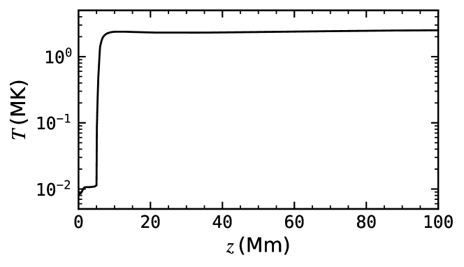
   Figure 1: The vertical distribution of the temperature before the filament is introduced.

2. We place a bulk of dense plasma around the magnetic dips to represent a filament thread, whose density profile takes the following form:

   $$\rho=\rho_{co}+\delta{\rho}\,e^{-\frac{(x-x_{0})^{4}}{w_{x}^{4}}-\frac{(z-z_{0})^{4}}{w_{z}^{4}}},$$ (7)

   where $(x_{0},z_{0})=(0,19.8)\,\mathrm{Mm}$ is the position of the mass center, $w_{x}=4\,\mathrm{Mm}$, $w_{z}=3\,\mathrm{Mm}$; $\rho_{co}$ is the plasma density in the ambient corona obtained from Step (1) and $\delta{\rho}=99\,\rho_{co}$. The corresponding temperature, $T$, is also modified so that $\rho T$ remains unchanged. We then perform MHD simulations again.

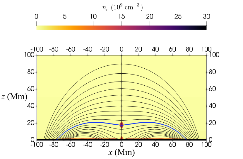
Figure 2: The distributions of the magnetic field (black lines) and the plasma density (color scale) used as the initial conditions for this paper. The blue line marks the single magnetic field line threading the centroid of the filament.

It is seen that the whole system evolves gradually. While plasmas is sucked into the filament thread due to thermal instability, the filament oscillates with an initial amplitude of 16 $\rm{km~{}s}^{-1}$. After $\sim$290 minutes, the amplitude of the filament transverse oscillation is still around 0.2 km s^-1. In order to speed up the decay, we set the velocity to be 0 everywhere in the simulation domain when the filament is at its equilibrium position. As a test, we continue the simulation and find the residual maximum velocity is only 0.06 km s^-1. Now, the system approaches a new equilibrium state, where the filament becomes $\sim$5.5$\,\mathrm{Mm}$ long in the $x$-direction and $\sim$10$\,\mathrm{Mm}$ thick in the $z$-direction. The center of mass drops to $z_{c}=17.7\,\mathrm{Mm}$. The distributions of the magnetic field and plasma density are displayed in Figure 2 as solid lines and color scales, respectively. Such a state is taken to be the real initial conditions for the simulation work to be presented in this paper. Note that there is a second plasma condensation near the original point as shown in Figure 2, which is formed due to thermal instability, and is not relevant to the study in this paper.

According to Zhang et al. (2013), the oscillation properties do not depend on the type of perturbations, no matter it is due to impulsive momentum or localized heating. In this work we choose the former one. Similar to Luna et al. (2016), the filament is perturbed with a magnetic field-aligned velocity, which is expressed as

$$\boldsymbol{v}_{0}=v_{0}\boldsymbol{b}\,e^{-\frac{(x-x_{0})^{4}}{\tilde{w}_{x}}-\frac{(z-z_{0})^{4}}{\tilde{w}_{z}}},$$ (8)

where $v_{0}=20$ $\rm{km~{}s}^{-1}$and $\boldsymbol{b}$ is the same as in Equation (5), while $\tilde{w}_{x}=15\,\mathrm{Mm}$ and $\tilde{w}_{z}=10\,\mathrm{Mm}$. The ensuing evolution is calculated with the MPI-ARMVAC code. It is noted here that we also simulate adiabatic cases for comparison, where the radiation and heat conduction in Equation (3) are removed.

3 Results

3.1 2D non-adiabatic case

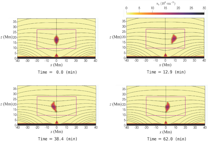
Figure 3: Evolution of the magnetic field (solid lines) and the plasma density (color scale). For comparison, the initial magnetic field is overplotted as the dashed lines.

In this subsection, we present the numerical results in the 2D non-adiabatic case. The evolution of the filament oscillation is depicted in Figure 3, where the color represents the density and the solid lines correspond to the evolving magnetic field. To illustrate how the magnetic field is deformed, the initial magnetic field is overplotted as the dotted lines. It is seen that, after the velocity perturbation is imposed on the filament, the filament begins to oscillate, but the amplitude decays rapidly. It is also noticed that the upper and lower parts of the filament do not oscillate in phase since they have different oscillation periods, which are determined by different curvature radii of the local magnetic field (see also Luna et al., 2016). As a result, the filament changes its shape continuously.

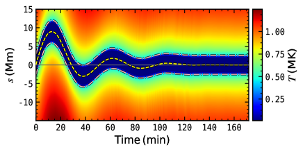
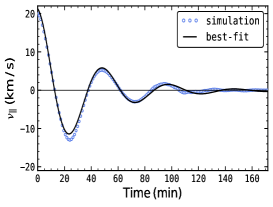
Figure 4: Left: Time-distance diagram of of the temperature distribution along the magnetic field line threading the filament centroid. Right: Evolution of the field-aligned velocity of the filament centroid.

In order to analyze the oscillation behavior more quantitatively, we extract the magnetic field line that passes through the initial centroid of the filament, which is indicated by the blue line in Figure 2. This field line is rooted at the position with $x=\pm 76.8$ Mm and $z=0$. The time-distance diagram of the temperature distribution along this line is plotted in the left panel of Figure 4, where the origin of the distance is set at $x=0$. The filament corresponds to the blue area, whose center is indicated by the yellow dashed line, and whose boundaries are marked by the two dot-dashed lines. The filament velocity along the field line ($v_{\parallel}$) is determined by the velocity of the filament centroid, and its evolution is displayed in the right panel of Figure 4 as the blue circles. It has the typical damped sinusoidal profile. Therefore, we fit $v_{\parallel}$ with the following damped sine function via the least-square method,

$$v_{\parallel}=v_{0}e^{-t/\tau}\sin\big{(}2\pi t/P+\varphi\big{)},$$ (9)

where $v_{0}$ is the initial amplitude, $P$ is the oscillation period, $\tau$ is the decay time, and $\varphi$ is the phase angle. It turns out that $v_{0}=20$ $\rm{km~{}s}^{-1}$, $P=49$ minutes, $\tau=38$ minutes, and $\varphi=\pi/2$. The fitted curve is overplotted in the right panel of Figure 4 as the black line. It is seen that the fitting is reasonable for the first 1.5 periods, and the deviation becomes remarkable after that. It is evident that the oscillation period should be shorter and shorter, rather being a constant, in the late stage of the evolution.

3.2 1D non-adiabatic case

In order to find out what new effects are brought by the two dimensions, we perform a 1D non-adiabatic hydrodynamic simulation for comparison. In order to make the comparison meaningful, the magnetic configuration in the 1D case is taken from the initial magnetic field line across the filament centroid, i.e., the blue line in Figure 2. Similar to the initial condition-producing procedure for the 2D simulation, a segment of filament is inset into the magnetic dip, with the length and density identical to the 2D case.

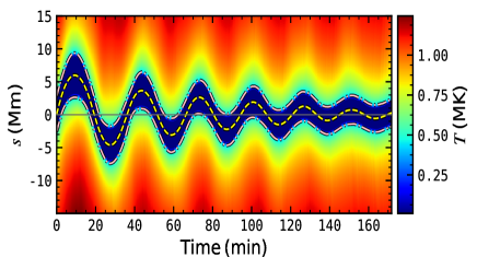
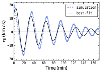
Figure 5: Left: Time-distance diagram of the temperature distribution in the 1D non-adiabatic case. Right: Evolution of the velocity of the filament centroid in the 1D non-adiabatic case.

After the same velocity perturbation is imposed on the filament, the filament thread starts to oscillate. The time-distance diagram of the temperature distribution is displayed in the left panel of Figure 5. The evolution of the velocity at the filament center is shown in the right panel as the the blue circles. Similar to the 2D case, the velocity evolution is also fitted with a damped sine function the same as Equation (9) with the least-square method. It is revealed that the oscillation period is 30 minutes and the decay time is 76 minutes. In this case, the variation of the period is more obvious since the deviation from the fitted curve with a fixed period becomes larger and larger.

3.3 1D and 2D adiabatic cases

For comparison, we also numerically simulated the adiabatic cases in both 1D and 2D. Since the evolutions are similar, the details are not described here. However, the fitting results are presented as follows: In the 1D adiabatic case, the oscillation period is $P$=37 minutes, and it is almost decayless; In the 2D adiabatic case, the oscillation period is $P$=44 minutes, and the decay time is $\tau$=211 minutes.

4 Discussions

Based on the analysis of 196 filament longitudinal oscillation events observed in 2014, Luna et al. (2018) found that the ratio of the damping time to the period $\tau/P$ can be as small as 0.6. Several factors may contribute to the damping. The primary one is the non-adiabatic processes including radiation and heat conduction, as investigated via simulations by Zhang et al. (2012). However, their results indicate that radiation and heat conduction are not enough to account for the observed damping, and other factors should play a role as well. One possible candidate is the mass change. According to Luna & Karpen (2012), the mass accretion due to continual thermal condensation would speed up the damping. This is understandable since increasing mass leads to deceasing velocity in order to conserve the total momentum. Interestingly, according to Zhang et al. (2013), mass drainage would also lead to stronger damping. They showed that when the amplitude of the filament longitudinal oscillation is too large, part of the filament material drains down across the apex of the magnetic dip. The mass drainage takes away part of the mechanical energy of the filament, leading to stronger damping as well. The second additional candidate is the thread-thread interaction. As demonstrated by Zhou et al. (2018), when there are two dips (hence two filament threads) along one magnetic field line, the two threads exchange kinetic energy, leading to weaker decay for one thread and stronger decay for the other. The third additional candidate is the deformation of the magnetic field lines, which would generate kink waves propagating outward. In this case, the oscillation energy is taken away via wave leakage. The significant feature of the filament longitudinal oscillations in our 2D non-adiabatic case is the rapid decay, where the decay time $\tau$ is only 0.7 times the oscillation period $P$, i.e., $\tau=0.7P$, in contrast to $\tau=2.5P$ in the 1D non-adiabatic case (Zhang et al., 2012). Since there are no significant mass change and thread-thread interaction here, we discuss how the non-adiabatic processes and wave leakage affect the damping.

4.1 Understanding the damping due to non-adiabatic processes

Figure 6: Snapshots of the gas pressure distribution along the magnetic field line crossing the filament centroid, where the thatched areas corresponds to the filament, and the magenta arrows indicate the velocity of the filament.

From the energy point of view, it is straightforward to understand how the filament longitudinal oscillations decay faster because of radiation and heat conduction (see Zhang et al., 2013, for details). It is simply because radiation and heat conduction take away the energy of the oscillating filament. In this subsection, we try to understand the damping process from the force point of view.

For longitudinal oscillations, Lorentz force does not play a role directly, and gravity is always a restoring force. Therefore, from the dynamics point of view, the only possible force for the decay is the gas pressure difference between the left and right boundaries of the filament. Figure 6 displays four snapshots of the gas pressure distribution along the blue line marked in Figure 2. It is seen that, different from the field-aligned gravity, the pressure gradient force is mostly opposite to the filament velocity, rather than to the filament displacement. To see this more clearly, Figure 7 displays the evolution of the filament displacement in panel (a), the evolution of the filament velocity in panel (b), and the evolution of the pressure gradient force per square centimeter ($F_{p}$) in panel (c). It is revealed that the pressure gradient force is almost antiphase with the filament velocity, with a small phase difference. Considering the slight phase shift, we decompose the pressure gradient force $F_{p}$ into two parts. The first part, $F_{p1}$, is obtained by shifting the $F_{p}$ profile so that the new profile is exactly antiphase with $v_{\parallel}$. This is done by taking the maximum running correlation coefficient between $F_{p1}$ and $v_{\parallel}$. Therefore, $F_{p1}$ can be considered as the viscous force. $F_{p2}$ is simply the residual. Panel (d) of Figure 7 displays the evolutions of $F_{p1}$ (black solid line) and $F_{p2}$ (red dashed line). It is seen that $F_{p1}$ is dominant, i.e., for the non-adiabatic case, the pressure gradient force acts mainly as a damping force, and only a minor part of it, $F_{p2}$, contributes slightly to the restoring force since it is antiphase with the filament displacement ($s$).

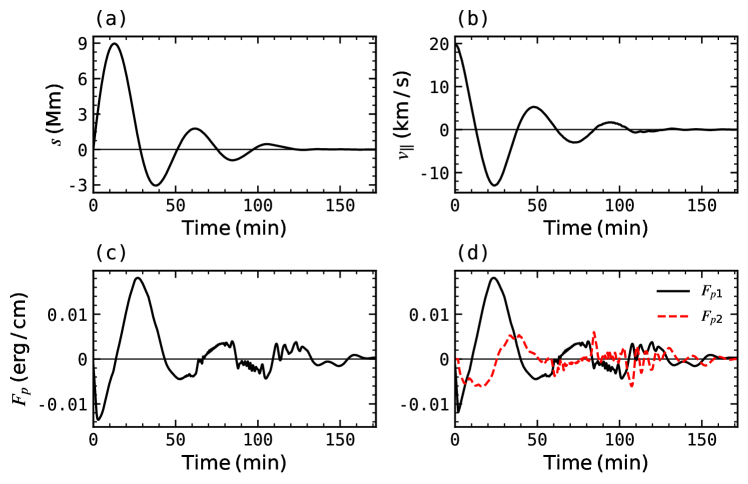
Figure 7: Evolution of several quantities in the 2D non-adiabatic case. Panel (a) is for the filament displacement along the magnetic field line, panel (b) is for the filament velocity along the magnetic field line, panel (c) is for $F_{p}$, the pressure gradient force across the left and right boundaries of the filament per square centimeter, and panel (d) is for $F_{p1}$ and $F_{p2}$, the two decomposed parts of $F_{p}$.

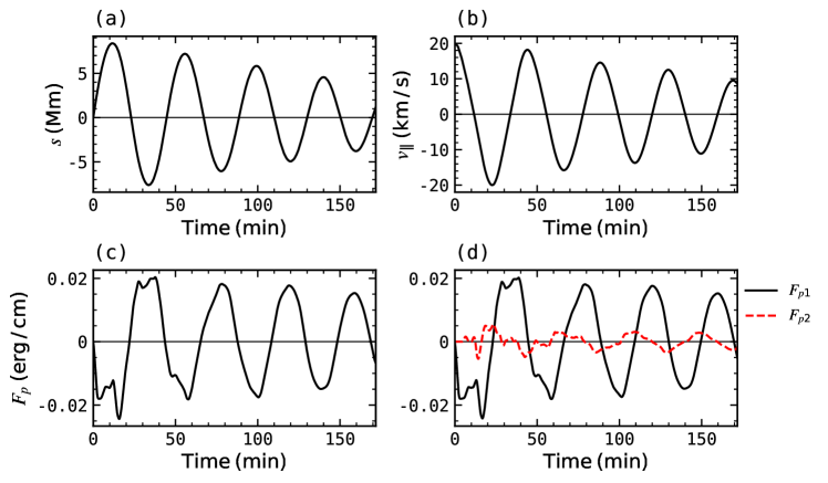
Figure 8: The same as Figure 7, but for the 2D adiabatic case.

For comparison, Figure 8 displays the evolutions of the filament displacement (panel a), field-aligned velocity (panel b), gas pressure gradient force $F_{p}$ (panel c), and the decomposed two forces (panel d) in the 2D adiabatic case. It is seen that the pressure gradient force $F_{p}$ is roughly proportional to the filament displacement $s$ with a negative coefficient, rather than proportional to the filament velocity as in the non-adiabatic case. That is to say, the pressure gradient force $F_{p}$ acts mainly as a restoring force in the 2D adiabatic case, though it is weaker than the gravity. Similar to that in the previous paragraph, we decompose $F_{p}$ into two components, $F_{p1}$ (black solid line) and $F_{p2}$ (red dashed line), where $F_{p1}$ is obtained by shifting $T_{p}$ to be exactly antiphase with $s$, and $F_{p2}$ is the residual, i.e., $F_{p2}=F_{p}-F_{p1}$. It is seen that in the non-adiabatic case, the dominant component of the pressure gradient, $F_{p1}$, contributes to the restoring force (see Luna et al., 2016, as well), and only the minor component, $F_{p2}$, contributes to the damping. This explains why the damping time is much longer in the 2D adiabatic case.

From the above analysis, it is revealed that in the adiabatic case, the gas pressure gradient force mainly acts as a restoring force, i.e., when the filament is to the right away from the equilibrium position, the coronal plasma on the right part is compressed with a higher gas pressure. However, when radiation and heat conduction are included, it is always the upstream side of the filament that has higher gas pressure, making the pressure gradient force almost a viscous force. In order to understand the reason for the difference, we examine the evolution of the thermal parameters in the two coronal segments on the two sides of the filament along the magnetic flux tube. It is found that, as the filament moves to the right, the right-hand coronal segment is compressed (and the left-hand coronal segment is rarefied), leading to higher gas pressure and density on the right (and lower pressure and density on the left). As a result of the higher density, the radiative cooling is enhanced on the right side (and weakened on the left). As time goes on, the temperature decreases on the right side (and increases on the left side), leading to lower gas pressure on the right side soon after the filament reaches its rightmost position (and higher gas pressure on the left side). Consequently, the pressure gradient force mainly acts as a viscous force. Note that radiation and heat conduction are important since the timescales of radiation and heat conduction in the corona, tens of minutes, are comparable to the period of the filament longitudinal oscillations. It is expected that they are much less important for filament transverse oscillations since the period of the latter is several times shorter.

4.2 Damping due to wave leakage

Comparing the 2D non-adiabatic and 1D non-adiabatic cases, it is revealed that the decay time in the 2D case is only half that in the 1D case. It is seen that the 2D filament longitudinal oscillations decay faster than the 1D oscillations. Such a difference is also seen between the 2D adiabatic and 1D adiabatic cases, where the latter is decayless and the former has a decay time of 76 minutes. We conjecture that the additional energy loss mechanism of the 2D effect is wave leakage. The reason is that the plasma $\delta$ in our paper, i.e., the ratio of gravity to Lorentz force, is close to unity, so the longitudinal oscillations of the filament would deform the magnetic field, and the deforming magnetic field would generate transverse waves, which then propagate away from the filament.

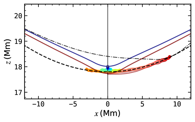
Figure 9: The trajectory of the filament centroid (colored circles) and the magnetic field lines across the filament centroid, where the red line corresponds to the initial state, the dash-dotted line corresponds to the moment when the filament reaches its rightmost position, and the blue line corresponds to $t=171.75$ minutes. The dashed line is a fitted circular arc with a radius of 70 Mm. Note that the horizontal and vertical axes are not to scale.

In order to confirm it, we plot the evolution of the magnetic field line threading the filament centroid at the initial (red line) and the final (blue line) times in Figure 9. In this figure, the trajectory of the filament centroid is overplotted as small colored circles, where the color coding from red to blue indicates the time elapse. We can see that, as the filament moves, the magnetic field line is deformed by at least $\sim$0.5 Mm.

Figure 10: Evolution of the vertical velocity of the filament, showing a decayed transverse oscillation.

As expected, such deformation would excite filament transverse oscillations. Figure 10 displays the temporal evolution of the vertical velocity of the filament centroid in the 2D non-adiabatic case. It is seen that short-period oscillations are superposed on a quickly damped oscillations with a larger period. The short-period oscillation has a period of 6.38 minutes, which is in the typical range of filament transverse oscillations (Tripathi et al., 2009; Hillier et al., 2013), whereas the quickly-damped oscillation has a period of 25 minutes, which is about half of the filament longitudinal oscillation. The half period is expected when a filament is oscillating along a dipped magnetic field. Note that the amplitude of transverse oscillation induced by the longitudinal oscillation is only 0.2 $\rm{km~{}s}^{-1}$, which is in the lower range detected by the Hinode satellite (Hillier et al., 2013), and much smaller than the velocity amplitude of filament transverse oscillations indcued by coronal waves, e.g., 8.8 $\rm{km~{}s}^{-1}$ in Liu et al. (2012) and 65–89 $\rm{km~{}s}^{-1}$ in Shen et al. (2014).

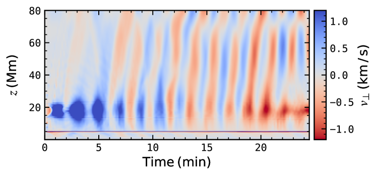
Figure 11: Time-distance diagram of the vertical velocity ($v_{\perp}$) along the $z$-axis at $x=0$.

As the magnetic field line across the filament oscillates vertically, it is anticipated to see fast-mode waves being excited. To demonstrate the fast-mode wave generation, we plot the time evolution of the $v_{z}$ distribution along the $z$-axis in Figure 11, where blue color means upward velocity and red color means downward velocity. It is seen that quasi-periodic waves propagate both in the upward and the downward directions. The period of the wave train is calculated to be $\sim$6.38 minutes based on wavelet analysis, which is almost identical to that of the filament transverse oscillation. The propagation speed of the fast-mode waves as indicated by the slope of the oblique ridges is measured to be $810\pm 60$ km s^-1, the typical fast-mode wave speed in the background corona.

In order to quantify how much energy is taken away by the fast-mode MHD waves, we select a fixed rectangular region around the oscillating filament as indicated by the pink box in Figure 3. Note that the box is large enough so that the filament is always inside the box. Within the box, we calculate the kinetic energy convected into the box ($E_{e_{\mathrm{k}}}=-\oint_{L}e_{\mathrm{k}}\boldsymbol{v}\cdot\boldsymbol{n}dl$, where $e_{\mathrm{k}}$ is the kinetic energy density, $\boldsymbol{n}$ is the normal vector, and $l$ is the length along the box boundary), the work done by Lorentz force ($E_{B}=\iint_{\Sigma}\boldsymbol{v}\cdot(\boldsymbol{j}\times\boldsymbol{B})d\sigma$, where the integral is done over the whole area of the box), and the work done by gas pressure ($E_{p}=-\iint_{\Sigma}\boldsymbol{v}\cdot\nabla pd\sigma$, where the integral is done over the whole area of the box). We also calculate the work done by gravity inside the box ($E_{g}=\iint_{\Sigma}\boldsymbol{v}\cdot\boldsymbol{F}_{g}d\sigma$, where the integral is done over the whole area of the box). The evolution of the four parts of the accumulating energy is displayed in Figure 12, where the pink area corresponds to the influx of the kinetic energy, the yellow area corresponds to the work done by Lorentz force, the blue area represents the work done by gas pressure, the green area represents the work done by gravity, and the red line corresponds to the sum of all the terms. It is seen that near the end of the simulation when the oscillation is almost completely attenuated, the work done by Lorentz force and gas pressure is dominantly negative, meaning that most of the initial kinetic energy of the filament longitudinal oscillation is lost by the work done by Lorentz force and gas pressure. Since fast-mode magnetoacoustic waves are due to the synchronous action of the Lorentz force and the gas pressure, it further implies that the major part of the initial kinetic energy of the filament is taken away by wave leakage.

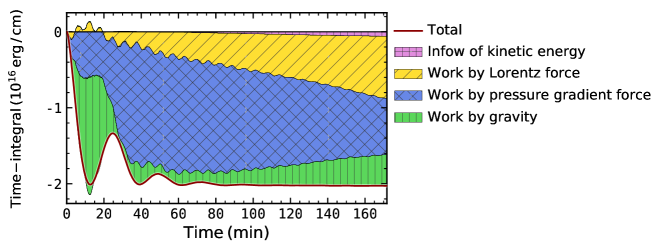
Figure 12: Time-integral of the energy loss from the fixed region indicated by the pink box in Figure 3.

Wave leakage was proposed to be able to lose the energy of an oscillating coronal loop to the surroundings (Cally, 1986). Further simulations (Brady & Arber, 2005; Selwa et al., 2006) and mode analysis (Díaz et al., 2006; Verwichte et al., 2006) indicated that in a 2D slab model, wave energy cannot be trapped, and wave leakage can efficiently attenuate the coronal loop oscillations. Terradas et al. (2006), however, pointed out that with a flux tube in a 3D magnetic configuration, wave leakage is not effective anymore, and resonant absorption becomes the dominant damping mechanism. The difference between the 2D slab model and the 3D flux tube model can be understood in an intuitional way: In the 2D slab model, whenever the coronal loop oscillates vertically, all the background magnetic field lines are pushed or pulled to oscillate. Hence, it is nor surprising that wave leakage is an efficient mechanism for the energy loss. On the other hand, in the 3D model where the flux tube is embedded in a magnetic field roughly aligned with the flux tube, when the flux tube oscillates, the ambient field lines may be pushed aside because of the third degree of freedom, and are not necessary to oscillate following the oscillating flux tube. That is to say, the oscillating slab in the 2D model is similar to a piston, which is not the case in 3D if the background magnetic field is roughly parallel to the flux tube. It is pointed out here that, however, if the background magnetic field is quasi-perpendicular to the flux tube, the oscillating flux tube would serve as a piston even in the 3D case. In this situation, all the ambient magnetic field lines would be pushed or pulled to oscillate, leading to significant wave leakage. The magnetic configuration of solar filaments is exactly like this, i.e., a sheared (and maybe twisted) core field overlain by unsheared envelope magnetic field (Chen, 2011; Parenti, 2014). As a result, when the filament, which is held by the core field, oscillates vertically, it would generate kink motions of the envelope field, leading to wave leakage.

4.3 Validity of the pendulum model

For filament longitudinal oscillations, it is often believed that the restoring force is the field-aligned component of gravity. Therefore, pendulum model was used to relate the oscillation period to the curvature radius of the dipped magnetic field, as confirmed by the 1D hydrodynamic simulations (Luna & Karpen, 2012; Zhang et al., 2012). In order to verify the pendulum model in 2D where magnetic field may react to the field-aligned motion of the filament, Luna et al. (2016) performed 2D MHD simulations, where the magnetic field around the filament is as weak as 10 G. It was found that the pendulum model still holds and there is no strong coupling between longitudinal and transverse oscillations of the filament. It is noted that, according to Zhou et al. (2018), whether the magnetic field may significantly react or not depends on the dimensionless parameter $\delta$, i.e., the gravity to Lorentz force ratio, rather than the plasma $\beta$, i.e., the gas to magnetic pressure ratio. We checked the plasma $\delta$ in Luna et al. (2016), and found that it is about 0.2, i.e., its gravity is several times smaller than the Lorentz force. Therefore, it is natural to see that the magnetic field deformation was small and the filament longitudinal oscillation did not excite significant transverse oscillation in their simulations.

In this paper, we extended the plasma $\delta$ regime to near unity. We found that fast-mode wave trains are excited and propagate upward and downward away from the oscillating filament, taking away a significant portion of the oscillation energy. With radiation and heat conduction considered, the decay time of the longitudinal oscillation is 76 minutes in the 1D simulation, and becomes 38 minutes in the 2D simulations. The deformation of the magnetic field is not trivial, which is up to 0.5 Mm as evidenced in Figure 9. Because of the deformation of the magnetic field, even the oscillation period is different between the 2D and 1D cases. As seen from Figure 9, as the filament moves to the right, the corresponding portion of the magnetic field is pressed to be flatter as indicated by the dash-dotted line in Figure 9, which results in a smaller component of the gravity along the field line. As a result, the corresponding period in the 2D case becomes longer. This explains why the oscillation period in the 1D non-adiabatic case is 30 minutes, whereas the period becomes 49 minutes in the 2D non-adiabatic case. The relative error is more than 50%. Since the curvature radius of the magnetic dip is proportional to the square of the oscillation period according to the pendulum model, the relative error of the curvature radius would be 100%. Because the gravity is comparable to the Lorentz force, the field line is strongly curved near the filament and becomes almost straight further away as evidenced by the red line in Figure 9. Such an extremely non-uniform curvature distribution accounts for the decreasing period as the oscillation attenuates seen in the right panels of Figures 4 and 5.

It is interesting to notice that, although the magnetic field line across the filament centroid is not circular, the actual trajectory of the filament is almost circular. As revealed by the colored circles in Figure 9, the trajectory fits into a circular arc (dashed line) very well.

5 Summary

In this paper, we investigated the filament longitudinal oscillations in the weak magnetic field regime. The main results are summarized as follows:

(1) Our simulations verified the suggestion proposed by Zhou et al. (2018), i.e., whether the dense plasma of a filament may modify the magnetic field is not determined by the plasma $\beta$, it is determined by the gravity to Lorentz force ratio $\delta={{\rho gL}\over{B^{2}/2\mu_{0}}}$. In our case where $\beta$ is small but $\delta$ is close to unity, the magnetic field is substantially changed by the oscillating filament. That is, low plasma $\beta$ does not guarantee that the magnetic field lines are not changed by the filament gravity. In the high $\delta$ case as in this paper, tha application of the pendulum model would lead to an error of $\sim$100% in estimating the curvature radius of the dipped magnetic field.

(2) In the framework of 2D simulations, the inclusion of heat conduction and radiation significantly reduce the decay time from 211 minutes in the adiabatic case to 34 minutes in the non-adiabatic case, implying that the non-adiabatic processes are the primary agent that dissipates the kinetic energy of the filament.

(3) With heat conduction and radiation being included, the decay time is remarkably reduced from 113 minutes in the 1D case to 34 minutes in the 2D case. It is found that the filament longitudinal oscillations excite transverse fast-mode waves, and the wave leakage is one important agent that can lose the kinetic energy of the filament.

References

- Arregui et al. (2018) Arregui, I., Oliver, R., & Ballester, J. L. 2018, Living Reviews in Solar Physics, 15, 3, doi: 10.1007/s41116-018-0012-6
- Brady & Arber (2005) Brady, C. S., & Arber, T. D. 2005, A&A, 438, 733, doi: 10.1051/0004-6361:20042527
- Cally (1986) Cally, P. S. 1986, Sol. Phys., 103, 277, doi: 10.1007/BF00147830
- Chen (2011) Chen, P. F. 2011, Living Reviews in Solar Physics, 8, 1, doi: 10.12942/lrsp-2011-1
- Chen et al. (2014) Chen, P. F., Harra, L. K., & Fang, C. 2014, ApJ, 784, 50, doi: 10.1088/0004-637X/784/1/50
- Díaz et al. (2006) Díaz, A. J., Zaqarashvili, T., & Roberts, B. 2006, A&A, 455, 709, doi: 10.1051/0004-6361:20054430
- Hillier et al. (2013) Hillier, A., Morton, R. J., & Erdélyi, R. 2013, ApJ, 779, L16, doi: 10.1088/2041-8205/779/2/L16
- Jing et al. (2003) Jing, J., Lee, J., Spirock, T. J., et al. 2003, ApJ, 584, L103, doi: 10.1086/373886
- Karpen et al. (2001) Karpen, J. T., Antiochos, S. K., Hohensee, M., Klimchuk, J. A., & MacNeice, P. J. 2001, ApJ, 553, L85, doi: 10.1086/320497
- Keppens et al. (2012) Keppens, R., Meliani, Z., van Marle, A., et al. 2012, Journal of Computational Physics, 231, 718, doi: 10.1016/j.jcp.2011.01.020
- Kippenhahn & Schlüter (1957) Kippenhahn, R., & Schlüter, A. 1957, ZAp, 43, 36
- Kuperus & Raadu (1974) Kuperus, M., & Raadu, M. A. 1974, A&A, 31, 189
- Li & Zhang (2012) Li, T., & Zhang, J. 2012, ApJ, 760, L10, doi: 10.1088/2041-8205/760/1/L10
- Lin et al. (2003) Lin, Y., Engvold, O. R., & Wiik, J. E. 2003, Sol. Phys., 216, 109, doi: 10.1023/A:1026150809598
- Liu et al. (2012) Liu, W., Ofman, L., Nitta, N. V., et al. 2012, ApJ, 753, 52, doi: 10.1088/0004-637X/753/1/52
- Luna et al. (2018) Luna, M., Karpen, J., Ballester, J. L., et al. 2018, ApJS, 236, 35, doi: 10.3847/1538-4365/aabde7
- Luna & Karpen (2012) Luna, M., & Karpen, J. T. 2012, ApJ, 750, L1, doi: 10.1088/2041-8205/750/1/L1
- Luna et al. (2016) Luna, M., Terradas, J., Khomenko, E., Collados, M., & de Vicente, A. 2016, ApJ, 817, 157, doi: 10.3847/0004-637X/817/2/157
- Parenti (2014) Parenti, S. 2014, Living Reviews in Solar Physics, 11, 1, doi: 10.12942/lrsp-2014-1
- Porth et al. (2014) Porth, O., Xia, C., Hendrix, T., Moschou, S. P., & Keppens, R. 2014, The Astrophysical Journal Supplement Series, 214, 4, doi: 10.1088/0067-0049/214/1/4
- Schure et al. (2009) Schure, K. M., Kosenko, D., Kaastra, J. S., Keppens, R., & Vink, J. 2009, A&A, 508, 751, doi: 10.1051/0004-6361/200912495
- Selwa et al. (2006) Selwa, M., Solanki, S. K., Murawski, K., Wang, T. J., & Shumlak, U. 2006, A&A, 454, 653, doi: 10.1051/0004-6361:20054286
- Shen et al. (2014) Shen, Y., Liu, Y. D., Chen, P. F., & Ichimoto, K. 2014, ApJ, 795, 130, doi: 10.1088/0004-637X/795/2/130
- Terradas et al. (2006) Terradas, J., Oliver, R., & Ballester, J. L. 2006, ApJ, 650, L91, doi: 10.1086/508569
- Tripathi et al. (2009) Tripathi, D., Isobe, H., & Jain, R. 2009, Space Sci. Rev., 149, 283, doi: 10.1007/s11214-009-9583-9
- Verwichte et al. (2006) Verwichte, E., Foullon, C., & Nakariakov, V. M. 2006, A&A, 452, 615, doi: 10.1051/0004-6361:20054437
- Vršnak et al. (2007) Vršnak, B., Veronig, A. M., Thalmann, J. K., & Žic, T. 2007, A&A, 471, 295, doi: 10.1051/0004-6361:20077668
- Wang (1999) Wang, Y.-M. 1999, ApJ, 520, L71, doi: 10.1086/312149
- Xia et al. (2018) Xia, C., Teunissen, J., Mellah, I. E., Chané, E., & Keppens, R. 2018, The Astrophysical Journal Supplement Series, 234, 30, doi: 10.3847/1538-4365/aaa6c8
- Zhang et al. (2012) Zhang, Q. M., Chen, P. F., Xia, C., & Keppens, R. 2012, A&A, 542, A52, doi: 10.1051/0004-6361/201218786
- Zhang et al. (2013) Zhang, Q. M., Chen, P. F., Xia, C., Keppens, R., & Ji, H. S. 2013, A&A, 554, A124, doi: 10.1051/0004-6361/201220705
- Zhang et al. (2017) Zhang, Q. M., Li, D., & Ning, Z. J. 2017, ApJ, 851, 47, doi: 10.3847/1538-4357/aa9898
- Zhou et al. (2018) Zhou, Y.-H., Xia, C., Keppens, R., Fang, C., & Chen, P. F. 2018, ApJ, 856, 179, doi: 10.3847/1538-4357/aab614
- Zirker et al. (1998) Zirker, J. B., Engvold, O., & Martin, S. F. 1998, Nature, 396, 440, doi: 10.1038/24798
- Zou et al. (2017) Zou, P., Fang, C., Chen, P. F., Yang, K., & Cao, W. 2017, ApJ, 836, 122, doi: 10.3847/1538-4357/836/1/122
- Zou et al. (2016) Zou, P., Fang, C., Chen, P. F., et al. 2016, ApJ, 831, 123, doi: 10.3847/0004-637X/831/2/123