Protecting Neural Networks with Hierarchical Random Switching: Towards Better Robustness-Accuracy Trade-off for Stochastic Defenses
Abstract
Despite achieving remarkable success in various domains, recent studies have uncovered the vulnerability of deep neural networks to adversarial perturbations, creating concerns on model generalizability and new threats such as prediction-evasive misclassification or stealthy reprogramming. Among different defense proposals, stochastic network defenses such as random neuron activation pruning or random perturbation to layer inputs are shown to be promising for attack mitigation. However, one critical drawback of current defenses is that the robustness enhancement is at the cost of noticeable performance degradation on legitimate data, e.g., large drop in test accuracy. This paper is motivated by pursuing for a better trade-off between adversarial robustness and test accuracy for stochastic network defenses. We propose Defense Efficiency Score (DES), a comprehensive metric that measures the gain in unsuccessful attack attempts at the cost of drop in test accuracy of any defense. To achieve a better DES, we propose hierarchical random switching (HRS), which protects neural networks through a novel randomization scheme. A HRS-protected model contains several blocks of randomly switching channels to prevent adversaries from exploiting fixed model structures and parameters for their malicious purposes. Extensive experiments show that HRS is superior in defending against state-of-the-art white-box and adaptive adversarial misclassification attacks. We also demonstrate the effectiveness of HRS in defending adversarial reprogramming, which is the first defense against adversarial programs. Moreover, in most settings the average DES of HRS is at least 5 higher than current stochastic network defenses, validating its significantly improved robustness-accuracy trade-off.
1 Introduction
Deep neural networks (DNNs) have led to substantial improvements in the field of computer vision Lecun et al. (1998); Wang et al. (2018b), natural language processing Hu et al. (2014) and automatic decision making Mazurowski et al. (2008), and have influenced a broad range of real-world applications. Nonetheless, even under a simple norm-ball based input perturbation threat model, they are recently shown to struggle with adversarial examples such as adversarial misclassification attacks Szegedy et al. (2013); Goodfellow et al. (2015); Carlini and Wagner (2017a); Su et al. (2018); Zhao et al. (2018), or adversarial reprogramming Elsayed et al. (2018), bringing about increasing concerns on model generalizability and new security threats Zhao et al. (2019).
Among different defense proposals, stochastic network defenses are shown to be promising for mitigating adversarial effects. The key idea is to replace a deterministic model with a stochastic one, with some parameters being randomized. Popular stochastic network defenses include stochastic activation pruning (SAP) Dhillon et al. (2018), defensive dropout Wang et al. (2018a) and adding Gaussian noise Liu et al. (2017). The variation of a stochastic model leads to stochastic input gradients and therefore perplexes the adversary when crafting adversarial examples. However, one critical drawback of current defenses is the noticeable drop in model performance on legitimate data (particularly, the test accuracy), resulting in an undesirable trade-off between defense effectiveness and test accuracy.
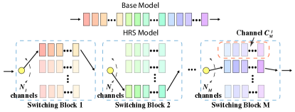
In pursuit of a better trade-off between defense effectiveness and test accuracy, in this paper we propose a novel randomization scheme called hierarchical random switching (HRS). A HRS-protected network is made of a chain of random switching blocks. Each block contains a bunch of parallel channels with different weights and a random switcher controlling which channel to be activated for taking the block’s input. In the run time, the input is propagated through only the activated channel of each block and the active channels are ever-switching. Note that each activated path in HRS-protect model features decentralized randomization for improved robustness but is also fully functional for legitimate data, which is expected to yield a better trade-off. In addition, different from the ensemble defense using multiple different networks Tramèr et al. (2017), HRS only requires one single base network architecture to launch defense.
To rigorously evaluate the adversarial robustness of the proposed HRS method, in Section 6 we adopt the security inspection principles suggested in Athalye et al. (2018) to verify the robustness claims222Appendices and codes: https://github.com/KieranXWang/HRS. Specifically, we mount four widely used adversarial misclassification attack methods (FGSM, CW, PGD and CW-PGD) under different scenarios, including standard white-box and two adaptive white-box attack settings. The adaptive attacks consider the setting where the adversary has the additional knowledge of randomization being deployed as defenses. The results show the superior defense performance of HRS, and most importantly, ensuring its robustness is indeed NOT caused by “security through obscurity” such as gradient obfuscation Athalye et al. (2018).
Below we summarize our main contributions.
-
•
We propose a novel metric called defense efficiency score (DES) that evaluates the trade-off between test accuracy and defense rate on adversarial examples, which provides a standardized approach to compare different defenses. In particular, we analyze the trade-off in state-of-the-art stochastic network defenses and adversarial training to motivate DES in Section 4.
-
•
To achieve a better robustness-accuracy trade-off, in Section 5 we propose hierarchical random switching (HRS), an easily configurable stochastic network defense method that achieves significantly higher DES than current methods. HRS is an attack-independent defense method that can be easily mounted on the typical neural network training pipelines. We also develope a novel bottom-up training algorithm with linear time complexity that can effectively train a HRS-protected network.
-
•
Compared with state-of-the-art stochastic defense methods (SAP, defensive dropout and Gaussian noise), experiments on MNIST and CIFAR-10 show that HRS exhibits much stronger resiliency to adversarial attacks and simultaneously sacrifices less test accuracy. Moreover, HRS is an effective defense against the considered powerful adaptive attacks that break other stochastic network defenses, which can be explained by its unique decentralized randomization feature (see Section 5 for details).
- •
2 Adversarial Threats
2.1 Adversarial Misclassification Attack
Fast Gradient Sign Method (FGSM) Goodfellow et al. (2015) is a \sayone-shot attack that generates an adversarial example by taking one step gradient update in the neighborhood of input image with a step size .
Carlini & Wagner (CW) attack Carlini and Wagner (2017b) formulates the search for adversarial examples by solving the following optimization problem:
| (1) |
where denotes the perturbation to . is the distortion metric; is a designed attack objective for misclassification; and the optimal term is obtained by binary search.
Projected Gradient Decent (PGD) Madry et al. (2017) is an iterative attack that applies FGSM with a small step size . It controls the distortion of adversarial examples through clipping the updated image so that the new image stays in the neighborhood of . For the -th iteration, the adversarial image generation process is:
| (2) |
where means projection to , the allowed perturbation in an ball centered at , sign applies element-wise, and is the gradient of misclassification loss.
CW-PGD Athalye et al. (2018) applies the loss term in CW attack to PGD attack. Different from CW attack, CW-PGD can directly control the level of distortion by clipping updated images into an ball of radius .
2.2 Adversarial Reprogramming
Adversarial reprogramming Elsayed et al. (2018) is a recent adversarial threat that aims at \sayreprogramming a target model trained on task into performing another task . It is accomplished by learning an input transformation and an output transformation that bridge the inputs and outputs of and . After reprogramming, the computational cost of performing task only depends on and , so that the attacker can stealthily exploit the target model.
3 Stochastic Network Defenses: Motivation and Background
Here we provide some motivation and background on why and how randomness can be exploited to defend against adversarial attacks. We are particularly interested in stochastic network defenses due to the following reasons: (i) they exhibit promising robustness performance; (ii) they are easily compatible with typical neural network training procedures; and (iii) they do not depend on specific adversarial attacks for training robust models, such as adversarial training Goodfellow et al. (2015); Madry et al. (2017).
3.1 Motivation
Why randomness can be useful in defending adversarial attacks? Here we conduct two sets of experiments and report some insightful observations. First, we find that following a randomly selected direction, the possibility of finding a successful adversarial example is very low. Second, we find that when training models with the same network architecture but with different weight initialization, each model has its own vulnerable spots. Details of these experiments can be found in Appendix11footnotemark: 1 A.
Combining these two findings, one can reach an intuitive motivation on why stochastic network defenses can be effective. As adversarial attacks are associated with worst-case performance and the model vulnerability varies with initial weight randomization, a successful attack on a stochastic model requires finding a common weakness that applies to ALL stochastic model variants. This indicates that finding an effective adversarial example for a randomized network is strictly more difficult than that for a deterministic model.
3.2 Background
There are many defense methods that utilize randomness either explicitly or implicitly. Here we summarize three representative works toward this direction.
Stochastic Activation Pruning (SAP).
Stochastic activation pruning (SAP), proposed by Dhillon et al. Dhillon et al. (2018), randomizes the neural network by stochastically dropping neuron outputs with a weighted probability. After pruning, the remaining neuron outputs are properly scaled up according to the number of pruned neurons.
Defensive Dropout.
Wang et al. Wang et al. (2018a) propose defensive dropout that applies dropout Srivastava et al. (2014) in the inference phase for defense. Defensive dropout differs from SAP in two aspects. First, it drops neurons equally regardless of their magnitudes. Second, defensive dropout is implemented in both training and testing phases, with possibly different rates.
Gaussian Noise.
Liu et al. Liu et al. (2017) introduce randomness to the network by adding Gaussian noise before each convolutional layer. Similar to defensive dropout, Gaussian noise takes place in both training and testing phases. The authors suggest to use different noise deviations for the input convolutional layer and other convolutioanl layers, which they refer to as ”init-noise” and ”inner-noise” respectively.
3.3 Stochastic Gradients
| Model | Deviation | Defense Rate (%) |
|---|---|---|
| Base | 0 | 29.18 |
| SAP | 0.0343 | 29.40 |
| Dropout 0.1 | 0.1143 | 29.60 |
| Dropout 0.3 | 0.2295 | 29.63 |
| Dropout 0.7 | 0.5186 | 32.62 |
| Gaussian | 0.6413 | 39.92 |
| HRS | 0.7376 | 61.03 |
| HRS | 0.7888 | 66.67 |
| HRS | 0.7983 | 69.70 |
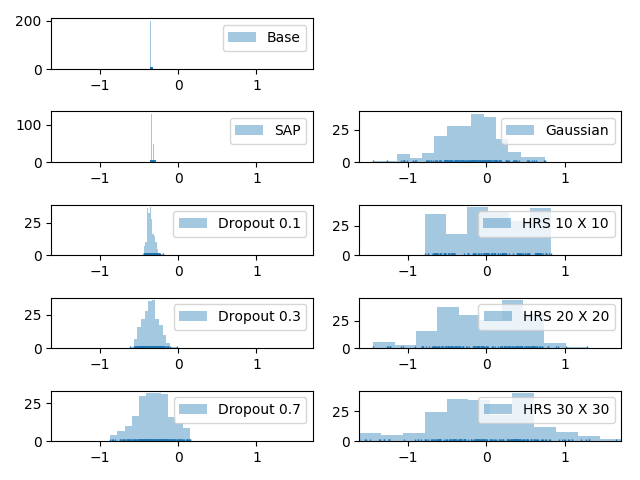
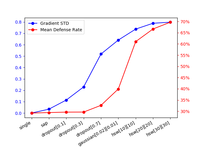
One unique property of stochastic models is the consequence of stochastic input gradients when performing backpropagation from the model output to the input. By inspecting the mean standard deviation of input gradient under different attack strengths ( constraint) over each input dimension, we find that it is strongly correlated with the defense performance, as shown in Table 1. By simply mounting a white-box attack (PGD), we find that SAP becomes as vulnerable as the base (deterministic) model, and defensive dropout and Gaussian noise have little defense effects. However, defenses that have larger standard deviations of the input gradient, such as the proposed HRS method (see Section 5 for details), are still quite resilient to this white-box attack. For visual comparison, an example of different stochastic models’ input gradient distributions under the same attack is illustrated in Figure 1.
4 Defense Efficiency Score: Quantifying Robustness-Accuracy Trade-off
For most current defense methods, there are factors controlling the defense strength. For example, in adversarial training Madry et al. (2017), one can achieve different defense strength by using different bounds on adversarial perturbations during training. Analogously, for stochastic defenses, the controlling factors are the randomization sources, such as the dropout rate, variance of Gaussian noise or the width (number of channels) in our proposed HRS approach.
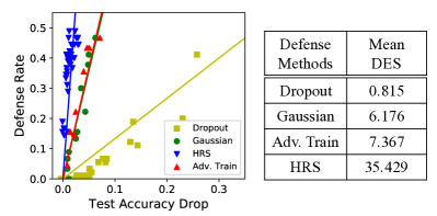
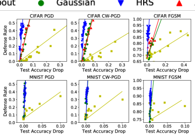
We note that although defense effectiveness can be improved by using a stronger defense controlling factor, it is traded by sacrificing the test accuracy on clean examples. We characterize this scenario in Figure 2, where the points of a certain defense method are given by using different strength factors against the same attack. For any tested defense, there is indeed a robustness-accuracy trade-off where stronger defenses are usually associated with more test accuracy drop. For example, on CIFAR-10 and under an attack strength of 8/255, when adversarial training Madry et al. (2017) achieves a 56.6% defense rate, it also causes a 7.11% drop in test accuracy, which could be an undesirable trade-off.
Therefore, it is worth noting that even under the same norm-ball bounded adversarial attack threat model, comparing different defense methods is not an easy task as they vary in both defense rate and test accuracy. In order to tackle this difficulty, we propose Defense Efficiency Score (DES) as
| (3) |
where is the gain in defense rate (percentage of adversarial examples generated by attack that fails to fool the protected model using defense scheme with strength factor ) and is the associated test accuracy drop relative to the unprotected base model333In practice, we use where is a small value (we set ) to offset noisy effect (e.g. random training initialization) leading to negative when it is close to the origin.. Intuitively, DES indicates the defense improvement per test accuracy drop.
A fair evaluation of defenses can be conducted by first choosing a desired behavior range (on either defense rate or test accuracy drop), and then compare the statistics (such as mean and variance) of DES values by varying defense strength that fall into the desired range. In Figure 2 we show the scatter plot and mean of DES values of HRS (with up to 30 X 30 channels), together with other stochastic defenses and adversarial training that have the same defense rate range. We find that the points (resulting models) of a defense lie roughly on a linear line with a small variance and our proposed HRS defense attains the best mean DES that is more than 3 higher than the state of the art, suggesting a significantly more effective defense. Details of HRS and DES analysis will be given in Section 5 and Section 6, respectively.
5 Hierarchical Random Switching (HRS)
5.1 HRS Protected Model
HRS divides a base neural network into several blocks and replaces each block with a switching block which contains a bunch of parallel channels with different weights but the same structure as shown in Figure 3. HRS features a switcher that randomly assigns the input of the block to one of the parallel channels in the run time. We call the selected channel by the switcher an active channel, and at any given time all active channels from each block constitute an active path which has the same structure as the base model.
Intuitively, a HRS-protected model can assure comparable performance to the base model if each possible path is fully functional while its random switching nature prevents the attacker from exploiting the weakness of a fixed model structure. We will introduce a training procedure to ensure full function of each path shortly.
HRS has two main advantages over current stochastic defenses. First, many defenses introduce randomness by dropping neurons or adding noise, leading to undesirable and even disruptive noisy information for model inference, deteriorating accuracy on legitimate data. This explains why these methods have worse trade-offs in terms of DES, as shown in Figure 2. In contrast, HRS introduces randomness in block switching, where each active path in HRS is trained to have a comparable performance to the base model, which greatly alleviates the issue of significant drop in test accuracy.
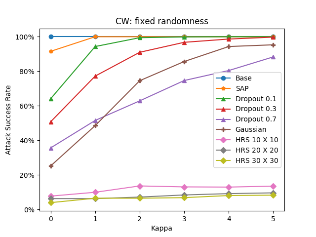
Second, HRS is a decentralized randomization scheme. Each variant of HRS has no privilege over others due to random switching. Therefore, it is fundamentally different from Dropout or Gaussian noise where all variations are derived from the base deterministic model, making the base model a centralized surrogate model and potentially leveraged by attackers to bypass these defenses. We consider this attack setting as the ”fixed-randomness” setting, which is an adaptive white-box attack assuming the attacker knows the base model and is aware of randomness being deployed as defenses. In Section 6, we will show our proposed HRS is resilient to such adaptive attack, attaining even better defense performance than standard white-box attacks.
5.2 Training for HRS
To facilitate HRS model training and ensure the performance of every path, we propose a bottom-up training approach. The training process start with training for the first switching block by constructing randomly initialized paths. These paths are trained independently to convergence, and after this round of training the weights in the first switching block will be fixed. We then train for the second switching block by constructing paths with randomly initialization except for the first switching block. During training, the switching scheme of the first block is activated, which forces the following upper blocks to adapt the variation of the first block. The training process continues until all switching blocks are trained. We find that by doing so, the training performance is stable, and each channel in a switching block is decentralized. Details of the bottom-up training approach are summarized in Algorithm 1 of Appendix B.
6 Performance Evaluation and Analysis
In this section, we run experiments on two datasets, MNIST LeCun (1998) and CIFAR-10 Krizhevsky and Hinton (2009), to benchmark our proposed HRS on defending adversarial attacks. The study consists of two parts. In the first part, We test HRS with different channels and three other stochastic network defenses in white-box attack setting (i.e. assume the attacker has full information about the target model including its structure and parameters) and two adaptive attack settings where the attackers attempt to incorporate randomness-aware counter-measures to strengthen their attacks at possibly additional computation cost. Note that for a fair comparison, we need to consider both defense effectiveness and test accuracy. Thus we set defenses to the same accuracy level by tuning their strength controlling factors and report detailed accuracy values in C.6 of Appendix C.
In the second part we provide a comprehensive study on the trade-off between defense performance and drop in test accuracy of each method via the DES introduced in Section 4. We not only compare among different stochastic defense methods but also implememt adversarial training Madry et al. (2017), a state-of-the-art deterministic defense method444We only compare adversarial training on CIFAR-10, as on MNIST it does not suffer from large test accuracy drop..
6.1 Experiment Settings
6.1.1 Base Network Models
For a fair comparison all defenses have to be applied on the same unprotected model (base model). We use two convolutional neural network (CNN) architectures as our base models for MNIST and CIFAR-10 datasets, respectively, as they were standard settings considered in previous works such as Carlini and Wagner (2017b); Papernot et al. (2016); Chen et al. (2017). Details about these base models are summarized in Appendix C.4.
6.1.2 Stochastic Network Defense Schemes
Below summarizes the implemented defenses, and Table A2 in Appendix D shows their resulting test accuracy.
-
•
SAP Dhillon et al. (2018) : Stochastic activation pruning (SAP) scheme is implemented on the base model between the first and second fully-connected layers.
-
•
Defensive Dropout Wang et al. (2018a): dropout is used between the first and second fully-connected layers with three different dropout rates, , and ( is omitted on MNIST as it severely degrades test accuracy).
- •
-
•
HRS (proposed): We divide the base model structure into two switching blocks between the first and second fully-connected layers. We implement this 2-block HRS-protected model with , and channels. Note that at any given time, the active path of HRS has the same structure as the base model.
6.1.3 Attack Settings
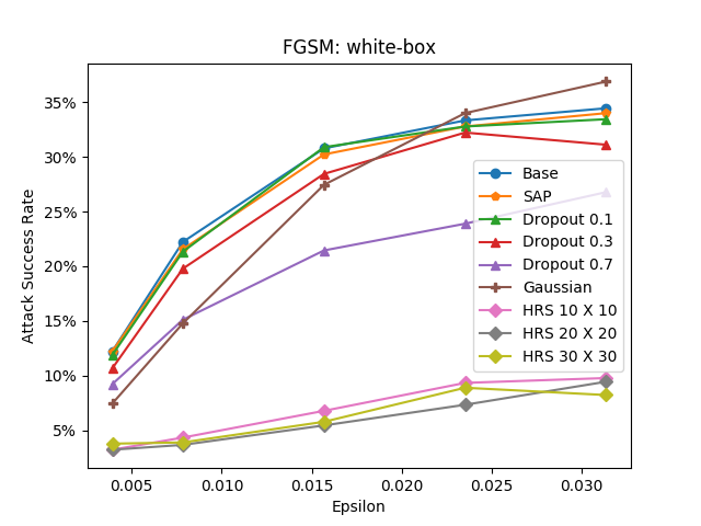
We consider the standard white-box attack setting and two adaptive white-box attacks settings (expectation over transformation (EOT)Athalye et al. (2017, 2018) and fixed randomness) for stochastic defenses. The purpose of using EOT and fixed randomness attacks is to show the defense effectiveness is not a consequence of obfuscated gradients. In each setting, four adversarial attack methods are implemented: FGSM, CW, PGD and CW-PGD. Their implementation details are summarized in Appendix C.1.
-
•
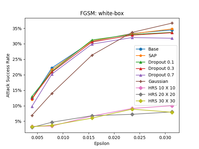
White-box Attack: The adversary uses the stochastic model directly to generate adversarial examples.
-
•
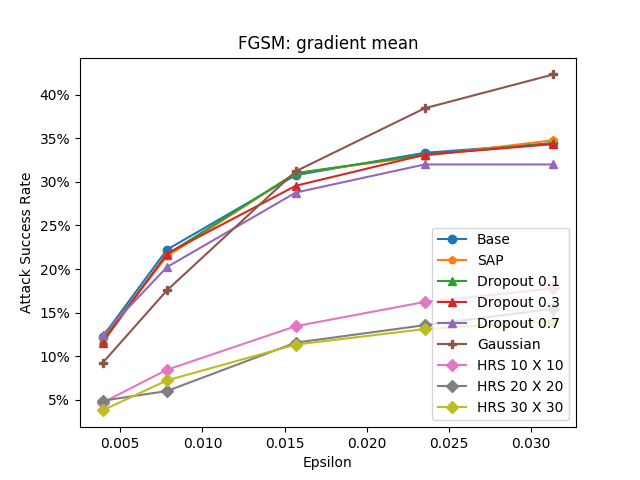
Expectation Over Transformation (EOT): When computing input gradient, the adversary samples input gradient for times and use the mean of gradients to update the perturbed example. We set in our experiments as we observe no significant gain when using . Details about the pilot research on are given in Appendix C.5.
-
•
Fixed Randomness: Generating adversarial examples using a fixed model by disabling any randomness scheme. For SAP, defensive dropout and Gaussian noise, it is done by removing their randomness generation modules (e.g. dropout layers). For HRS, it is done by fixing an active path.
6.2 White-box and Adaptive Attack Analysis
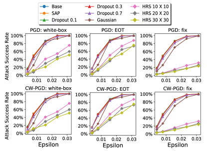
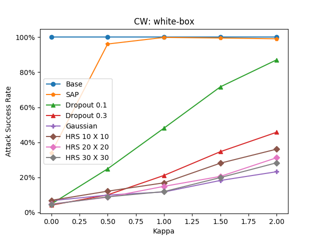
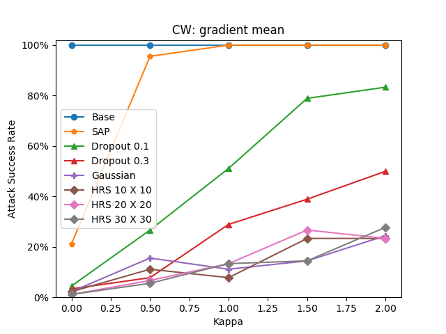
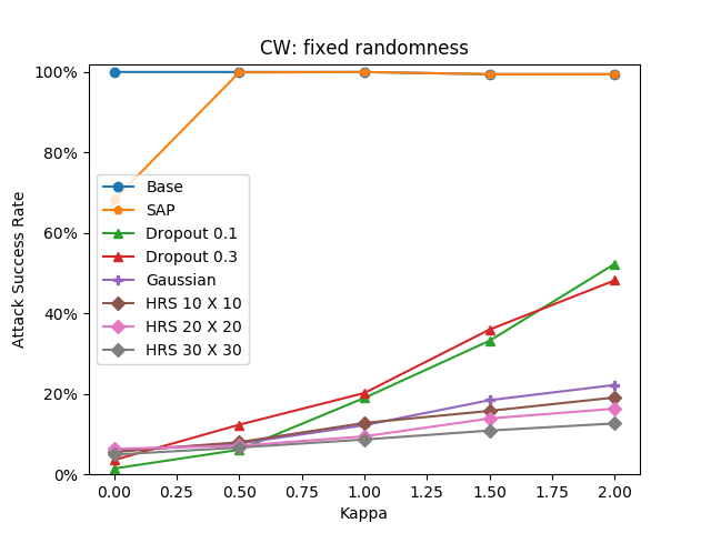
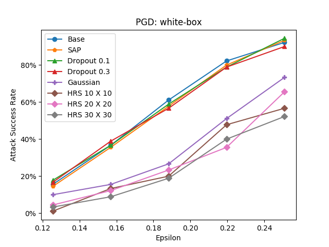
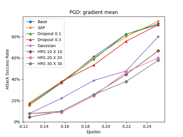
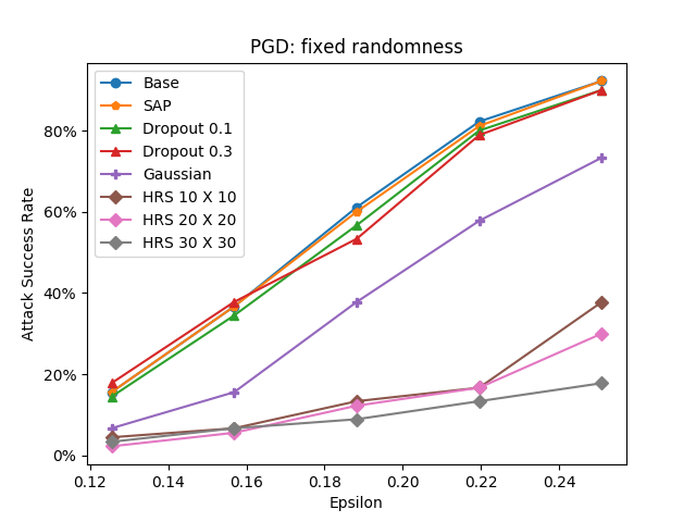
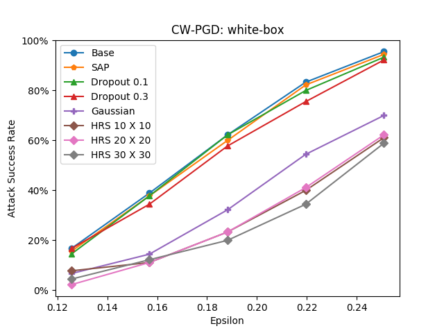
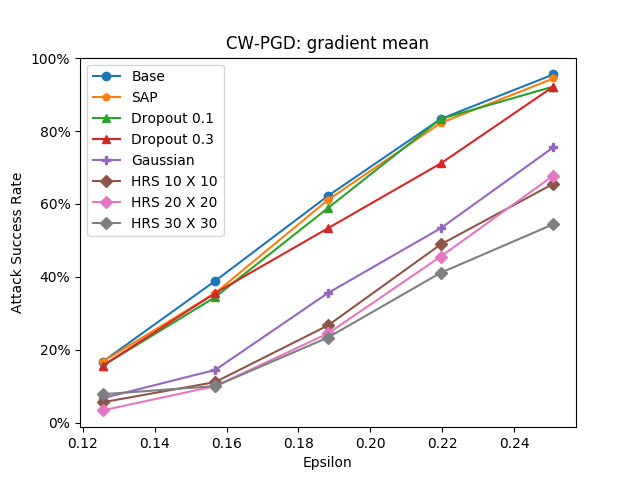
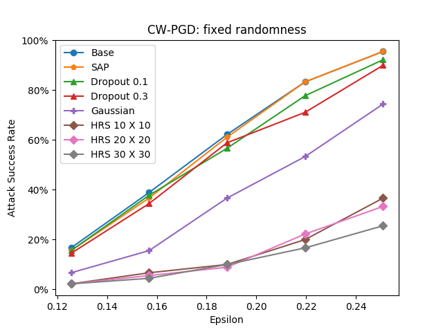
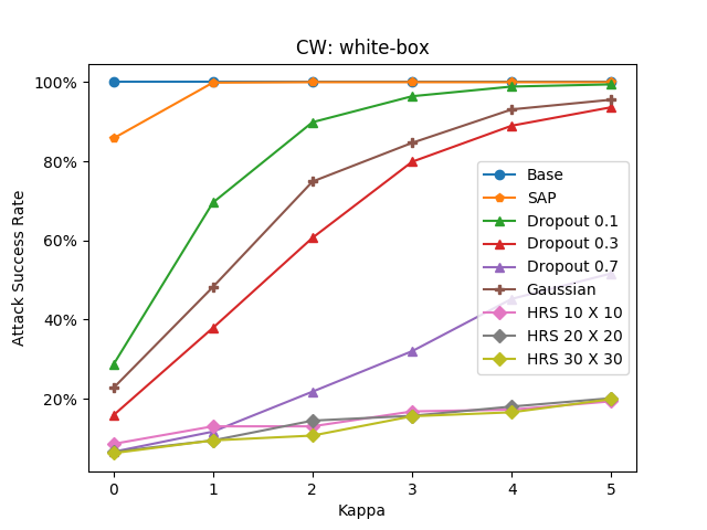
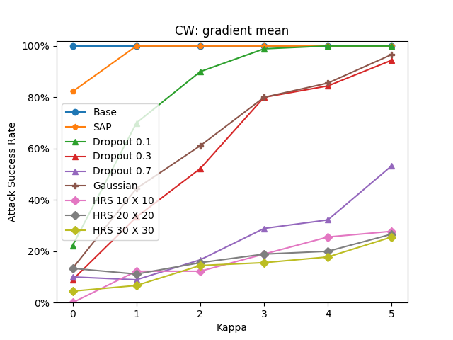
Due to space limitation, we compare the attack success rate (ASR) of different defenses on CIFAR-10 dataset against PGD and CW-PGD attacks with different strengths (the constraint) and under three attack settings in Figure 4. We defer the experimental results of FGSM and CW and all attacks on MNIST dataset to Appendix C.1.
We summarize our findings from experiments as follows:
-
1.
HRS achieves superior defense performance under all attack settings. The advantage of HRS over other defenses becomes more apparent under stronger attacks such as PGD and CW-PGD, where SAP, defensive dropout and Gaussian noise provide little defense given the same level of test accuracy drop. For example, even with a reasonably large perturbation constraint , on CIFAR-10 PGD and CW-PGD attacks only attain 51.1% and 54.5% ASRs on HRS with only at most 0.48% drop in test accuracy, respectively, while all other stochastic defenses are completely broken (100% ASR), and adversarial training with the same defense rate has 7% more test accuracy drop.
-
2.
The adaptive attacks using EOT can marginally improve ASR on all defenses when compared with the standard white-box attacks. But it is not as efficient as fixed-randomness attack or white-box attack as it requires times gradient computations.
-
3.
We observe that the fixed randomness adaptive attack leads to distinct consequences to different defense methods. For SAP, dropout and Gaussian noise, it has a similar effect as using EOT but without requiring multiple input gradient samples. However, for HRS it actually has a worse performance than standard white-box attacks. This phenomenon can be explained by the decentralized randomness property of HRS as discussed in Section 5.
-
4.
We observe that HRS with more channels are stronger in defense. Note that HRS introduces little computation overhead than the base model and it has large DEI score. In practice, further reduction of ASR with HRS can be achieved by simply allowing more channels or blocks.
6.3 Defense Efficiency Analysis
To characterize the robustness-accuracy trade-offs of different defenses, we compare the DES (see Section 4) of different stochastic defense methods in Table 2. Our HRS attains the highest DES on CIFAR-10 for all attacks and on MNIST for most attacks. In particular, HRS outperforms other defenses by a large margin (at least by ) on CIFAR-10.
| Dataset | Defense | FGSM | PGD | CW-PGD |
|---|---|---|---|---|
| MNIST | Dropout | 11.99 | 17.94 | 19.55 |
| Gaussian | 14.90 | 71.78 | 82.76 | |
| HRS | 36.41 | 76.64 | 74.90 | |
| CIFAR-10 | Dropout | 1.09 | 0.81 | 0.76 |
| Gaussian | 2.73 | 6.17 | 5.47 | |
| Adv. Train | 5.05 | 7.37 | 6.57 | |
| HRS | 32.23 | 35.43 | 35.55 |
7 First Defense against Adversarial Reprogramming
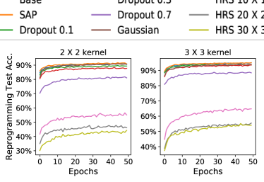
In addition to defending adversarial misclassification attacks, here we demonstrate the effectiveness of HRS against adversarial reprogramming Elsayed et al. (2018). We use the same base network on CIFAR-10 in Section 6 as the target model to be reprogrammed to classify MNIST images. We use a locally connected layer to perform the input transformation with different kernel sizes and use an identical mapping as the output transformation. The unprotected classifier can easily be reprogrammed to achieve up to 90.53% and 95.07% test accuracy using kernel sizes and , respectively, on classifying MNIST images after several epochs of training for the input transformation.
We compare the defenses against adversarial reprogramming using the same set of defense methods in Section 6 and show the reprogramming test accuracy during 50 epochs of training in Figure 6. We observe that HRS-protected models can significantly reduce the adversarial reprogramming test accuracy whereas all other defenses have less defense effect.
8 Conclusion
To fairly characterize the robustness-accuracy trade-offs of different defenses, in this paper we propose a novel and comprehensive metric called defense efficiency score (DES). In addition, towards achieving a better trade-off, we propose hierarchical random switching (HRS) for defense, which can be easily compatible with typical network training procedures. Experimental results show that HRS has superior defense performance against standard and adaptive adversarial misclassification attacks while attaining significantly higher DES than current stochastic network defenses. HRS is also the first effective defense against adversarial reprogramming.
References
- Athalye et al. [2017] Anish Athalye, Logan Engstrom, Andrew Ilyas, and Kevin Kwok. Synthesizing robust adversarial examples. arXiv preprint arXiv:1707.07397, 2017.
- Athalye et al. [2018] Anish Athalye, Nicholas Carlini, and David Wagner. Obfuscated gradients give a false sense of security: Circumventing defenses to adversarial examples. arXiv preprint arXiv:1802.00420, 2018.
- Carlini and Wagner [2017a] Nicholas Carlini and David Wagner. Adversarial examples are not easily detected: Bypassing ten detection methods. In Proceedings of the 10th ACM Workshop on Artificial Intelligence and Security, pages 3–14. ACM, 2017.
- Carlini and Wagner [2017b] Nicholas Carlini and David Wagner. Towards evaluating the robustness of neural networks. In Security and Privacy (SP), 2017 IEEE Symposium on, pages 39–57. IEEE, 2017.
- Chen et al. [2017] Pin-Yu Chen, Yash Sharma, Huan Zhang, Jinfeng Yi, and Cho-Jui Hsieh. Ead: elastic-net attacks to deep neural networks via adversarial examples. arXiv preprint arXiv:1709.04114, 2017.
- Dhillon et al. [2018] Guneet S. Dhillon, Kamyar Azizzadenesheli, Jeremy D. Bernstein, Jean Kossaifi, Aran Khanna, Zachary C. Lipton, and Animashree Anandkumar. Stochastic activation pruning for robust adversarial defense. In International Conference on Learning Representations, 2018.
- Elsayed et al. [2018] Gamaleldin F Elsayed, Ian Goodfellow, and Jascha Sohl-Dickstein. Adversarial reprogramming of neural networks. arXiv preprint arXiv:1806.11146, 2018.
- Goodfellow et al. [2015] Ian Goodfellow, Jonathon Shlens, and Christian Szegedy. Explaining and harnessing adversarial examples. 2015 ICLR, arXiv preprint arXiv:1412.6572, 2015.
- Hu et al. [2014] Baotian Hu, Zhengdong Lu, Hang Li, and Qingcai Chen. Convolutional neural network architectures for matching natural language sentences. In Advances in neural information processing systems, pages 2042–2050, 2014.
- Krizhevsky and Hinton [2009] Alex Krizhevsky and Geoffrey Hinton. Learning multiple layers of features from tiny images. Technical report, Citeseer, 2009.
- Lecun et al. [1998] Y. Lecun, L. Bottou, Y. Bengio, and P. Haffner. Gradient-based learning applied to document recognition. Proceedings of the IEEE, 86(11):2278–2324, Nov 1998.
- LeCun [1998] Yann LeCun. The mnist database of handwritten digits. http://yann. lecun. com/exdb/mnist/, 1998.
- Liu et al. [2017] Xuanqing Liu, Minhao Cheng, Huan Zhang, and Cho-Jui Hsieh. Towards robust neural networks via random self-ensemble. arXiv preprint arXiv:1712.00673, 2017.
- Madry et al. [2017] Aleksander Madry, Aleksandar Makelov, Ludwig Schmidt, Dimitris Tsipras, and Adrian Vladu. Towards deep learning models resistant to adversarial attacks. arXiv preprint arXiv:1706.06083, 2017.
- Mazurowski et al. [2008] Maciej A Mazurowski, Piotr A Habas, Jacek M Zurada, Joseph Y Lo, Jay A Baker, and Georgia D Tourassi. Training neural network classifiers for medical decision making: The effects of imbalanced datasets on classification performance. Neural networks, 21(2-3):427–436, 2008.
- Papernot et al. [2016] Nicolas Papernot, Patrick McDaniel, Xi Wu, Somesh Jha, and Ananthram Swami. Distillation as a defense to adversarial perturbations against deep neural networks. In Security and Privacy (SP), 2016 IEEE Symposium on, pages 582–597. IEEE, 2016.
- Srivastava et al. [2014] Nitish Srivastava, Geoffrey Hinton, Alex Krizhevsky, Ilya Sutskever, and Ruslan Salakhutdinov. Dropout: a simple way to prevent neural networks from overfitting. The Journal of Machine Learning Research, 15(1):1929–1958, 2014.
- Su et al. [2018] Dong Su, Huan Zhang, Hongge Chen, Jinfeng Yi, Pin-Yu Chen, and Yupeng Gao. Is robustness the cost of accuracy?–a comprehensive study on the robustness of 18 deep image classification models. In ECCV, pages 631–648, 2018.
- Szegedy et al. [2013] Christian Szegedy, Wojciech Zaremba, Ilya Sutskever, Joan Bruna, Dumitru Erhan, Ian Goodfellow, and Rob Fergus. Intriguing properties of neural networks. arXiv preprint arXiv:1312.6199, 2013.
- Tramèr et al. [2017] Florian Tramèr, Alexey Kurakin, Nicolas Papernot, Ian Goodfellow, Dan Boneh, and Patrick McDaniel. Ensemble adversarial training: Attacks and defenses. arXiv preprint arXiv:1705.07204, 2017.
- Wang et al. [2018a] Siyue Wang, Xiao Wang, Pu Zhao, Wujie Wen, David Kaeli, Peter Chin, and Xue Lin. Defensive dropout for hardening deep neural networks under adversarial attacks. In Proceedings of the International Conference on Computer-Aided Design, page 71. ACM, 2018.
- Wang et al. [2018b] Xiao Wang, Jie Zhang, Tao Xiong, Trac Duy Tran, Sang Peter Chin, and Ralph Etienne-Cummings. Using deep learning to extract scenery information in real time spatiotemporal compressed sensing. In 2018 IEEE International Symposium on Circuits and Systems (ISCAS), pages 1–4. IEEE, 2018.
- Zhao et al. [2018] Pu Zhao, Sijia Liu, Yanzhi Wang, and Xue Lin. An admm-based universal framework for adversarial attacks on deep neural networks. In 2018 ACM Multimedia Conference on Multimedia Conference, pages 1065–1073. ACM, 2018.
- Zhao et al. [2019] Pu Zhao, Siyue Wang, Cheng Gongye, Yanzhi Wang, Yunsi Fei, and Xue Lin. Fault sneaking attack: A stealthy framework for misleading deep neural networks. In Proceedings of the 56th Annual Design Automation Conference 2019, DAC ’19, pages 165:1–165:6, New York, NY, USA, 2019. ACM.
Appendix A Motivation of Using Randomness
A.1 Motivation 1
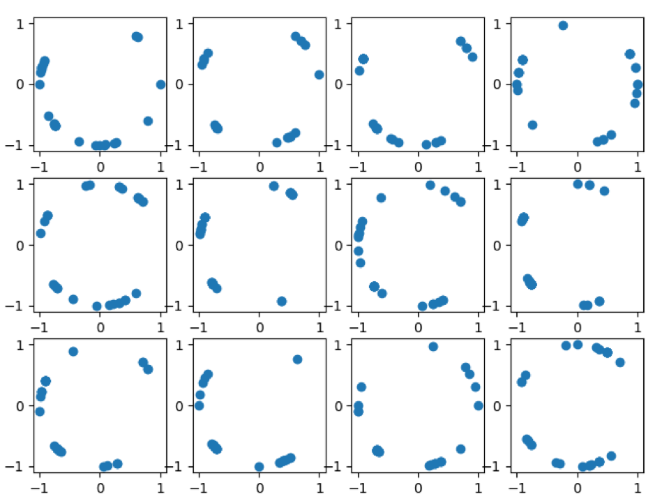
We find that when training models with the same network architecture but with different weight initialization, each model has its own vulnerable spots. Figure A1 shows the adversarial examples found by the same attack for each model. These models all have the same architecture, training process and performance in terms of test accuracy and defense capability. However, it is surprising that the distribution of adversarial examples for each model is not concentrated but quite scattered. This indicates that each model has its own robustness characteristics even though they are identical on the macro scope.
A.2 Motivation 2
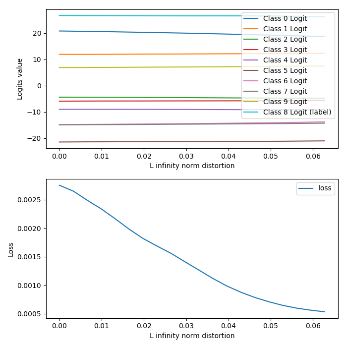
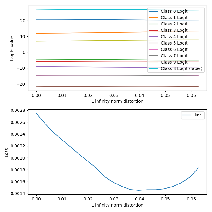
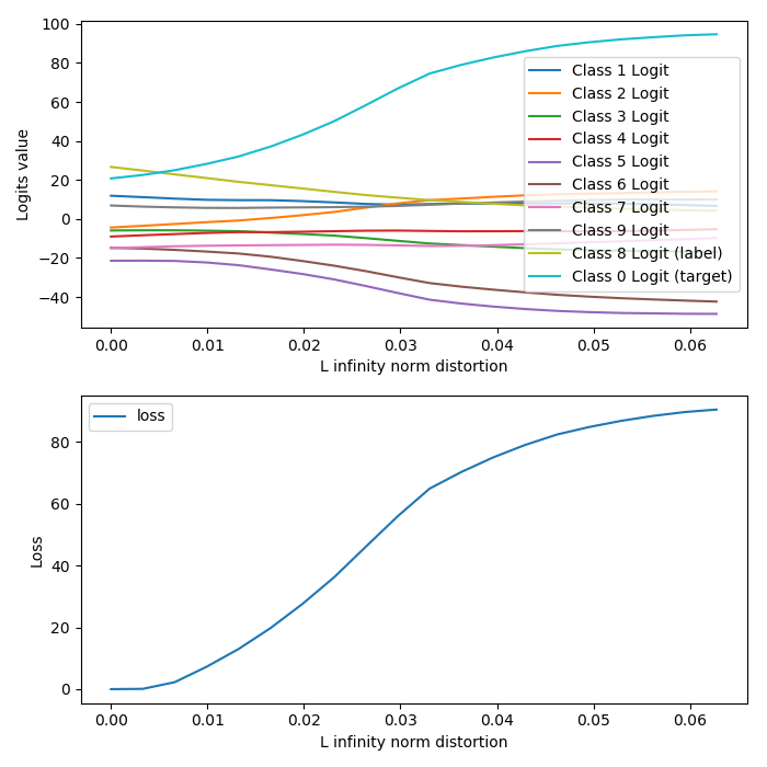
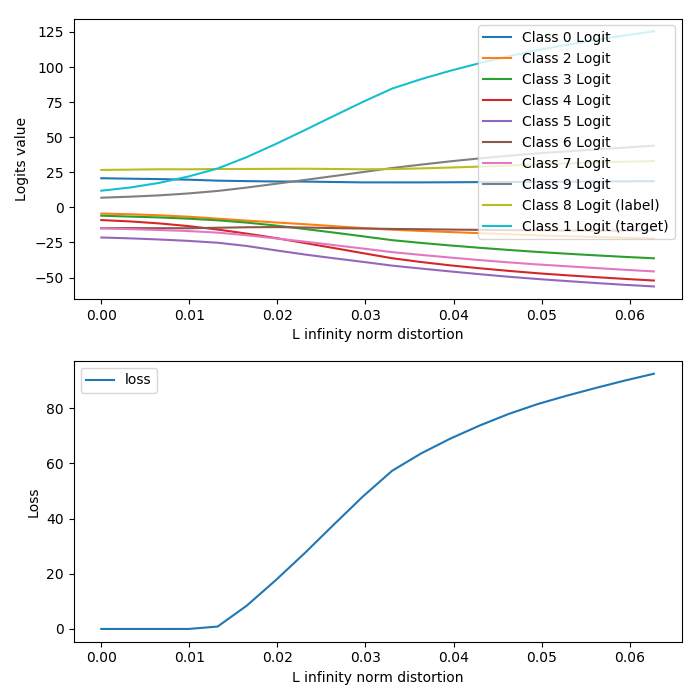
We find that following a randomly selected direction, the possibility of finding a successful adversarial example is very low. Figure A2 shows the changes of the logit (pre-softmax) layer representations and the training losses. One can observe that their changes are quite subtle and thus the model is actually quite robust to perturbations guided by random directions. In contrast, when comparing to the changes of an adversarial direction made by interpolating between a pair of original example and adversarial example found by performing targeted CW-PGD attack, the logit of the target class has a notable increase, shown in Figure A3. This indicates that although DNNs can be robustness to random perturbations, it still lacks worst-case robustness and thus becomes vulnerable to adversarial attacks.
A.3 Input Gradient Deviation v.s. Mean Defense Rate
Appendix B Training for HRS
Appendix C Experiment Details
C.1 Attack Details
All attacks are implemented in a white-box, targeted attack setting for a fair comparison. For reproducibility of the experiments, we summarize the hyper-parameters we used for each attack.
-
•
FGSM: No hyper-parameter needs to specify. Different attack strengths are given by varying the step size .
-
•
CW: We run CW attack with distortion metric. We run gradient descent for 100 iterations with step size of 0.1 and use 10 rounds binary search finding the optimal weight factor . Different attack strengths are given by varying the confidence factor .
-
•
PGD: We run gradient descent for 100 iterations with step size of 0.1. Different attack strengths are given by varying maximum allowed perturbation .
-
•
CW-PGD: The same setting as PGD.
C.2 Defense Implementation of Gaussian Noise
On MNIST, we use the recommended standard deviations which are 0.2 for the ”init-noise” (noise before the input layer) and 0.1 for the ”inner-noise” (noise before other conv layers). However, on CIFAR-10 we found this setting decreases test accuracy significantly (reducing to 60%), thus we use smaller deviations (0.02 and 0.01 respectively). We also found that using Gaussian noise solely is not sufficient to prevent the model from over-fitting. As a solution we also use dropout during training in order to prevent over-fitting.
C.3 Pilot Research on EOT
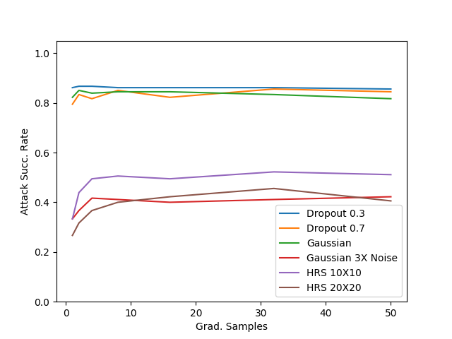
We run a pilot test to determine the value of for EOT attacks. We find using is enough as the benefits of using a larger saturates when . An example of using different values for EOT is given in Figure A5. Here we also plot Gaussian defense with a larger noise deviation which is not in Section 6.2 as it drops the test accuracy to 76.83%. The purpose is to show that the defenses that seem to be less sensitive to EOT (as shown by the lines on the top of Figure A5) do not indicate they are truly resistant to EOT.
C.4 Model Architecture
| Model for MNIST | Model for CIFAR-10 | |
|---|---|---|
| Conv layer | 32 filters with size (3,3) | 64 filters with size (3,3) |
| Conv layer | 32 filters with size (3,3) | 64 filters with size (3,3) |
| Pooling layer | pool size (2,2) | pool size (2,2) |
| Conv layer | 64 filters with size (3,3) | 128 filters with size (3,3) |
| Conv layer | 64 filters with size (3,3) | 128 filters with size (3,3) |
| Pooling layer | pool size (2,2) | pool size (2,2) |
| Fully connected | 200 units | 256 units |
| Fully connected | 200 units | 256 units |
| Output layer | 10 units | 10 units |
C.5 Implementation Details on Study of Defense Efficiency
Spots of HRS are due to different number of block channels ranging from to . Spots of dropout are due to different training and testing dropout rate ranging from 0.1 to 0.9. Spots of Gaussian noise are due to different initial and inner Gaussian noise deviations ranging from (0.01, 0.005) to (0.11, 0.055) on CIFAR-10 and from (0.1, 0.05) to (0.325, 0.1625) respectively. Spots of Adversarial Training are due to different bounds from 0.5/255 to 4.5/255 of adversarial examples used in training.
C.6 Test Accuracy
| Model | MNIST | Dev.(e-4) | CIFAR | Dev.(e-4) |
|---|---|---|---|---|
| Base | 99.04% | / | 79.17 % | / |
| SAP | 99.02% | 1.47 | 79.16 % | 2.81 |
| Dropout 0.1 | 98.98% | 3.45 | 79.08% | 7.99 |
| Dropout 0.3 | 98.68% | 6.06 | 78.65 % | 16.67 |
| Dropout 0.7 | / | / | 76.02 % | 24.52 |
| Gaussian | 99.02% | 5.82 | 78.04 % | 7.25 |
| HRS 10*10 | 98.95% | 5.33 | 78.93% | 26.81 |
| HRS 20*20 | 98.91% | 6.02 | 78.76% | 20.32 |
| HRS 30*30 | 98.85% | 8.31 | 78.69% | 23.25 |
Appendix D Experimental Results
D.1 MNIST
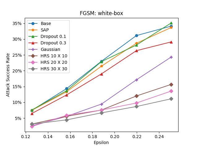
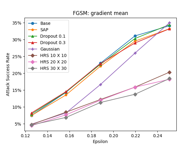
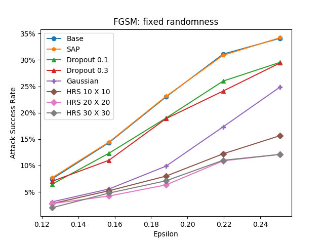
D.2 CIFAR-10
Appendix E Adversarial Reprogramming
The number of parameters in the input transformation is crucial factor to achieve high reprogramming accuracy. We applied the original input transformation in Elsayed et al. [2018] to our CIFAR to MNIST reprogramming task but find the reprogramming performance is poor due to the lack of parameters in input transformation. In order to differentiate defense effectiveness under a strong reprogramming setting, we use a local-connected layer as input transformation. The advantage of local-connected layer is that we can easily control the number of parameters by setting different kernel sizes. We found that using a kernel lead to 95.07% accuracy which is similar to reported accuracy in Elsayed et al. [2018]. We show experiment results using other kernel sizes in the following and it is clear that using a larger kernel (a large number of parameters) will lead to higher reprogramming accuracy. However, under all experiment settings we found our proposed defense demonstrate much stronger defense (lower reprogramming accuracy) compared to other defenses.
Appendix F Supplementary Experiments
F.1 The Effect of Increasing Switching Blocks
In Table A3 we compare HRS models with 1, 2 and 3 switching blocks. For all models in the comparison, there are 5 channels in each block. Thus the parameter size of these 3 models are the same. It is noted that by increasing the number of switching blocks, the resistance against adversarial attacks can be improved. So the benefit of using more switching blocks is increasing model variation given certain parameter size, and thus improving the defending effectiveness. Yet the improvement is traded with more test accuracy drop. The test accuracy of these three models are 78.78%, 78.74% and 74.92% respectively. Therefore, the number of blocks of a HRS model can be treated as a defense strength controlling factor.
| Strength | 1/255 | 2/255 | 4/255 | 6/255 | 8/255 |
|---|---|---|---|---|---|
| 1-block | 5.6% | 16.4% | 46.7% | 76.7% | 85.5% |
| 2-block | 3.3% | 10.0% | 35.6% | 64.3% | 81.2% |
| 3-block | 2.9% | 13.1% | 33.7% | 55.2% | 65.9% |