Keywords: Patlak-Keller-Segel systems, prey-taxis, indirect taxis, external signal production, stability, instability, Poincare-Andronov-Hopf bifurcation, averaging, homogenization.

Introduction

In this article, we address PDE systems formulated using the Patlak-Keller-Segel (PKS) law. Studying such systems mainly aims at modelling the pattern formation in the biological media such as the communities of living species or the biological tissues. A reader can follow the state of the research starting from review [1] to the recent review [8].

Typically, the PKS system is a reaction-advection-diffusion system into which the PKS law brings the specific nonlinear cross-diffusion. A homogeneous, or, equivalently, translationally invariant PKS system usually can stay in an equilibrium which is homogeneous too, in the sense that the density of every species is constant. Bringing the system out of such an equilibrium is necessary for occurring the non-trivial spatiotemporal patterns. An evident reason for getting out the equilibrium is the instability of it to small perturbations. In such an occasion, the non-trivial patterns can arise from the local bifurcation accompanying the occurrence of the instability. At the same time, not every spatiotemporal pattern has something to do with the local bifurcations and connecting them is sometimes unclear or not likely as in the case of soliton-like waves reported in articles [2, 3, 4]. Nevertheless, the instabilities of equilibria accompanied by the local bifurcations often are the first links in the chains of dynamical transitions leading to rather complex spatiotemporal patterns as it follows, e.g., from the observations reported in articles [5, 6, 7, 12]. The present article aims at studying the local stability issues for the counterparts of the equilibria in the systems driven by a signal produced externally. For example, such a signal can be due to fluctuating the characteristics of environment such as temperature, salinity, or the terrain relief.

Although considering the inhomogeneous PKS systems seems to be quite natural, mention- ing them in the literature is much less often than mentioning the homogeneous ones. There are several articles, e.g., [15] or [16] aimed at the topics like the global boundedness, extinction or coexistence but not at the issues we raise here. Also, we would like to mention article [14] focused on the effect of the terrain relief on the excitation of waves in a spatially distributed living community. Although this article does not consider taxis, it employs homogenization, which we use too.

It turns out that the homogenized system also takes the form of the diffusion-advection system in which the advective flux consists of two different contributions, both are emergent from the PKS cross-diffusion. The first one is the PKS cross-diffusion again, but this time it is driven by the averaged densities of the species, and the second one is the drift which is due to the external signal only. This drift is the main translator of the external signal effects. In particular, it is responsible for breaking the reflectional symmetry of the homogenized system that essentially influences the stability issues.

We examine the stability of the quasi-equilibria - that is, the simplest short-wavelength patterns fully imposed by the external signal. Comparing the results to the case of switching the signal off allows us to estimate the effect of it. We give a detailed analysis of the signals emitted as the travelling waves. The effect of such a wave on the stability of the quasi-equilibria turns out to be not single-valued but depending on the wave speed. Namely, there is an independent threshold value such that increasing the amplitude of the wave destabilizes the quasi-equilibria provided that the wave speed is above this value. Otherwise, the same action exerts the opposite effect. It is worth to note that the effect is exponential in the amplitude of the wave in both cases.

The article consists of five sections supplemented with three appendices. In section 1, we formulate the governing equations. In section 2, we address the short-wavelength external signals and describe the homogenized system. In section 3, we introduce the equilibria and quasi- equilibria. In section 4, we explore the stability and instabilities of the equilibria and quasi- equilibria. Section 5 contains the discussion on the obtained results. Appendices I, II and III contain the routine technical moments which regard the homogenization procedure, the stability analysis and asymptotics of some integral correspondingly.

1 The governing equations

For a first attempt to exploring the effect of the external signals on the stability of quasi-equilibria, we have picked out of the PKS family a system that is as simple as possible but still capable of forming the non-trivial spatiotemporal patterns due to the instabilities and local bifurcations of the homogeneous equilibria. Dimensionless form of this system reads as

$$\partial_{t}\phi=q+\kappa^{-1}f-\nu\phi+\delta_{u}\partial^{2}_{x}\phi;$$ (1.1)

$$\partial_{t}p=\partial_{x}(\delta_{p}\partial_{x}p-\kappa p\phi_{x});$$ (1.2)

$$\partial_{t}q=q(1-q-p)+\delta_{q}\partial^{2}_{x}q.$$ (1.3)

Here $x,t$ stand for a spatial coordinate and time; $\partial_{t}$ and $\partial_{x}$ denote partial differentiation with respect to coordinates $t$ and $x$; $\delta_{p},\delta_{q},\delta_{u}$, $\kappa$, $\nu$ denote the positive parameters.

Equations (1.3) and (1.2) describe the balances of densities of two interacting species. At that, equation (1.2) has got the PKS-term while equation (1.3) has not. In what follows, the species endowed (not endowed) with taxis stands as the predator (prey). We denote the predators’ and prey’ densities as $p$ and $q$, correspondingly. Note that the stimulus driving taxis is not the prey itself but another signal, intensity of which we have denoted as $\phi$. Equation (1.1) governs the production of the signal, which, in turn, gets an external contribution denoted as $f$.

It follows from equations (1.3) and (1.2) that the reproduction and losses of the prey due to predation obey the logistic and Lotka-Volterra laws correspondingly, and that the contribution from the reproduction and mortality of the predators is negligible. The last assumption makes sense if reproducing-dying the predators goes on much slower than the other processes considered.

Thus the prey-taxis modelled by system (1.1)-(1.3) is indirect in the sense that the signal is not the prey density but the intensity of some field emitted by prey. Tello & Wrozhek and also Li & Tao have addressed such kind of taxis in their recent articles [10] and [13] making focus upon the existence of the non-trivial steady states and the global boundedness of solutions. Tyutyunov et al. [11], also recently, have noticed the equivalence between the system (1.1)-(1.3) and that introduced earlier in articles [5, 6] in an attempt of taking into account the inertia of the species’ transport. The latter system reads as

$$\partial_{t}u=\partial_{x}(\kappa q+f)-\nu u+\delta_{u}\partial^{2}_{x}u;$$ (1.4)

$$\partial_{t}p=\partial_{x}(\delta_{p}\partial_{x}p-pu);$$ (1.5)

$$\partial_{t}q=q(1-q-p)+\delta_{q}\partial^{2}_{x}q.$$ (1.6)

Bringing system (1.1)-(1.3) at the inertial form (1.4)-(1.6) employs a simple ansatz $u=\kappa\partial_{x}\phi$. It introduces new dependent variable denoted as $u$ which is nothing else than the velocity of the predators advection. Equation (1.4) governs this velocity in response to the prey density and the external signal. Also, it takes into account the velocity diffusion and the resistance to the predators motion due to the environment. The coefficients of the diffusion and resistance are $\delta_{u}$ and $\nu$ correspondingly. The coefficient denoted as $\kappa$ stands as the measure of the prey-taxis intensity.

We pay attention to the formulated equivalence because the homogeneous version of the inertial system (1.4)-(1.6) (in which $f=0$) already had been studied by Govorukhin et al. and Arditi et al. in above-cited articles, and they had reported the transitions to the complex wave motions by the destabilization of the homogeneous equilibria. We’ll be considering only the inertial system (1.4)-(1.6) henceforth.

2 Homogenization and drift

In what follows, let’s consider fast variables $(\xi,\tau)$ as coordinates on 2-torus $\mathbb{T}^{2}$. Define

$$\langle g\rangle=\frac{1}{4\pi}\int\limits_{0}^{2\pi}\int\limits_{0}^{2\pi}g(x,t,\xi,\tau)\,d\xi d\tau.$$ (2.1)

Let the external signal in equation (1.4) be a short wave, i.e.

$$f=f(x,t,\xi,\tau),\ \xi=\omega x,\ \tau=\omega t,\ \omega\gg 1$$ (2.2)

and let the diffusion rates in equations (1.4-1.5) be of the same order as the wave length, namely:

$$\delta_{u}=\nu_{1}\omega^{-1},\ \delta_{p}=\nu_{2}\omega^{-1},\ \nu_{1}=\operatorname{const}>0,\ \nu_{2}=\operatorname{const}>0.$$ (2.3)

We state that under assumptions (2.2) and (2.3) the shortwave asymptotics of system (1.4)-(1.6) takes the following form

$$q(x,t)=\bar{q}(x,t)+O({\omega}^{-1}),\ \omega\to+\infty;$$ (2.4)

$$u(x,t)=\bar{u}(x,t)+\tilde{u}_{0}(x,t,\tau,\xi)+O({\omega}^{-1}),\ \omega\to+\infty;$$ (2.5)

$$p(x,t)=\bar{p}(x,t)P(x,t,\tau,\xi)+O({\omega}^{-1}),\ \omega\to+\infty;$$ (2.6)

$$\partial_{\tau}\tilde{u}_{0}=\partial_{\xi}(f+\nu_{1}\partial_{\xi}\tilde{u}_{0});\ \langle\tilde{u}_{0}\rangle=0,$$ (2.7)

$$\partial_{\tau}P=\partial_{\xi}(\nu_{2}\partial_{\xi}P-P(\bar{u}+\tilde{u}_{0})),\ \langle P\rangle=1;$$ (2.8)

$$\partial_{t}\bar{u}=\partial_{x}(\kappa\bar{q}+\bar{f})-\nu\bar{u},\ \bar{f}=\langle f\rangle;$$ (2.9)

$$\partial_{t}\bar{p}+\partial_{x}(\bar{p}(\bar{u}+\langle\tilde{u}_{0}P\rangle))=0;$$ (2.10)

$$\bar{q}_{t}=\bar{q}(1-\bar{p}-\bar{q})+\delta_{q}\partial^{2}_{x}\bar{q},$$ (2.11)

where problems (2.7)-(2.8) have to be solved on $\mathbb{T}^{2}$. Deriving this approximation (more or less routine) is placed into Appendix I.

Specifying the external signal in the form of (2.2) fully specifies equation (2.7) which determines the shortwave velocity denoted as $\tilde{u}_{0}$, which, in turn, enters the equation (2.8) as a coefficient. Then resolving the problem (2.8) and calculating the mapping $\bar{u}\mapsto\langle\tilde{u}_{0}P\rangle$ puts equation (2.10) into a form involving only unknowns $\bar{p}$ and $\bar{u}$. Hence equations (2.9), (2.10) and (2.11) form a closed system relative to unknowns $\bar{p},\bar{q}$, and $\bar{u}$ for every specific external signal. This system is called homogenized henceforth.

Equation (2.10) which is responsible for the averaged transport of the predators shows that their averaged velocity denoted as $\bar{u}$ is not the actual velocity of their advection – that is, there is some drift, the velocity of which is equal to $\langle\tilde{u}_{0}P\rangle$. The drift velocity collects the ‘shortwave remembrances’ and passes them to the homogenized system.

Let $f$ be given, we call the mapping $\mathcal{V}(f):\bar{u}\mapsto\langle\tilde{u}_{0}P\rangle$ the drift operator. We’ll be using the following notations and auxiliary notions. Let $\mathcal{G}:f\mapsto\tilde{u}_{0}$ be the transformation resulted from resolving problem (2.7). Further, let $\sigma=\operatorname{const}\in\mathbb{R}$ and smooth function $\tilde{u}_{0}=\tilde{u}_{0}(x,t,\xi,\tau)$ be given, and, moreover, let $\langle\tilde{u}_{0}\rangle=0$. We define the mapping

$$\mathcal{P}(\tilde{u}_{0}):\sigma\mapsto\langle\tilde{u}_{0}P\rangle,$$ (2.12)

where $P=P(x,t,\xi,\tau)$ is solution to problem

$$\partial_{\tau}P=\partial_{\xi}(\nu_{2}\partial_{\xi}P-P(\sigma+\tilde{u}_{0})),\quad\langle P\rangle=1.$$ (2.13)

Problem (2.13) has a unique solution for every $\sigma,\tilde{u}_{0}$ (by lemma proved in Appendix I). Once function $\tilde{u}_{0}$ is prescribed, mapping (2.12) parameterizes a path in suitable space of functions in variables $(x,t)$. Finally, we arrive at the identity

$$\left(\mathcal{V}(f)\bar{u}\right)(x,t)=\mathcal{P}(\mathcal{G}f)\bar{u}(x,t)$$ (2.14)

In fact, the short-wavelength part of the signal determines the drift in full– that is,

$$\mathcal{G}f=\mathcal{G}\tilde{f},\ \ \mathcal{P}(\mathcal{G}f)=\mathcal{P}(\mathcal{G}\tilde{f}),\ \ \mathcal{V}(f)=\mathcal{V}(\tilde{f}),\ \ \tilde{f}=f-\langle f\rangle.$$ (2.15)

Therefore, we write the drift operator as $\mathcal{V}(\tilde{f})$, $\tilde{f}=f-\langle f\rangle$, instead of $\mathcal{V}({f})$ henceforth.

Example 1

Let us consider a short travelling wave $f(x,t,\eta)=\bar{f}(x,t)+A\tilde{f}(x,t,\eta)$, where $\eta=\xi-c\tau$, $A=\operatorname{const}\geq 0$, $c=\operatorname{const}\geq 0$, and function $\tilde{f}(x,t,\cdot)$ is $2\pi$-periodic and equal to zero on average for every $(x,t)$. We’ll be using the following notation. Let $\partial_{\eta}^{-1}$ stand for the right inverse to differentiation $\partial_{\eta}$ – that is,

$$\partial_{\eta}\partial_{\eta}^{-1}w=w,\ \int\limits_{0}^{2\pi}\partial_{\eta}^{-1}w\,d\eta=0\quad\forall\ w:\ w(\cdot,\eta,\cdot)=w(\cdot,\eta+2\pi,\cdot),\ \int\limits_{0}^{2\pi}w\,d\eta=0.$$ (2.16)

. Let $g\ast h$ denote the common convolution of functions $g$ and $h$ on the real axis. Define

$$\exp_{\pm}(\sigma)=\left\{\begin{array}[]{c}\mathrm{e}^{\sigma},\ \pm\sigma>0,\\ 0,\ \mp\sigma<0,\end{array}\right.$$ (2.19)

$$s(x,t,\cdot)=-{\partial}^{-1}_{\eta}\exp_{+}^{-\frac{c}{\nu_{1}}}\ast\tilde{f}(x,t,\cdot);$$ (2.20)

where the superscript indicates raising to a power, and the convolution acts in variable $\eta$. Then

$$\tilde{u}_{0}=A\mathcal{G}\tilde{f}=\nu_{1}^{-1}A{\partial}_{\eta}s$$ (2.21)

Further, we put

$$E(x,t,\cdot)=\mathrm{e}^{as},\ a=(\nu_{1}\nu_{2})^{-1}A,$$ (2.22)

$$R(x,t,\sigma)=\left\langle\frac{E(x,t,\cdot)}{E(x,t,\cdot-\sigma)}\right\rangle,$$ (2.23)

$$z=\frac{c-\bar{u}(x,t)}{\nu_{2}}.$$ (2.24)

Let $z\neq 0$. The periodic solution to equation (2.8) has the form

$$P(x,t,z,\cdot)={\Gamma^{-1}_{\pm}}(x,t,z){E(x,t,\cdot)\left(\exp_{\pm}^{-z}\ast E^{-1}(x,t,\cdot)\right)},\quad\pm z>0;$$ (2.25)

$${\Gamma_{\pm}}(x,t,z)=\int\limits_{\mathbb{R}}\exp_{\pm}^{-z}(\sigma)R(x,t,\sigma)\,d\sigma,\ \pm z>0.$$ (2.26)

Using the Fourier series matches two expressions shown in (2.25) one to another one. Indeed, let $\hat{E}_{k}(x,t)$ and $\check{E}_{k}(x,t)$ be the Fourier coefficients of functions $E(x,t,\cdot)$ and $E^{-1}(x,t,\cdot)$ correspondingly. Then

$$P(x,t,z,\eta)={\Gamma^{-1}}(x,t,z){E(x,t,\eta)\left(\check{E}_{0}(x,t)+z\sum\limits_{k\in\mathbb{Z}\setminus\{0\}}\frac{\check{E}_{k}(x,t)\mathrm{e}^{ik\eta}}{z+ik}\right)},$$ (2.27)

$$\Gamma(x,t,z)={(\check{E}_{0}\hat{E}_{0})(x,t)+z\sum\limits_{k\in\mathbb{Z}\setminus\{0\}}\frac{(\hat{E}_{k}^{*}\check{E}_{k})(x,t)}{z+ik}}.$$ (2.28)

Given the formula (2.28), we express the drift velocity as follows

$$\mathcal{V}(A\tilde{f})\bar{u}=\langle\tilde{u}_{0}P\rangle=-\nu_{2}z\Gamma^{-1}(x,t,z){\sum\limits_{k\in\mathbb{Z}\setminus\{0\}}\frac{ik(\hat{E}_{k}^{*}\check{E}_{k})}{z+ik}}=\nu_{2}z(1-\Gamma^{-1}(x,t,z)).$$ (2.29)

(Deriving the second equality in this chain uses identity $\sum\limits_{k\in\mathbb{Z}}\hat{E}_{k}^{*}\check{E}_{k}=\langle EE^{-1}\rangle=1.$) Further, let $v$ stand for the total advective velocity involved in equation (2.10), hence,

$$v\stackrel{{\scriptstyle\mathrm{def}}}{{=}}\bar{u}+\mathcal{V}(A\tilde{f})\bar{u}.$$ (2.30)

By equality (2.29),

$$v=v(x,t,z)=c-\frac{z\nu_{2}}{\Gamma\left(x,t,z\right)}$$ (2.31)

Since

$$\Gamma(x,t,z)=\pm z\Gamma_{\pm}(x,t,z),\ \pm z>0,$$

we get additional representations for the total advective velocity, namely

$$v(x,t,z)=c\mp\frac{\nu_{2}}{\Gamma_{\pm}\left(x,t,z\right)}\ \pm z>0.$$ (2.32)

Expressions (2.26), (2.28), (2.31), (2.32) give the analytic continuation to the advective velocity to some strip parallel to the real axis in the complex plane of variable $z$. This conclusion agrees with remark 6 at the end of Appendix I.

Remark 1

Formula (2.32) (where one has to put $z=c/\nu_{2}>0$) shows that the total advective velocity is not equal to zero even if the averaged velocity denoted as $\bar{u}$ vanishes. Indeed,

$$v(x,t,c/\nu_{2})=\mathcal{V}(A\tilde{f})0=c-\frac{\nu_{2}}{\Gamma_{+}(x,t,c/\nu_{2})}\stackrel{{\scriptstyle\mathrm{def}}}{{=}}v_{e}(x,t),\ c>0.$$ (2.33)

Thus, a short travelling wave emitted as the external signal induces a residual drift determined by equality (2.33). Inspecting the case of $c=0$ with the use of formula (2.31) shows that $\mathcal{V}(A\tilde{f})0=0$ – that is, the stationary waves produce no residual drifts.

Remark 2

Let $a>0$ and $c>0$ be the characteristic amplitude and phase velocity of some signal emitted as a travelling wave. Straightforward evaluating the expression (2.33) for the values of $c$ tending to zero or infinity and for the fixed values of the other variables involved therein shows that

$$v_{e}\to 0,\ c\to+0,\quad v_{e}\to 0,\ c\to\infty.$$ (2.34)

Consider now expression (2.33) for the value of $a$ tending to zero or to infinity and for the fixed values of all other quantities. In addition, assume that $\tilde{f}(x,t,\cdot)\not\equiv 0$. Then

$$v_{e}\to 0,\ a\to+0,\quad v_{e}\to c,\ a\to\infty.$$ (2.35)

The first limit written down in (2.35) is obvious while the second is a result of estimating the integral (2.26) with the use of the Laplace method. There are more details of this issue in Appendix III.

3 Equilibria and quasi-equilibria

Henceforth, we call as quasi-equilibrium (equilibrium) a stationary solution to homogenized system (2.9-2.11) (to exact system (1.4-1.6)) such that $\bar{u}=0$ ($u=0$). Note that the definitions require uniform distributions of the species neither for the quasi-equilibria nor for the equilibria.

Given a quasi-equilibrium, formulae (2.4)-(2.6) determine the leading approximation to a special solution to the exact system displaying the short-wavelength patterns of the predators’ density and velocity. At that, the latter vanishes on average for every value of the slow variables while the former does not do so, and distributing the averaged values of it is consistent with that specified by the quasi-equilibrium.

In the considerations below, the quasi-equilibria and the related short-wavelength regimes are not distinguishable in effect. Therefore we’ll be using the same name for both.

Tuning the external signal is necessary to set an equilibrium or quasi-equilibrium. Indeed, substituting the advective velocity, $u$, with zero in the exact system simplifies it as follows

$$\delta_{q}{\partial}^{2}_{x}q+q(1-q-p)=0,\quad p=\operatorname{const}\geq 0,\quad\kappa q-\bar{f}=\operatorname{const}.$$ (3.1)

Only the nonnegative solutions to problem (3.1) make sense. However, every such solution is unbounded except for the constants. It is easy to see just looking at fig. 1. Hence $\bar{f}=\operatorname{const}$ too. Thus the translational invariance and homogeneous distributions of the species are necessary for bringing the exact system at equilibrium. In what follows, we neglect the trivial solution such that $q=0$ and arrive at homogeneous equilibria family

$$p\equiv p_{e},\quad q\equiv q_{e},\ u=0,\quad p_{e}=\operatorname{const}>0,\quad q_{e}=\operatorname{const}>0,\quad p_{e}+q_{e}=1.$$ (3.2)

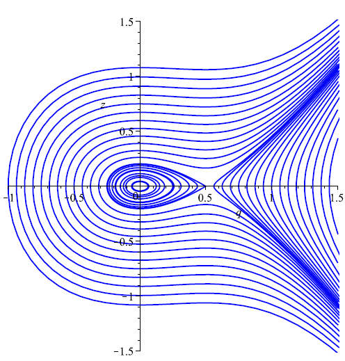
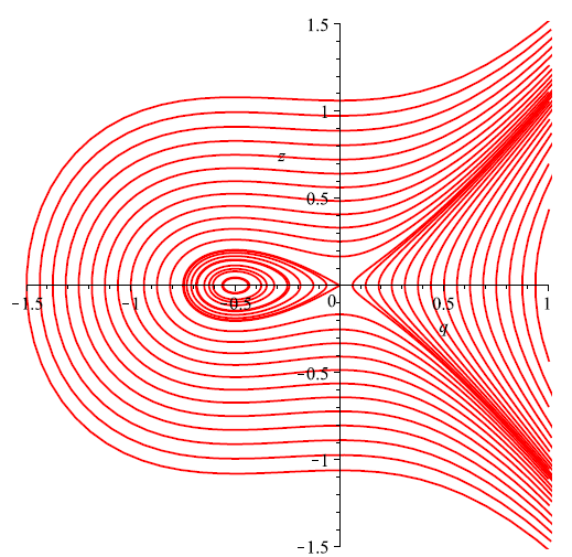
Figure 1: Phase portraits of the first equation in system (3.1). The left frame displays $p=1/2$; the right frame displays $p=3/2$.

Now let’s pass to the quasi-equilibria and consider them together with a bit more general motions of the homogenized system with zero mean velocity. The equations governing such regimes are

$${\partial}_{t}\bar{q}=\delta_{q}{\partial}^{2}_{x}\bar{q}+\bar{q}(1-\bar{q}-\bar{p}),\ {\partial}_{t}\bar{p}+{\partial}_{x}(v_{e}{\bar{p}})=0,\ v_{e}=\mathcal{V}(\tilde{f})0;\ \kappa\bar{q}-\bar{f}=\operatorname{const},\ \bar{f}=\langle f\rangle$$ (3.3)

where $v_{e}$ is the residual drift velocity. Conjecturing the existence of the suitable positive solutions to this problem links the smooth and short-wavelength parts of the signal one to another. (These are $\bar{f}$ and $\tilde{f}=f-\langle f\rangle$). Exploring these interplays is far beyond the scope of this article, but we give a couple of examples.

Example 2

Let ${f}=\bar{f}+A\tilde{f}(x,t,\xi)$ where $A=\operatorname{const}\geq 0$, and let function $\tilde{f}(x,t,\cdot)$ be $2\pi$-periodic and equal to zero on average for every $(x,t)$. Then tending $z$ and $c$ to zero in formulae (2.21) and (2.27) puts the quasi-equilibrium pattern into the following form

$$\tilde{u}_{0}=\tilde{u}_{e}=-A(\nu_{1}\partial_{\xi})^{-1}\tilde{f},\quad P=P_{e}={\langle\mathrm{e}^{as}\rangle}^{-1}\mathrm{e}^{as},\ a=(\nu_{1}\nu_{2})^{-1}A,\ {s}=-\partial_{\xi}^{-2}\tilde{f}.$$

Hence the signal does not produce the residual drift, i.e. $v_{e}=\mathcal{V}(\tilde{f})0=0$, as we have been noticing in remark 1. Hence the equation for the averaged predators’ transport reads as ${\partial}_{t}p=0$. Consequently, choosing a time-independent predators’ density, $p_{e}=p_{e}(x)$, determines the prey’s density, $q=q_{e}(x)$, that, in turn, determines signal’s average, $\bar{f}=\bar{f}_{e}$. The positiveness restriction is easy to satisfy this time. In particular, we arrive at the homogeneous family (3.2) provided that $\bar{f}_{e}=\operatorname{const}$.

Example 3

Let $f=\tilde{f}(t,\xi,\tau)$ where $\langle\tilde{f}(t,\cdot)\rangle=0$ for every $t$. Then the spatial homogeneity of the residual drift velocity is easy to see. Hence there exists the family of homogeneous quasi-equilibria (3.2). Assuming that $f=A\tilde{f}(t,\eta)$, where $\eta=\xi-c\tau$, $A=\operatorname{const}\geq 0$, $c=\operatorname{const}\geq 0$, brings us at the class of signals considered as example 1, and we get explicit expressions for the quasi-equilibrium patterns and the residual drift velocity by formulae (2.21), (2.25), and (2.33) correspondingly by substituting $z$ by $c/\nu_{2}$ in the two last ones. Note that the quasi-equilibrium patterns are the short travelling waves propagating at the same speed as those emitted externally.

4 Stabilizing and destabilizing

In what follows, we’ll be investigating an effect of the short-wavelength signals on the stability of the quasi-equilibria by comparing them to the equilibria. Such a comparison is most clear and natural in the case of homogeneous quasi-equilibria which we’ll be restricted to henceforth. Note in passing, that only an external signal vanishing on average and producing a constant in space residual drift velocity denoted as $v_{e}$, is capable of giving rise to a family of homogeneous quasi-equilibria (3.2), and vice versa. For instance, the signal satisfying both conditions can take the form $f=A\tilde{f}(x,t,\xi)$ or $f=A\tilde{f}(t,\xi,\tau)$, where $\langle\tilde{f}\rangle=0$ for every value of the slow variable as shown by examples 2 or 3.

We start with revisiting the instability of the equilibria, which is known mainly due to the prior work by Govorukhin et al. and by Arditi et al., [5],[6].

4.1 Destabilizing the equilibria

We call as homogeneous the version of system (1.4)-(1.6) arising upon switching off the external signal – that is, for $f=0$. The homogenous system is invariant to the spatiotemporal translations. There exists the homogeneous family (3.2), as we have been mentioning in the section 3.

Let’s choose out of family (3.2) an equilibrium with some specific densities $p_{e}>0$ and $q_{e}=1-p_{e}>0$. The system governing the evolution of a small perturbation of such an equilibrium reads as

$$\partial_{t}{u}+\nu{u}-{\kappa}\partial_{x}{q}=\delta_{u}\partial^{2}_{x}u,$$ (4.1)

$$\partial_{t}{p}+{p}_{e}\partial_{x}{u}=\delta_{p}\partial_{x}^{2}{p};$$ (4.2)

$$\partial_{t}{q}+q_{e}({p}+{q})=\delta_{q}\partial_{x}^{2}{q};$$ (4.3)

$${p}_{e}+{q}_{e}=1.$$

Given the invariance of system (4.1)-(4.3) to the spatiotemporal translations, we’ll be considering only the eigenmodes having the following form

$$(\hat{u},\hat{p},\hat{q})\exp(i\alpha x+\lambda t),\ \lambda=\lambda(\alpha)\in\mathbb{C},\ \alpha\in\mathbb{R}.$$ (4.4)

Here $\lambda$ is the eigenvalue of the spectral problem arising from the substituting of eigenmodes (4.4) into system (4.1)-(4.3). We say that eigenmode (4.4) is stable (unstable, neutral) if the real part of the corresponding eigenvalue is negative (positive, equal to zero). We’ll be looking for the occurrences of instability, that is, transversal intersecting the imaginary axis by a smooth branch of eigenvalues upon changing the other parameters of the spectral problem along a smooth path. If such a branch crosses the imaginary axis at a non-zero point, the instability is named as oscillatory otherwise as monotone.

It is well-known that an occurrence of instability in the family of equilibria of a smooth family of vector fields indicates the local bifurcations. If there are no additional degenerations, branching the equilibria family accompanies the monotone instability, and branching the limit cycle off the family accompanies the oscillatory instability (Poincare-Andronov-Hopf bifurcation), and more complex bifurcations happen in the case of additional degeneracy, e.g. when the neutral spectrum is multiple. For more information on this subject, a reader could refer to monographs [17, 18, 19].

It is convenient to introduce the following notation

$$\beta=\alpha^{2},\ \delta=(\nu,\delta_{q},\delta_{p},\delta_{u}).$$

Note that each equilibrium (3.2) has a neutral homogeneous mode (that corresponds to $\lambda=\alpha=0$), but this does not lead to any long-wave instabilities. To get rid of this and other unwanted degenerations, we assume the following

$$\beta>0,\ 0<p_{e}<1,\ \nu(\delta_{p}+\delta_{u}+\delta_{q})>0.$$ (4.5)

Let $\Pi$ be a domain cut out by inequalities (4.5) in the space of parameters $p_{e},\beta,\delta$. Let us consider an equilibrium of family (3.2) with specific density $p_{e}$ and its eigenmodes (4.4) with specific wavelength $\alpha=\pm\sqrt{\beta}$. There exists function

$$\kappa_{c}=\kappa_{c}(p_{e},\beta,\delta)$$

analytic in $\Pi$ and such that (i) each of those eigenmodes is stable provided that $\kappa<\kappa_{c}(p_{e},\beta,\delta)$; (ii) there is an unstable mode provided that $\kappa>\kappa_{c}(p_{e},\beta,\delta)$; (iii) there exists two conjugated neutral modes with $\lambda\neq 0$ provided that $\kappa=\kappa_{c}(p_{e},\beta,\delta)$. The oscillatory instability occurs each time a path in $\Pi\times(0,\infty)$ (where $(0,\infty)\ni\kappa$) intersects graph $\{(p_{e},\beta,\delta),\kappa_{c}(p_{e},\beta,\delta)\}$ transversally, perhaps, with except for some cases of degeneracy (Fig. 2). Note that

$$\min\limits_{0<p_{e}<1,\,\beta>0}\kappa_{c}(p_{e},\beta,\delta)=\kappa_{*}(\delta)>0$$ (4.6)

where the strict positiveness takes place for every $\delta$ obeying (4.5). For every $\kappa>\kappa_{*}(\delta)$, equation $\kappa=\kappa_{c}(p_{e},\beta,\delta)$ determines a closed curve inside semi-strip $\{0<p_{e}<1,\,\beta>0\}$. This curve widens itself and tends to the boundary of the semi-strip as $\kappa\to+\infty$.

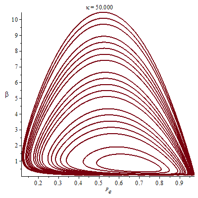
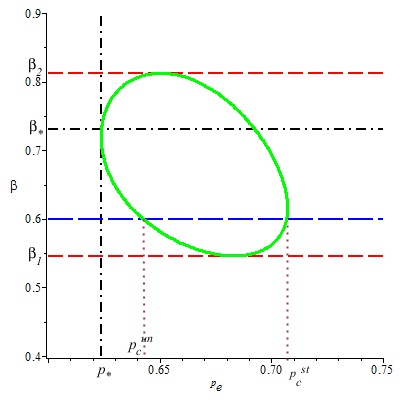
Figure 2: The left frame shows typical curves determined by equation $\kappa_{c}(p_{e},\beta,{\delta})=\kappa$ in the semi-strip $\{0<p_{e}<1,\beta>0\}$ for the values of $\kappa$ in the range from $15.12$ to $50.0$ and ${\delta}=(1,1,0,0)$. The area bounded by such a curve increases with $\kappa$ and tend to cover all the semi-strip when $\kappa\to+\infty$. At that, $\left.\kappa_{*}({\delta})\right|_{{\delta}=(1,1,0,0)}=27/2,$ and $\kappa_{c}$ takes this value at $p_{e}=2/3$, $\beta=2/3$. The right frame corresponds to ${\delta}=(1,1,0,0)$ and $\kappa=13.56$. The other numerical values are: $p_{*}\approx 0.624$; $p_{c}^{un}\approx 0.642$, $p^{st}_{c}\approx 0.707$, $\beta_{1}\approx 0.546$, $\beta_{2}\approx 0.812$.

Fig. 2 shows that the oscillatory instability of homogeneous equilibria occurs in response to increasing the specific predators’ density denoted as $p_{e}$ provided that the predators’ motility is above the threshold – that is, provided that the inequality $\kappa>\kappa_{*}(\delta)$ holds. For more details on the stability analysis, a reader can refer to the first subsection of Appendix II.

By direct numerical simulations, Govorukhin et al. and Arditi et al. demonstrated that this instability leads to exciting the waves which are time-periodical for the weakly supercritical values of $p_{e}$, and which tend to move chaotically for the greater values of $p_{e}$. Also, it turned out that the wavy motions anyway allow the predators to consume more while keeping a greater stock of prey, and, in this sense, the waves are always more advantageous than the equilibria.

At this point, it is worth to stress the role of quantity $\kappa_{*}(\delta)$ defined in (4.6). If $\kappa<\kappa_{*}(\delta)$ then neither the oscillatory instability of the homogeneous equilibrium nor the accompanying bifurcation is possible, whatever values of the predators’ density and the disturbances wavelengths are specified. In this sense, the value of $\kappa_{*}(\delta)$ is the threshold of the absolute stabilization of the homogeneous equilibria. If the predators’ motility is below this threshold for some predator-prey community, then such a community fails to adapt itself to the resource deficiency. It is important to note that $\kappa_{*}(\delta)>0$ for every $\delta$ obeying restriction (4.5).

The neutral spectrum we face upon the considered instability is always multiple. Namely, the pure imaginary pair of eigenvalues is double, and there is a simple null eigenvalue. For such a degeneration, there are two reasons. The first is the reflectional symmetry. The second is the conservation law for the predators’ density, because of which the homogeneous equilibria are not isolated but form the continuous 1-parametric family.

In the mentioned studies of the homogeneous system, Govorukhin et al. and Arditi et al. formulated the initial-boundary value problem for a bounded spatial domain with the Neumann’s boundary conditions (also known as the no-flux boundary conditions). Such setting removes the reflectional symmetry together with the multiplicity of the pure imaginary pair, but the conservation law persists. The equilibrium family and the null eigenvalue persist too. One can get rid of this residual degeneration by restricting the system on the level sets of the conserved quantity. As a result, the common theory of Poincare-Andronov-Hopf bifurcation becomes applicable to the restriction. Alternatively, one can apply the general results on the bifurcation accompanying the oscillatory instability for the vector fields, which possess the so-called cosymmetry [27].

Recently, several authors [7, 11, 12] explored the oscillatory instability and the spatiotemporal patterns it creates in more general but still homogeneous PKS systems. They considered the finite domains and employed the Neumann’s boundary conditions. Given such boundary conditions and the kinetic of species, the mentioned degenerations disappear, and the oscillatory instability follows the generic Poincare-Andronov-Hopf scenario.

4.2 Destabilizing the quasi-equilibria

Let the homogeneous quasi-equilibria form family (3.2) for some specified signal. Let’s choose out of this family a quasi-equilibrium with some specific densities $p_{e}>0$ and $q_{e}=1-p_{e}>0$. The system governing the small perturbations of such a quasi-equilibrium has the form

$$\partial_{t}\bar{u}+\nu\bar{u}-\kappa\partial_{x}\bar{q}=0;$$ (4.7)

$$\partial_{t}\bar{p}+\partial_{x}(v_{e}\bar{p}+{p}_{e}(1+\mathcal{V}^{\prime}(\tilde{f}))\bar{u})=0;$$ (4.8)

$$\partial_{t}\bar{q}+{q}_{e}(\bar{p}+\bar{q})-\delta_{q}\partial^{2}_{x}\bar{q}=0,$$ (4.9)

where $v_{e}=\mathcal{V}(\tilde{f})0$, and $\mathcal{V}^{\prime}(\tilde{f})$ stands for the differential of the drift operator evaluated at $\bar{u}=0$. By definitions (2.14) and (2.12), $\left(\mathcal{V}^{\prime}(\tilde{f})w\right)(x,t)=\left(\mathcal{P}^{\prime}(\mathcal{G}\tilde{f})\right)w(x,t)$, where $\mathcal{P}^{\prime}(\mathcal{G}\tilde{f})$ denotes the differential of the mapping $\mathcal{P}(\mathcal{G}\tilde{f}):\mathbb{R}\to\mathbb{R}$ evaluated at the origin. As long as there are no additional assumptions regarding the signal, the mapping $\mathcal{P}(\mathcal{G}\tilde{f})$ itself depends on $(x,t)$. Hence we identify the action of $\mathcal{V}^{\prime}(\tilde{f})$ with multiplying by certain real-valued function in variables $(x,t)$. Namely,

$$\mathcal{V}^{\prime}(\tilde{f})=\left.\frac{d}{d\sigma}\right|_{\sigma=0}\mathcal{P}^{\prime}(\mathcal{G}\tilde{f})(\sigma)=\left.\frac{d}{d\sigma}\right|_{\sigma=0}\langle\tilde{u}_{0}P\rangle=\langle\tilde{u}_{0}P_{1}\rangle$$ (4.10)

where $P_{1}$ is determined by equations

$${\partial}_{\tau}P_{1}=\partial_{\xi}(\nu_{2}\partial_{\xi}P_{1}-P_{e}-\tilde{u}_{0}P_{1}),\ \langle P_{1}\rangle=0,\quad P_{e}=\mathcal{P}(\mathcal{G}\tilde{f})0$$ (4.11)

The signals free of slow modulating, i.e. determined by functions $f=\tilde{f}(\xi,\tau)$, produce the drift operators and the homogenized systems, which are invariant to spatiotemporal translations. Given such an invariance, we are capable of comparing the stability of the equilibria to the quasi-equilibria in the most direct manner. In particular, $v_{e}=\mathcal{V}(\tilde{f})0=\operatorname{const}$, and the action of $\mathcal{V}^{\prime}(\tilde{f})$ is nothing else than multiplying by a real constant. Hence the coefficients of the system (4.7)-(4.9) become constant as well as in the case of the linearized homogeneous system, and we can again examine the stability of quasi-equilibria using only eigenmodes (4.4).

Remark 3

The residual drift makes sense despite the constant velocity since there is a distinguished coordinate system, relative to which the external signal is specified. For instance, the signal emitted as a travelling wave distinguishes the coordinate system relative to which the speed it propagates at takes the prescribed value.

Let’s narrow the class of signals to short unmodulated travelling waves defined by functions

$$f=A\tilde{f}(\eta),\ \eta=\xi-c\tau,\ A=\operatorname{const}\geq 0,\ c=\operatorname{const}\geq 0.$$ (4.12)

Thus, the coefficients of system (4.7)-(4.9) are constant. Re-scaling the unknown denoted as $\bar{u}$ puts the system into the form

$$\partial_{t}\bar{u}+\nu\bar{u}+\bar{\kappa}\partial_{x}\bar{q}=0;\bar{\kappa}=(1+\mathcal{V}^{\prime}(\tilde{f}))\kappa$$ (4.13)

$$\partial_{t}\bar{p}+\partial_{x}(v_{e}\bar{p}+{p}_{e}\bar{u})=0;$$ (4.14)

$$\partial_{t}\bar{q}+{q}_{e}(\bar{p}+\bar{q})-\delta_{q}\partial^{2}_{x}\bar{q}=0.$$ (4.15)

In what follows, the coefficient denoted as $\bar{\kappa}$ in equation (4.13) is called the effective motility .

System (4.13)-(4.15) is similar but not identical to the linearization of the exact system given by equations (4.1)-(4.3) where $\delta_{p}=\delta_{u}=0$, and $\kappa$ changed by $\bar{\kappa}=(1+\mathcal{V}^{\prime}(\tilde{f}))\kappa$. The essential difference is due to the residual drift velocity, $v_{e}$. Therefore, the effect of the short-wavelength external signal on the linear stability of quasi-equilibria consists in producing the residual drift and altering the prey-taxis intensity or, equivalently, the predators’ motility by transformation $\kappa\mapsto(1+\mathcal{V}^{\prime}(\tilde{f}))\kappa$.

If the residual drift vanishes then equations (4.13)-(4.15) becomes identical to those listed in (4.1)-(4.3) (where $\delta_{p}=\delta_{u}=0$, and $\kappa$ changed by $\bar{\kappa}=(1+\mathcal{V}^{\prime}({f}))\kappa$). Let’s assume for a while that the signal takes the form

$${f}=A\tilde{f}(\xi),\ \langle{\tilde{f}}\rangle=0.$$ (4.16)

As we have been mentioning while discussing example 2, such a signal does not produce a residual drift – that is, $v_{e}=0$. Since restrictions (4.5) imposed in Sec. 4.1 on the problem parameters allow us to null the diffusion rates $\delta_{p}$ and $\delta_{u}$ simultaneously, all we have been saying in Sec. 4.1 about the stability of homogeneous equilibria is also true regarding the quasi-equilibria upon replacing the predators motility, $\kappa$, by its effective counterpart $\bar{\kappa}=(1+\mathcal{V}^{\prime}({f}))\kappa$. In particular, every eigenmode of every quasi-equilibria is stable provided that the following inequality holds

$$1+\mathcal{V}^{\prime}({f})<{\kappa}^{-1}{\kappa_{*}|_{\delta_{p}=\delta_{u}=0}},$$ (4.17)

where $\kappa_{*}$ is exactly the threshold motility of the predators defined by equality (4.6) in Sec. 4.1. The right-hand side in inequality (4.17) does not depend on the external signal while the left-hand side does depend. Hence it makes sense to ask whether manipulating the external signal can switch the values of inequality (4.17) from false to true. Such switching eliminates every instability no matter which quasi-equilibria and which perturbation’s wavenumber we consider, and in this sense the achieved stabilizing is absolute.

Let’s show that the answer to the raised question is affirmative. Given the definition by equality (2.30), the total advective velocity denoted as $v$ represents the image of the mapping $\bar{u}\mapsto\bar{u}+\mathcal{V}(A\tilde{f})\bar{u}$. Hence the action of the differential of this mapping evaluated at $\bar{u}=0$ is nothing else than multiplying by the effective motility factor equal to $1+\mathcal{V}^{\prime}({f}).$ At the same time, equality (2.31) gives explicit expression to the total advective velocity. Differentiating it in variable $z$ at $z=0$ while keeping in mind assumption (4.16)leads to equality

$$1+\mathcal{V}^{\prime}({f})=\frac{1}{\langle\mathrm{e}^{-as}{\rangle}\langle\mathrm{e}^{as}{\rangle}},\ \ a=\frac{A}{\nu_{1}\nu_{2}},\ s={-\partial_{\xi}^{-2}{\tilde{f}}}.$$ (4.18)

Replacing the left-hand side in inequality (4.17) by the right-hand side of the last equality brings us at an explicit formulation of the criterion for the absolute stabilizing that reads as

$$\frac{1}{\langle\mathrm{e}^{-as}{\rangle}\langle\mathrm{e}^{as}{\rangle}}<\kappa^{-1}\kappa_{*}|_{\delta_{p}=\delta_{u}=0}.$$ (4.19)

Example 4

Let $f=A\sin\xi$, $A=\operatorname{const}>0$. Then $s=\sin\xi$, and

$$\langle\mathrm{e}^{-as}\rangle\langle\mathrm{e}^{as}{\rangle}=I^{2}_{0}(a)$$

where $I_{0}$ is the modified Bessel function of first kind. Consequently, the criterion (4.19) for the absolute stabilization takes the following form

$$I^{-2}_{0}(a)<{\kappa}^{-1}\kappa_{*}|_{\delta_{p}=\delta_{u}=0}.$$ (4.20)

The quantity denoted as $a$ represents a characteristic amplitude of the external signal. When this amplitude grows up, the left-hand side in inequality (4.20) goes down exponentially as well as the effective motility, therefore. Hence the increase in the level of the external signal yields almost immediately the absolute stabilization of the quasi-equilibria due to the exponential losses in the predators’ motility.

Remark 4

The exponential loss of motility discovered in example 4 is almost independent on the specific form of the signal provided that it is stationary in the sense of the restriction (4.16). At such a conclusion, we arrive by estimating the averaged values involved in expression (4.19) for $a\to\infty$ by the Laplace’s method (see Appendix III for more details). Note in passing, that the effect takes place irrespective of whether the signal is an attractant or repellent for the predators.

Now we get rid of restriction (4.16) and proceed with the short travelling waves introduced by equality (4.12). Formula (2.33) shows that the residual drift velocity takes a non zero value for every $c\neq 0$. Putting $c=0$ brings us back to the case of stationary signals.

It follows from the stability analysis that the residual drift substantially rearranges the critical submanifolds in the space of the problem parameters in comparison to those reported for the case of a stationary signal. The main difference is that the oscillatory instability generically occurs twice upon crossing the graphs of functions $\bar{\kappa}=\kappa_{c}^{\pm}(v_{e},p_{e},\beta,\delta)$ defined on the intersection of hyperplane $\{\delta=(\nu,\delta_{q},0,0)\}$ with the domain introduced and denoted as $\Pi$ in subsection 4.1. (Imposing the additional restriction on $\delta$ is due to the zero values of $\delta_{u}$ and $\delta_{p}$.) Specific eigenmode (4.4) having wavenumber $\alpha=\pm\sqrt{\beta}$ is stable provided that the following inequality holds

$$(1+\mathcal{V}^{\prime}(f))\kappa<\kappa_{c}^{-}(v_{e},p_{e},\beta,\delta).$$ (4.21)

A reader can find more details in the second subsection of Appendix II. It follows from the expressions for the values of $\kappa_{c}^{\pm}$ given by equality (7.4) of Appendix II that

$$\kappa_{c}^{-}(v_{e},p_{e},\beta,\delta)<\kappa_{c}^{-}(0,p_{e},\beta,\delta)=\kappa_{c}(p_{e},\beta,\delta)\ \forall v_{e}\neq 0.$$ (4.22)

Moreover, increasing the residual drift velocity decreases the value of $\kappa_{c}^{-}$ and destabilizes, therefore. Interestingly, the values of $\kappa_{c}^{-}$ become negative for

$$v_{e}>c_{*}=\sqrt{\frac{\nu(q_{e}+\delta_{q}\beta)}{\beta}}$$ (4.23)

In such an occasion, inequality (4.21) necessarily fails to hold, and therefore, the considered eigenmode is unstable for every admissible set of the problem parameters. The answer to the question whether varying the amplitude of the travelling wave that determines the signal can give rise to this destabilizing is not single-valued but depending on the relation of the wave speed to the independent threshold value determined in (4.23). The left and right frames in Fig. 3 illustrate the possibilities arising for $c>c_{*}$ and $c<c_{*}$ correspondingly.

Let $c>c_{*}$. Then it follows from the limit identities (2.35) that $v_{e}>c_{*}$ and $\kappa_{c}^{-}<0$ provided that the value of $a$ is sufficiently high, and the opposite inequalities hold provided that the value of $a$ is sufficiently small. Thus, for $c>c_{*}$, increasing the value of $a$ leads to the total destabilization while decreasing it leads to certain stabilization. This conclusion sharply contrasts to that reported for the case of the stationary signals.

Let now $c<c_{*}$. Then the right-hand side of inequality (4.21) is positive for sufficiently high values of $a$ while the effective motility factor on the left-hand side is equal to the first derivative of expression (2.32) in variable $z$ at $z=c/\nu_{2}$ – that is,

$$1+\mathcal{V}^{\prime}(f)=\frac{1}{\Gamma_{+}^{2}(\frac{c}{\nu_{2}})}\int\limits_{0}^{\infty}R(\sigma){\mathrm{e}^{-\frac{c\sigma}{\nu_{2}}}\sigma}\,d\sigma=\left.\frac{d\Gamma_{+}^{-1}(z)}{dz}\right|_{z=\frac{c}{\nu_{2}}}.$$ (4.24)

The right-hand side in equality (4.24) again decays exponentially when $a\to\infty$, see Appendix III for details. Hence increasing the value of $a$ stabilizes the quasi-equilibria in the same way as in the case of the stationary signal.

Remark 5

Upon increasing the drift velocity, destabilizing the eigenmodes begins from the ‘shortwave end of the spectrum’. Indeed, inequality (4.23) holds for every eigenmode the wavenumber of which satisfies the inequality.

$$\beta>\beta_{*}=\frac{q_{e}\nu}{v_{e}^{2}-\nu\delta_{q}}.$$ (4.25)

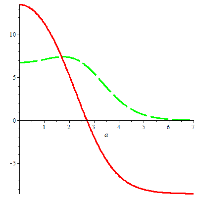
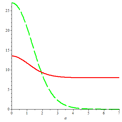
Figure 3: The figure displays the plots $\kappa_{c}^{-}$ vs $a$ and $\bar{\kappa}$ vs $a$ drawn by the solid and long-dashed lines correspondingly. For computing them, we have been applying the explicit expressions derived in example 1 to the specific signal profile $\tilde{f}(\eta)=\sin\eta$. The right (left) frame displays the plots drawn for $c=1/2$ ($c=3/2$). The case of homogeneous system corresponds to $a=0$. The values of the other parameters are as follows: $\delta=\nu=1$, $p_{e}=\beta=2/3$. For such parameters, $c_{*}=\sqrt{3/2}$ and $\kappa_{c}=\kappa_{*}=27/2$. Thus, $c>c_{*}$ ($c<c_{*}$) for the plots shown in the left (right) frame. For $a\to+0$, the limit value of $\bar{\kappa}$ is equal to $\kappa=2\kappa_{*}=27$ ($\kappa=\kappa_{*}/2=27/4$) for the right frame (left) frame. From what we have been saying above regarding stability and instability of the quasi-equilibria, it follows that the eigenmode with squared wavenumber $\beta=2/3$ associated to the quasi-equilibrium with the value of predator’s density equal to $p_{e}=2/3$ is unstable (stable) for every value of $a$ for which long-dashed line is above (below) the solid one. Hence we see in the left frame that the growth of $a$ destabilizes the eigenmode, which is stable for the values of $a$ close to zero. Further increase in $a$ entails the occurrence of the negative values of $\kappa_{c}^{-}$ (that causes the total destabilizing). In the right frame, we see that the growth of $a$ stabilizes the eigenmode, which is unstable for the values of $a$ close to zero.

5 Concluding remarks

We have been seeing exponential suppressing the predators’ motility in response to the growth of the signal amplitude. The natural treatment of this observation is that perceiving the intensive external signals distracts the predators from pursuing the prey. Given such an explanation, the effect might seem rather predictable, yet the exponential acuity of it remains surprising.

Intuitively, the loss of the predators’ motility could be enhancing the stability of the homogeneous quasi-equilibria and suppressing the excitation of waves but, generally speaking, this is not the case, see fig. 3. Indeed, increasing the amplitude of the external signal represented by a travelling wave gives rise to the total instability provided that the external wave speed is above the independent threshold defined by equality (4.23). Otherwise, the same action exerts the stabilizing effect, that becomes most pronounced in the limit case of the stationary waves.

In the end, increasing the amplitude of the external wave brings the system at almost degenerated form due to losing the motility. At that, the residual drift velocity becomes almost equal to that of the external wave. (Using the word ‘almost’ here indicates allowing the exponentially small deviations.) In the linear approximation, the degeneration reveals itself by the almost neutral waves propagating for every wavenumber at the phase velocities almost equal to the external wave speed. The instability relative to such waves seems to be very weak. However, they can interact non-linearly with the developed regimes which had been created by the local bifurcation at the smaller amplitude. (Imagine the threshold value of the motility decreasing and passing through the current value of the motility upon increasing the amplitude.)

The short-wavelength stabilization or destabilization of the quasi-equilibria resemble the effects of high-frequency vibration widely known in classical mechanics or the continuous media mechanics. The celebrated examples are the upside-down pendulum or the counterparts of it emergent from the dynamics of the stratified fluid. The vibrations translate their effect on such kind of systems via so-called effective potential energy, that arises upon averaging, see, e.g., articles by [20, 21]. Our examples show that the short-wavelength fluctuations of the environment exert their effects on the PKS systems quite differently, namely, by adding the drift. Studying the drift arising upon averaging the advection of some density by an oscillating velocity goes back to Stokes. Now this area is the subject of continuing researches. A reader can find more details and references, e.g., in the article by [22]. Usually, Stokes’ drift turns out to be relatively weak, and the effect of it reveals itself only regarding the long-term transport or mixing. Nevertheless, we have been observing stabilizing or destabilizing the quasi-equilibria only due to Stokes’s drift right in the leading approximation.

In our considerations, the unstable modes occur upon crossing the graphs of two critical values of motility denoted as $\kappa_{c}^{\pm}$. Right on each graph, there exists a neutral wave. The neutral wave occurring at the lower critical value equal to $\kappa_{c}^{-}$ propagates upstream, i.e. faster than the residual drift, and the other one propagates downstream, i.e. slower than the residual drift. Since the value of $\kappa_{c}^{-}$ is the stability threshold, the wave propagating upstream destabilizes the quasi-equilibria. When the residual drift vanishes, the upper and lower critical motilities collide and merge with that reported in the case of equilibria. These features are due to breaking the reflectional symmetry by the drift. In particular, the double neutral mode existing due to the reflectional symmetry splits itself into two simple ones. Thus we arrive at a two-parametric phenomenon that deserves detailed nonlinear analysis.

Considering the PKS systems in the bounded spatial domains allows us to avoid some difficulties emergent from the continuous spectra, but brings us at the problem of choosing the boundary conditions. For instance, imposing the Neumann conditions as done in the cited articles leads to some technical issues upon homogenizing the problem and even upon doing the linear analysis. Addressing these technicalities does not seem to be essential since it is not clear whether the Neumann conditions are less artificial than the others. Besides, reducing the symmetry by the boundary conditions can cut out some solutions. In such circumstances, the softer conditions of spatial periodicity seem to be the best. Under such conditions, the homogeneous system (1.4)-(1.6) and more general PKS systems possess the translational and mirror symmetries. Although it doubles the neutral modes, the corresponding bifurcations can be addressed using the general theory given in article [26].

Two more apparent topics for continuing the present research are the short standing waves and the slowly modulated travelling waves. For instance, the functions $f=A\sin\tau\sin\xi$ and $f=A\sin t\sin(\xi-c\tau)$ stand as the representatives of the former and the latter kinds correspondingly. Both classes of signals produce the homogeneous quasi-equilibria but the coefficients of the homogenized system become variable. In the case of time-periodic slow modulation, one can address the corresponding spectral stability problem using Floquet’s theory.

Finally, it is of interest to what extent the shape of the external signal influences its effect. In particular, there arises an interesting optimization problem for the effective motility defined in (4.18) or in (4.24) subject to restriction $\langle f^{2}\rangle=1.$

Acknowledgments

Andrey Morgulis acknowledges the support from Southern Federal University (SFedU)

6 Appendix I. Derivation of the asymptotics

In this appendix, we derive formally the asymptotic approximation described in Sec. 2.

Introducing the fast variables $\xi=\omega x$, $\tau=\omega t$ into the governing equations (1.4)-(1.6) puts them into the following form

$$\omega((\partial_{t}+\omega\partial_{\tau})u-(\partial_{x}+\omega\partial_{\xi})(\kappa q+f)+\nu u)=\nu_{1}(\partial_{x}+\omega\partial_{\xi})^{2}u;$$ (6.1)

$$\omega((\partial_{t}+\omega\partial_{\tau})p+(\partial_{x}+\omega\partial_{\xi})(up))=\nu_{2}(\partial_{x}+\omega\partial_{\xi})^{2}p;$$ (6.2)

$$(\partial_{t}+\omega\partial_{\tau})q-q(1-p-q)=\delta_{q}(\partial_{x}+\omega\partial_{\xi})^{2}q.$$ (6.3)

We look for an asymptotic expansion of the solution to system (6.1)-(6.3) that reads as

$$(u,p,q)=\sum_{k\geqslant 0}\omega^{-k}(u_{k},p_{k},q_{k})(x,t,\xi,\tau),\omega\to\infty.$$ (6.4)

We require all the coefficients of series (6.4) to be $2\pi-$periodic in $\xi$ and $\tau$. Replacing the unknowns of system (6.1)-(6.3) by series (6.4) and collecting the terms of equal order in $\omega$ yield a sequence of equations, which we will be solving step by step.

Collecting the terms of order $\omega^{2}$ in equation (6.3) leads to the equation

$$\partial_{\xi\xi}q_{0}=0.$$ (6.5)

There are no periodic solutions to equation (6.5) except for those independent of $\xi$. Hence

$$q_{0}={q}_{0}(x,t,\tau).$$ (6.6)

Function ${q}_{0}$ remains unknown to us, and we have to determine it at the subsequent steps. Given the equality (6.6), collecting the terms of order $\omega^{2}$ in equations (6.1-6.2) leads to the equations

$$(\partial_{\tau}-\nu_{1}\partial_{\xi\xi})u_{0}=\partial_{\xi}f;$$ (6.7)

$$(\partial_{\tau}-\nu_{2}\partial_{\xi\xi})p_{0}+\partial_{\xi}(u_{0}p_{0})=0;$$ (6.8)

$$(u_{0},p_{0})=(u_{0},p_{0})(x,t,\xi,\tau),\ (\xi,\tau)\in\mathbb{T}^{2}.$$

Note that equation (6.7) is exactly the first equation in problem (2.7). Equation (6.7) has only one periodic solution vanishing on average in the sense of definition (2.1). We denote this solution as $\tilde{u}_{0}$. Thus $u_{0}=\bar{u}+\tilde{u}_{0}$, $\bar{u}=\langle u_{0}\rangle$, and we have justified the leading term in the asymptotic approximation for $u$ given by (2.5), (2.7).

We need the following
Lemma. Let $w=w(\xi,\tau)$ be a smooth function on $\mathbb{T}^{2}$. Consider equation

$$\partial_{\tau}Q+\partial_{\xi}(wQ-{\epsilon}\partial_{\xi}Q)=0\ \text{on}\ \mathbb{T}^{2};\ {\epsilon}=\operatorname{const}>0.$$ (6.9)

Then there exists a unique $2\pi$-periodic (in $\xi$ and $\tau$) solution to equation (6.9) satisfying the additional condition

$$\langle Q\rangle=1.$$ (6.10)

We’ll prove this assertion at the end of this Appendix.

We continue constructing the asymptotic expansion. By the above lemma, problem (2.8) has a unique solution $P=P(x,t,\xi,\tau)$. Hence every solution to equation (6.8) reads as

$$p_{0}=\bar{p}(x,t)P(x,t,\xi,\tau).$$ (6.11)

Thus we have got the leading term of asymptotic approximation (2.6) for unknown $p$.

Now let us consider the terms of order $\omega$. It follows from equations (6.3) and (6.6) that

$$\delta_{q}\partial_{\xi\xi}q_{1}=\partial_{\tau}q_{0}.$$ (6.12)

Since function $q_{0}$ does not depend on $\xi$, equation (6.12) has a periodic solution if and only if function $q_{0}$ does not depend on $\tau$. Hence $q_{0}=\bar{q}(x,t)$ and we get the leading term of asymptotic approximation (2.4) for unknown $q$. Further, every solution to equation (6.12) reads as

$$q_{1}=q_{1}(x,t,\tau).$$ (6.13)

Functions $q_{1}$ and $\bar{q}$ remains unknown to us, and we have to determine them at the subsequent steps. Note that the existence of a periodic solution to equation (6.12) justifies the error estimate (i.e. $O-$ term) of asymptotic approximation (2.4).

Given the equality (6.13), collecting the terms of order $\omega$ in equation (6.1)-(6.2) leads to the following equations

$$(\partial_{\tau}u_{1}-\nu_{1}\partial_{\xi\xi})u_{1}=2\nu_{1}\partial_{x\xi}u_{0}+\partial_{x}(\kappa q_{0}+f)-\nu u_{0}-\partial_{t}u_{0},\quad(\xi,\tau)\in\mathbb{T}^{2};$$ (6.14)

$$\partial_{\tau}p_{1}+\partial_{\xi}(u_{0}p_{1})-\nu_{2}\partial_{\xi\xi}p_{1}=2\nu_{2}\partial_{x\xi}p_{0}-\partial_{t}p_{0}-\partial_{x}(u_{0}p_{0})-\partial_{\xi}(u_{1}p_{0}),\quad(\xi,\tau)\in\mathbb{T}^{2}.$$ (6.15)

Averaging equations (6.14) and (6.15) while keeping in mind equality (6.11) brings us at equations (2.9)-(2.10). Similarly, proceeding with equation (6.3), we get equation (2.11), that completes the homogenized system consisting of equations (2.9)-(2.11). Resolving the homogenized system implies the existence of periodic solutions to equations (6.14) and (6.15), which, in turn, justifies $O-$terms of the asymptotic approximations (2.5) and (2.6)).

Now we pass to proving the lemma. Let $\mathrm{H}$ be the space of the Fourier series in $\xi,\tau$ with square-summable coefficients and let $\mathcal{L}:\mathrm{H}\to\mathrm{H}$ be operator defined by the left-hand side of equation (6.9). We have to prove that

$$\dim\,\mathrm{Ker}\,\mathcal{L}=1,\ \langle\chi\rangle\neq 0\ \forall\ \chi\in\mathrm{Ker}\,\mathcal{L}\setminus\{0\}.$$ (6.16)

Let $\mathcal{L}^{*}$ denote the operator adjoint to $\mathcal{L}$ and let $\mathcal{J}:\mathrm{H}\to\mathrm{H}$ be the action of inversion $(\xi,\tau)\mapsto(-\xi,-\tau)$. Define

$$\breve{\mathcal{L}}^{*}=\mathcal{{J}}\mathcal{L}^{*}\mathcal{{J}}$$

Then

$$\breve{\mathcal{L}}^{*}:\varphi\mapsto(\partial_{\tau}-{\epsilon}\partial_{\xi\xi})\varphi+w\partial_{\xi}\varphi.$$

Notice that PDE

$$(\partial_{\tau}-{\epsilon}\partial_{\xi\xi})\varphi+w\partial_{\xi}\varphi=0$$

obeys the strong maximum and minimum principles (see, e.g. [28] or [29]). Hence

$$\mathrm{Ker}\,\breve{\mathcal{L}}^{*}=\{\varphi\equiv\operatorname{const}\}=\mathrm{Ker}\,\mathcal{L}^{*}.$$

Applying the unilateral strong maximum/minimum principles to PDE

$$(\partial_{\tau}-{\epsilon}\partial_{\xi\xi})\varphi+w\partial_{\xi}\varphi=1$$

shows that neither equation $\breve{\mathcal{L}}^{*}\breve{\psi}=1$ nor equation ${\mathcal{L}}^{*}\psi=1$ has a solution belonging to $\mathrm{H}$. Consequently, the resolvent $(\mathcal{L}^{*}-\lambda\mathcal{I})^{-1}$, $\lambda\in\mathbb{C}$, has a simple pole at the origin. Since this resolvent is compact, the pair of operators $\mathcal{L}^{*}$ and $\mathcal{L}$ obeys the Fredholm theorems. Hence $\dim\,\mathrm{Ker}\,\mathcal{L}=1$. Furthermore, conjecturing that $\langle\chi\rangle=0$ for some $\chi\in\mathrm{Ker}\,\mathcal{L}\setminus\{0\}$ would imply the existence of solution to equation $\mathcal{L}^{*}\psi=\operatorname{const}\neq 0$ but this contradicts to what we have proved above. This completes the proof.

Remark 6

Let $\Pi^{*}$ denote spectral projector onto $\mathrm{Ker}\,\mathcal{L}^{*}$. Let $\Pi^{*}(\sigma)$ denote the family of such projectors induced by the conjugated to equation (2.13). Then the action of mapping (2.12) is identical to $\eta\mapsto\langle\Pi^{*}(\sigma)\tilde{u}_{0}\rangle$. Hence the perturbation theory for the linear operators implies that this mapping is differentiable and even analytic in the vicinity of origin. Therefore, the drift operator is analytic too by the definition of it by equality (2.14), and the derivatives of it can be evaluated using equalities (4.10)-(4.11).

7 Appendix II. Linear stability.

In this appendix, we put the details of the linear stability analysis of the equilibria and quasi-equilibria.

7.1 Equlibria

Let us choose an equilibrium out of family (3.2) by specifying the value of the family parameter denoted as $p_{e}$. The eigenvalues corresponding to eigenmode (4.4) having a specific wavenumber $\alpha$ are solutions to the following algebraic equation

$$\lambda^{3}+(D_{1}+D_{2}+D_{3})\lambda^{2}+(D_{2}D_{3}+D_{1}D_{3}+D_{1}D_{2})\lambda+D_{1}D_{2}D_{3}+\beta\kappa p_{e}q_{e}=0,$$ (7.1)

$$D_{1}=\nu+\beta\delta_{u};\ D_{2}=\beta\delta_{p};\ D_{3}=q_{e}+\beta\delta_{q};\ \beta=\alpha^{2},\ p_{e}+q_{e}=1$$

By restrictions (4.5), all the coefficients of the polynomial on the left-hand side of equation (7.1) are strictly positive. Consequently, the roots of this polynomial are neither positive nor zero. Hence neither unstable nor neutral eigenmode corresponds to a real eigenvalue.

It follows from the Routh-Hurwitz theorem that the necessary and sufficient condition for belonging all the roots of polynomial (7.1) to the open left half-plane of the complex plane reads as

$$(D_{1}+D_{2}+D_{3})(D_{2}D_{3}+D_{1}D_{3}+D_{1}D_{2})>D_{1}D_{2}D_{3}+\beta\kappa p_{e}q_{e}.$$

This inequality allows a more compact form, namely:

$$(D_{1}+D_{2})(D_{1}+D_{3})(D_{2}+D_{3})>\beta\kappa p_{e}q_{e}.$$

Since the degree of polynomial (7.1) is 3, replacing the last inequality by equality is necessary and sufficient for belonging the root of the polynomial (7.1) to the imaginary axis, and this root cannot be zero. Given this observation, we conclude that the critical magnitude of predators’ motility discussed in section 4.1 has the following form

$$\kappa_{c}=\frac{(D_{1}+D_{2})(D_{1}+D_{3})(D_{2}+D_{3})}{\beta p_{e}q_{e}}.$$ (7.2)

In the case of $\delta_{u}=\delta_{p}=0$, which is of particular interest for the considerations of section 4.2, expression (7.2) simplifies to

$$\kappa_{c}^{0}=\kappa_{c}|_{\delta_{p}=\delta_{u}=0}={\frac{{\nu}\,\left({\delta_{q}}\,\beta+{\nu}+q_{e}\right)\left({\delta_{q}}\,\beta+q_{e}\right)}{q_{e}\,p_{e}\beta}}.$$ (7.3)

The direct inspection using the expression  (7.2) or (7.3) shows the positiveness of the threshold value of motility denoted as $\kappa_{*}(\delta)$ in section 4.1. For instance,

$$\left.\kappa_{*}(\delta)\right|_{\delta=(1,1,0,0)}=27/2.$$

7.2 Quasi-equilibria

Given the external signal having the form of travelling wave (4.12), we analyze the linear stability of a homogeneous quasi-equilibrium. Then the small perturbations of it obey system (4.13)-(4.14), all the coefficients of which are constant. Acting the same way as in the case of equilibria, we arrive at the characteristic polynomial, that reads as

$${\lambda}^{3}+\left(iU+\nu+q_{e}+\delta_{q}\beta\right){\lambda}^{2}+\left(\left(iU+q_{e}+\delta_{q}\beta\right)\nu+iU(q_{e}+\delta_{q}\beta)\,\right)\lambda+i\nu U(q_{e}+\delta_{q}\beta)\,+\beta p_{e}q_{e}\bar{\kappa}.$$

Here $\beta=\alpha^{2}$, $\alpha$ stands for the eigenmode wavenumber, $U=\alpha v_{e}$, $v_{e}$ stands for the drift velocity determined by equality (2.29), and $\bar{\kappa}=(1+\mathcal{V}^{\prime}(f))\kappa$ is the effective motility determined by equality (4.24). For the sake of convenience, we write this polynomial in more compact form, namely,

$${\lambda}^{3}+\left(iU+d_{1}\right){\lambda}^{2}+\left(d_{2}+iUd_{1}\,\right)\lambda+iUd_{2}\,+r$$

where

$$d_{1}=\nu+q_{e}+\delta_{q}\beta,\ d_{2}=\nu(q_{e}+\delta_{q}\beta),\ r=\beta p_{e}q_{e}\bar{\kappa}.$$

Note that $r>0$, $d_{1}>0$ and $d_{2}>0$ for every admissible set of the problem parameters.

We employ the complex-valued version of Hurwitz’s theorem to count the roots belonging to the right complex semi-plane, and it brings us at the chain of the Hankel’s matrix minors, that reads as

$$1,\ d_{1},\ d_{1}\left(d_{2}d_{1}-r\right),\ r\left((r-d_{1}d_{2})^{2}-{U}^{2}{{d_{1}}}^{2}{d_{2}}\right).$$

For this chain, there are four generic distributions of signs of the minors, namely

$$++++,\quad+++-,\quad++--,\quad++-+.$$

Switching between the diagrams displayed herein corresponds to crossing certain critical submanifolds in the space of the problem parameters. These are the null sets of functions $\bar{\kappa}-\kappa_{c}^{(j)}(v_{e},p_{e},\beta,\delta)$, $j\in\{+,-,0\}$, where $\kappa_{c}^{(0)}$ is the critical motility defined by equality (7.3), and

$$\kappa_{c}^{(\pm)}=\frac{c_{*}d_{1}(c_{*}\pm|v_{e}|)}{p_{e}q_{e}},\ c_{*}=\sqrt{{d_{2}}/{\beta}},$$ (7.4)

Note that $\kappa_{c}^{-}<\kappa_{c}^{0}<\kappa_{c}^{+}$ for every admissible set of the problem parameters provided that $v_{e}\neq 0$. If $v_{e}=0$ then $\kappa_{c}^{-}=\kappa_{c}^{0}=\kappa_{c}^{+}$. Therefore, passing the effective motility through the values of $\kappa_{c}^{-}$, $\kappa_{c}^{0}$, and $\kappa_{c}^{+}$ in the ascending order causes switching between the above diagrams from left to right provided that the values of all other parameters stay unaltered. Hence the number of roots in the right complex semi-plane takes the values of 0,1 and 2 provided that the value of $\bar{\kappa}$ belongs to intervals $(0,\kappa_{c}^{-})$, $(\kappa_{c}^{-},\kappa_{c}^{+})$ and $(\kappa_{c}^{+},\infty)$ correspondingly. Changing this number is due to changing the sign of the senior minor of Hankel’s matrix. Therefore, passing the effective motility through one of the values of $\kappa_{c}^{\pm}$ causes crossing the imaginary axis by the root of the characteristic polynomial at some non-zero point. Hence the oscillatory instability occurs at this moment. Note that passing through the value of $\kappa_{c}^{0}$ does not change the number of unstable roots.

For $\kappa=\kappa^{\pm}_{c}$ and $v_{e}>0$ the neutral eigenmode is proportional to

$$\mathrm{e}^{i\sqrt{\beta}(x\pm c_{*}t)},$$

and every eigenmode appears together with the complex-conjugated one. For $v_{e}<0$, it suffices to substitute $x\pm c_{*}t$ by $x\mp c_{*}t$.

Remark 7

Inequalities $|v_{e}|\gtrless c_{*}$ are equivalent to $\kappa_{c}^{-}\lessgtr 0$. Occurring the negative values of $\kappa_{c}^{-}$ for a specific wavelength excludes the diagram $++++$. Hence the eigenmode with such a wavelength is unstable for every quasi-equilibrium.

8 Appendix III. Estimates of exponential integrals.

In this appendix, we estimate the integrals introduced in (2.26) and denoted as $\Gamma_{\pm}$ when the signal amplitude denoted as $a$ tends to infinity. For simplicity, we restrict ourselves within the class of the unmodulated travelling waves defined by equality (4.12). Then $\Gamma_{\pm}=\Gamma_{\pm}(z),\ z\gtrless 0$. For definiteness, let’s consider $\Gamma_{+}=\Gamma_{+}(z),z>0$. We put this integral into a slightly different form that is more convenient for applying the Laplace method, namely,

$$\frac{1}{2\pi}\int\limits_{(0,\infty)\times(0,2\pi)}\mathrm{e}^{-z\sigma}\mathrm{e}^{aS(\eta,\sigma)}d\eta d\sigma,\quad S(\eta,\sigma)=s(\eta)-s(\eta-\sigma),\ z>0$$ (8.1)

For simplicity, we consider function $s$ as a given one, and we assume that it is $2\pi-$periodic, vanishing on average and analytic and that every critical point of it is non-degenerated. The periodicity allows us to reduce the domain of integration of integral (8.1) to cylinder

$$C=\{(\eta,\sigma)\in\mathbb{S}\times(0,2\pi)\},$$

and we arrive at estimating the following integral

$$\int\limits_{C}\mathrm{e}^{-{z}\sigma}\mathrm{e}^{aS(\eta,\sigma)}d\eta d\sigma.$$ (8.2)

The local maximizers of $S$ on the whole $(\eta,\sigma)-$plain are

$$(\eta,\sigma)\in\mathbb{R}^{2}:\ s^{\prime}(\eta)=s^{\prime}(\eta-\sigma)=0,\quad s^{\prime\prime}(\eta)s^{\prime\prime}(\eta-\sigma)<0.$$

The last inequality means that no maximizers belong to ${\partial}C$. Then the leading term in Laplace’s asymptotics of integral (8.2) for $a\to\infty$ reads as

$$\frac{2\pi\mathrm{e}^{a\mathrm{osc}(s)}}{a}\sum\limits_{(x,y)\in M}\frac{\mathrm{e}^{-{z}(x-y)}}{\sqrt{-s^{\prime\prime}(x)s^{\prime\prime}(y)}}$$

where

$$\mathrm{osc}(s)=\sup\limits_{\mathbb{R}}s-\inf\limits_{\mathbb{R}}s,\quad M=\{(x,y):\ 0<x\leq 2\pi,0<x-y<2\pi,\mathrm{osc}(s)=s(x)-s(y)\}.$$ (8.3)

Coming back to the integral (8.1) brings us at the following estimate

$$\Gamma_{+}(z)\sim\frac{\mathrm{e}^{a\mathrm{osc}(s)}}{a(1-\mathrm{e}^{-2\pi{z}})}\sum\limits_{(x,y)\in M}\frac{\mathrm{e}^{-{z}(x-y)}}{\sqrt{-s^{\prime\prime}(x)s^{\prime\prime}(y)}},\quad a\to\infty.$$ (8.4)

Example 5

Let $s(\eta)=\sin\eta$. Then $\mathrm{osc}(s)=2$, $M=\{(\pi/2,-\pi/2)\}$, and estimate (8.4) reads as

$$\Gamma_{+}(z)\sim\frac{\mathrm{e}^{2a}\mathrm{e}^{-\pi{z}}}{a(1-\mathrm{e}^{-2\pi{z}})},\quad a\to\infty.$$

Remark 8

Asymptotics (8.4) delivers an estimate for the residual drift velocity that we have been defining by equality (2.33) involving the value of $\Gamma_{+}$ for $z=c/\nu_{2}$. This estimate matches the limit identity (2.34). In particular, using the estimate of example 5 for $z\to+0$ bring us at the leading term in the asymptotics of function $I^{2}_{0}(a)$, $a\to\infty$, in consistence with what we have learned from the example 4. Note finally that differentiating the asymptotics of $\Gamma_{+}$ gives us the effective motility factor defined by equality (4.24).

References

- [1] Ivanitskii GR, Medvinskii AB, Tsyganov, MA. (). From the dynamics of population autowaves generated by living cells to neuroinformatics. Physics-Uspekhi 1994; 37(10): 961.
- [2] Tsyganov MA, Brindley J, Holden AV., Biktashev VN. Quasisoliton interaction of pursuitevasion waves in a predator-prey system.Phys. Rev. Lett. 2003; 91(21): 218102-1-4.
- [3] Tsyganov MA, Brindley J, Holden AV, Biktashev VN. Soliton-like phenomena in one-dimensional cross-diffusion systems: a predator–prey pursuit and evasion example. Physica D: Nonlinear Phenomena 2004; 197(1-2): 18-33.
- [4] Tsyganov MA, Biktashev VN. Half-soliton interaction of population taxis waves in predator-prey systems with pursuit and evasion. Physical Review E 2004 70(3): 031901.
- [5] Govorukhin V, Morgulis A, Tyutyunov Y. Slow taxis in a predator-prey model. Doklady Mathematics 2000; 61(3): 420-422.
- [6] Arditi R, Tyutyunov Y, Morgulis A, Govorukhin V, Senina I. Directed movement of predators and the emergence of density-dependence in predator–prey models. Theoretical Population Biology 2001; 59(3): 207-221.
- [7] Pearce IG, Chaplain MAJ, · Schofield PG, Anderson ARA, Hubbard SF. Chemotaxis-induced spatio-temporal heterogeneity in multi-species host-parasitoid systems. J. Math. Biol. 2007; 55(3): 365–388.
- [8] Bellomo N,Bellouquid A, Tao Y, Winkler M. Toward a mathematical theory of Keller-Segel models of pattern formation in biological tissues. Math. Models Methods Appl. Sci. 2015; 25(09): 1663-1763.
- [9] Li C, Wang X, Shao Y. Steady states of a predator–prey model with prey-taxis. Nonlinear Analysis: Theory, Methods and Applications. 2014. 97: 155-168.
- [10] Tello IJ , Wrzosek D. Predator–prey model with diffusion and indirect prey-taxis. Math. Models Methods Appl. Sci. 2016; 26(11): 2129-2162.
- [11] Tyutyunov Y, Titova L, Senina I. Prey-taxis destabilizes homogeneous stationary state in spatial Gause–Kolmogorov-type model for predator–prey system. Ecological Complexity 2017; 31: 170-180.
- [12] Wang Q, Yang J, Zhang L. Time-periodic and stable patterns of a two-competing-species Keller-Segel chemotaxis model: Effect of cellular growth. Discrete & Continuous Dynamical Systems - B. 2017; 22(9):3547-3574.
- [13] Li U, Tao Y. Boundedness in a chemotaxis system with indirect signal production and generalized logistic source. Appl. Math. Letters 2018; 77: 108-113.
- [14] Yurk BP, Cobbold CA. Homogenization techniques for population dynamics in strongly heterogeneous landscapes. Journal of Biological Dynamics 2018; 12(1): 171-193.
- [15] Black T. Boundedness in a Keller–Segel system with external signal production. Journ. of Math. Analysis Appl. 2017; 446(1): 436-455.
- [16] Issa, T.B. & Shen, W. J. Dyn. Diff. Equat. (2018) https://doi.org/10.1007/s10884-018-9686-7
- [17] Iooss, G., & Joseph, D. D. (2012). Elementary stability and bifurcation theory. Springer Science & Business Media.
- [18] Arnold, V. I., Afrajmovich, V. S., Il’yashenko, Y. S., & Shil’nikov, L. P. (2013). Dynamical systems V: bifurcation theory and catastrophe theory (Vol. 5). Springer Science & Business Media.
- [19] Haragus, M., & Iooss, G. (2010). Local bifurcations, center manifolds, and normal forms in infinite-dimensional dynamical systems. Springer Science & Business Media..
- [20] Yudovich V. The dynamics of vibrations in systems with constraints. Doklady Physics 1997; 42, 322-325.
- [21] Vladimirov V. On vibrodynamics of pendulum and submerged solid. Journ. of Math. Fluid Mech. 2005; 7 (S3): S397-S412.
- [22] Vladimirov V. Two-Timing Hypothesis, Distinguished Limits, Drifts, and Pseudo-Diffusion for Oscillating Flows. Studies in Appl. Math. 2017; 138(3): 269-293.
- [23] Allaire. G. A brief introduction to homogenization and miscellaneous applications. ESAIM: Proceedings. Vol. 37. EDP Sciences; 2012.
- [24] Allaire G. Homogenization and two-scale convergence. SIAM Journal on Math. Analysis 1992; 23(6): 1482-1518.
- [25] G. Allaire. Shape optimization by the homogenization method. Vol. 146. Springer Science & Business Media; 2012.
- [26] Morshneva I. & Yudovich, V. (). Bifurcation of cycles from equilibria of inversion-and rotation-symmetric dynamical systems. Sib. Math. J. 1985, 26(1): 97-104.
- [27] Yudovich, V. Cycle-creating bifurcation from a family of equilibria of a dynamical system and its delay, J. Appl. Math. Mech. 1998, 62 (1): 19-29. https://doi.org/10.1016/S0021-8928(98)00002-1.
- [28] Nirenberg L. A strong maximum principle for parabolic equations. Comm. Pure Appl. Math. 1953; 6(2): 167-177.
- [29] Landis EM. Second order equations of elliptic and parabolic type. American Math. Soc.; 1997.