Non-perturbative approaches to the quantum Seiberg–Witten curve

Abstract

We study various non-perturbative approaches to the quantization of the Seiberg–Witten curve of ${\cal N}=2$, $SU(2)$ super Yang–Mills theory, which is closely related to the modified Mathieu operator. The first approach is based on the quantum WKB periods and their resurgent properties. We show that these properties are encoded in the TBA equations of Gaiotto–Moore–Neitzke determined by the BPS spectrum of the theory, and we relate the Borel-resummed quantum periods to instanton calculus. In addition, we use the TS/ST correspondence to obtain a closed formula for the Fredholm determinant of the modified Mathieu operator. Finally, by using blowup equations, we explain the connection between this operator and the $\tau$ function of Painlevé $\rm III$.

1 Introduction

In recent years, many interesting and surprising relations have been obtained between quantum mechanical systems, on one hand, and supersymmetric gauge theories and topological strings, on the other hand. One example of such a relation is the gauge/Bethe correspondence of ns , which connects quantum integrable systems to instanton calculus in gauge theory. A second example is the topological string/spectral theory (TS/ST) correspondence, which provides explicit predictions for the spectral determinants of quantum mirror curves ghm ; cgm ; mmrev . Finally, the study of BPS states in supersymmetric gauge theories turns out to be closely related to the WKB method as applied to Seiberg–Witten (SW) curves gmn ; gmn2 ; oper . This relation can be upgraded to include resurgent properties of the quantum periods ims ; mm-s2019 . All these connections can be used to obtain new results in quantum theory from gauge/string theory. For example, the results of ns ; ghm lead to new exact quantization conditions for the spectrum of the relevant operators. Conversely, one can use quantum mechanical results to derive new results of string/gauge theories, like for example non-perturbative definitions of topological string partition functions on local Calabi–Yau (CY) manifolds ghm ; cgm ; mz .

Perhaps the simplest quantum-mechanical model where all these methods can be applied is the quantum version of the SW curve for ${\cal N}=2$, $SU(2)$ super Yang–Mills (SYM) theory. The corresponding operator is the (modified) Mathieu operator, which is a traditional chapter in the theory of Schrödinger operators. This operator has been also revisited in the context of supersymmetric gauge theory and topological string theory in various works (see e.g. mirmor ; he-miao ; huangNS ; basar-dunne ; kpt ; ashok ; coms ), but many important aspects have not been discussed yet. In this paper we use methods from supersymmetric gauge theory and topological string theory to obtain quantum-mechanical properties of the modified Mathieu operator at the non-perturbative level, and we test these properties against first-principles computations. We also discuss the relationships between these different approaches.

The first aspect that we explore is the resurgent structure of the quantum periods, which we review in section 2. Building on gmn2 , Gaiotto considered in oper the conformal limit of the TBA equations of gmn for an ${\cal N}=2$ supersymmetric gauge theory, and he conjectured that the resulting integral equations describe the quantum periods for the corresponding quantum SW curve. In the case of Argyres–Douglas theories, this problem was studied in detail in ims , which pointed out precise connections to the resurgent properties of these periods, and used these properties to derive the conjecture of oper in the case of general polynomial potentials

In section 3 of this paper we use the conformal limit of the TBA equations to obtain a prediction for these resurgent properties in the case of the modified Mathieu operator. In particular, we obtain the precise structure of the Stokes discontinuities of the quantum periods. We then test these predictions against first-principles calculations in the all-orders WKB method, in particular against high order results for the expansion of the quantum periods. We also comment on how to use these TBA equations to compute Borel resummations of the quantum periods.

As pointed out in mirmor and explored in many subsequent papers, the NS limit of instanton calculus ns provides a different resummation of the WKB expansion, in terms of a convergent expansion in the instanton counting parameter. However, this resummation has a very different flavor from the Borel resummation appearing in the theory of resurgence, and it is important to have a precise dictionary between the two types of resummation. We address this issue in section 4.

As we mentioned above, the TS/ST correspondence gives explicit expressions for spectral determinants of operators obtained in the quantization of mirror curves. As pointed out in gm3 , there is a four-dimensional limit of the correspondence in which the relevant operator is the quantization of the SW curve for pure ${\cal N}=2$, $SU(N)$ Yang–Mills theory. This leads to a spectral problem which is different from the one considered in ns for $N>2$. In the case of the $SU(2)$ theory considered in this paper, the spectral problems coincide, but the TS/ST correspondence gives, in addition to the quantization condition of ns , an explicit expression for the spectral determinant, which we derive in detail in section 5 of this paper. The resummed quantum periods defined by instanton calculus are key ingredients in this expression. We test the resulting formula and in particular we compare our result to the TBA equation describing this spectral determinant which was conjectured by Al. B. Zamolodchikov in post-zamo .

In section 6, based on previous works, we use the vanishing Nakajima-Yoshioka blowup equations to prove that the exact spectrum of the modified Mathieu operator is computed by the zeros of the $\tau$ function of Painlevé $\rm III_{3}$. Finally, in section 7 we conclude and discuss some open problems.

We have also included two Appendices: in the first one we extend the derivation of section 5 to $SU(N)$ quantum SW curves, while in the second one we review some of the results of Zamolodchikov’s paper post-zamo .

2 The all-orders WKB method

Our first approach to the quantum SW curve will be based on the so-called exact WKB method, see for example voros ; voros-quartic ; ddpham ; in-exactwkb . We will now summarize the basic ingredients of the theory.

The Schrödinger equation for a non-relativistic particle in a potential $V(x)$ and with energy $E$ reads as follows:

$$-\hbar^{2}\psi^{\prime\prime}(x)+(V(x)-E)\psi(x)=0.$$ (2.1)

The standard WKB method produces asymptotic expansions in $\hbar$ for the solutions to this equation. Let us consider the following ansatz for the wavefunction,

$$\psi(x)=\exp\left(\frac{{\rm i}}{\hbar}\int^{x}Y(x^{\prime},E;\hbar){\rm d}x^{\prime}\right)\ .$$ (2.2)

The function $Y(x,E;\hbar)$ satisfies the Riccati equation

$$Y^{2}-{\rm i}\hbar\frac{{\rm d}Y}{{\rm d}x}=E-V(x)\ .$$ (2.3)

It has the formal power series expansion in powers of $\hbar$

$$Y(x,E;\hbar)=\sum_{n=0}^{\infty}p_{n}(x,E)\hbar^{n}\ ,$$ (2.4)

where in particular $p_{0}(x,E)$ is the classical momentum as a function of $x$ and the conserved energy. If one splits $Y$ into the even component and the odd component,

$$Y=p_{\text{even}}+p_{\text{odd}},$$ (2.5)

with

$$p_{\text{even}}(x,E;\hbar)=\sum_{n=0}^{\infty}p_{2n}(x,E)\hbar^{2n}\ ,\quad p_{\text{odd}}(x,E;\hbar)=\sum_{n=0}^{\infty}p_{2n+1}(x,E)\hbar^{2n+1}\ ,$$ (2.6)

one finds that the odd component is in fact a total derivative

$$p_{\text{odd}}(x,E;\hbar)=\frac{{\rm i}\hbar}{2}\frac{{\rm d}}{{\rm d}x}\log p_{\text{even}}(x,E;\hbar).$$ (2.7)

By substituting (2.2) into the Schrödinger equation, one finds (see for instance bpv )

$$p_{2n}=(-1)^{n}v_{2n}\ ,\quad n\geq 0$$ (2.8)

$$v_{n}=\frac{1}{2p_{0}}\left(\partial_{x}v_{n-1}-\sum_{k=1}^{n-1}v_{k}v_{n-k}\right)\ ,$$ (2.9)

from which the components $p_{2n}(x,E)$ can be solved recursively, starting from the known expression of $p_{0}$.

Geometrically, we can regard $p_{\rm even}(x,E;\hbar){\rm d}x$ as a meromorphic differential on the curve defined by

$$y^{2}=2(E-V(x)).$$ (2.10)

We will call it the WKB curve, and we will denote it as $\Sigma_{\rm WKB}$. This curve depends on a set of moduli which include the energy $E$ and the parameters of the potential $V(x)$. The basic objects in the exact WKB method are the periods of $p_{\rm even}(x,E;\hbar){\rm d}x$ along one-cycles of $\Sigma_{\rm WKB}$, which we will call WKB periods or quantum periods. We will denote them as

$$\Pi_{\gamma}(\hbar)=\oint_{\gamma}p_{\rm even}(x,E;\hbar){\rm d}x,\qquad\gamma\in H_{1}(\Sigma_{\rm WKB}),$$ (2.11)

and they are formal power series in even powers of $\hbar$, just like $p_{\rm even}(x)$,

$$\Pi_{\gamma}(\hbar)=\sum_{n\geq 0}\Pi^{(n)}_{\gamma}\hbar^{2n},\qquad\Pi^{(n)}_{\gamma}=\oint_{\gamma}p_{n}(x,E){\rm d}x.$$ (2.12)

Note that the coefficients $\Pi^{(n)}_{\gamma}$ depend on the moduli of the WKB curve. We will call $\Pi^{(0)}_{\gamma}$ the classical periods. The calculation of these coefficients at high order can be quite involved, even for simple quantum systems.

In this paper we are interested in the modified Mathieu Hamiltonian, with the conventions

$$H(p,x)=p^{2}+V(x),\qquad V(x)=2\Lambda^{2}\cosh x.$$ (2.13)

Upon quantization, we obtain the operator

$$\mathsf{H}=\mathsf{p}^{2}+2\Lambda^{2}\cosh(\mathsf{x}),\qquad[\mathsf{x},\mathsf{p}]={\rm i}\hbar.$$ (2.14)

We will refer to this as the modified Mathieu operator. It is well-known that the WKB curve of the modified Mathieu Hamiltonian happens to coincide with the SW curve of ${\cal N}=2$, $SU(2)$ Yang–Mills theory, in the conventions appropriate for the relation to integrable systems (see e.g. lerche-rev for a review of SW theory and swbook for its connection to integrable systems). In order to do this, we identify $E$ with the Coulomb modulus $u$ by

$$E=2u\ .$$ (2.15)

Let us first consider the classical periods of the modified Mathieu equation. Since the WKB curve is a torus, there will be two periods, corresponding to the two cycles of the torus. The $B$ period corresponds to the classical volume of phase space

$$\Pi_{B}^{(0)}(E)=4\,{\rm i}\int_{0}^{x_{+}}{\rm d}x\,\sqrt{E-2\Lambda^{2}\cosh x},$$ (2.16)

where

$$x_{+}=\cosh^{-1}\frac{E}{2\Lambda^{2}}$$ (2.17)

is the turning point. This classical period can be evaluated explicitly as

$$\Pi_{B}^{(0)}(E)=8\,{\rm i}\sqrt{E+2\Lambda^{2}}\left[{\bf K}\left(\frac{E-2\Lambda^{2}}{E+2\Lambda^{2}}\right)-{\bf E}\left(\frac{E-2\Lambda^{2}}{E+2\Lambda^{2}}\right)\right].$$ (2.18)

(We denote the elliptic integrals with boldface letters ${\bf K}$, ${\bf E}$, and their argument is the squared modulus $m=k^{2}$). There is in addition an $A$ period which corresponds to motion along the imaginary axis. Classically, it is given by,

$$\Pi_{A}^{(0)}(E)=-2\,{\rm i}\int_{-\pi{\rm i}}^{\pi{\rm i}}{\rm d}x\,\left(\sqrt{E-2\Lambda^{2}\cosh x}\right)=8{\sqrt{E+2\Lambda^{2}}}{\bf E}\left({4\Lambda^{2}\over 2\Lambda^{2}+E}\right).$$ (2.19)

In the simplest case when $E=0$ and $\Lambda=1$, we have

$$\Pi_{A}^{(0)}(0)=(1+{\rm i})\frac{16\pi^{3/2}}{\Gamma(1/4)^{2}},\quad\Pi_{B}^{(0)}(0)=-{\rm i}\frac{16\pi^{3/2}}{\Gamma(1/4)^{2}}.$$ (2.20)

We note that these classical periods are, up to normalization, the famous $a$ and $a_{D}=\partial_{a}F$ periods of SW theory sw , namely

$$\Pi^{(0)}_{A}(E)=2\pi a(u),\qquad\Pi_{B}^{(0)}(E)={2{\rm i}}a_{D}(u).$$ (2.21)

We will denote the all-orders WKB quantum periods as

$$\Pi_{A,B}(E,\hbar)=\sum_{n=0}^{\infty}\hbar^{2n}\Pi_{A,B}^{(n)}(E).$$ (2.22)

In the case of the modified Mathieu equation, the most efficient way to calculate the quantum corrections is the so-called quantum operator approach (see e.g. huangNS ). It turns out that, for each function $p_{2n}(x,E)$ appearing in (2.6), one can find a first order differential operator $\mathcal{O}_{n}(E)$ such that

$$\mathcal{O}_{n}(E)\circ p_{0}(x,E)=p_{2n}(x,E)$$ (2.23)

up to a total derivative. Since $\mathcal{O}_{n}(E)$ commutes with integration, one immediately has

$$\Pi_{A,B}^{(n)}(E)=\mathcal{O}_{n}(E)\circ\Pi_{A,B}^{(0)}(E)\ .$$ (2.24)

In this way, we have computed quantum corrections up to order 193. As a simple example, with $\Lambda=1$ we have huangNS

$$\mathcal{O}_{1}(E)=\frac{E}{48(4-E^{2})}+\frac{\partial}{24\partial E}\ .$$ (2.25)

Therefore,

$$\Pi_{A}^{(1)}(E=0)=-\frac{1-{\rm i}}{6\sqrt{2}}\mathbf{K}(-1)\ ,\quad\Pi_{B}^{(1)}(E=0)=-\frac{{\rm i}}{6\sqrt{2}}\mathbf{K}(-1)\ .$$ (2.26)

We recall that the quantum periods satisfy the so-called quantum Matone relation matone ; francisco ; basar-dunne ; bdu-quantum ; gorsky ; coms . One of the consequences of this relation is that

$$\Pi^{(0)}_{A}(E)\Pi^{(1)}_{B}(E)-\Pi^{(0)}_{B}(E)\Pi^{(1)}_{A}(E)=\text{const.}\ ,$$ (2.27)

which we can then evaluate at $E=0$ to be $-2\pi{\rm i}/3$.

It is well-known that the formal power series appearing in the quantum periods diverge generically as bpv ; cm-ha

$$\Pi_{\gamma}^{(n)}\approx(2n)!,\quad n\gg 1.$$ (2.28)

Therefore the expressions (2.12) are just formal power series and need to be properly resummed. A natural way of doing so is to perform the Borel resummation. In general, given an asymptotic series of the form

$$F=\sum_{n=0}^{\infty}f_{n}\hbar^{2n}\ ,\quad\hbar\in\mathbb{C}\ ,$$ (2.29)

with

$$f_{n}\sim(2n)!\ ,\quad n\gg 1$$ (2.30)

we split $\hbar={\rm e}^{{\rm i}\phi}|\hbar|$, and define the Borel resummation to be

$$s(F)(\hbar)=\frac{1}{|\hbar|}\int_{0}^{\infty}\widehat{F}({\rm e}^{{\rm i}\phi}\zeta){\rm e}^{-\zeta/|\hbar|}{\rm d}\zeta\ ,$$ (2.31)

where $\widehat{F}(\zeta)$ is the Borel transform

$$\widehat{F}(\zeta)=\sum_{n=0}^{\infty}\frac{f_{n}}{(2n)!}\zeta^{2n}\ .$$ (2.32)

The analytic properties of $\widehat{F}(\zeta)$ in the $\zeta$-plane, also called the Borel plane, are crucial. If the Borel transform has singularities along the ray $\arg(\zeta)=\phi$, the series $F(\hbar)$ is not Borel summable, as the integral in the Laplace transformation (2.31) is obstructed. We can however deform slightly the integration contour below or above the positive real axis, obtaining in this way the so-called lateral Borel resummations of the formal power series $F(\hbar)$:

$$s_{\pm}(F)(\hbar)=\frac{1}{|\hbar|}\int_{0}^{{\rm e}^{{\rm i}0^{\pm}}\infty}\widehat{F}({\rm e}^{{\rm i}\phi}\zeta){\rm e}^{-\zeta/|\hbar|}{\rm d}\zeta.$$ (2.33)

These lateral resummations are in general different, and their difference is defined as the Stokes discontinuity of $F$:

$${\rm disc}(F)(\hbar)=s_{+}(F)(\hbar)-s_{-}(F)(\hbar).$$ (2.34)

Stokes discontinuities play a crucial rôle in the theory of resurgence, see e.g. abs .

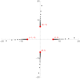
(a) $\Pi_{A}$

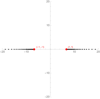
(b) $\Pi_{B}$

Figure 1: Poles of the Borel–Padé transforms, which would accumulate to branch cuts for the Borel transform of the quantum periods $\Pi_{A}(E,\hbar)$ (a) and $\Pi_{B}(E,\hbar)$ (b) at $u=0$ and $\Lambda=1$. The red points are the central charges of the BPS states which contribute to the branch points, and their electromagnetic charges are labelled nearby. See discussion in section 3.2.

Let us look at some examples of the Borel plane of the quantum periods for the modified Mathieu equation. In practice, to calculate the Borel transform, we use standard Borel–Padé techniques, i.e. we use a finite number of terms in the formal power series (in this case we have used $193$ terms), and in order to extend analytically the resulting function, we use a Padé transform of the Borel transform. In this method, branch cuts of the Borel transform are indicated by a dense accumulation of poles of the Borel–Padé transform along a segment. The first example is when $u=E=0$. We plot the poles of the Borel–Padé transforms of $\Pi_{A}(0,\hbar),\Pi_{B}(0,\hbar)$ in the Borel plane in Figures 1. They indicate the existence of four branch cuts in the case of the $A$ period, and two branch cuts in the case of $B$ period. Since in both cases there are branch cuts along the positive real axis, neither of the two quantum periods are Borel summable.

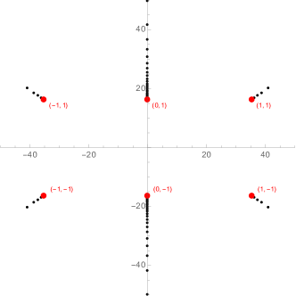
(a) $\Pi_{A}$

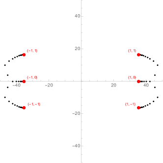
(b) $\Pi_{B}$

Figure 2: Poles of the Borel–Padé transforms, which would accumulate to branch cuts for the Borel transforms of the quantum periods $\Pi_{A}(u,\hbar)$ (a) and $\Pi_{B}(u,\hbar)$ (b) at $u=4$ and $\Lambda=1$. The red points are the central charges of the BPS states which contribute to the branch points, and their electromagnetic charges are labelled nearby. See discussion in section 3.2.

Next, we consider $u=E/2=4$. Again we plot the poles of the Borel–Padé transforms of $\Pi_{A}(4,\hbar),\Pi_{B}(4,\hbar)$ in the Borel plane in Figures 2. In both cases we observe six branch cuts, and they are in different locations as compared to what we found at $u=0$. In this case, the quantum $A$ period is Borel summable, but the quantum $B$ period is not.

As we can see, in general, the quantum periods are not Borel summable, and their Borel transforms and resummations have a rich structure. Fortunately the connection with SW theory gives very powerful information on this structure, which we will explore in detail in the next section.

3 Quantum periods from TBA equations

In this section we study the TBA equations which control the analytic properties of the quantum periods of the modified Mathieu equation. We set $\Lambda=1$ throughout the section.

3.1 Review of the TBA equations of Gaiotto–Moore–Neitzke

The TBA equations we will obtain are conformal limits oper of the integral equations proposed by Gaiotto–Moore–Neitzke (GMN) in gmn to describe the hyperKähler metric on the Coulomb branch of ${\cal N}=2$ theories compactified on $\mathbb{R}^{3}\times{\mathbb{S}}^{1}_{R}$, where $R$ is the compactification radius. We will now review some basic aspects of these equations which will be useful in the following. The basic ingredients in these equations are the central charges of the ${\cal N}=2$ supersymmetric gauge theory

$$Z(\boldsymbol{u})=\left(\boldsymbol{a},\boldsymbol{a}_{D}\right),$$ (3.35)

where

$$\boldsymbol{a}_{D}={\partial F_{0}\over\partial\boldsymbol{a}}.$$ (3.36)

We define the period associated to a vector $\boldsymbol{\gamma}\in\Gamma$ in the lattice of electromagnetic charges as

$$Z_{\boldsymbol{\gamma}}=Z(\boldsymbol{u})\cdot{\boldsymbol{\gamma}}.$$ (3.37)

This is just a linear combination of $A$ periods and $B$ periods.

To such a central charge we associate a ray

$$\ell_{\boldsymbol{\gamma}}=\left\{\zeta:{Z_{\boldsymbol{\gamma}}(\boldsymbol{u})\over\zeta}\in\mathbb{R}_{-}\right\}.$$ (3.38)

The semiflat coordinate on the Coulomb branch is given by

$$\chi_{\boldsymbol{\gamma}}^{\rm sf}(\zeta)=\exp\left[\pi R\zeta^{-1}Z_{\boldsymbol{\gamma}}+{\rm i}\theta_{\boldsymbol{\gamma}}+\pi R\overline{\zeta}Z_{\boldsymbol{\gamma}}\right],$$ (3.39)

where $R$ is the compactification radius, and

$$\theta_{\boldsymbol{\gamma}}=\boldsymbol{\theta}\cdot{\boldsymbol{\gamma}}$$ (3.40)

is the angular coordinate on the fiber. The semiflat coordinate is the “uncorrected” or “classical” coordinate, and it is corrected by exponentially small effects in the large $R$ limit. These effects are encoded in a non-linear, TBA-like integral equation, which reads as

$$\chi_{\boldsymbol{\gamma}}(\zeta)=\chi_{\boldsymbol{\gamma}}^{\rm sf}(\zeta)\exp\left[-{1\over 2\pi{\rm i}}\sum_{\boldsymbol{\gamma}^{\prime}\in\Gamma}\Omega(\boldsymbol{\gamma}^{\prime};\boldsymbol{u})\langle\boldsymbol{\gamma},\boldsymbol{\gamma}^{\prime}\rangle{\cal I}_{\boldsymbol{\gamma}^{\prime}}(\zeta)\right],$$ (3.41)

where $\Omega(\gamma;u)$ is the number of BPS states with electromagnetic charge $\gamma$ at the point $u$ of the Coulomb branch, and

$${\cal I}_{\boldsymbol{\gamma}}=\int_{\ell_{\boldsymbol{\gamma}}}{{\rm d}\zeta^{\prime}\over\zeta^{\prime}}{\zeta^{\prime}+\zeta\over\zeta^{\prime}-\zeta}\log\left(1-\sigma(\boldsymbol{\gamma})\chi_{\boldsymbol{\gamma}}(\zeta^{\prime})\right).$$ (3.42)

Here, $\sigma(\boldsymbol{\gamma})$ is the quadratic refinement. It has been argued in gmn2 that, for BPS hypermultiplets/vectormultiplets, one has, respectively,

$$\sigma(\boldsymbol{\gamma})=\mp 1.$$ (3.43)

We have used the normalization of cdorey , which is more appropriate for our normalization of charges/periods. An important feature of (3.41) is that only those states whose charge $\boldsymbol{\gamma^{\prime}}$ has a non-vanishing Dirac pairing with $\boldsymbol{\gamma}$ contributes to the equation of $\chi_{\boldsymbol{\gamma}}(\zeta)$. The quantities $\chi_{\boldsymbol{\gamma}}(\zeta)$ characterize in a precise way the hyperKähler metric of the moduli space of the ${\cal N}=2$ theory compactified on $\mathbb{R}^{3}\times{\mathbb{S}}^{1}_{R}$, and they can be realized as cluster coordinates on this moduli space gmn2 . They satisfy the property

$$\chi_{\boldsymbol{\gamma}+\boldsymbol{\gamma}^{\prime}}(\zeta)=\chi_{\boldsymbol{\gamma}}(\zeta)\chi_{\boldsymbol{\gamma}^{\prime}}(\zeta).$$ (3.44)

Very often we have both charges $\pm\boldsymbol{\gamma}$ appearing in the sum in the r.h.s. of (3.41). If $\theta_{\boldsymbol{\gamma}}=0$, we have an extra symmetry oper ,

$$\chi_{\boldsymbol{\gamma}}(\zeta)=\chi_{-\boldsymbol{\gamma}}(-\zeta),$$ (3.45)

and we can combine

$${\cal C}_{\boldsymbol{\gamma}}={\cal I}_{\boldsymbol{\gamma}}-{\cal I}_{-\boldsymbol{\gamma}} =\int_{\ell_{\boldsymbol{\gamma}}}{{\rm d}\zeta^{\prime}\over\zeta^{\prime}}{\zeta^{\prime}+\zeta\over\zeta^{\prime}-\zeta}\log\left(1-\sigma(\boldsymbol{\gamma})\chi_{\boldsymbol{\gamma}}(\zeta^{\prime})\right)-\int_{\ell_{-\boldsymbol{\gamma}}}{{\rm d}\zeta^{\prime}\over\zeta^{\prime}}{\zeta^{\prime}+\zeta\over\zeta^{\prime}-\zeta}\log\left(1-\sigma(-\boldsymbol{\gamma})\chi_{-\boldsymbol{\gamma}}(\zeta^{\prime})\right)$$ (3.46)

$$=\int_{\ell_{\boldsymbol{\gamma}}}{{\rm d}\zeta^{\prime}\over\zeta^{\prime}}\left({\zeta^{\prime}+\zeta\over\zeta^{\prime}-\zeta}-{\zeta^{\prime}-\zeta\over\zeta^{\prime}+\zeta}\right)\log\left(1-\sigma(\boldsymbol{\gamma})\chi_{\boldsymbol{\gamma}}(\zeta^{\prime})\right)$$

$$=4\zeta\int_{\ell_{\boldsymbol{\gamma}}}{{\rm d}\zeta^{\prime}\over\left(\zeta^{\prime}\right)^{2}-\zeta^{2}}\log\left(1-\sigma(\boldsymbol{\gamma})\chi_{\boldsymbol{\gamma}}(\zeta^{\prime})\right).$$

In going from the first to the second line we have changed variables $\zeta^{\prime}\rightarrow-\zeta^{\prime}$, and we used the symmetry (3.45).

In order to put the equations in a form similar to the TBA equations, we will perform a change of variables akin to the one made in gmn . If

$$Z_{\boldsymbol{\gamma}}={\rm e}^{{\rm i}\phi^{\prime}}\left|Z_{\boldsymbol{\gamma}}\right|$$ (3.47)

then we change variables in (3.46) as follows:

$$\zeta=-{\rm e}^{{\rm i}\phi-\theta},\qquad\zeta^{\prime}=-{\rm e}^{{\rm i}\phi^{\prime}-\theta^{\prime}},$$ (3.48)

and we obtain

$${\cal C}_{\boldsymbol{\gamma}}=2\int_{\mathbb{R}}{\log\left(1-\sigma(\boldsymbol{\gamma})\chi_{\boldsymbol{\gamma}}(\theta^{\prime})\right)\over\sinh(\theta-\theta^{\prime}+{\rm i}\phi^{\prime}-{\rm i}\phi)}{\rm d}\theta^{\prime}.$$ (3.49)

3.2 TBA equations for the modified Mathieu equation

Building on oper ; ims , we expect to have a general correspondence between the mathematical description of BPS states in gmn ; gmn2 , and the “resurgent” properties of the quantum periods associated to the corresponding SW curve. As noted in oper , this correspondence involves the conformal limit of the TBA equations of gmn , which is given by

$$R\to 0\ ,\quad\zeta\to 0\ ,\quad\zeta/R\;\;\text{finite}\ .$$ (3.50)

In this correspondence, the classical limit of the WKB periods $\Pi_{\gamma}^{(0)}$ corresponds to the central charge $Z_{\gamma}$, while the full quantum period is obtained as the logarithm of the Coulomb branch coordinates $\chi_{\gamma}(\zeta)$ (in the conformal limit). The Borel singularities of the Borel transforms $\widehat{\Pi}_{\gamma}$ are closely related to the BPS spectrum of the theory, and the Stokes discontinuities of the quantum periods are closely related to the so-called Kontsevich–Soibelman symplectomorphisms ks ; gmn ; gmn2 . This correspondence is summarized in Table 1, and it can be used to obtain integral equations of the TBA type governing the quantum periods. We will now apply this correspondence to obtain such equations for the modified Mathieu operator.

Resurgence	BPS states
WKB curve	SW curve
classical limit $\Pi_{\gamma}^{(0)}$	central charge $Z(\gamma)$
quantum period $\Pi_{\gamma}$	cluster coordinate $\log\,\chi_{\gamma}$
Borel singularities	BPS spectrum
Stokes discontinuities	KS symplectomorphisms

Table 1: Correspondence between the mathematical structures in the resurgent approach to the WKB method, and those in the theory of BPS states.

Let us then consider the SW theory sw , i.e. pure ${\cal N}=2$ SYM with gauge group $SU(2)$. We will denote the charge by

$$\boldsymbol{\gamma}=\gamma=(n_{e},n_{m}).$$ (3.51)

We will use the conventions of cdorey for the symplectic product,

$$\langle\gamma,\gamma^{\prime}\rangle=\langle(n_{e},n_{m}),(n^{\prime}_{e},n^{\prime}_{m})\rangle=-n_{e}n_{m}^{\prime}+n_{m}n^{\prime}_{e}.$$ (3.52)

We will denote

$$\chi_{e}(\zeta)=\chi_{(1,0)}(\zeta),\qquad\chi_{m}(\zeta)=\chi_{(0,1)}(\zeta),\qquad\chi_{d}(\zeta)=\chi_{(1,1)}(\zeta),$$ (3.53)

and because of (3.44) we have

$$\chi_{d}(\zeta)=\chi_{e}(\zeta)\chi_{m}(\zeta).$$ (3.54)

We will write TBA equations for $\chi_{e}(\zeta)$ and $\chi_{m}(\zeta)$, as in cdorey . We have

$$\chi_{e}(\zeta) =\chi^{\rm sf}_{e}(\zeta)\exp\left[-{1\over 2\pi{\rm i}}\sum_{\gamma^{\prime}}c_{e}(\gamma^{\prime}){\cal I}_{\gamma^{\prime}}(\zeta)\right],$$ (3.55)

$$\chi_{m}(\zeta) =\chi^{\rm sf}_{m}(\zeta)\exp\left[-{1\over 2\pi{\rm i}}\sum_{\gamma^{\prime}}c_{m}(\gamma^{\prime}){\cal I}_{\gamma^{\prime}}(\zeta)\right],$$

where

$$c_{e}(\gamma)=\Omega(\gamma;u)\langle(1,0),\gamma\rangle,\qquad c_{m}(\gamma)=\Omega(\gamma;u)\langle(0,1),\gamma\rangle.$$ (3.56)

In order to write the integral equations, we need to know the structure of the BPS spectrum in SW theory. It is known that there is a curve of marginal stability ${\cal C}$ in the Coulomb branch of the SW theory, separating a strong coupling region or chamber ${\cal S}$ inside ${\cal C}$, from a weak coupling region or chamber ${\cal W}$ outside ${\cal C}$ sw ; fb ; selfdual . As we move from the strong coupling region to the weak coupling region, the spectrum of BPS states changes drastically by the famous wall-crossing phenomenon. We consider the two chambers in turn.

3.2.1 Strong coupling region

We start with the region ${\cal W}$ inside the curve of marginal stability. The spectrum consists of one monopole with charge

$$\gamma_{m}=(0,1)$$ (3.57)

and one dyon with charge

$$\gamma_{d}=(1,1),$$ (3.58)

see sw ; fb ; selfdual (we follow the conventions in fb ). We also have the corresponding antiparticles, carrying opposite charges. Then, the only nonzero coefficients in (3.55) are

$$c_{e}(\gamma_{m})=c_{e}(\gamma_{d})=-1,\qquad c_{m}(\gamma_{d})=1.$$ (3.59)

Therefore, the equations (3.55) read

$$\chi_{e}(\zeta) =\chi^{\rm sf}_{e}(\zeta)\exp\left[{1\over 2\pi{\rm i}}\left({\cal C}_{\gamma_{m}}+{\cal C}_{\gamma_{d}}\right)\right],$$ (3.60)

$$\chi_{m}(\zeta) =\chi^{\rm sf}_{m}(\zeta)\exp\left[-{1\over 2\pi{\rm i}}{\cal C}_{\gamma_{d}}\right],$$

and it is better to write them in terms of $\chi_{d}$, $\chi_{m}$,

$$\chi_{d}(\zeta) =\chi^{\rm sf}_{d}(\zeta)\exp\left[{1\over 2\pi{\rm i}}{\cal C}_{\gamma_{m}}\right],$$ (3.61)

$$\chi_{m}(\zeta) =\chi^{\rm sf}_{m}(\zeta)\exp\left[-{1\over 2\pi{\rm i}}{\cal C}_{\gamma_{d}}\right].$$

We now write the central charges

$$Z_{d}={\rm e}^{{\rm i}\phi_{d}}|Z_{d}|,\qquad Z_{m}=-{\rm i}{\rm e}^{{\rm i}\phi_{m}}|Z_{m}|.$$ (3.62)

These conventions are such that, when $u\in\mathbb{R}$ inside the curve of marginal stability, we have $\phi_{d}=\phi_{m}=0$. Let us define the functions $\epsilon_{d,m}$ and $\widetilde{\epsilon}_{d,m}(\theta)$ as follows (this is similar to the notation used in amsv ; ims ):

$$\chi_{d}\left(-{\rm e}^{{\rm i}\phi_{d}-\theta}\right) =\exp\left(-\epsilon_{d}(\theta-{\rm i}\phi_{d})\right)=\exp\left(-\widetilde{\epsilon}_{d}(\theta)\right),$$ (3.63)

$$\chi_{m}\left({\rm i}{\rm e}^{{\rm i}\phi_{m}-\theta}\right) =\exp\left(-\epsilon_{m}(\theta-{\rm i}\phi_{m})\right)=\exp\left(-\widetilde{\epsilon}_{m}(\theta)\right).$$

Then, the conformal limit of the TBA equations reads:

$$\widetilde{\epsilon}_{d}(\theta) =\pi|Z_{d}|{\rm e}^{\theta}-2\int_{\mathbb{R}}{\widetilde{L}_{m}(\theta^{\prime})\over\cosh(\theta-\theta^{\prime}+{\rm i}\phi_{m}-{\rm i}\phi_{d})}{{\rm d}\theta^{\prime}\over 2\pi},$$ (3.64)

$$\widetilde{\epsilon}_{m}(\theta) =\pi|Z_{m}|{\rm e}^{\theta}-2\int_{\mathbb{R}}{\widetilde{L}_{d}(\theta^{\prime})\over\cosh(\theta-\theta^{\prime}+{\rm i}\phi_{d}-{\rm i}\phi_{m})}{{\rm d}\theta^{\prime}\over 2\pi},$$

where we have shifted $\theta\to\theta-\log R$, and

$$\widetilde{L}_{m,d}(\theta)=\log\left(1+{\rm e}^{-\widetilde{\epsilon}_{m,d}(\theta)}\right).$$ (3.65)

We have used here the fact that the BPS spectrum consists of hypermultiplets, therefore $\sigma(\gamma)=-1$.

The equations simplify further when $u$ is real, i.e. $u\in\mathbb{R}\cap{\cal W}=[-1,1]$. Then one has $\phi_{d}=\phi_{m}=0$, i.e.

$$Z_{\gamma_{d}}>0,\qquad Z_{\gamma_{m}}=-{\rm i}|Z_{\gamma_{m}}|,$$ (3.66)

and we obtain,

$$\epsilon_{d}(\theta) =\pi|Z_{d}|{\rm e}^{\theta}-2\int_{\mathbb{R}}{L_{m}(\theta^{\prime})\over\cosh(\theta-\theta^{\prime})}{{\rm d}\theta^{\prime}\over 2\pi},$$ (3.67)

$$\epsilon_{m}(\theta) =\pi|Z_{m}|{\rm e}^{\theta}-2\int_{\mathbb{R}}{L_{d}(\theta^{\prime})\over\cosh(\theta-\theta^{\prime})}{{\rm d}\theta^{\prime}\over 2\pi}.$$

We also note that, before taking the conformal limit, we find the more conventional TBA equations

$$\epsilon_{d}(\theta) =\pi rZ_{d}\cosh(\theta)-2\int_{\mathbb{R}}{L_{m}(\theta^{\prime})\over\cosh(\theta-\theta^{\prime})}{{\rm d}\theta^{\prime}\over 2\pi},$$ (3.68)

$$\epsilon_{m}(\theta) =\pi r|Z_{m}|\cosh(\theta)-2\int_{\mathbb{R}}{L_{d}(\theta^{\prime})\over\cosh(\theta-\theta^{\prime})}{{\rm d}\theta^{\prime}\over 2\pi},$$

where

$$r=2R.$$ (3.69)

The definition of $r$ is such that we have the same conventions as in kl-mel-1 .

The TBA equations simplify greatly when $u=0$. In this case, we have that

$$|Z_{d}|=|Z_{m}|=\xi,$$ (3.70)

and that

$$\epsilon_{d}(\theta)=\epsilon_{m}(\theta)=\epsilon(\theta).$$ (3.71)

The two TBA equations collapse to one,

$$\epsilon(\theta)=\pi\xi{\rm e}^{\theta}-2\int_{\mathbb{R}}{L(\theta^{\prime})\over\cosh(\theta-\theta^{\prime})}{{\rm d}\theta^{\prime}\over 2\pi},$$ (3.72)

which coincides with the integral equation (B.251) associated to the modified Mathieu equation and the Sinh-Gordon model and studied by Zamolodchikov (the factor $\xi$ can be absorbed in a redefinition of the angle $\theta$). The equation (3.72) was written down in oper as governing the quantum periods at $u=0$.

We claim that the functions $\widetilde{\epsilon}_{d,m}(\theta)$ are identified with quantum periods as follows

$$\widetilde{\epsilon}_{d}(x+{\rm i}\phi_{d}) =\frac{1}{\hbar}s(\Pi_{D})(\hbar),$$ (3.73)

$$\widetilde{\epsilon}_{m}\left(x+{\rm i}\phi_{m}-\frac{{\rm i}\pi}{2}\right) =\frac{1}{\hbar}s(\Pi_{B})(\hbar),$$

with

$$\hbar=\pi^{-1}{\rm e}^{-x},\quad\Pi_{D}=\Pi_{A}+\Pi_{B}\ ,$$ (3.74)

where $\Pi_{D}$ denotes the dyonic quantum period. Then the TBA equations (3.64) are consistent with the leading order contribution by the classical periods in the small $\hbar$ expansion

$$s(\Pi_{D,B})(\hbar)=Z_{d,m}+\mathcal{O}(\hbar^{2})\ .$$ (3.75)

Furthermore, the TBA equations (3.64) clearly indicate that for some argument angles of $\hbar$ the quantum periods have discontinuities. These discontinuities are determined by the BPS spectrum of SW theory and give the singularity structure of the Borel transform of the quantum periods. These Stokes discontinuities can also be deduced from (3.64). The location of the singularities in the Borel plane, as well as the precise discontinuities, can be checked against the asymptotic series of the quantum periods, by inspecting the Borel plane and by performing lateral Borel resummations, respectively.

For instance, from the TBA equations (3.64), we conclude that $s(\Pi_{B})$ are discontinuous across the rays $\arg(\hbar)=\phi_{d},\phi_{d}+\pi$, with

$$\text{disc}_{\phi_{d}(+\pi)}(\Pi_{B})(\hbar)= +2\hbar\log\left(1+{\rm e}^{-\tfrac{1}{\hbar}s(\Pi_{D})(\hbar)}\right)$$

$$= 2\hbar\left({\rm e}^{-\tfrac{1}{\hbar}s(\Pi_{D})(\hbar)}-\frac{1}{2}{\rm e}^{-2\tfrac{1}{\hbar}s(\Pi_{D})(\hbar)}+\ldots\right)\ .$$ (3.76)

When $u=0$, we have $\phi_{d}=0$, and the discontinuities are located at $\arg(\hbar)=0,\pi$. The discontinuity across the ray $\arg(\hbar)=0$ can be computed by a lateral Borel resummation of the quantum $B$ period. We check it against the right hand side of (3.76), and find good agreement. See Table 2. Similarly, $s(\Pi_{D})$ is discontinuous across the rays $\arg(\hbar)=\phi_{m}\pm\frac{\pi}{2}$, and one has

$$\text{disc}_{\phi_{m}\pm\frac{\pi}{2}}(\Pi_{D})(\hbar)=-2\hbar\log\left(1+{\rm e}^{-\tfrac{1}{\hbar}s(\Pi_{B})(\hbar)}\right)\ .$$ (3.77)

Numerical checks for this discontinuity formula are completely analogous.

terms	lateral Borel sum	r.h.s. of (3.76)
181	0.17499253901611	0.1749925390148815032360
185	0.17499253901578	0.1749925390148815032482
189	0.17499253901545	0.1749925390148815032553
193	0.17499253901519	0.1749925390148815032595

Table 2: Discontinuity across the ray $\arg(\hbar)=0$ for $\Pi_{B}(u=0,\hbar=1)$ computed by lateral Borel resummation and by using (3.76) with increasing number of terms in the asymptotic series. Underlined are stabilised digits.

From the discontinuity formula (3.76) we can deduce in the standard way a formula for the large order behavior of $\Pi_{B}^{(n)}$, of the form (see e.g. msw )

$${\rm i}\Pi_{B}^{(n)}\sim\frac{2A^{-2n+b}}{\pi}\Gamma(2n+b)$$

$$\cdot\left(1-\frac{\mu_{2}A}{2n+b-1}+\frac{\mu_{3}A^{2}}{(2n+b-1)(2n+b-2)}-\frac{\mu_{4}A^{3}}{(2n+b-1)(2n+b-2)(2n+b-3)}\cdots\right).$$ (3.78)

If we write the dyonic quantum period as

$$\Pi_{D}=\sum_{n\geq 0}\Pi_{D}^{(n)}\hbar^{2n},$$ (3.79)

we can identify

$$A=\Pi_{D}^{(0)},\quad b=-1,\quad\mu_{2}=\Pi_{D}^{(1)},\quad\mu_{3}=(\Pi_{D}^{(1)})^{2}/2,\quad\mu_{4}=(\Pi_{D}^{(1)})^{3}/6+\Pi_{D}^{(2)},\quad\ldots$$ (3.80)

These identities are numerically checked at $u=0$ up to all stabilised digits (more than 40) with the help of Richardson transforms.

The large order behavior of $\Pi_{B}^{(n)}$ also indicates that the Borel transform $\widehat{\Pi}_{B}(\zeta)$ has branch points at $\zeta=\pm\Pi_{D}^{(0)}$, which is the central charge of the BPS state (dyon) whose electromagnetic charge has non-vanishing Dirac pairing with the charge of the monopole. Similarly, the Borel transform of $\Pi_{A}(u,\hbar)$ should have branch points at the central charges of monopoles and dyons with electromagnetic charges $\pm(0,1),\pm(1,1)$, while the Borel transform of $\Pi_{B}(u,\hbar)$ have branch points only at the central charges of dyons. This explains the Borel plane plots in Figure 1, where we also superimpose the central charges of the contributing BPS states as red spots.

3.2.2 Weak coupling region

Let us now consider the region outside the curve of marginal stability. The spectrum consists of dyons with charge $\pm\gamma_{n}$, where

$$\gamma_{n}=(n,1),\qquad n\in\mathbb{Z},$$ (3.81)

and $W$ boson with charges $\pm\gamma_{e}$, where

$$\gamma_{e}=(1,0).$$ (3.82)

From (3.56) we conclude that

$$c_{e}(\gamma_{n})=-1$$ (3.83)

and

$$c_{m}(\gamma_{n})=n,\qquad c_{m}(\gamma_{e})=2,$$ (3.84)

where we used the fact that

$$\Omega(\gamma_{e};u)=2$$ (3.85)

in the weak coupling region.

As in cdorey , we write the equations for $\chi_{e}$, $\chi_{m}$. We find

$$\chi_{m}(\zeta) =\chi_{m}^{\rm sf}(\zeta)\exp\left[-{1\over\pi{\rm i}}{\cal C}_{\gamma_{e}}(\zeta)-{1\over 2\pi{\rm i}}\sum_{n\in\mathbb{Z}}n{\cal C}_{\gamma_{n}}(\zeta)\right],$$ (3.86)

$$\chi_{e}(\zeta) =\chi_{e}^{\rm sf}(\zeta)\exp\left[{1\over 2\pi{\rm i}}\sum_{n\in\mathbb{Z}}{\cal C}_{\gamma_{n}}(\zeta)\right].$$

In this region we will write

$$Z_{m}={\rm i}{\rm e}^{{\rm i}\phi_{m}}|Z_{m}|,\qquad Z_{e}={\rm e}^{{\rm i}\phi_{e}}|Z_{e}|,\qquad Z_{\ell}={\rm e}^{{\rm i}\phi_{\ell}}|Z_{\ell}|,$$ (3.87)

where we have denoted $Z_{\ell}=Z_{\gamma_{\ell}}$ the central charge of a dyon. This is chosen in such a way that, if $u$ is real, we have $\phi_{e}=\phi_{m}=0$. We now define

$$\chi_{e}\left(-{\rm e}^{{\rm i}\phi_{e}-\theta}\right) =\exp\left(-\epsilon_{e}(\theta-{\rm i}\phi_{e})\right)=\exp\left(-\widetilde{\epsilon}_{e}(\theta)\right),$$ (3.88)

$$\chi_{m}\left(-{\rm i}\,{\rm e}^{{\rm i}\phi_{m}-\theta}\right) =\exp\left(-\epsilon_{m}(\theta-{\rm i}\phi_{m})\right)=\exp\left(-\widetilde{\epsilon}_{m}(\theta)\right),$$

$$\chi_{\ell}\left(-\,{\rm e}^{{\rm i}\phi_{\ell}-\theta}\right) =\exp\left(-\epsilon_{\ell}(\theta-{\rm i}\phi_{\ell})\right)=\exp\left(-\widetilde{\epsilon}_{\ell}(\theta)\right),$$

We then obtain the equations,

$$\widetilde{\epsilon}_{e}(\theta) =\pi|Z_{e}|{\rm e}^{\theta}+{1\over\pi}\int_{\mathbb{R}}{\widetilde{L}_{m}(\theta^{\prime})\over\cosh(\theta-\theta^{\prime}+{\rm i}\phi_{m}-{\rm i}\phi_{e})}{\rm d}\theta^{\prime}+{1\over\pi{\rm i}}\sum_{\ell\not=0}\int_{\mathbb{R}}{\widetilde{L}_{\ell}(\theta^{\prime}){\rm d}\theta^{\prime}\over\sinh(\theta-\theta^{\prime}+{\rm i}\phi_{\ell}-{\rm i}\phi_{e})},$$ (3.89)

$$\widetilde{\epsilon}_{m}(\theta) =\pi|Z_{m}|{\rm e}^{\theta}-{2\over\pi}\int_{\mathbb{R}}{\widetilde{L}_{e}(\theta^{\prime}){\rm d}\theta^{\prime}\over\cosh(\theta-\theta^{\prime}+{\rm i}\phi_{e}-{\rm i}\phi_{m})}-{1\over\pi}\sum_{\ell\in\mathbb{Z}}\ell\int_{\mathbb{R}}{\widetilde{L}_{\ell}(\theta^{\prime}){\rm d}\theta^{\prime}\over\cosh(\theta-\theta^{\prime}+{\rm i}\phi_{\ell}-{\rm i}\phi_{m})}$$

where

$$\widetilde{L}_{e,m}(\theta)=\log\left(1\mp{\rm e}^{-\widetilde{\epsilon}_{e,m}(\theta)}\right),\qquad\widetilde{L}_{\ell}(\theta)=\log\left(1+{\rm e}^{-\widetilde{\epsilon}_{\ell}(\theta)}\right).$$ (3.90)

Here we have assumed that

$$\sigma(\gamma_{e})=1,$$ (3.91)

since the $W$ boson is a vector multiplet gmn2 . In the equation for $\widetilde{\epsilon}_{e}(\theta)$ we have written down explicitly the term corresponding to the dyon with zero electric charge $\gamma_{\ell=0}=\gamma_{m}$, which is the magnetic monopole. We can also deduce the TBA equation for $\widetilde{\epsilon}_{\ell}(\theta)$, by combining the two equations above. We find

$$\widetilde{\epsilon}_{\ell}(\theta)=\pi|Z_{\ell}|{\rm e}^{\theta}+{2\over\pi{\rm i}}\int_{\mathbb{R}}{\widetilde{L}_{e}(\theta^{\prime}){\rm d}\theta^{\prime}\over\sinh(\theta-\theta^{\prime}+{\rm i}\phi_{e}-{\rm i}\phi_{\ell})}+{1\over\pi{\rm i}}\sum_{k\in\mathbb{Z}}(\ell-k)\int_{\mathbb{R}}{\widetilde{L}_{k}(\theta^{\prime}){\rm d}\theta^{\prime}\over\sinh(\theta-\theta^{\prime}+{\rm i}\phi_{k}-{\rm i}\phi_{\ell})}.$$ (3.92)

It is useful to isolate the contribution from the magnetic monopole $k=0$ explicitly in the last term, so that we obtain

$$\widetilde{\epsilon}_{\ell}(\theta) =\pi|Z_{\ell}|{\rm e}^{\theta}+{2\over\pi{\rm i}}\int_{\mathbb{R}}{\widetilde{L}_{e}(\theta^{\prime}){\rm d}\theta^{\prime}\over\sinh(\theta-\theta^{\prime}+{\rm i}\phi_{e}-{\rm i}\phi_{\ell})}+{1\over\pi{\rm i}}\sum_{k\not=0}(\ell-k)\int_{\mathbb{R}}{\widetilde{L}_{k}(\theta^{\prime}){\rm d}\theta^{\prime}\over\sinh(\theta-\theta^{\prime}+{\rm i}\phi_{k}-{\rm i}\phi_{\ell})}$$ (3.93)

$$-{\ell\over\pi}\int_{\mathbb{R}}{\widetilde{L}_{m}(\theta^{\prime}){\rm d}\theta^{\prime}\over\cosh(\theta-\theta^{\prime}+{\rm i}\phi_{m}-{\rm i}\phi_{\ell})}.$$

The above equations have some interesting reality properties along the real axis, where $\phi_{e}=\phi_{m}=0$. In that case, since

$$Z_{\ell}=\ell|Z_{e}|+{\rm i}|Z_{m}|,$$ (3.94)

one has that

$$\phi_{\ell}+\phi_{-\ell}=\pi,\qquad\ell\in\mathbb{Z}.$$ (3.95)

It is then easy to see that the conjugation property

$$\widetilde{\epsilon}_{-\ell}(\theta)=\widetilde{\epsilon}^{*}_{\ell}(\theta)$$ (3.96)

is compatible with the TBA system. In addition, $\epsilon_{e,m}(\theta)$ are real in this case.

In the weak coupling region, we propose the following identification with quantum periods

$$\widetilde{\epsilon}_{m}\left(x+{\rm i}\phi_{m}+\frac{{\rm i}\pi}{2}\right)= \frac{1}{\hbar}s(\Pi_{B})(\hbar),$$ (3.97)

$$\widetilde{\epsilon}_{e}(x+{\rm i}\phi_{e})= \frac{1}{\hbar}s(\Pi_{A})(\hbar),$$

$$\widetilde{\epsilon}_{\ell}(x+{\rm i}\phi_{\ell})= \frac{1}{\hbar}s(\Pi_{\ell})(\hbar),$$

with

$$\hbar=\pi^{-1}{\rm e}^{-x},\quad\Pi_{\ell}=\ell\Pi_{A}+\Pi_{B}\ .$$ (3.98)

The TBA equations (3.89) then imply that the Borel transforms of $\Pi_{A}(\hbar),\Pi_{B}(\hbar)$ have branch points at the central charges of the BPS states whose electromagnetic charges have non-vanishing Dirac pairing with those of the W-boson and monopole, respectively. For $\Pi_{A}(\hbar)$, these are the BPS states with charges $\pm(\ell,\pm 1),\ell=0,1,2,\ldots$; for $\Pi_{B}(\hbar)$, these are the BPS states with charges $\pm(1,0),\pm(\ell,\pm 1),\ell=1,2,\ldots$. This explains the Borel plane plots in Figure 2 with $u=4$, well in the weak coupling region. We also superimpose in the plots the central charges of the contributing BPS states as red spots.

In addition, the TBA equations (3.89) also indicate the following discontinuities for the resummed quantum periods $s(\Pi_{A})(\hbar)$, $s(\Pi_{B})(\hbar)$ in the $\hbar$-plane. The resummed quantum $A$ period $s(\Pi_{A})$ is discontinuous

• across the rays $\arg(\hbar)=\phi_{m}\pm\frac{\pi}{2}$ with the discontinuity

  $$\text{disc}_{\phi_{m}\pm\frac{\pi}{2}}(\Pi_{A})=-2\hbar\log(1+{\rm e}^{-\tfrac{1}{\hbar}s(\Pi_{B})(\hbar)})\ ;$$ (3.99)

• across the rays $\arg(\hbar)=\phi_{\ell}(+\pi)$ with the discontinuity

  $$\text{disc}_{\phi_{\ell}(+\pi)}(\Pi_{A})=2\hbar\log(1+{\rm e}^{-\tfrac{1}{\hbar}s(\Pi_{\ell})(\hbar)})\ ,\quad\ell\in\mathbb{Z}\ .$$ (3.100)

On the other hand, the quantum $B$ period $s(\Pi_{B})$ is discontinuous

• across the rays $\arg(\hbar)=\phi_{e}(+\pi)$ with the discontinuity

  $$\text{disc}_{\phi_{e}(+\pi)}(\Pi_{B})=-4\hbar\log(1-{\rm e}^{-\tfrac{1}{\hbar}s(\Pi_{A})(\hbar)})\ ;$$ (3.101)

• across the rays $\arg(\hbar)=\phi_{\ell}(+\pi)$ ($\ell\neq 0$) with the discontinuity

  $$\text{disc}_{\phi_{\ell}(+\pi)}(\Pi_{B})=-2\ell\hbar\log(1+{\rm e}^{-\tfrac{1}{\hbar}s(\Pi_{\ell})(\hbar)})\ ,\quad\ell\neq 0\ .$$ (3.102)

To test these formulae, we consider the case of $u=1+4{\rm i}$, where the branch cuts of the Borel transform of quantum $A$ and $B$ periods are well separated, as seen in Figure 3. We compute the discontinuity via lateral Borel resummation for various rays and find good agreement with the r.h.s. of the formulae (3.99)–(3.102), see Tables 3,4.

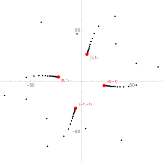
(a) $\Pi_{A}$

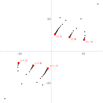
(b) $\Pi_{B}$

Figure 3: Poles of the Borel–Padé transforms, which would accumulate to branch cuts for the Borel transform of the quantum periods $\Pi_{A}(E,\hbar)$ (a) and $\Pi_{B}(E,\hbar)$ (b) at $u=1+4{\rm i}$ and $\Lambda=1$. The red points are the central charges of the BPS states which contribute to the branch points, and their electromagnetic charges are labelled nearby.

BPS state	$(0,-1)$	$(1,1)$
lateral Borel sum	$1.77819420225\times 10^{-10}-{\rm i}4.0146843089\times 10^{-11}$	$5.37838410\times 10^{-13}+{\rm i}3.166367886\times 10^{-12}$
r.h.s. of (3.99),(3.100)	$1.7781942022540\times 10^{-10}-{\rm i}4.014684308966\times 10^{-11}$	$5.3783841037\times 10^{-13}+{\rm i}3.16636788673\times 10^{-12}$

Table 3: Discontinuity of $\Pi_{A}(u=1+4{\rm i},\hbar=1)$ across the rays associated to BPS states $\gamma=(0,-1),(1,1)$, computed by lateral Borel resummation and by using (3.99),(3.100) with up to 193 terms in the asymptotic series. Only stabilised digits are listed.

BPS state	$(1,1)$	$(1,0)$
lateral Borel sum	$5.37838\times 10^{-13}+{\rm i}3.166367\times 10^{-12}$	$5.979\times 10^{-16}+{\rm i}4.701\times 10^{-16}$
r.h.s. of (3.101),(3.102)	$5.3783841\times 10^{-13}+{\rm i}3.16636788\times 10^{-12}$	$5.97982\times 10^{-16}+{\rm i}4.70119\times 10^{-16}$

Table 4: Discontinuity of $\Pi_{B}(u=1+4{\rm i},\hbar=1)$ across the rays associated to BPS states $\gamma=(1,1),(1,0)$, computed by lateral Borel resummation and by using (3.101),(3.102) with up to 193 terms in the asymptotic series. Only stabilised digits are listed.

Finally, we would like to mention that different TBA-like equations for the quantum periods of the modified Mathieu operator have been proposed in ito-shu-unp and more recently in h-neitzke .

3.3 Solving the TBA equations in the strong coupling region

As we have argued, Borel sums of quantum periods are solutions to the TBA equations (3.64),(3.89). In principle the resummed quantum periods can be computed from these TBA equations by using the dictionaries (3.73) and (3.97). In practice, however, these equations are difficult to use. First of all, one needs information on the boundary conditions at strong coupling in order to solve the equations. In addition, the standard tools to solve these equations numerically converge very slowly.

Let us first consider the simplest example at $u=0$, where the TBA system collapses to a single equation (3.72), which we reproduce here (we have absorbed the factor $\xi$ in (3.72) in the angle $\theta$)

$$\epsilon(\theta)=\pi{\rm e}^{\theta}-\int_{\mathbb{R}}\frac{\log(1+{\rm e}^{-\epsilon(\theta^{\prime})})}{\pi\cosh(\theta-\theta^{\prime})}{\rm d}\theta^{\prime}\,.$$ (3.103)

The solution can be identified with the quantum dyon period through the dictionary

$$\epsilon(\theta)=\frac{1}{\hbar}s(\Pi_{D})(u=0,\hbar)\ ,\quad\hbar=\Pi^{(0)}_{D}\pi^{-1}{\rm e}^{-\theta}={16\sqrt{\pi}\over\Gamma\left({1\over 4}\right)^{2}}{\rm e}^{-\theta}\ .$$ (3.104)

Furthermore, the asymptotic behavior of the solution $\epsilon(\theta)$ as $\theta\rightarrow\infty$ is of the form

$$\epsilon(\theta)\sim\pi{\rm e}^{\theta}+\sum_{n\geq 1}\epsilon^{(n)}{\rm e}^{(1-2n)\theta},$$ (3.105)

whose coefficients are identified with the quantum corrections to the dyon period

$$\epsilon^{(n)}=\frac{1}{\pi^{2n-1}}(\Pi^{(0)}_{D})^{2n-1}\Pi_{D}^{(n)}\ .$$ (3.106)

It turns out that the equation (3.103) admits many possible boundary conditions at $\theta\rightarrow-\infty$. This is in stark contrast to the TBA equations for polynomial potentials studied in oper ; ims , where the equations themselves fix the behavior of the solutions at $\theta\rightarrow-\infty$. One possibility for the boundary conditions at $\theta\rightarrow-\infty$ is the linear behavior (5.196). This type of behavior was considered by Zamolodchikov in post-zamo but in a slightly different context, as we will discuss in Sec. 5 (see also Appendix B). However, it can be seen that this is not well suited for the quantum periods we are studying. One quick way to see this is that the linear boundary condition with $P\not=0$ implies $\epsilon^{(1)}<-1/3$ (c.f. (B.261)), while from the quantum Matone relation (2.27) we find

$$\epsilon^{(1)}=\frac{1}{\pi}\Pi_{D}^{(0)}\Pi_{D}^{(1)}=\frac{1}{2\pi{\rm i}}\left(\Pi_{A}^{(0)}\Pi_{B}^{(1)}-\Pi_{B}^{(0)}\Pi_{A}^{(1)}\right)=-\frac{1}{3}.$$ (3.107)

It turns out that the appropriate boundary condition in this case is given by

$$\epsilon(\theta)=-2\log\left(-{2\theta\over\pi}\right)+\cdots,\qquad\theta\to-\infty\ .$$ (3.108)

This boundary condition for the TBA equation (3.103) was also studied by Zamolodchikov in zamo-reso . One can use a small modification of the “dilogarithm trick” of zamo-TBA to show that, with the boundary condition (3.108), one has indeed (3.107) (in the context of zamo-reso , this calculation gives the central charge $c=1$ for the corresponding sinh-Gordon theory).

To implement numerically the boundary condition (3.108), we borrow a trick from post-zamo . We define a continuous function

$$f_{1}(\theta)=-2\log\left(1+\frac{2}{\pi}\log(1+{\rm e}^{-\theta})\right),$$ (3.109)

which has the same boundary behavior as (3.108) and is exponentially suppressed when $\theta\to+\infty$. We then look for a function $F_{1}(\theta)$ which satisfies

$$f_{1}(\theta)=\int_{\mathbb{R}}K(\theta-\theta^{\prime})F_{1}(\theta^{\prime}){\rm d}\theta^{\prime}\ ,\quad K(\theta)=\frac{1}{\pi\cosh(\theta)}\ .$$ (3.110)

The generic solution to this linear integral equation is

$$F_{1}(\theta)=\frac{1}{2}\left(f_{1}\left(\theta+{\rm i}\frac{\pi}{2}\right)+f_{1}\left(\theta-{\rm i}\frac{\pi}{2}\right)\right)\ .$$ (3.111)

For our particular $f_{1}(\theta)$, we thus have

$$F_{1}(\theta)=-\log\left(1+\frac{2}{\pi}\log(1+{\rm i}{\rm e}^{-\theta})\right)-\log\left(1+\frac{2}{\pi}\log(1-{\rm i}{\rm e}^{-\theta})\right)\ .$$ (3.112)

This is a real function for $\theta\in\mathbb{R}$. The TBA equation (3.103) can then be written as

$$\epsilon(\theta)=\pi{\rm e}^{\theta}+f_{1}(\theta)-\int_{\mathbb{R}}{\rm d}\theta^{\prime}\frac{1}{\pi\cosh(\theta-\theta^{\prime})}\left(\log(1+{\rm e}^{-\epsilon(\theta^{\prime})})+F_{1}(\theta^{\prime})\right)\ ,$$ (3.113)

where both boundary conditions at $\pm\infty$ are explicitly spelt out.

The numerical solution to the TBA equation (3.103) converges rather slowly, and we managed to obtain 6 stabilised digits for $\hbar=1$ and 7 stabilised digits for $\hbar=1/2$. These results, on the other hand, do agree with the Borel resummation of the quantum dyon period. See Table 5.

	$\hbar=1$	$\hbar=1/2$
TBA	6.62781	13.47880
Borel sum	6.62781917$\ldots$	13.47880936$\ldots$

Table 5: Quantum dyon period at $u=0$.

Let us now move away from the point $u=0$ but remain in the strong coupling region with $u\in(-1,0)\cup(0,1)$. The TBA system (3.67) has two integral equations coupled to each other. Nevertheless, at $\theta\to-\infty$ the first terms $\propto{\rm e}^{\theta}$ on the r.h.s. of both equations in (3.67) are negligible, and the TBA system also collapses to the single equation (3.103) (with the first term on the r.h.s. suppressed). Therefore both $\epsilon_{d}(\theta),\epsilon_{m}(\theta)$ should have the same boundary condition as (3.108), in other words

$$\epsilon_{d}(\theta)\sim\epsilon_{m}(\theta)\sim-2\log\left(-\frac{2\theta}{\pi}\right)+\ldots\ ,\quad\theta\to-\infty\ .$$ (3.114)

This is corroborated by the fact that the Matone relation (3.107) can be reproduced with this boundary behavior by using again a slight modification of the “dilogarithm trick” zamo-TBA . We use again the trick of inserting the pair of $f_{1}(\theta),F_{1}(\theta^{\prime})$ functions, and we find that the numerical solution to the TBA system (3.67) has roughly the same speed of convergence as the solution to (3.103) for $u=0$. We tabulate the results for $u=1/3$ in Tables 6,7 and they also agree with the Borel sum of the quantum periods. Note that the TBA system is solved with $\theta\in\mathbb{R}$, which in light of (3.73) corresponds to real $\hbar$ for the quantum dyon period and to imaginary $\hbar$ for the quantum monopole period.

	$\hbar=1$	$\hbar=1/2$
TBA	$9.16476$	$18.61486$
Borel sum	$9.16476545\ldots$	$18.61486738\ldots$

Table 6: Quantum dyon period at $u=1/3$.

	$\hbar=-{\rm i}$	$\hbar=-{\rm i}/2$
TBA	$4.26480$	$8.716486$
Borel sum	$4.26480153\ldots$	$8.716486917\ldots$

Table 7: Quantum monopole period at $u=1/3$.

4 Quantum periods from instanton calculus

Instanton calculus n ; ns leads to a resummation of the quantum periods of the modified Mathieu equation (2.22), as pointed out in mirmor . This produces exact functions of $\hbar$ which we will denote by

$$\Pi_{A,B}^{\rm ex}(E,\hbar).$$ (4.115)

In this section we explain this resummation in detail and we compare it to the Borel resummation obtained in the context of the exact WKB method.

4.1 Review of instanton calculus

Let us first review some basic ingredients of instanton calculus in the 4d $N=2$ SYM with gauge group $G=SU(N)$ n ; no2 ; ns ; Flume:2002az ; bfmt .

We denote a partition (or Young tableaux) by

$$Y=(y_{1},y_{2},\cdots),$$ (4.116)

its transposed by

$$Y^{t}=(y_{1}^{t},y_{2}^{t},\cdots),$$ (4.117)

and a vector of Young tableaux as

$$\boldsymbol{Y}=(Y_{1},\cdots,Y_{N}).$$ (4.118)

It is useful to define

$$h_{Y}(s)=y_{i}-j,\qquad v_{Y}(s)=y^{t}_{j}-i,$$ (4.119)

where $s=(i,j)$ is a box (not necessarily in the partition $Y$). We will also use

$$\ell(\boldsymbol{Y})=\sum_{I=1}^{N}\ell(Y_{I})\ ,$$ (4.120)

whith

$$\ell(Y)=\sum_{i}y_{i}\ .$$ (4.121)

The four dimensional $SU(N)$ Nekrasov partition function is n ; Flume:2002az

$$Z(\boldsymbol{a};\epsilon_{1},\epsilon_{2})=\sum_{\boldsymbol{Y}}\left((-1)^{N}\Lambda^{2N}\right)^{\ell(\boldsymbol{Y})}{\cal Z}_{\boldsymbol{Y}},$$ (4.122)

where

$${\cal Z}_{\boldsymbol{Y}} =\prod_{I,J=1}^{N}\prod_{s\in Y_{I}}{1\over\alpha_{I}-\alpha_{J}-\epsilon_{1}v_{Y_{J}}(s)+\epsilon_{2}\left(h_{Y_{I}}(s)+1\right)}$$ (4.123)

$$\qquad\qquad\times\prod_{s\in Y_{J}}{1\over\alpha_{I}-\alpha_{J}+\epsilon_{1}\left(v_{Y_{I}}(s)+1\right){-}\epsilon_{2}h_{Y_{J}}(s)},$$

with

$$\sum_{i=1}^{N}\alpha_{i}=0,$$ (4.124)

and

$$a_{i}=\alpha_{i}-\alpha_{i+1},\quad i=1,\cdots,N-1.$$ (4.125)

The four dimensional $SU(N)$ Nekrasov-Shatashvili (NS) free energy is then defined by ns

$$F_{\rm NS}^{\rm inst}(\boldsymbol{a},\hbar)={\rm i}\hbar\,\lim_{\epsilon_{2}\rightarrow 0}\,\epsilon_{2}\log Z(\boldsymbol{a};{\rm i}\hbar,\epsilon_{2}).$$ (4.126)

An important property of this free energy is that it is given as a power series in $\Lambda$ which is expected to have a non-vanishing radius of convergence in a certain range of values of $a$ and $\hbar$ around the semiclassical region $|\Lambda/a|\ll 1$.

In order to make contact with the (modified) Mathieu equation, the relevant gauge theory is ${\cal N}=2$, $SU(2)$ SYM theory, hence we have to consider (4.126) with $N=2$. In this case the first few terms read

$$F_{\rm NS}^{\rm inst}(a,\hbar)=-\frac{2\Lambda^{4}}{a^{2}+\hbar^{2}}+\frac{\Lambda^{8}\left(7\hbar^{2}-5a^{2}\right)}{\left(a^{2}+\hbar^{2}\right)^{3}\left(a^{2}+4\hbar^{2}\right)}+{\cal O}\left(\Lambda^{16}\right).$$ (4.127)

Once the NS free energy is known, the quantum $A$ period $a(u,\hbar)$ can be obtained by inverting the quantum Matone relation acdkv ; lmn ; francisco ; bk ; bkk ; fm-wilson ; sciarappa1

$$u={a^{2}\over 8}-{\Lambda\over 8}\partial_{\Lambda}F_{\rm NS}^{\rm inst}(a,\hbar,\Lambda).$$ (4.128)

This leads to a series expansion for $a(u,\hbar)$ in powers of $\Lambda^{4}$ which is expected to converge in an appropriate range of the parameters $\Lambda$, $E$, $\hbar$ around the semiclassical region $|\Lambda^{2}/E|\ll 1$. The quantum $B$ period $a_{D}(u,\hbar)$ is then obtained from the quantum special geometry relation

$$a_{D}(a,\hbar)=\partial_{a}F_{\rm NS}(a,\hbar,\Lambda)= 2\gamma(a,\hbar,\Lambda)+\partial_{a}F_{\rm NS}^{\rm inst}(a,\hbar,\Lambda)$$ (4.129)

where hm

$$\gamma(a,\hbar)=\frac{a}{2}\log\left({\hbar^{2}\over\Lambda^{2}}\right)-\frac{\pi\hbar}{4}-\frac{{\rm i}\hbar}{2}\left(\log\Gamma\left(1+\frac{{\rm i}a}{\hbar}\right)-\log\Gamma\left(1-\frac{{\rm i}a}{\hbar}\right)\right)\ ,$$ (4.130)

and we replace $a$ by $a(u,\hbar)$.

We also note that it is possible to express the NS free energy via a TBA system ns ; kt2 (different from the one discussed in section 3.2). This TBA system however has a range of validity/convergence which is smaller than the one of the instanton calculus. For instance, the TBA breaks down if ${\rm Re}(a)\neq 0$, while the instanton counting expression for $F_{\rm NS}^{\rm inst}$ (4.126) is still well defined.

It was found in mirmor that by expanding (4.127), (4.128) at small values of $\hbar$, it is possible to recover the WKB periods (2.22). More precisely, at order $\hbar^{2n}$, one finds an expansion in $\Lambda$ which agrees with the expansion of $\Pi^{(n)}(E)$ at large $E$:

$$2\pi\,a(u,\hbar)\longrightarrow\sum_{n=0}^{\infty}\hbar^{2n}\Pi_{A}^{(n)}(E=2u),$$ (4.131)

$$2{\rm i}\,a_{D}(a(u,\hbar),\hbar)=2{\rm i}\partial_{a}(F_{\rm NS}(a,\hbar))\Big{|}_{a=a(u,\hbar)}\longrightarrow\sum_{n=0}^{\infty}\hbar^{2n}\Pi_{B}^{(n)}(E=2u).$$

Therefore, the Bethe/gauge correspondence provides an analytic way to resum the WKB periods period into well defined functions which are exact in $\hbar$. We will denote these functions by $\Pi_{A,B}^{\rm ex}(E,\hbar)$, and we will refer to them as “exact” quantum periods. In terms of the quantities that we have introduced, they are given by

$$\Pi^{\rm ex}_{A}(E,\hbar) =2\pi a(E,\hbar),$$ (4.132)

$$\Pi_{B}^{\rm ex}(E,\hbar) ={2{\rm i}}\partial_{a}F_{\rm NS}(a(E,\hbar),\hbar),$$

where we use the notation $a(E,\hbar):=a(u=E/2,\hbar)$.

It turns out that one can find the series expansion for $a(u,\hbar)$ by using elementary methods. To do this, we use the WKB method, but we solve the Riccati equation (2.3) perturbatively in $\Lambda$, i.e. we solve

$$Y^{2}(x)-{\rm i}\hbar\frac{{\rm d}Y(x)}{{\rm d}x}=E-2\Lambda^{2}\cosh(x)$$ (4.133)

with an ansatz

$$Y(x)=\sum_{n\geq 0}Y_{n}(x,\hbar,E)\Lambda^{2n}.$$ (4.134)

Clearly, we should set

$$Y_{0}(x,\hbar,E)={\sqrt{E}},$$ (4.135)

The equation for $Y_{1}(x,\hbar,E)$ is

$$2Y_{0}Y_{1}-{{\rm i}\hbar}{{\rm d}Y_{1}\over{\rm d}x}=-2\cosh(x).$$ (4.136)

The general solution to this equation is of the form

$$Y_{1}(x,\hbar,E)=-{4{\sqrt{E}}\cosh(x)+2{\rm i}\hbar\sinh(x)\over 4E+\hbar^{2}}+c{\rm e}^{-{2{\rm i}{\sqrt{E}}x\over\hbar}}.$$ (4.137)

We note that the term involving the unknown coefficient leads to a non-perturbative effect in $\hbar$. We will set it to zero to recover the perturbative series. The general term $Y_{n}$ satisfies

$$2{\sqrt{E}}Y_{n}(x,\hbar,E)-{\rm i}\hbar{{\rm d}Y_{n}\over{\rm d}x}+\sum_{k=1}^{n-1}Y_{k}(x,\hbar,E)Y_{n-k}(x,\hbar,E)=0.$$ (4.138)

This can be integrated order by order, setting to zero non-perturbative terms. We find in this way,

$$Y_{2}(x,\hbar,E)=-\frac{4E^{2}+5E\hbar^{2}+{\rm i}{\sqrt{E}}\hbar\left(8E-\hbar^{2}\right)\sinh(2x)+E\left(4E-5\hbar^{2}\right)\cosh(2x)+\hbar^{4}}{{\sqrt{E}}\left(E+\hbar^{2}\right)\left(4E+\hbar^{2}\right)^{2}}.$$ (4.139)

The functions $Y_{n}(x,\hbar,E)$ are complicated, but their integrals are slightly simpler. As it follows from (2.19), we have to calculate

$${\cal I}_{n}(E,\hbar)={1\over 2\pi}\int_{-\pi}^{\pi}Y_{n}({\rm i}x,\hbar,E){\rm d}x.$$ (4.140)

As expected, only even terms contribute. We find, for example,

$${\cal I}_{2}(E,\hbar) =-\frac{1}{4E^{3/2}+{\sqrt{E}}\hbar^{2}},$$ (4.141)

$${\cal I}_{4}(E,\hbar) =-\frac{60E^{2}+35E\hbar^{2}+2\hbar^{4}}{4E^{3/2}\left(E+\hbar^{2}\right)\left(4E+\hbar^{2}\right)^{3}},$$

$${\cal I}_{6}(E,\hbar) =-\frac{6720E^{5}+18480E^{4}\hbar^{2}+15260E^{3}\hbar^{4}+4705E^{2}\hbar^{6}+413E\hbar^{8}+18\hbar^{10}}{4E^{5/2}\left(E+\hbar^{2}\right)^{2}\left(4E+\hbar^{2}\right)^{5}\left(4E+9\hbar^{2}\right)},$$

and so on. Then, one finds

$$a(E,\hbar)=2\left(\sqrt{E}+\sum_{m=1}^{\infty}{\cal I}_{2m}(E,\hbar)\Lambda^{4m}\right).$$ (4.142)

When $\hbar=0$, we recover the standard SW period (2.19):

$$2\pi a(E,0)=4\pi{\sqrt{2+E}}~{}_{2}F_{1}\left(-{1\over 2},{1\over 2},1;{4\over 2+E}\right)={8}{\sqrt{2\Lambda^{2}+E}~{}}{\bf E}\left({4\Lambda^{2}\over{2\Lambda^{2}+E}}\right).$$ (4.143)

At finite $\hbar,\Lambda$ we also find perfect agreement between (4.142) and the standard result of instanton calculus.

We note that the integrals above can be calculated as residues, since

$${\cal I}_{n}(E,\hbar)=\oint_{|X|=1}Y_{n}(X,\hbar,E){{\rm d}X\over X}={\rm Res}_{X=0}{Y_{n}(X,\hbar,E)\over X},$$ (4.144)

where

$$X={\rm e}^{x}.$$ (4.145)

In fact, it is more convenient to solve the differential equation directly in the $X$ variable, since everything is algebraic, i.e. it is better to solve

$$2\sqrt{E}Y_{n}(X,\hbar,E)-{\rm i}\hbar X{{\rm d}Y_{n}\over{\rm d}X}(X,\hbar,E)+\sum_{k=1}^{n-1}Y_{k}(X,\hbar,E)Y_{n-k}(X,\hbar,E)=0.$$ (4.146)

It turns out that the function $Y({\rm i}x,\hbar,E)$ can be calculated exactly in terms of Mathieu functions. To see this, we note that ${\cal Y}(x,\hbar,E)=Y({\rm i}x,\hbar,E)$ satisfies the Riccati equation

$${\cal Y}^{2}(x,\hbar,E)-\hbar{{\rm d}{\cal Y}\over{\rm d}x}(x,\hbar,E)=E-2\Lambda^{2}\cos(x),$$ (4.147)

which is the Mathieu equation with imaginary Planck constant. The solution to this equation is

$${\cal Y}(x,\hbar,E)=-\hbar{{\rm d}\over{\rm d}x}\log\left\{S\left(-{4E\over\hbar^{2}},-{4\Lambda^{2}\over\hbar^{2}},{x\over 2}\right)+cC\left(-{4E\over\hbar^{2}},-{4\Lambda^{2}\over\hbar^{2}},{x\over 2}\right)\right\},$$ (4.148)

where $c$ is an integration constant and $S(\alpha,q,x)$, $C(\alpha,q,x)$ are the odd (even) Mathieu functions, respectively. Since we want

$${\cal Y}(x,\hbar,E)\approx{\sqrt{E}}$$ (4.149)

as $\Lambda\rightarrow 0$, we find that this leads to

$$c=\pm{\rm i}$$ (4.150)

(where the sign depends on the branch cut of the square root). We eventually find

$$\Pi^{\rm ex}_{A}(E,\hbar)={2}\int_{-\pi}^{\pi}{\cal Y}(x){\rm d}x=-{2\hbar}\log{S\left(-{4E\over\hbar^{2}},-{4\Lambda^{2}\over\hbar^{2}},{\pi\over 2}\right)+cC\left(-{4E\over\hbar^{2}},-{4\Lambda^{2}\over\hbar^{2}},{\pi\over 2}\right)\over-S\left(-{4E\over\hbar^{2}},-{4\Lambda^{2}\over\hbar^{2}},{\pi\over 2}\right)+cC\left(-{4E\over\hbar^{2}},-{4\Lambda^{2}\over\hbar^{2}},{\pi\over 2}\right)}.$$ (4.151)

Note that

$$\Pi^{\rm ex}_{A}(E,\hbar)=2\pi{{\rm i}\hbar}\,\nu\left(-{4E\over\hbar^{2}},-{4\Lambda^{2}\over\hbar^{2}}\right),$$ (4.152)

where $\nu$ is the characteristic exponent of the Mathieu equation (this relation has been noted in the context of the Mathieu equation in e.g. he-miao ; kpt ). The advantage of the expressions (4.151), (4.152) is that they make sense for values of $E$ for which the $\Lambda$ expansion (4.142) does not converge, so they extend (4.142) to a larger domain.

Let us consider some numerical examples. When $E=100$, $\hbar=3\pi$ and $\Lambda=1$, we can evaluate the series (4.142) by truncating it up to order $\Lambda^{28}$, and we find:

$${1\over 4\pi}\Pi^{\rm ex}_{A}(100,3\pi)=-9.9997954179096157891757...$$ (4.153)

This is precisely what is also obtained from (4.151) and (4.152). At the same time, by using (4.151) we can go all the way to $E=0$, where (4.142) cannot be used. We find, for example,

$${1\over 4\pi}\Pi^{\rm ex}_{A}(0,3\pi)=0.1501122164563802133431995...{\rm i}.$$ (4.154)

This procedure for evaluating the value of $\Pi^{\rm ex}_{A}$ at $E=0$ seems to be well-defined for sufficiently large $\hbar\Lambda^{-2}$ (e.g. $\hbar\Lambda^{-2}\geq 1$ works).

We conclude that the “exact” quantum $A$ period can be computed either by the expression given by instanton calculus (or equivalently, by the closely related series (4.142)), or by the expression (4.152) involving the Mathieu characteristic exponent (4.152). When these two expressions are both well-defined, they agree, but (4.152) has a larger range of validity. In the case of the quantum $B$ period, it might be possible to obtain an alternative expression to the one in (4.132), in terms of infinite Hill determinants, by using results in gutz1 .

4.2 Comparison to Borel resummation

We now have two different approaches to the calculation of (resummed) quantum periods: on the one hand, we have the Borel resummation of the all-orders WKB expansion in $\hbar^{2}$, which is also calculated by the TBA equations of section 3. On the other hand, instanton calculus gives a different resummation, based on a convergent expansion in $\Lambda$, as a function of $\hbar$. An obvious question is: what is the precise relation between these two resummations? Since both lead to the same asymptotic expansion in powers of $\hbar$, we expect that they will differ in non-perturbative effects. In this section we will address this issue. Results along these lines have been previously obtained in kpt ; ashok . For simplicity, we will restrict ourselves to the case in which $\hbar>0$ and $u$ is real.

Let us first consider the weak coupling region ${\cal W}$. Here, the all-orders WKB quantum $A$ period is Borel summable for $\hbar$ real, and we find that its Borel sum agrees well with $2\pi a(u,\hbar)$ obtained by inverting (4.128) or with the solution (4.151) to the Riccati equation, i.e.

$$s(\Pi_{A})(E,\hbar)=\Pi_{A}^{\rm ex}(E,\hbar),\qquad|u|>1,\quad\hbar>0.$$ (4.155)

We illustrate this in Table 8 where we compare the Borel sum of the WKB quantum $A$ period at $u=4$ and $\hbar=1$, with increasing number of corrections, to the result of instanton calculus. They agree with almost all the stabilised digits (27 of them).

terms included	Borel sum
190	35.40661948105291481767982565157
191	35.40661948105291481767982565207
gauge theory	35.40661948105291481767982564492

Table 8: Borel sum of quantum $A$ period at $u=4$ and $\hbar=1$. Underlined are stabilised digits.

The quantum $B$ period, on the other hand, is not Borel summable along the real axis in the weak coupling region. Nevertheless, we can make the following observation. The “exact” quantum $B$ period is given by

$$2{\rm i}a_{D}(u,\hbar)=4{\rm i}\gamma(a,\hbar)+2{\rm i}\partial_{a}F_{\rm NS}^{\rm inst}(a,\hbar)$$ (4.156)

where $\gamma$ is defined in (4.130) and has the following asymptotic expansion for large $a/\hbar$:

$$\gamma(a,\hbar)\sim a\left(\log\left({a\over\Lambda}\right)-1\right)+a\sum_{n\geq 1}{(-1)^{n}B_{2n}\over 2n(2n-1)}\left({\hbar\over a}\right)^{2n}.$$ (4.157)

The series in $\hbar/a$ in the r.h.s. is not Borel summable along the positive real axis. More precisely, let us consider the following formal power series:

$$\varphi(z)=\sum_{n\geq 0}c_{n}z^{2n},\qquad c_{n-1}={(-1)^{n}B_{2n}\over 2n(2n-1)}.$$ (4.158)

A little numerical experimentation shows that the lateral resummations of this series along the positive real axis are given by

$$s_{\pm}(\varphi)(z)=f(z)\pm{{\rm i}\over 2z}\log\left(1-{\rm e}^{-2\pi/z}\right),$$ (4.159)

where

$$f(z)={1\over z^{2}}\left(\log(z)+1\right)-{\pi\over 4z}-{{\rm i}\over 2z}\log{\Gamma(1+{\rm i}/z)\over\Gamma(1-{\rm i}/z)}.$$ (4.160)

(A similar series has been considered in hm ).

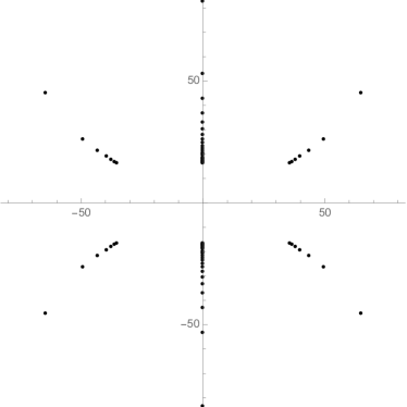
Figure 4: Poles of the Borel–Padé transform of the “reduced” series $\Pi_{B}^{\rm red}$ at $u=4$.

The above analysis suggests that the non-Borel summability of the sequence $\Pi_{B}^{(n)}$ along the positive real axis in the weak coupling region is due to the asymptotic series appearing in $\gamma(a,\hbar)$. In view of (4.159), this leads to the right discontinuity across the positive real axis:

$$-4\hbar\log(1-{\rm e}^{-4\pi a/\hbar}).$$ (4.161)

This suggests that the “reduced” formal power series

$$\Pi^{\text{red}}_{B}(E,\hbar):=\Pi_{B}(E,\hbar)-4{\rm i}\Pi_{A}(E,\hbar)\sum_{n\geq 1}{(-1)^{n}B_{2n}\over 2n(2n-1)}\left({\hbar\over 2\Pi_{A}(E,\hbar)}\right)^{2n},$$ (4.162)

where we subtract the non-Borel summable series in the function $\gamma(a,\hbar)$, is actually Borel summable along the positive real axis. We verified numerically that this indeed is true, as can be seen from the Borel plane plot at $u=4$ given in Figure 4. In fact the Borel sum of $\Pi^{\text{red}}_{B}(E,\hbar)$ agrees with the gauge theory calculation in which the contribution of $\gamma(a,\hbar)$ has been removed; in other words,

$$s\left(\Pi^{\text{red}}_{B}\right)(E,\hbar)=2{\rm i}a_{D}^{\text{red}}(u,\hbar):=4{\rm i}a\left(\log\left(\frac{a}{\Lambda}\right)-1\right)+2{\rm i}\frac{\partial F^{\text{inst}}_{\text{NS}}(a,\hbar)}{\partial a}\ .$$ (4.163)

We illustrate this in Table 9, where both the Borel sum of $\Pi^{\text{red}}_{B}(E,\hbar)$ and $2{\rm i}a_{D}^{\text{red}}(u,\hbar)$ are evaluated at $u=4$ and $\hbar=1$. We find that all stabilised digits are in agreement (26 of them).

We can now see a clear difference between the TBA equations of ns and the TBA equations of gmn . The TBA equations of ns compute the Borel-summable part of the $B$ period, where we have removed the perturbative contribution due to the $\gamma$ function, i.e. they compute (4.163), which is the Borel resummation of $\Pi_{B}^{\rm red}$ in (4.162). On the contrary, the conformal limit of the GMN TBA equations computes the Borel resummation of the full quantum $B$ period $\Pi_{B}(E,\hbar)$, including the perturbative $\gamma$ function. Since the latter is not Borel summable, the corresponding TBA has discontinuities, as discussed in section 3.2.

	terms
$\Pi^{\text{red}}_{B}$	159	16.474810551500808917635392219
	161	16.474810551500808917635392368
$2{\rm i}a_{D}^{\text{red}}$	14	16.47481055150080891763539232909
	15	16.47481055150080891763539232920

Table 9: Comparison between the Borel sum of the “reduced” quantum $B$ period $\Pi^{\text{red}}_{B}$ at $u=4$ and $\hbar=1$ (with increasing number of terms), and the exact, “reduced” period $2{\rm i}a_{D}^{\text{red}}$ defined in (4.163) (with increasing number of instanton corrections). Underlined are stabilised digits.

terms	first line of r.h.s. of (4.164)
191	$806502.11499751621351505261143$
193	$\underline{806502.11499751621351505261}260$
l.h.s. of (4.164)	$806502.11499751621351505261016$

Table 10: Numerical verification of the characteristic exponent formula (4.164) at $u=0$ and $\hbar=1/4$, with increasing number of terms for the lateral Borel resummations on the r.h.s.. All the stabilised digits (underlined) are in agreement.

In the strong coupling region we have the following relation between the “exact” quantum $A$ period and lateral Borel resummations of quantum periods kpt

$$2\cosh(\Pi_{A}^{\text{ex}}/(2\hbar)) ={\rm e}^{\frac{1}{2\hbar}s_{+}(\Pi_{A})}+{\rm e}^{\frac{1}{2\hbar}s_{+}(\Pi_{A}+2\Pi_{B})}+{\rm e}^{-\frac{1}{2\hbar}s_{+}(\Pi_{A}+2\Pi_{B})}$$ (4.164)

$$={\rm e}^{\frac{1}{2\hbar}s_{-}(\Pi_{A})}+{\rm e}^{-\frac{1}{2\hbar}s_{-}(\Pi_{A})}+{\rm e}^{\frac{1}{2\hbar}s_{-}(\Pi_{A}+2\Pi_{B})}\ .$$

Numerical evidence for this relation is presented in Table 10 for the first line of the formula, evaluated at $u=0$ and $\hbar=1/4$. The second line of (4.164) can be derived from the Stokes automorphism of quantum periods discussed in section 3.2. In the strong coupling region, $\Pi_{D}=\Pi_{B}+\Pi_{A}$ is Borel summable along the positive real axis, while both the Borel resummations of $\Pi_{B}$ and $\Pi_{A}$ have discontinuities across the positive real axis. The discontinuities for the $B$, and $A$ periods are:

$$s_{+}(\Pi_{B})-s_{-}(\Pi_{B})=2\hbar\log(1+{\rm e}^{-\frac{1}{\hbar}s(\Pi_{D})})\ ,$$ (4.165)

$$s_{+}(\Pi_{A})-s_{-}(\Pi_{A})=-2\hbar\log(1+{\rm e}^{-\frac{1}{\hbar}s(\Pi_{D})})\ .$$

Starting from the first line on the right hand side of (4.164), and applying the discontinuity formulae, we immediately get the second line

first line

$$={\rm e}^{\frac{1}{2\hbar}s_{+}(\Pi_{A})}+{\rm e}^{\frac{1}{2\hbar}s_{+}(\Pi_{A}+2\Pi_{B})}+{\rm e}^{-\frac{1}{2\hbar}s_{+}(\Pi_{A}+2\Pi_{B})}$$

$$={\rm e}^{\frac{1}{2\hbar}s_{-}(\Pi_{A})}\left(1+{\rm e}^{-\frac{1}{\hbar}s(\Pi_{D})}\right)^{-1}+{\rm e}^{\frac{1}{2\hbar}s_{-}(\Pi_{A}+2\Pi_{B})}\left(1+{\rm e}^{-\frac{1}{\hbar}s(\Pi_{D})}\right)+{\rm e}^{-\frac{1}{2\hbar}s_{-}(\Pi_{A}+2\Pi_{B})}\left(1+{\rm e}^{-\frac{1}{\hbar}s(\Pi_{D})}\right)^{-1}$$

$$=\left({\rm e}^{\frac{1}{2\hbar}s_{-}(\Pi_{A})}+{\rm e}^{-\frac{1}{2\hbar}s_{-}(\Pi_{A}+2\Pi_{B})}\right)\left(1+{\rm e}^{-\frac{1}{\hbar}s(\Pi_{D})}\right)^{-1}+{\rm e}^{\frac{1}{2\hbar}s_{-}(\Pi_{A}+2\Pi_{B})}+{\rm e}^{-\frac{1}{2\hbar}s_{-}(\Pi_{A})}$$

$$={\rm e}^{\frac{1}{2\hbar}s_{-}(\Pi_{A})}+{\rm e}^{-\frac{1}{2\hbar}s_{-}(\Pi_{A})}+{\rm e}^{\frac{1}{2\hbar}s_{-}(\Pi_{A}+2\Pi_{B})}=\text{second line}\ .$$ (4.166)

On the other hand, to derive a similar result for the “exact” quantum $B$ period we can use results on the Fredholm determinant of the modified Mathieu equation, which we present in section 5. Eq.(5.212) then together (4.164) imply that

$$2\sinh(\Pi^{\text{ex}}_{B}/(2\hbar)) ={\rm e}^{\frac{1}{2\hbar}s_{+}(\Pi_{B})}-{\rm e}^{-\frac{1}{2\hbar}s_{+}(\Pi_{B})}-{\rm e}^{-\frac{1}{2\hbar}s_{+}(2\Pi_{A}+3\Pi_{B})},$$ (4.167)

$$={\rm e}^{\frac{1}{2\hbar}s_{-}(\Pi_{B})}-{\rm e}^{-\frac{1}{2\hbar}s_{-}(\Pi_{B})}+{\rm e}^{-\frac{1}{2\hbar}s_{-}(2\Pi_{A}+\Pi_{B})}\ ,$$

and we have tested these identities numerically to very high precision.

Summarizing, in the weak coupling region the all-orders WKB quantum $A$ period and the $B$ period (once the gamma function is subtracted) are Borel summable. Their Borel sums agree with the gauge theory expressions of section 4.1. In the strong coupling region, the $A$ and $B$ periods are not Borel summable, although their lateral Borel resummations can be related to the exact quantum $A$ period via (4.164). We finally note that the combination $\Pi_{D}=\Pi_{A}+\Pi_{B}$ is Borel summable in the strong coupling region (only). However, its Borel sum does not agree with the gauge theory expression of section (4.1), namely

$$s(\Pi_{D})\neq\Pi_{A}^{\rm ex}+\Pi_{B}^{\rm ex}=2\pi a+2{\rm i}a_{D},$$ (4.168)

and one should include additional non-perturbative corrections. We will find the correct formula at the end of section 5.3.

5 The Fredholm determinant from topological string theory

Let $\mathsf{O}$ be an operator on $L^{2}(\mathbb{R})$ such that $\mathsf{O}^{-1}$ is of trace class. Then, $\mathsf{O}$ has a discrete spectrum $\{E_{n}\}_{n\geq 0}$, and its Fredholm determinant

$$\Xi(E)={\rm det}\left(1-E\mathsf{O}^{-1}\right)=\prod_{n\geq 0}\left({1-{E\over E_{n}}}\right)$$ (5.169)

is an entire function of $E$ whose zeros give the spectrum of $\mathsf{O}$: $\Xi(E_{n})=0$ (see e.g. simon-paper for these and other properties of Fredholm determinants).

The Fredholm determinant contains very rich information about the spectral properties of $\mathsf{O}$. For example, the spectral traces, defined as

$$Z_{\ell}=\sum_{n\geq 0}{1\over E_{n}^{\ell}},$$ (5.170)

can be computed by expanding the spectral determinant around $E=0$. Indeed, we have

$$\Xi(E)=\sum_{N\geq 0}(-E)^{N}Z(N,\hbar)$$ (5.171)

where

$$Z(N,\hbar)=\sum_{\{m_{\ell}\}}{}^{{}^{\prime}}\prod_{\ell}{(-1)^{(\ell-1)m_{\ell}}Z_{\ell}^{m_{\ell}}\over m_{\ell}!\ell^{m_{\ell}}},$$ (5.172)

and the ${}^{{}^{\prime}}$ means that the sum is over the integers $m_{\ell}$ satisfying the constraint

$$\sum_{\ell}\ell m_{\ell}=N.$$ (5.173)

From the quantities $Z(N,\hbar)$ (which were called fermionic spectral traces in ghm ) one can extract the conventional spectral traces (5.170).

Although Fredholm determinants are central objects in spectral theory, it is difficult to obtain explicit expressions for them. It is easy to show (see for instance lst ) that the inverse of the modified Mathieu operator (2.14) is of trace class. Therefore, the Fredholm determinant is well-defined, and it is an interesting question to find an explicit, closed form expression for this quantity.

In recent years it was discovered km ; hw ; cgm8 ; ghm ; cgm that, by using topological string tools, it is possible to obtain explicitly expression for Fredholm determinants of operators arising in the context to quantum mirror curves. We will refer to this relationship as the TS/ST correspondence. As explained in section 5.1, the modified Mathieu operator (2.14) can be related, upon a suitable limiting procedure, to the quantum mirror curve of local $\mathbb{F}_{0}$. Therefore we can study (5.169) within the context of topological string theory and in particular, by using ghm ; gm3 , we can deduce an explicit, closed form expression for the Fredholm determinant of the modified Mathieu operator. We will first state the main result and then explain how to derive it within topological string theory. We also present several independent tests of our result, including an interesting connection to the TBA system of post-zamo .

5.1 A closed formula and its derivation

By using the approach of ghm ; gm3 we find the following expression for the spectral determinant of (2.14)

$$\Xi(E)=A(\hbar)\left(\sinh\left(\frac{\Pi_{A}^{\rm ex}(E,\hbar)}{2\hbar}\right)\right)^{-1}\cosh\left({1\over 2\hbar}\Pi_{B}^{\rm ex}(E,\hbar)\right),$$ (5.174)

where $\Pi_{A,B}^{\rm ex}(E,\hbar)$ are given by (4.132) and $A(\hbar)$ is an $u$-independent constant which can be fixed from $\Xi(0)=1$, namely,

$$A(\hbar)=\sinh\left(\frac{\Pi_{A}^{\rm ex}(0,\hbar)}{2\hbar}\right)\left(\cosh\left({1\over 2\hbar}\Pi_{B}^{\rm ex}(0,\hbar)\right)\right)^{-1}.$$ (5.175)

From this expression we can read off explicit formulae for the spectral traces. We find for instance

$$Z_{1}=-{1\over 2\hbar}\left(\partial_{E}\Pi_{B}^{\rm ex}(0,\hbar)\tanh\left({\Pi_{B}^{\rm ex}(0,\hbar)}\over 2\hbar\right)-\coth\left(\frac{\Pi_{A}^{\rm ex}(0,\hbar)}{2\hbar}\right)\partial_{E}\Pi_{A}^{\rm ex}(0,\hbar)\right),$$ (5.176)

as well as

$$4\hbar^{2}Z_{2}= 2\hbar\partial_{E}^{2}\Pi_{A}^{\rm ex}(0,\hbar)\coth\left(\frac{\Pi_{A}^{\rm ex}(0,\hbar)}{2\hbar}\right)-(\partial_{E}\Pi_{A}^{\rm ex}(0,\hbar))^{2}\text{csch}^{2}\left(\frac{\Pi_{A}^{\rm ex}(0,\hbar)}{2\hbar}\right)$$ (5.177)

$$-\text{sech}^{2}\left(\frac{\Pi_{B}^{\rm ex}(0,\hbar)}{2\hbar}\right)\left(\hbar\partial_{E}^{2}\Pi_{B}^{\rm ex}(0,\hbar)\sinh\left(\frac{\Pi_{B}^{\rm ex}(0,\hbar)}{\hbar}\right)+(\partial_{E}\Pi_{B}^{\rm ex}(0,\hbar))^{2}\right).$$

Note that in order to calculate $\Pi_{A}^{\rm ex}(0,\hbar)$ we have to use (4.151) or (4.152), so the above formula tests as well the analytic continuation of instanton calculus beyond the semiclassical region.

The explicit formula (5.174) can be extended to the family of operators considered in gm3 , see Appendix A for more details.

Let us now explain how to derive (5.174) from the TS/ST correspondence of ghm ; cgm . The relevant CY geometry is the canonical bundle over $\mathbb{F}_{0}$, also known as resolved $Y^{2,0}$ singularity. The corresponding quantum mirror curve is

$$\mathsf{O}-\kappa=(R\Lambda)^{2}({\rm e}^{\mathsf{x}}+{\rm e}^{-\mathsf{x}})-\kappa+{\rm e}^{\mathsf{p}}+{\rm e}^{-\mathsf{p}},\quad[\mathsf{x},\mathsf{p}]={\rm i}\hbar.$$ (5.178)

According to the TS/ST correspondence we have

$$\det(1-\kappa\mathsf{O}^{-1})=\sum_{{m}\in\mathbb{Z}}\exp\left[\mathsf{J}({\mu+{\rm i}\pi+2\pi{\rm i}m},R\Lambda,\hbar)\right],\quad\kappa={\rm e}^{\mu},$$ (5.179)

where $\mathsf{J}({\mu},\xi,\hbar)$ is the grand potential of the resolved $Y^{2,0}$ singularity as defined in gm3 , section 5.1. The expression (5.174) is obtained by implementing the geometric engineering limit selfdual ; kkv in (5.179). More precisely, we consider the limit

$$p\to Rp,\quad\hbar\to R\hbar,\quad\kappa=2+ER^{2}+\mathcal{O}(R^{3}),\quad R\to 0.$$ (5.180)

This has to be done carefully since both sides of (5.179) diverge, therefore they need to be properly regularized. For that it is convenient to study the trace of the resolvent

$$G_{\mathsf{O}}(\kappa)={{\rm d}\over{\rm d}\kappa}\log\det(1-\kappa\mathsf{O}^{-1})={\rm Tr}\left({1\over\kappa-\mathsf{O}}\right),$$ (5.181)

rather than the spectral determinant. It is easy to see that in the limit (5.180) one has

$$G_{\mathsf{O}}(\kappa)\to{1\over R^{2}}G(E),\qquad G(E)={\rm Tr}\left({1\over E-\mathsf{H}}\right),$$ (5.182)

where $\mathsf{H}$ is the modified Mathieu operator in (2.14). Likewise the limit (5.180) can be implemented on the r.h.s of (5.179) in a quite straightforward way by following gm3 , section 5.2 and by using the identity (3.9) in bgt . The overall divergent piece $R^{-2}$ cancels and we find

$$G(E)=-{\partial_{E}a\over\hbar}\left(\partial_{a}^{2}F_{\rm NS}\tanh\left({\partial_{a}F_{\rm NS}\over\hbar}\right)+\pi\coth\left({a\pi\over\hbar}\right)\right).$$ (5.183)

By integrating w.r.t. $E$ we obtain (5.174), where $A(\hbar)$ is an integration constant.

5.2 Tests of our formula

We will now test the expression (5.174) in several ways.

A first simple test is that the zeros of $\Xi(E)$ give the correct spectrum of the modified Mathieu operator. This should be expected from the general results of gm3 , but it is instructive to check it explicitly. The zeros correspond to the vanishing of the $\cosh$ in (5.174), and by using (4.132) we find,

$$\partial_{a}F_{\rm NS}(a,\hbar)=\hbar\pi\left(n+{1\over 2}\right),$$ (5.184)

which is the exact quantization condition obtained from the conjecture in ns , subsequently proved in kt2 .

Another check can be obtained by comparing our expression to the asymptotics of Fredholm determinants obtained in voros ; voros-zq ; voros-quartic by using the all-orders WKB method. This asymptotic expansion is valid when $E<0$, where the Fredholm determinant is not oscillatory. In order to write down the asymptotics, we need some ingredients. Let

$$G(E)=\sum_{n=0}^{\infty}{1\over E-E_{n}}$$ (5.185)

be the trace of the resolvent, and

$$T(E)={1\over 2}\int_{\mathbb{R}}{{\rm d}x\over{\sqrt{2\Lambda^{2}\cosh(x)-E}}}$$ (5.186)

the transit time. We also need the formal power series in $\hbar$

$$b(E)=\exp\left\{{\rm i}\sum_{n\geq 1}\hbar^{2n-1}\int_{\mathbb{R}}p_{2n}(x,E){\rm d}x\right\},$$ (5.187)

where the functions $p_{2n}(x,E)$ are the ones appearing in the solution to the all-orders WKB method in (2.4). Let us now define $\kappa=-E$, which will be taken to be positive. It is convenient to introduce the functions

$$\widetilde{G}(\kappa)=G(-\kappa),\qquad\widetilde{\Xi}(\kappa)=\Xi(-\kappa),\qquad\widetilde{b}(\kappa)=b(-\kappa),\qquad\widetilde{T}(\kappa)=T(-\kappa).$$ (5.188)

Then, one has the following small $\hbar$ asymptotics,

$$\widetilde{\Xi}(\kappa)\sim\widetilde{b}(\kappa)\exp\left\{{1\over\hbar}\int_{0}^{\kappa}\widetilde{T}(\kappa^{\prime}){\rm d}\kappa^{\prime}-\int_{0}^{\infty}\left(\widetilde{G}(\kappa^{\prime})+{1\over\hbar}\widetilde{T}(\kappa^{\prime})\right){\rm d}\kappa^{\prime}\right\}.$$ (5.189)

The second term in the exponent is independent of $\kappa$ but depends on $\hbar$. We note that all the integrals involved in this expression are well defined precisely because $E$ is negative. The very first terms in the asymptotics can be easily worked out, and one finds

$$\log\Xi(-\kappa)\sim-{{\rm i}\over 2\hbar}\Pi_{B}^{(0)}(\kappa)+{{\rm i}\hbar\over 2}\Pi_{B}^{(1)}(\kappa)+\cdots,\qquad\kappa>0,$$ (5.190)

up to $\kappa$-independent terms. Note that the sign in the subleading correction is the opposite one to what one finds in the WKB expansion of the quantum $B$ period.

Let us now compare this result to the exact expression for the spectral determinant (5.174), which can be written as

$$\Xi(E)=A(\hbar)\left(\sinh\left(\frac{\pi a}{\hbar}\right)\right)^{-1}\cos\left({1\over\hbar}{\partial F_{\rm NS}\over\partial a}\right).\$$ (5.191)

From the explicit expression (4.142) it is easy to see that, when $E$ is negative, $a$ is purely imaginary. More precisely, one has

$$a(-\kappa,\hbar)={\rm i}\alpha,\qquad\alpha=a(\kappa,{\rm i}\hbar),$$ (5.192)

and we take $\alpha>0$ for definiteness. In addition,

$$\partial_{a}F^{\rm inst}_{\rm NS}(a,\hbar)={\rm i}\partial_{\alpha}F^{\rm inst}_{\rm NS}(\alpha,{\rm i}\hbar).$$ (5.193)

By using the explicit expression (4.130) and standard identities for the $\Gamma$ function, we find

$${\Xi(-\kappa)\over A(\hbar)} ={1\over 2\pi}\Gamma\left(1+{\alpha\over\hbar}\right)\Gamma\left({\alpha\over\hbar}\right)\exp\left[{\alpha\over\hbar}\log\left({\hbar^{2}\over\Lambda^{2}}\right)+{1\over\hbar}\partial_{\alpha}F^{\rm inst}_{\rm NS}(\alpha,{\rm i}\hbar)\right]$$ (5.194)

$$+{1\over 2\pi}\Gamma\left(1-{\alpha\over\hbar}\right)\Gamma\left(-{\alpha\over\hbar}\right)\exp\left[-{\alpha\over\hbar}\log\left({\hbar^{2}\over\Lambda^{2}}\right)-{1\over\hbar}\partial_{\alpha}F^{\rm inst}_{\rm NS}(\alpha,{\rm i}\hbar)\right].$$

The term in the second line gives an exponentially small correction to the leading asymptotics. The small $\hbar$ asymptotics of the quantity in the first line is given by

$$\log\left[{1\over 2\pi}\Gamma\left(1+{\alpha\over\hbar}\right)\Gamma\left({\alpha\over\hbar}\right)\right]+{\alpha\over\hbar}\log\left({\hbar^{2}\over\Lambda^{2}}\right)+{1\over\hbar}\partial_{\alpha}F^{\rm inst}_{\rm NS}(\alpha,{\rm i}\hbar)$$ (5.195)

$$\sim-{{\rm i}\over 2\hbar}\sum_{n\geq 0}(-1)^{n}\Pi_{B}^{(n)}(\kappa)\hbar^{2n}.$$

We have used that, due to (5.192) and (5.193), the quantum period is evaluated at $-E$, where $E=-\kappa<0$, and we have to change $\hbar\rightarrow{\rm i}\hbar$. The result is in agreement with the WKB asymptotics obtained in (5.190).

A more precise test of (5.174) can be made by comparing the analytical formulae for the spectral traces with numerical results. These are obtained by calculating the spectrum of $\mathsf{H}$ with standard techniques. An example of such a comparison is shown in Table 11.

$N_{b}$	$Z_{2}$
2	0.00479478611468342466
4	0.00479478607391381196
6	0.00479478607391375025
Num	0.00479478607391375025

Table 11: The second spectral trace $Z_{2}$ as computed from (5.177) for $\hbar=3\pi$ and $\Lambda=1$. The number $N_{b}$ means that we truncate the series (4.127) at order $\Lambda^{4N_{b}}$. The last line gives the numerical result obtained from the spectrum of $\mathsf{H}$.

We finally note that $\Xi(E)$ is an entire function of $E$. In particular, the would-be singularities due to the denominator of (5.191) or to the Gamma functions in (4.130) must cancel in the end. This leads in turn to constraints on the form of the singularities of $F_{\rm NS}^{\rm inst}$, which might be testable against the results in gorsky-bands (see also beccaria ).

5.3 Comparison to Zamolodchikov’s TBA equation

An additional test of our formula (5.174) comes from a comparison with post-zamo . Inspired by the ODE/IM correspondence dt ; ddt , Zamolodchikov found in post-zamo a TBA equation which computes precisely the spectral determinant (5.174). Let us state the main result of post-zamo , referring to Appendix B for more details. Let $\epsilon(\theta,P)$ be a solution of the TBA equation (3.103) but with the boundary condition at $\theta\rightarrow-\infty$ given by

$$\epsilon(\theta,P)\sim 8P\theta-2C(P),\qquad\theta\to-\infty,\quad P>0,$$ (5.196)

where $C(P)$ is written down in (B.247). Let us now introduce the function

$$X(\mu,P)=\exp\left[-\epsilon(\theta,P)/2\right],$$ (5.197)

where $\mu$ is related to $\theta$ by

$$\mu={\rm e}^{2\theta}\left(\frac{\Gamma\left(\frac{1}{4}\right)^{2}}{16\sqrt{\pi}}\right)^{2}.$$ (5.198)

Then, according to post-zamo , the spectral determinant of the modified Mathieu operator (2.14) is given by

$$\Xi(E)={X(\mu,P)\over X(\mu,0)},$$ (5.199)

where the parameters $\Lambda$, $E$ and $\hbar$ of the operator are related to the parameters appearing in $X(\mu,P)$ by

$$\mu=\Lambda^{2}\hbar^{-2},\qquad P^{2}=-E\hbar^{-2}.$$ (5.200)

If we compare the result of post-zamo with ours we should have (by using the dictionary (5.200))

$${X(\mu,P)\over X(\mu,0)}=A(\hbar)\left(\sinh\left(\frac{\Pi_{A}^{\rm ex}(E,\hbar)}{2\hbar}\right)\right)^{-1}\cosh\left({1\over 2\hbar}\Pi_{B}^{\rm ex}(E,\hbar)\right).$$ (5.201)

In order to find the relation between the two normalization constants $X(\mu,0)$ and $A(\hbar)$, it is useful to first derive the asymptotic behavior (5.196) from our expression (5.174). We need to expand around small $\Lambda\hbar^{-1}$ and take $u<0$, which means that $a$ is imaginary, as discussed in (5.192). In this regime, and by using (4.132), we have

$$\left(\sinh\left(\frac{\pi a}{\hbar}\right)\right)^{-1}\cosh\left({{\rm i}\over\hbar}\partial_{a}F_{\rm NS}(a,\hbar)\right)$$ (5.202)

$$\approx 2^{-1}\pi^{-1}\left(\left({\Lambda\over\hbar}\right)^{-2s}\Gamma(1+s)\Gamma(s)+\left({\Lambda\over\hbar}\right)^{2s}\Gamma(1-s)\Gamma(-s)\right),$$

where

$$s=-{\rm i}{a\over\hbar}=\frac{\alpha}{\hbar}>0.$$ (5.203)

By using (4.128) we have

$$E\approx a^{2}/4$$ (5.204)

and therefore

$$P=s/2>0.$$ (5.205)

Hence we can neglect the second term in the r.h.s. of (5.202). It follows from (5.200) that (5.202) agrees precisely with (5.196). In particular this means that the two normalization constants are identified and we have

$$X(\mu,P)=\left(\sinh\left(\frac{\Pi_{A}^{\rm ex}(E,\hbar)}{2\hbar}\right)\right)^{-1}\cosh\left({1\over 2\hbar}\Pi_{B}^{\rm ex}(E,\hbar)\right).$$ (5.206)

We test this equality by solving numerically the TBA equation (3.103) with the boundary condition (5.196). Some results are given in Table 12. We find perfect agreement.

$N_{b}$	$\log\left(\left(\sinh\left(\frac{\pi a}{\hbar}\right)\right)^{-1}\cosh\left({{\rm i}\over\hbar}\partial_{a}F_{\rm NS}(a,\hbar)\right)\right)$
2	11.360025317439438
4	11.360025299112863
6	11.360025299117259
TBA	11.360025299117

Table 12: The un-normalized spectral determinant as computed by using instanton counting and by solving numerically the TBA (3.103) with (5.196). We use $P^{2}=-E=5$, $\mu=\Lambda^{2}=\left(\Gamma\left(1/4\right)^{2}/(16\sqrt{\pi})\right)^{2}$, and $\hbar=1$. The number $N_{b}$ means that we truncate the series (4.127) at order $\Lambda^{4N_{b}}$.

An important spinoff of this comparison is that our result (5.174) provides an analytic, closed form solution to the TBA equation of post-zamo . This also has the following consequence. When we derived the Fredholm determinant from the topological string perspective, and due to our regularization procedure, we generated an integration constant $A(\hbar)$ whose explicit expression is given in (5.175). Given the identity (5.206) between our Fredholm determinant and the solution to the Zamolodchikov’s TBA, we expect $A(\hbar)$ to be computed by the integral equation (3.103) at $P=u=0$. More precisely we expect

$$2\log A(\hbar)=\epsilon(\theta,P=0),$$ (5.207)

where we used the dictionary (5.200). For $P=0$ the asymptotic condition (5.196) does not make sense, strictly speaking. Nevertheless, we can derive the appropriate asymptotic condition for the TBA at $P=0$ by using our analytic expression (5.206). We find that, as $\theta\rightarrow-\infty$,

$$\epsilon(\theta,P=0)\sim-2\log\left(-\frac{2(\theta+\gamma_{\rm Euler})-\log\pi+4\log\Gamma(5/4)}{\pi}\right).$$ (5.208)

This is precisely the boundary condition used in section 3.3, equation (3.108). One can now check (5.207) numerically. For instance, by solving the TBA of section 3.3 we find

$$\epsilon(\theta,P=0)\Big{|}_{\theta=-1}=0.51888\cdots$$ (5.209)

Likewise, by using instanton counting, and in particular (4.132) and (5.175), we have ($\Lambda=1$)

$$2\log\left(A\left(\frac{16{\rm e}\sqrt{\pi}}{\Gamma\left(\frac{1}{4}\right)^{2}}\right)\right)=0.51887965286656\cdots$$ (5.210)

We have 5 matching digits which is consistent with the precision achieved with the TBA equation.

This discussion provides an additional result along the lines of what we obtained in section 4.2. As we discussed in section 3.3, the function $\epsilon(\theta)$ with the boundary condition (3.108) computes the dyonic period $\Pi_{D}(0,\hbar)$. As pointed out in Sec 4.2, such period is Borel summable, and we can indeed test that its Borel resummation agrees with (5.175), namely

$$\exp\left({1\over 2\hbar}s\left(\Pi_{D}\right)(0,\hbar)\right)={\sinh\left(\frac{\pi a}{\hbar}\right)\over\cosh\left({{\rm i}\over\hbar}\partial_{a}F_{\rm NS}(a,\hbar)\right)}\bigg{|}_{a=a(0,\hbar)}=\frac{\sinh\left(\frac{1}{2\hbar}\Pi_{A}^{\rm ex}(0,\hbar)\right)}{\cosh\left({1\over 2\hbar}\Pi_{B}^{\rm ex}(0,\hbar)\right)}.$$ (5.211)

We have verified this identity numerically. In addition we have tested that (5.211) also holds for other values of $u$ in the strong coupling region, and we conjecture that, for $u\in[-1,1]$, one has

$$\exp\left({1\over 2\hbar}s\left(\Pi_{D}\right)(u,\hbar)\right)=\frac{\sinh\left(\frac{1}{2\hbar}\Pi_{A}^{\rm ex}(u,\hbar)\right)}{\cosh\left({1\over 2\hbar}\Pi_{B}^{\rm ex}(u,\hbar)\right)}.$$ (5.212)

6 On the modified Mathieu operator and Painlevé $\rm III_{3}$

It was observed by many authors Lukyanov:2011wd ; PCL ; nok that the movable poles of Painlevé $\rm III_{3}$ are somehow related to Mathieu functions. In particular in sciarappa2 , based on bgt , it was observed that the zeros of the Painlevé $\rm III_{3}$ $\tau$ function compute the spectrum of modified Mathieu (with a suitable dictionary). From the view point of the TS/ST correspondence ghm this connection comes naturally since both systems arise as limiting cases of this duality. In particular, the modified Mathieu operator arises in the standard geometric engineering limit hm ; gm17 ; gm3 , while Painlevé $\rm III_{3}$ arises in the dual geometric engineering limit considered in bgt .

In this section we prove the connection between the zeros of the Painlevé $\rm III_{3}$ $\tau$ function and the spectrum of the modified Mathieu operator by using ggu . From the CFT perspective this is a connection between Liouville conformal blocks at $c=1$ and $c=\infty$. We proceed as follows. First we write the Painlevé $\rm III_{3}$ $\tau$ function as gil ; ilt ; Gavrylenko:2017lqz

$$\tau(\Lambda,a,\eta,\hbar)=\sum_{n\in\mathbb{Z}}{\rm e}^{4\pi{\rm i}n\eta}\exp\left(F^{\rm SD}(a+2{\rm i}\hbar n,\hbar,\Lambda)\right)$$ (6.213)

where

$$\exp\left(F^{\rm SD}(a,\hbar,\Lambda)\right)= \left(\frac{\Lambda}{\hbar}\right)^{-\frac{a^{2}}{\hbar^{2}}}{1\over G(1-{\rm i}\frac{a}{\hbar})G(1+{\rm i}\frac{a}{\hbar})}$$ (6.214)

$$\times\left(1-\frac{2\Lambda^{4}}{a^{2}\hbar^{2}}+\frac{\Lambda^{8}\left(2a^{2}-\hbar^{2}\right)}{a^{2}\hbar^{2}\left(a^{2}+\hbar^{2}\right)^{2}}+\mathcal{O}(\Lambda^{12})\right)$$

is the so-called four dimensional Nekrasov partition function in the selfdual $\Omega$ background n (namely, the equivariant parameters are $\epsilon_{1}=-\epsilon_{2}=\hbar$). The parameters $(a,\eta)$ in (6.213) play the role of initial conditions while $\Lambda$ is the time. We are interested in the case in which

$$\eta=0.$$ (6.215)

We now recall the result of ggu , where it was demonstrated that, in the NS limit, the Nakajima–Yoshioka blowup equations for $SU(2)$ pure SYM ny1 ; naga ; nagalect can be written as

$$\sum_{n\in\mathbb{Z}}\exp\left({\rm i}n\pi+{F}^{\rm SD}\left(a+2{\rm i}\hbar n+{\rm i}\hbar,\hbar,\Lambda\right)-2{\rm i}n\hbar^{-1}\frac{\partial}{\partial a}{F}_{\text{NS}}\left(a,\hbar\right)\right)=0.$$ (6.216)

Finally, we use the quantization condition for the modified Mathieu operator in the NS form (5.184). It then follows from (6.216) that, if a value of $a$ satisfies this exact quantization condition, one finds a vanishing condition for the tau function of Painlevé $\rm III_{3}$, namely

$$\tau\left(\Lambda,a+{{\rm i}\hbar},0,\hbar\right)=\sum_{n\in\mathbb{Z}}\exp\left({F}^{\rm SD}\left(a+2{\rm i}\hbar n+{\rm i}\hbar,\hbar,\Lambda\right)\right)=0.$$ (6.217)

Notice that we think of (5.184) and (6.217) as quantization conditions for the variable $a$. In order to obtain the spectrum of modified Mathieu one has to use the quantum Matone relation (4.128).

7 Conclusions

In this paper we have used non-perturbative techniques inspired by supersymmetric gauge theory and topological string theory to study the quantization of the Seiberg–Witten curve of ${\cal N}=2$, $SU(2)$ super Yang–Mills theory, which gives the modified Mathieu operator. On the one hand, building upon gmn ; gmn2 ; oper ; ims , we have obtained integral equations for the Borel resummation of the quantum periods obtained with the all-orders WKB method. These equations predict as well the resurgent structure of these periods, and in particular their Stokes discontinuities. The results obtained in this way have been tested against calculations in the WKB method to very high order. We have also clarified the relation between these Borel-resummed quantum periods and the “exact” quantum periods given by instanton calculus (in the NS limit). On the other hand, we have used the TS/ST correspondence of ghm ; cgm to obtain a closed formula for the spectral determinant of the modified Mathieu operator, and we have compared this formula to previous results by Zamolodchikov.

Our results raise several issues. An important problem concerns the relation between the TBA equations obtained in the context of SW theory, and the analytic bootstrap program first proposed in voros-quartic and reloaded in ims ; mm-s2019 . In the TBA equations obtained in oper ; ims for quantum mechanics with polynomial potentials, one only needs the boundary condition associated to the classical behavior (i.e. at $\hbar\rightarrow 0$, or equivalently at $\theta\rightarrow\infty$). The boundary behavior when $\theta\rightarrow-\infty$ is fixed by the integral equations. As pointed out already in oper and further discussed in section 3.3 of this paper, the integral equations for the modified Mathieu operator admit many possible boundary conditions at $\theta\rightarrow-\infty$, and one needs additional information to fix them. One can use the quantum Matone relation and the first quantum correction to the periods to obtain additional constraints. However, it seems clear from the study of this example that the analytic bootstrap might require additional asymptotic information to determine uniquely the resummed quantum periods. As suggested in oper , one might obtain the appropriate boundary conditions by first solving the full TBA equations of gmn (before taking the conformal limit) and then implementing the conformal limit directly on the solution.

Another problem that should be discussed more carefully is how to solve efficiently the TBA equations to compute the Borel resummed quantum periods. In particular, we should understand in detail how to to solve the infinite tower of TBA equations appearing in the weak coupling region.

It would be very interesting to extend the techniques developed in this paper to quantum mirror curves. This would provide a relation between BPS states in local CY threefolds (studied for example in dfr ) and the resurgent properties of the corresponding quantum periods. Work along this direction has been already done in eager ; longhi . Another interesting class of quantum curves which could be studied with our methods is the one given by quantum A-polynomials of knots (see e.g. exact-dimofte ). In this case, the resurgent properties should be closely related to the resurgent properties of Andersen–Kashaev invariants ak , which have been considered in gmp ; gh ; andersen . They might correspond to BPS states in the supersymmetric dual obtained with the 3d/3d correspondence of dgg .

Another intriguing point is the following. Based on previous works oper ; ims , we have shown that the conformal limit of the GMN TBA equations encode in a precise way the NS limit of the Omega background for the pure SU(2) theory. On the other hand it is interesting to observe that, as pointed out in bgt , there is another set of TBA equations which computes the selfdual limit of the Omega background. The latter was obtained by Zamolodchikov in zamo , see also Fendley:1999zd . Interestingly also such TBA can be obtained from gmn upon a suitable limiting procedure. It would be interesting to investigate more concretely if and how the full TBA equations of gmn encode the full Omega background. Work along this direction was performed in Cecotti:2014wea .

In addition it should be possible to extend the results of section 6 to Painlevé $\rm III_{2},III_{1},V$ and $\rm VI$. In these cases, the rôle of the modified Mathieu operator is replaced by the quantum SW curve of $SU(2)$ gauge theory with $N_{f}=1,2,3,4$ flavours, respectively. In particular, for $N_{f}=4$ one should recover the connection between Painlevé $\rm VI$ and the Heun operator Litvinov:2013sxa (see also Lencses:2017dgf ). Likewise the spectrum of the Calogero-Moser system should make contact with the $\tau$ function describing the isomonodromic deformations on the torus Bonelli:2019boe . The details will appear somewhere else BGG-p .

The situation for Painlevé $\rm I,II,IV$ is more subtle since these correspond to Argyres–Douglas theories of type $H_{0},H_{1},H_{2}$, respectively blmst . At present we do not know how to write Nakajima-Yoshioka blowup equations for these theories. Nevertheless, it should be possible to connect the NS limit to the selfdual limit of the $\Omega$ background also in these theories, since the $H_{i}$ theories can be derived from $SU(2)$ gauge theories with $N_{f}=1,2,3$ upon a suitable limiting procedure ad ; Argyres:1995xn . By following gg-qm ; ito-shu , such connection would provide a relation between the exact spectrum of the quantum SW curves underlying the $H_{0},H_{1},H_{2}$ theories, and Painlevé $\rm I,II,IV$ tau functions. Note that the quantum SW curve of the $H_{0}$ and $H_{1}$ theories correspond to the cubic and quartic oscillators, respectively. Connections between Painlevé equations and the above quantum mechanical systems have been observed in dm1 ; dm2 ; nok2 ; bender-painleve .

Appendix A The four dimensional $SU(N)$ spectral determinant

In this Appendix we explain how the exact formula (5.174) can be extended to the family of operators studied in gm3 . These operators have the form,

$$\mathsf{H}_{N}=\Lambda^{N}\left({\rm e}^{\mathsf{p}}+{\rm e}^{-\mathsf{p}}\right)+\sum_{k=0}^{N-1}(-1)^{k}\mathsf{x}^{N-k}h_{k},\quad[\mathsf{x},\mathsf{p}]={\rm i}\hbar,$$ (A.218)

where $N\geq 2$ is a positive integer and we set $h_{0}=1$, $h_{1}=0$. They can be regarded as deformations of the standard non-relativistic Schrödinger operators with a polynomial potential. When $N$ is even, they have a discrete spectrum and their inverses are of trace class. When $N$ is odd, one can perform a standard analytic continuation and obtain a discrete spectrum of resonances, as explained in gm3 . In both cases, one can define a Fredholm determinant as

$$\Xi_{N}(h_{2},\cdots,h_{N})=\det\left(1+{h_{N}(-1)^{N}\over\mathsf{H}_{N}}\right).$$ (A.219)

Here, $h_{2},\cdots,h_{N-1}$ are the moduli appearing in the potential, while $(-1)^{N-1}h_{N}$ can be identified with the energy and is the standard auxiliary variable appearing in the definition of Fredholm determinants.

As explained in gm3 , we can engineer the following operator from the quantum mirror curve to the $Y^{N,0}$ geometry. We follow gm3 and define

$$\boldsymbol{\gamma}={1\over 2}\sum_{i=1}^{N}(-1)^{i-1}\boldsymbol{e}_{i},$$ (A.220)

where $\boldsymbol{e}_{i}$ are the weights of the fundamental representation of $SU(N)$. We denote by

$${\cal W}_{N}\cdot\boldsymbol{\gamma}=\left\{w(\boldsymbol{\gamma}):w\in{\cal W}_{N}\right\}$$ (A.221)

the Weyl orbit of $\boldsymbol{\gamma}$, and we introduce

$$\boldsymbol{a}=\sum_{j=1}^{N-1}a_{i}\boldsymbol{\lambda},$$ (A.222)

where $\{\boldsymbol{\lambda}_{i}\}_{i=1,\cdots,N-1}$ are the fundamental weights of $SU(N)$. The quantities $a_{i}$ are related to the parameters $h_{i}$ in (A.218) by using the four dimensional mirror maps or quantum Matone relations (see for instance eqs (3.95)–(3.107) in gm3 and reference therein). For instance, we have

$$h_{2}\left(\boldsymbol{a};\hbar\right) =\lim_{\epsilon_{2}\to 0}\left(-{1\over Z}\sum_{\boldsymbol{Y}}\left((-1)^{N}\Lambda^{2N}\right)^{\ell(\boldsymbol{Y})}{\cal C}_{2}(\boldsymbol{a},\boldsymbol{Y}){\cal Z}_{\boldsymbol{Y}}\right),$$ (A.223)

$$h_{3}\left(\boldsymbol{a};\hbar\right) =\lim_{\epsilon_{2}\to 0}\left({2\over Z}\sum_{\boldsymbol{Y}}\left((-1)^{N}\Lambda^{2N}\right)^{\ell(\boldsymbol{Y})}{\cal C}_{3}(\boldsymbol{a},\boldsymbol{Y}){\cal Z}_{\boldsymbol{Y}}\right),$$

where ${\cal Z}_{\boldsymbol{Y}},Z$ are defined in (4.123) and (4.122), and $\boldsymbol{Y}$ is a vector of Young diagrams as in (4.118). Moreover,

$${\cal C}_{2}(\boldsymbol{a},\boldsymbol{Y}) ={1\over 2}\sum_{I=1}^{N}\alpha_{I}^{2}-{\rm i}\hbar\epsilon_{2}\ell(\boldsymbol{Y}),$$ (A.224)

$${\cal C}_{3}(\boldsymbol{a},\boldsymbol{Y}) ={\rm i}\hbar\epsilon_{2}\left({{\rm i}\hbar+\epsilon_{2}\over 2}\ell(\boldsymbol{Y})+{\rm i}\hbar\sum_{I=1}^{N}c_{2}(Y^{t}_{I})+\epsilon_{2}\sum_{I=1}^{N}c_{2}(Y_{I})-\sum_{I=1}^{N}\alpha_{I}\ell(Y_{I})\right)$$

$$+{1\over 6}\sum_{I=1}^{N}\alpha_{I}^{3},$$

where $\ell(\boldsymbol{Y})$ is defined in (4.120) and we use

$$c_{2}(Y)={1\over 2}\sum_{i\geq 1}y_{i}(y_{i}-1).$$ (A.225)

We also denote

$$a_{i}=\alpha_{i}-\alpha_{i+1},\quad i=1,\cdots,N-1,$$ (A.226)

with

$$\sum_{i=1}^{N}\alpha_{i}=0.$$ (A.227)

With a procedure analogous to the one of section 5.1, we obtain the explicit formula

$$\Xi_{N}(h_{2},\cdots,h_{N})=A_{N}(\hbar,\Lambda,{h_{2}},\cdots h_{N-1})\sum_{{\bf n}\in{\cal W}_{N}\cdot\boldsymbol{\gamma}}{\rm e}^{J_{\boldsymbol{n}}^{\rm 4d}}.$$ (A.228)

The quantity ${\rm e}^{J_{\boldsymbol{n}}^{\rm 4d}}$ is defined as follows. If $N$ is even we have:

$${\rm e}^{J_{\boldsymbol{n}}^{\rm 4d}}=\exp\left({{\rm i}\over\hbar}{\partial F_{\rm NS}\over\partial\boldsymbol{a}}\cdot\boldsymbol{n}\right)\prod_{\alpha\in\Delta_{+}}\left(2\sinh\left({\pi\boldsymbol{a}\cdot\boldsymbol{\alpha}\over\hbar}\right)\right)^{-\left(\boldsymbol{n}\cdot\boldsymbol{\alpha}\right)^{2}},$$ (A.229)

while if $N$ is odd we have

$${\rm e}^{J_{\boldsymbol{n}}^{\rm 4d}}=\exp\left({{\rm i}\over\hbar}{\partial F_{\rm NS}\over\partial\boldsymbol{a}}\cdot\boldsymbol{n}-{\pi\over\hbar}\boldsymbol{a}\cdot\boldsymbol{n}\right)\prod_{\alpha\in\Delta_{+}}\left(2\sinh\left({\pi\boldsymbol{a}\cdot\boldsymbol{\alpha}\over\hbar}\right)\right)^{-\left(\boldsymbol{n}\cdot\boldsymbol{\alpha}\right)^{2}},$$ (A.230)

where $F_{\rm NS}$ is defined in (4.126). The quantity $A_{N}(\hbar,\Lambda,{h_{2}},\cdots h_{N-1})$ is an integration constant, analogous to $A(\hbar)$ in (5.174), which now depends on the moduli $h_{2},\cdots,h_{N-1}$. The above spectral determinant vanishes precisely when the quantization conditions obtained in gm3 are satisfied. When $N=2$ we recover exactly the result (5.174). When $N=3$ we have

$$\Xi_{3}(h_{3},h_{2}) =A_{3}(\hbar,\Lambda,h_{2})\left[1+{1-{\rm e}^{-2\pi a_{1}/\hbar}\over 1-{\rm e}^{-2\pi(a_{1}+a_{2})/\hbar}}{\rm e}^{-2\pi a_{2}/\hbar}{\rm e}^{{\rm i}\phi_{2}}+{1-{\rm e}^{-2\pi a_{2}/\hbar}\over 1-{\rm e}^{-2\pi(a_{1}+a_{2})/\hbar}}{\rm e}^{{\rm i}\phi_{1}}\right]$$ (A.231)

$$\times\text{csch}\left(\frac{\pi a_{1}}{\hbar}\right)\text{csch}\left(\frac{\pi a_{2}}{\hbar}\right){\rm e}^{-\frac{\pi(a_{1}-a_{2})}{3\hbar}-{\rm i}{1\over 3}(\phi_{1}+\phi_{2})},$$

where $\phi_{i}$, $i=1,2$, are defined as gm3

$$\phi_{1}(a_{1},a_{2};\hbar)={1\over\hbar}\left({\partial F_{\rm NS}\over\partial a_{2}}-2{\partial F_{\rm NS}\over\partial a_{1}}\right),\qquad\phi_{2}(a_{1},a_{2};\hbar)={1\over\hbar}\left(2{\partial F_{\rm NS}\over\partial a_{2}}-{\partial F_{\rm NS}\over\partial a_{1}}\right).$$ (A.232)

We have tested (A.231) by expanding the r.h.s of (A.231) around $h_{3}=0$ and comparing with the numerical values of the spectral traces. We find perfect agreement.

Appendix B Zamolodchikov’s TBA equation for the modified Mathieu equation

In zamo-sg Zamolodchikov considered the thermodynamic TBA ansatz for the sinh-Gordon model. This model depends on the parameter $b\in\mathbb{C}$, and we introduce

$$Q=b+{1\over b},$$ (B.233)

as well as

$$p={b^{2}\over 1+b^{2}},\qquad a=1-2p={1-b^{2}\over 1+b^{2}}.$$ (B.234)

The TBA equation for this theory is given by

$$\epsilon(\theta)=mR\cosh(\theta)-\left(\phi\star L\right)(\theta),$$ (B.235)

In this equation, $R$ is the radius of the circle where the theory lives, $m$ is the mass of the particle in the spectrum,

$$L(\theta)=\log\left(1+{\rm e}^{-\epsilon(\theta)}\right),$$ (B.236)

and

$$\phi(\theta)={1\over 2\pi}\left({1\over\cosh(\theta-{\rm i}\pi a/2)}+{1\over\cosh(\theta+{\rm i}\pi a/2)}\right)={1\over 2\pi}{4\sin(\pi p)\cosh(\theta)\over\cosh(2\theta)-\cos(2\pi p)}.$$ (B.237)

The $\star$ in (B.235) denotes, as it is standard, the convolution

$$\left(f\star g\right)(\theta)=\int_{\mathbb{R}}f(\theta-\theta^{\prime})g(\theta^{\prime}){\rm d}\theta^{\prime}.$$ (B.238)

The ground state energy is then given by

$$E(R)=-{m\over 2\pi}\int_{\mathbb{R}}\cosh(\theta)L(\theta){\rm d}\theta,$$ (B.239)

and the effective central charge is

$$c_{\rm eff}=-{6R\over\pi}E(R).$$ (B.240)

The formal conformal limit of the above TBA equation was analyzed in post-zamo in relation to the generalized Mathieu equation

$$-u^{\prime\prime}(x)+\left(\mu_{-}{\rm e}^{-bx}+\mu_{+}{\rm e}^{bx}\right)u(x)=-P^{2}u(x).$$ (B.241)

The parameters $\mu_{\pm}$ have the following obvious symmetry

$$\mu_{+}\to\mu_{+}{\rm e}^{-\varepsilon/b}\ ,\quad\mu_{-}\to\mu_{-}{\rm e}^{+\varepsilon b}\ ,\quad x\to x+\varepsilon\ ,$$ (B.242)

and therefore only the combination

$$\mu=\mu_{+}^{b}\mu_{-}^{1/b}$$ (B.243)

matters. The parameter $b$ is identified with the parameter of the sinh-Gordon model, $\mu$ corresponds to its coupling constant, while the energy

$$E=-P^{2}$$ (B.244)

is identified with the Liouville momentum, and enters into the effective central charge of the theory, see (B.260). In the conformal limit, the TBA equation (B.235) becomes

$$\epsilon(\theta)=\pi{\rm e}^{\theta}-2\left(\phi\star L\right)(\theta).$$ (B.245)

The dependence on $P$ comes through as the boundary condition of the TBA solution when $\theta\rightarrow-\infty$,

$$\epsilon(\theta)\sim 4QP\theta-2C(P)+\cdots$$ (B.246)

where $P>0$ and

$$C(P)=\log\frac{\Gamma(2P)\Gamma(1+2P)}{2\pi}+4P\log\frac{16\sqrt{\pi}}{\Gamma(1/4)^{2}}\ .$$ (B.247)

It is then argued in zamo-sg that the Fredholm determinant of the generalized Mathieu equation is given by post-zamo

$$\Xi(\mu,P)={X(\mu,P)\over X(\mu,0)},$$ (B.248)

where

$$X(\mu,P)=\exp\left[-\epsilon(\theta,P)/2\right]$$ (B.249)

and $\mu$ is related to $\theta$ by (5.198). We have indicated the explicit dependence of $\epsilon$ on $P$ through the boundary condition (B.246).

The ordinary modified Mathieu equation is obtained when

$$b=1,\qquad\mu_{-}=\mu_{+}=\mu.$$ (B.250)

Let us focus on this case. The TBA equation becomes

$$\epsilon(\theta)=\pi{\rm e}^{\theta}-\int_{\mathbb{R}}{L(\theta^{\prime})\over\cosh(\theta-\theta^{\prime})}{{\rm d}\theta^{\prime}\over\pi}.$$ (B.251)

To impose the boundary condition (B.246), we use a trick due to Zamolodchikov. We first note that, as a consequence of (B.246), we have

$$L(\theta)\sim-8P\theta+2C(P),\qquad\theta\rightarrow-\infty,$$ (B.252)

and we introduce the function

$$L_{0}(\theta)=4P\log(1+{\rm e}^{-2\theta}),$$ (B.253)

which has the same leading asymptotics than $L(\theta)$,

$$L_{0}(\theta)\sim-8P\theta+{\cal O}({\rm e}^{-|\theta|}),\qquad\theta\rightarrow-\infty.$$ (B.254)

We have

$$f_{0}=2\phi\star L_{0}=8P\log(1+{\rm e}^{-\theta}),$$ (B.255)

and we can rewrite the TBA equation as

$$\epsilon(\theta)=\pi{\rm e}^{\theta}-f_{0}-2\phi\star(L-L_{0}).$$ (B.256)

This has by construction the right asymptotic behavior (B.246).

One property of (B.251) which is relevant for our analysis is the following. The asymptotic behavior of the solution $\epsilon(\theta)$ as $\theta\rightarrow\infty$ is of the form

$$\epsilon(\theta)=\pi{\rm e}^{\theta}+\epsilon^{(1)}{\rm e}^{-\theta}+\cdots,$$ (B.257)

where

$$\epsilon^{(1)}=-{2\over\pi}\int_{\mathbb{R}}{\rm e}^{\theta}\log\left(1+{\rm e}^{-\epsilon(\theta)}\right){\rm d}\theta.$$ (B.258)

On the other hand, this correction is proportional to the effective central charge of the theory,

$$c_{\rm eff}={6\over\pi}\int_{\mathbb{R}}{\rm e}^{\theta}\log\left(1+{\rm e}^{-\epsilon(\theta)}\right){\rm d}\theta=-3\epsilon^{(1)},$$ (B.259)

which according to post-zamo can be computed in terms of $P$ only

$$c_{\rm eff}=1+24P^{2}.$$ (B.260)

This means that

$$\epsilon^{(1)}=-{1\over 3}\left(1+24P^{2}\right).$$ (B.261)