Inflation in Supergravity from Field Redefinitions

Abstract

Supergravity (SUGRA) theories are specified by a few functions, most notably the real Kähler function denoted by $G(T_{i},\bar{T}_{i})=K+\log|W|^{2}$, where K is a real Kähler potential, and W is a holomorphic superpotential. A field redefinition $T_{i}\rightarrow f_{1}(T_{i})$ changes neither the theory nor the Kähler geometry. Similarly, the Kähler transformation, $K\rightarrow K+f_{2}+\bar{f}_{2},W\rightarrow e^{-f_{2}}W$ where $f_{2}$ is holomorphic and leaves G and hence the theory and the geometry invariant. However, if we perform a field redefinition only in $K(T_{i},\bar{T}_{i})\rightarrow K(f(T_{i}),f(\bar{T}_{i}))$, while keeping the same superpotential $W(T_{i})$, we get a different theory, as G is not invariant under such a transformation while maintaining the same Kähler geometry. This freedom of choosing $f(T_{i})$ allows construction of an infinite number of new theories given a fixed Kähler geometry and a predetermined superpotential W. Our construction generalizes previous ones that were limited by the holomorphic property of $W$. In particular, it allows for novel inflationary SUGRA models and particle phenomenology model building, where the different models correspond to different choices of field redefinitions. We demonstrate this possibility by constructing several prototypes of inflationary models (hilltop, Starobinsky-like, plateau, log-squared and bell-curve) all in flat Kähler geometry and an originally renormalizable superpotential $W$. The models are in accord with current observations and predict $r\in[10^{-6},0.06]$ spanning several decades that can be easily obtained. In the bell-curve model, there also exists a built-in gravitational reheating mechanism with $T_{R}\sim\mathcal{O}(10^{7}GeV)$.

I Introduction

Cosmic inflation Starobinsky:1980te ; Lyth:1998xn ; Sato:1980yn is a hypothetical period of accelerated expansion of the Universe. Inflation solves certain problems of classical cosmology Guth:1980zm and is responsible for generating the primordial inhomogeneities of the Universe. Predictions of inflation are also highly consistent with experimental data Akrami:2018odb . Inflation usually requires flat potentials or flat directions in field space (for single and multi-field inflationary models respectively), which appear naturally in Supersymmetry (SUSY) and Supergravity (SUGRA). On the other hand, the well-known eta-problem is most clearly evident in SUGRA, where canonical Kähler potential of the form $K=T\bar{T}$ immediately generates a very steep potential along the radial direction of the field due to the exponential nature of the scalar potential $V=e^{K}(\cdots)$. In the last decade many SUGRA inflationary models have been developed, with the emphasis on the $\alpha$-attractors Kallosh:2013yoa ; Artymowski:2016pjz ; Dimopoulos:2016yep , for which a non-canonical Kähler potential generates a kinetic term with a pole and, in consequence, a scalar potential with an inflationary plateau.

$\alpha$-attractors are characterized by Kähler potentials with non-zero Kähler curvature. Such a non-canonical Kähler potential generally assumes some knowledge of the UV theory, and restricts the possible UV completions. An alternative to this approach is to investigate Kähler potentials of flat geometry with $\mathcal{R}_{i\bar{j}k\bar{l}}=0$. For instance, Kawasaki:2000yn

$$K_{\pm}=\pm\frac{1}{2}\left(T\pm\bar{T}\right)^{2}+S\bar{S}.$$ (1)

Such a Kähler potential gives the scalars canonical kinetic terms and can always be viewed as a low energy approximation of some UV complete model without restrictions. Obviously, such a Kähler potential has a flat Kähler direction along $T_{R}\equiv\Re{T}$ $(T_{I}\equiv\Im{T})$ for $-$ $(+)$ in (1). One can use this flat direction to generate inflation. The crucial ingredient is the shift symmetry of the Kähler potential, $T\rightarrow T\pm c$ for pure imaginary (real) $c$. Generalization of this form of Kähler potentials has been used throughout the literature. Generalizations beyond the simple shift symmetry of singlets to Higgs doublets and other symmetry groups have been suggested in BenDayan:2010yz ; Nakayama:2010sk .

The existing SUGRA literature connects the possibility and the type of model of inflation with the Kähler geometry. Perhaps the well-known examples are necessary conditions on the sectional curvature of the Kähler manifold Badziak:2008yg ; BenDayan:2008dv ; Covi:2008cn . It is, therefore, tempting to consider inflationary models as different classes of Kähler geometries. Obviously, this is not the case, since for a fixed Kähler manifold and metric, one can have various superpotentials leading to different models of inflation. A rather generic construction was specified in Kallosh:2010xz , where the authors considered $K=K_{-}$ and its generalizations with a superpotential of the form $W=S\,F(T)$, which give rise to a stable inflation trajectory of the form $V=F(\phi/\sqrt{2})^{2}$ (where $\phi$ is a real part of the field $T$). The parameters of the superpotential $W$ still need to fulfill the slow-roll conditions, and $F(T)$ is a holomorphic function. We wish to generalize the above construction and remove the limitation of holomorphism of the function $F$. The suggestion is the following. In SUGRA, the theory is specified, by a few functions. The true gauge invariant one for our discussion is the real Kähler function (We work with natural units $M_{pl}^{-2}=8\pi G=1$):

$$G(T_{i},\bar{T}_{i})=K(T_{i},\bar{T}_{i})+\log|W(T_{i})|^{2}\,,$$ (2)

where $K(T_{i},\bar{T}_{i})$ is the real Kähler potential and $W(T_{i})$ is the holomorphic superpotential. $G$ fixes the Kähler geometry and the full action can be written in terms of $G$ and its derivatives without the artificial separation between $K$ and $W$. Using $G$ one defines a Kähler geometry, defined by $g_{i\bar{j}}=G_{i\bar{j}}=\frac{\partial G}{\partial T_{i}\partial T^{\dagger}_{j}}$. The holomorphic sectional curvature defined by $R_{i\bar{j}k\bar{l}}=G_{i\bar{j}k\bar{l}}-g^{m\bar{n}}G_{ik\bar{n}}G_{\bar{j}\bar{l}m}$ plays a crucial role in determining the stability of the model, since the Hessian matrix $V_{IJ}$ (i.e., the matrix of the second derivatives of the scalar potential) is positively define? for Covi:2008cn

$$R_{i\bar{j}k\bar{l}}f^{i}f^{\bar{j}}f^{k}f^{\bar{l}}<\frac{2}{3}\frac{1}{1+\gamma}\,,$$ (3)

where $f^{i}=G^{i}/\sqrt{G^{j}G_{j}}$ and $\gamma\simeq H^{2}/m_{3/2}^{2}$. Please note that the sectional curvature depends only on $K$. The particular example of (1) gives a flat Kähler geometry, since in such a case $R_{i\bar{j}k\bar{l}}=0$. $G$ is invariant under a Kähler transformation $K\rightarrow K+f_{2}+\bar{f}_{2},W\rightarrow e^{-f_{2}}W$, where $f_{2}(T_{i})$ is holomorphic, so such a transformation does not change the physics. Field redefinitions $T_{i}\rightarrow f_{i}(T_{i})$ also do not change the physics. However, for this to hold, this field redefinition must be applied to the full action, otherwise a new theory is constructed. Field redefinitions are in general not limited by holomorphism, and non-holomorphic functions such as logarithm or a square root may also be considered. Our suggestion is that given a theory with a fixed $K,W$ ($\equiv$ fixed G), we perform a field redefinition $T_{i}\rightarrow f_{i}(T_{i})$ to $K$ only. As a result, we get a new theory that allows us to construct various new inflationary models in SUGRA.

Similar models in prior work required for instance, the use of non-canonical Kähler/non-flat Kähler geometry, or were limited by the holomorphicity of the superpotential. We show that by judiciously choosing $T_{i}\rightarrow f_{i}(T_{i})$, we can get various models, all with a simple fixed superpotential $W$, and a flat Kähler geometry. In particular, we will show that for a single Kähler $K_{\pm}=\pm\frac{1}{2}\left(f(T)\pm f(\bar{T})\right)^{2}+S\bar{S}$ and superpotential $W=\Lambda S\,T$ we can generate small field, large field and Starobinsky type inflation, the sole difference being the field redefinition that we picked. Hence, classes of inflation models differ neither by their Kähler geometry, nor by their superpotential, but only by the field redefinition of the Kähler potential that we have specified. Let us stress that this method is applicable for any $G$ and therefore for any SUGRA theory, any Kähler geometry and any superpotential $W$. However, to demonstrate the method’s effectiveness and power we limit ourselves to the basic model of flat Kähler and a simple renormalizable superpotential. Analyzed inflationary scenarios consist of both small and large field models, with $10^{-6}\lesssim r\lesssim 0.06$ and $n_{s}$ consistent with observational data. In the bell-curve model, there also exists a built-in gravitational reheating mechanism with $T_{R}\sim\mathcal{O}(10^{7}GeV)$.

One could ask how to test these ideas could be tested beyond the cosmological paradigm. One can connect this research to the contemporary theory of topological materials. In certain modern condensed matter systems there is important role of effective gravitational fields. In principle, this opens the possibility to check in laboratory conditions certain ideas of quantum cosmology including the one presented here. For more details on this issue see Volovik:2014eca ; Gorbar:2013dha ; Parrikar:2014usa ; Horava:2005jt , and the seminal book ”The Universe in a Helium Droplet” Volovik:2003fe , by Volovik.

The paper is organized as follows. In Section II we discuss the general method. In Section III we give several prototypical examples of our method. As a consequence, we obtain theories with scalar potentials such as a monomial potential (Section III.1), Mexican hat potential (Section III.2), Starobinsky inflation (Section III.3), $\log^{2}\phi$ model (Section III.4), plateau models (Section III.5 and III.6) and finally an exponential bell-curve potential (Section III.7) with an $\epsilon\sim N^{-n}$ parametrization of the slow-roll parameter. Finally, we conclude in Section IV.

II Transformation of the Kähler potential

Consider the following field redefinition for (1):

$$K_{\pm}=\pm\frac{1}{2}\left(f\left(T\right)\pm f\left(\bar{T}\right)\right)^{2}+S\bar{S}\,,$$ (4)

where $f(T)$ has a dimension of mass. Let us stress that $T\rightarrow f(T)$ in the full action is a simple field redefinition and does not change the physics. The novelty here is performing the transformation only on the Kähler potential. Hence, the geometry is unchanged and in (1) field space is flat. Our purpose here is to use it to construct new SUGRA models that support inflation. For the superpotential of the form of

$$W=\Lambda\,S\,w(T)$$ (5)

one finds the F-term scalar potential from the equation

$$V=e^{G}\left(K^{T\bar{T}}G_{T}G_{\bar{T}}+K^{S\bar{S}}G_{S}G_{\bar{S}}-3\right)\,,$$ (6)

where

$$G=K+\log|W|^{2}\,,\qquad G_{T}=\frac{\partial G}{\partial T}\,,\qquad G_{S}=\frac{\partial G}{\partial S}\,.$$ (7)

The $S$ field is the so-called stabilizer and plays no other role. The dependence on $S$ allows us to integrate it out supersymmetrically, giving a VEV $S=\bar{S}=0$, yielding:

$$V=e^{K}|W_{S}|^{2}=\Lambda^{2}\exp\left(\pm\frac{1}{2}\left(f\left(T\right)\pm f\left(\bar{T}\right)\right)^{2}\right)|w(T)|^{2}\,.$$ (8)

To obtain a canonical Kähler metric let us introduce the following variable

$$U=f\left(T\right)\qquad\Rightarrow\qquad T=f^{-1}\left(U\right)\,,$$ (9)

which finally gives

$$V_{+} = \Lambda^{2}e^{2U_{R}^{2}}\left|w\left(f^{-1}\left(U\right)\right)\right|^{2}\quad\text{for}\quad K=K_{+}\,,$$

$$V_{-} = \Lambda^{2}e^{2U_{I}^{2}}\left|w\left(f^{-1}\left(U\right)\right)\right|^{2}\quad\text{for}\quad K=K_{-}\,,$$ (10)

where $U=(U_{R}+i\,U_{I})=(u_{R}+i\,u_{I})/\sqrt{2}$ and $u_{R}$ and $u_{I}$ are real fields with canonical kinetic terms. Please note that after the field redefinition one finds $K_{U\bar{U}}=1$ and the Kähler curvature remains zero. In this work we investigate models with several forms of $f(T)$ and we show how they can be used to generate inflation. Inflation happens along the flat Kähler direction, which means that during inflation one finds

$$V_{+} = \Lambda^{2}\left|w\left(f^{-1}\left(iu_{I}/\sqrt{2}\right)\right)\right|^{2},$$

$$V_{-} = \Lambda^{2}\left|w\left(f^{-1}\left(u_{R}/\sqrt{2}\right)\right)\right|^{2}\,.$$ (11)

In further part of this work we will assume $K=K_{-}$, unless explicitly stated otherwise. This comes from the fact that for the considered range of models $K_{-}$ always generates inflation with sufficiently flat potential and graceful exit, which is not the case for $K=K_{+}$. As mentioned, we will focus on the simplest case of the superpotential $W=\Lambda S\,T$, for which one finds

$$V=V_{-}=\Lambda^{2}\left|f^{-1}\left(u_{R}/\sqrt{2}\right)\right|^{2}.$$ (12)

As a consequence of the canonical kinetic terms for $u_{R}$ and $u_{I}$ the equation of motion of the inflaton field takes its well know form

$$\ddot{\phi}+3H\dot{\phi}+V_{\phi}\,,$$ (13)

where $H$ is a Hubble parameter, $\phi=u_{R}$ or $u_{I}$ is the inflaton field and $V_{\phi}=\frac{dV}{d\phi}$. During inflation one assumes that $\ddot{\phi}\ll H\dot{\phi},V_{\phi}$, which is the slow-roll approximation. In such a case

$$\dot{\phi}\simeq-\frac{V_{\phi}}{3H}\,.$$ (14)

Inflation ends when the absolute value of one of the following slow-roll parameters $\epsilon$ and $\eta$ becomes of order of 1, where

$$\epsilon=\frac{1}{2}\left(\frac{V_{\phi}}{V}\right)^{2}\,,\qquad\eta=\frac{V_{\phi\phi}}{V}\,.$$ (15)

Finally, in this work we will compare the predictions of the considered inflationary models with the data Akrami:2018odb , which requires the obtaining of two quantities, which define main properties of the power spectrum of primordial inhomogeneities, namely tensor-to-scalar ratio $r$ and a spectral index $n_{s}$

$$r=16\epsilon\,,\qquad n_{s}=1-6\epsilon+2\eta\,.$$ (16)

$r$ and $n_{s}$ should be taken at a moment, when the pivot scale leaves the horizon. This moment corresponds to $N_{\star}$ e-folds before the end of inflation, where $N_{\star}$ is usually taken to be around $50$ or $60$. In all the figures, the green region corresponds to values of observables allowed by current observations.

Any SUGRA inflationary theory of the form of (11) can be also embedded in theories of modified gravity. The duality between Einstein frame potentials and SUGRA inflationary models can be found in Galante:2014ifa ; Dalianis:2018afb . Nevertheless, let us emphasize that the SUGRA models may have a unique thermal history of the Universe Dalianis:2018afb , which may lead to a different moment of horizon crossing of the pivot scale (i.e., to a different $N_{\star}$). This can help to distinguish between inflationary models embedded in SUGRA or in theories of modified gravity Dalianis:2018afb .

III Prototypes of Models

III.1 Monomial Models

Consider $U=f(T)=T^{p}$ for $p\geq 1$ and $w(T)=T$. In such case the scalar potential for the canonically normalized field $U$ will be:

$$V=\Lambda^{2}e^{u_{I}^{2}}\left(\frac{1}{2}\left(u_{R}^{2}+u_{I}^{2}\right)\right)^{1/p},$$ (17)

where inserting the correct powers of $M_{pl}$ to account for the correct dimensionality is obvious. It is also obvious that $u_{I}=0$ is an extremum and the global minimum is at $u_{I}=u_{R}=0$. Hence inflation takes place along the $u_{I}=0$ direction and the potential is simplified to a well-known monomial model:

$$V=\Lambda^{2}2^{-1/p}u_{R}^{2/p}.$$ (18)

The predictions of such models are well known with

$$n_{s}-1\simeq-\frac{1+p}{pN_{\star}},\quad r\simeq\frac{8}{pN_{\star}}\,.$$ (19)

As shown in Akrami:2018odb the predictions of the monomial model lies within the $2\sigma$ regime the Planck/BICEP data only for $N_{\star}=50$ and $p\simeq 3$. This model is the only case considered in this paper, for which $K_{-}$ and $K_{+}$ gives exactly the same inflationary potential. This model is a first example of a theory, for which the standard Kahler potential from Kallosh:2010xz could not generate considered potential. For $K=-\frac{1}{2}(T-\bar{T})^{2}$ one would require $w\propto T^{1/p}$, which is explicitly non-holomorphic.

III.2 Locally Flat Potentials

The successful inflation requires only $\sim 60$ e-folds, one can safely assume that an inflationary potential may only be locally flat, just like in the case of hilltop models Boubekeur:2005zm ; Ben-Dayan:2013fva ; BenDayan:2009kv . In this section, we present the Kähler potential, for which the local flatness appears around a local maximum of the potential, which is a stationary point of the order of $p-1$. Let us assume that

$$f(T)=\frac{M}{\sqrt{2}}\left(1-\left(1-T\right)^{\frac{1}{p}}\right)\,,\qquad w=T\,.$$ (20)

After carrying out the procedure specified in the previous section, one finds the scalar potential of the form of

$$V=\Lambda^{2}e^{u_{I}^{2}}\left(1+\left(\frac{\sqrt{(M-u_{R})^{2}+u_{I}^{2}}}{M}\right)^{2p}+\right.$$

$$\left.-2\left(\frac{\sqrt{(M-u_{R})^{2}+u_{I}^{2}}}{M}\right)^{p}\cos\left(p\arctan\left(\frac{u_{I}}{M-u_{R}}\right)\right)\right)\,.$$ (21)

Inflation takes place along the flat Kähler direction, i.e., for $u_{I}=0$, which gives

$$V(u_{I}=0)=\Lambda^{2}\left(1-\left(\frac{|M-u_{R}|}{M}\right)^{p}\right)^{2}\,.$$ (22)

The potential (22) is plotted in Figure 1. Around the minimum at $u_{R}=0$ one finds $V\simeq p^{2}\Lambda^{2}u_{R}^{2}/M^{2}$. We want to emphasize that the desired form of the inflationary potential may in this case only be obtained with $K=K_{-}$.

The potential (22) has a local maximum at $u_{R}=0$, around which one finds a locally flat area of the potential. The $u_{R}=0$ is a stationary point of the theory, thus this model can be understood as a mixture between a hilltop inflation and a higher order saddle-point inflation. In principle, as shown in Hamada:2015wea , models with stationary point of the order of $p$ tend to give low scale of inflation together with $n_{s}\simeq 1-\frac{2p}{(p-1)N_{\star}}$, which gives correct value of $n_{s}$ for $p\gtrsim 5$. The results for the (22) model are plotted in the Figure 2. Note how increasing $M$ increases $r$ and therefore the scale of inflation and field excursion, which can be estimate as

$$\Delta u_{R}\sim M\left(\frac{1}{2}-\frac{p}{70}\right)\,.$$ (23)

Clearly, the model $M=1$ ($M=10$) is a good example of a small (large) field model.

The (20) model can be generalized into $f(T)=\frac{p}{\sqrt{2}}\mu(1-(1-T)^{1/p})$, which is equivalent to the (20) for $M=\mu\,p$. In such a case the position of the local maximum is $p$-dependent. For more details about locally flat potentials and their relation to $\alpha$-attractors see Artymowski:2016pjz . For more models on SUGRA hilltop inflation see Pinhero:2019sbg .

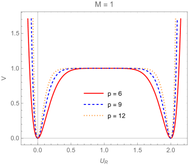
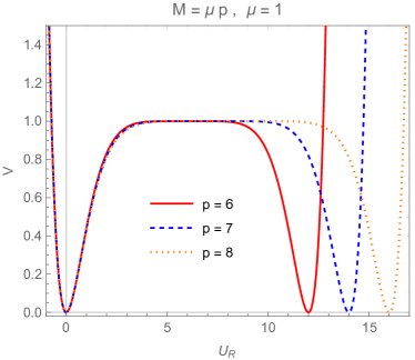
Figure 1: Both panels show the potential of the (22) model for different values of $p$ for $M=1$ and $M=p\,\mu$ (left and right panels respectively), where $M$ and $\mu$ are $p$-independent constants. Inflation takes place around the local maximum of the potential. Right panel: Note how the local maximum is moving towards bigger $u_{R}$ for bigger $p$.

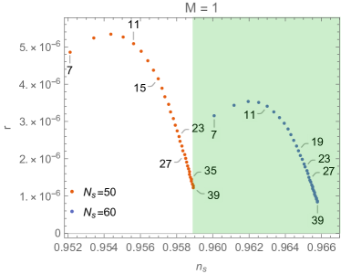
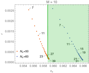
Figure 2: Left Panel: results for the model (22) model for $M=1$, $p\in(7,39)$ and $N_{\star}=50$ and $N_{\star}=60$ (orange and blue dots respectively). Right panel: The same results for $M=10$. Note how the predicted value of $r$ rise up with $M$.

III.3 Generalization of the Starobinsky Inflation

For

$$f(T)=-\frac{M}{\sqrt{2}}\log\left(1-T\right)\,,\qquad w=T\,,$$ (24)

one finds the scalar potential of the form of

$$V=\Lambda^{2}e^{u_{I}^{2}}\left(1-2e^{-\frac{u_{R}}{M}}\cos\left(\frac{u_{I}}{M}\right)+e^{-2\frac{u_{R}}{M}}\right)\,.$$ (25)

The potential obtains its global minimum for $u_{I}=u_{R}=0$, while the inflation happens for $u_{I}=0$ and $u_{R}>M$. In such a case the potential (25) takes the following approximate form

$$V=\Lambda^{2}\left(1-e^{-\frac{u_{R}}{M}}\right)^{2}\,,$$ (26)

which is a simple generalization of Starobinsky inflation. The model has already been investigated in e.g., Kallosh:2014rga ; Kallosh:2013xya and which can be defined by the following Jordan frame action of the scalar-tensor theory

$$S=\int d^{4}x\sqrt{-g}\left(\frac{\varphi}{2}R-\frac{\omega}{\varphi}(\partial\varphi)^{2}-\Lambda^{2}(\varphi-1)^{2}\right)\,,$$ (27)

where $\omega$ and $\Lambda$ are positive constants. Every model within the scalar-tensor theory may be also discussed in the Einstein frame, for which the metric tensor is transformed into $g^{E}_{\mu\nu}=\varphi g_{\mu\nu}$. In the Einstein frame the gravity is minimally coupled to the scalar field $\varphi$. After the field redefinition $\phi=\sqrt{\beta/2}\log(\varphi)$ one obtains the action

$$S=\int d^{4}x\sqrt{-g^{E}}\left(\frac{1}{2}R^{E}-\frac{1}{2}(\partial\phi)^{2}-\Lambda^{2}(1-e^{-\sqrt{2/\beta}\phi})\right)\,.$$ (28)

Clearly, this model is fully consistent with (26).

In the $M\lesssim 1$ limit the results of this model correspond to $\alpha$-attractors, namely

$$r\simeq 8\frac{M^{2}}{N_{\star}^{2}}\,,\qquad n_{s}\simeq 1-\frac{2}{N_{\star}}\,,$$ (29)

while in the $M\gg 1$ limit the model becomes equivalent to the $V\propto\phi^{2}$ inflation, which gives $r=8/N_{\star}$ and $n_{s}=1-2/N_{\star}$. The inflationary potential for different values of $M$ together with the consistency of the model with the data have been presented in Figure 3. In particular, for $M=\sqrt{3/2}$ or $M=\sqrt{\beta/2}$ one recovers Starobinsky inflation or its Brans-Dicke generalization, respectively. $\beta$ in the Brans-Dicke theory is a parameter defined by the properties of kinetic term of the scalaron and not by mass of fields, just like in Tsujikawa:2013ila .

Please note that this model is a certain limit of the (22) scenario. If in (22) one would consider $M=\mu\,p$, then (22) would be equivalent to (26) for $p\to\infty$. In such a case the stationary point moves towards $u_{R}\to\infty$.

A similar model has been investigated in Pinhero:2018xbk , where the authors consider $K=K_{-}$ and $f(T)=\arctan(T)$. In such a case one recovers the scalar potential equivalent to $\alpha$-attractors, which give predictions very similar to the Starobinsky inflation. The (24) model is a good example on how a choice of $K=K_{+}$ may give radically different results. In such a case one finds

$$V=2\Lambda^{2}\left(1-\cos\left(\frac{u_{I}}{M}\right)\right)\,,$$ (30)

which is a well-known potential of natural inflation Adams:1992bn , which, unlike the Starobinsky inflation, is inconsistent with the data Akrami:2018odb .

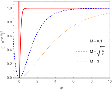
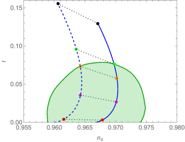
Figure 3: Left panel: Inflationary potential for different values of $M$. For small $M$ the last $60$ e-folds of inflation happens on the plateau, while for $M\gg 1$ the inflationary potential resembles the $V\propto\phi^{2}$ model. Right panel: $r(n_{s})$ for $N_{\star}=50$ and $N_{\star}=60$ (dashed and solid lines respectively). Red, pink, orange and green points corresponds to $M=\sqrt{3/2}$, $M=5$, $M=10$ and $M=50$ respectively. The black points correspond to $r=4(1-n_{s})$, which is the result of the $V\propto\phi^{2}$ model. For $N_{\star}=50$ and $N_{\star}=60$ one obtains the consistency with the data for $M<11$ and $M<17.5$ respectively.

III.4 The Log${}^{2}\phi$ Model for $K=K_{-}$

Following the general model defined in the Section II let us consider the following theory

$$f=\frac{M}{\sqrt{2}}e^{T}\,,\qquad w=T\,,$$ (31)

which from (10) gives the following form of the scalar potential

$$V=\Lambda^{2}e^{u_{I}^{2}}\left(\frac{1}{4}\log^{2}\left(\frac{u_{R}^{2}+u_{I}^{2}}{M^{2}}\right)+\arctan^{2}\left(\frac{u_{I}}{u_{R}}\right)\right)\,.$$ (32)

Inflation takes place in the valley of $u_{I}=0$. Global minima of the potential are $u_{I}=0$ and $u_{R}=\pm M$, for which one finds $V=0$. The potential along the inflationary trajectory reads

$$V(u_{I}=0)=\Lambda^{2}\log^{2}\left(\frac{|u_{R}|}{M}\right)\,.$$ (33)

The entire evolution of the field may be described as reaching the $u_{I}=0$ valley from random initial conditions and then following the valley until $u_{R}$ reach global minimum at $u_{R}=\pm M$. The results for such a model line plotted in Figure 4 (dashed line). Again, we want to emphasize that the $\log^{2}(|u_{R}|/M)$ potential could not be obtained using the standard $K=-\frac{1}{2}(T-\bar{T})^{2}$ from Kallosh:2010xz , since $W\propto\log(T)$ is non-holomorphic.

III.4.1 The $K=K_{+}$ Scenario

This model has this interesting feature, where both $V_{+}$ and $V_{-}$ may generate successful inflation. The scalar potential $V_{+}$ as a function of $u_{R}$ and $u_{I}$ is presented in the Figure 5. In the case of $K=K_{+}$ the evolution of fields may look more complicated. First, the field reaches the $u_{R}=0$ valley, for which the inflationary potential may be approximated as

$$V(u_{R}=0)=\Lambda^{2}\left(\log^{2}\left(\frac{u_{I}}{M}\right)+\left(\frac{\pi}{2}\right)^{2}\right)\,.$$ (34)

Inflation occurs while $|u_{R}|\ll M$ and $u_{I}\gg M$. In addition, in order to enable the inflaton to reach the global minimum at $(u_{I},u_{R})=(0,\pm M)$ one requires $M<M_{c}\equiv\sqrt{e}\simeq 1.65$. Otherwise the inflaton finds itself in a de Sitter (dS) minimum at the end of the logarithmic slope and graceful exit becomes possible only via quantum tunneling. The results of the (34) model for $M=1$ presented in the Figure 4 (solid line). The potentials for both $M<M_{c}$ and $M>M_{c}$ are presented in the Figure 5.

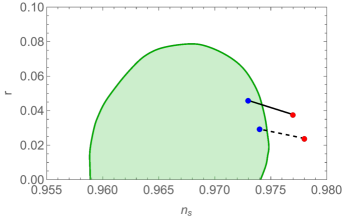
Figure 4: Results for the (33) model for $M=1$. Solid (dashed) lines correspond to $K=K_{+}$ ($K=K_{-}$), while red and blue dots represent $N_{\star}=60$ and $N_{\star}=50$ respectively. The consistency with the data requires $N_{\star}\simeq 50$.

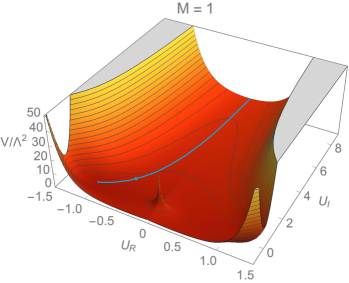
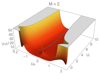
Figure 5: Both panels present scalar potential from Equation (31) with $K=K_{+}$, as a function of $u_{R}$ and $u_{I}$. During inflation $|u_{R}|\ll M\ ,\ |u_{I}|\gg M$ and after inflation the field rolls towards one of the minima at $u_{I}=0$ and $u_{R}=\pm M$ (left panel). For $M>M_{c}$, the field is stuck in the dS vacuum separated from the true vacuum by a local maximum (right panel). Blue lines present the evolution of fields $u_{R}$ and $u_{I}$ from the inflationary plateau to their minima.

In the close vicinity of $M=M_{c}$ one obtains another possibility of inflation along the $u_{R}$ direction. To see that let us investigate the evolution of the field for $u_{I}\ll M$, when inflation along the $u_{I}$ direction is over. In such a case, one finds

$$V\propto e^{u_{R}^{2}}\log^{2}\left(\frac{u_{R}}{M}\right)\,.$$ (35)

As shown in the Figure 6, the potential develops a local minimum for $M>M_{c}$, which prevents the field to reach its global minimum. For $M\leq M_{c}$ the only existing minima are in $u_{R}=\pm M$. For $M=M_{c}$ one obtains a saddle point at $u_{R}=1$, which means that inflation has two phases. The first one happens at the logarithmic slope of the $\log^{2}(u_{I})$ inflation, while the second one happens at the plateau in the vicinity of $u_{R}\simeq\sqrt{2}$.

The inflation along the $u_{R}$ direction requires certain fine-tuning. To obtain at least 60 e-folds one requires $M_{c}-M\lesssim\mathcal{O}(10^{-4})$. In addition, as shown in the Figure 6, the consistency with the data requires $M_{c}-M\simeq 10^{-5}M_{c}$. The reason for the fine-tuning is the following—for the saddle-point inflation one obtains $n_{s}\simeq 0.92$, which is highly inconsistent with Planck/BICEP data. Thus, one must deviate from the saddle-point scenario and assume an inflection-point potential. On the other hand, the plateau obtained in this model is quite short, so even small deviations from the saddle-point inflation lead to insufficient number of e-folds.

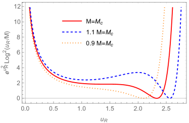
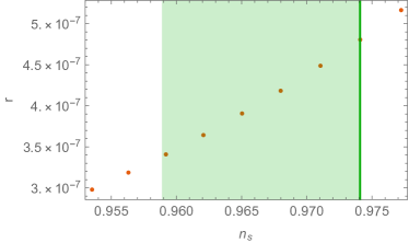
Figure 6: Left panel: The potential (35) for $M\simeq M_{c}$. For $M=M_{c}$ one obtains a saddle point, around which one obtains a second phase of inflation. For $M>M_{c}$ one obtains a local maximum, which separates the inflaton from the Minkowski vacuum. Right panel: results for the (35) on the $(n_{s},r)$ plane. Dots correspond to $M=(1-k\times 5\times 10^{-6})M_{c}$, where $k\in\{12,13,\ldots,20\}$ and bigger $k$ corresponds to bigger $n_{s}$. Inflation can be only consistent with the data for $(1-9.5\times 10^{-5})M_{c}\lesssim M\lesssim(1-7\times 10^{-5})M_{c}$, which means that the model requires significant fine-tuning in order to be within the $2\sigma$ regime of Planck/BICEP results.

III.5 a Simple Plateau Model

One may easily obtain a flat inflationary potential using the following field redefinition and superpotential

$$f=\frac{1}{\sqrt{2}}\frac{1}{T}\,,\qquad w=T-1\,.$$ (36)

In such a case the potential is equal to

$$V=\Lambda^{2}e^{2u_{I}^{2}}\left(\left(u_{I}^{2}+u_{R}^{2}\right)^{-1}-2\left(u_{I}^{2}+u_{R}^{2}\right)^{-\frac{1}{2}}\cos\left(\arctan\left(\frac{u_{I}}{u_{R}}\right)\right)+1\right)\,.$$ (37)

Inflation happens in the $u_{I}=0$ valley, which leads to simple inflationary potential of the form of

$$V(u_{I}=0)=\Lambda^{2}\left(1-\frac{1}{u_{R}}\right)^{2}\,.$$ (38)

In such a case one finds the global minimum of the potential at $u_{R}=\pm 1$ and $u_{I}=0$. The scalar potential (38) is presented in Figure 7. The model can be easily generalized into $f(T)=\frac{1}{\sqrt{2}}T^{-n}$, which gives $V=\Lambda^{2}(1-u_{R}^{-1})^{2n}$. Increasing $n$ decreases $r$ and moves $n_{s}$ inside the $2\sigma$ of the Planck/BICEP data. The results for $n=1$, $n=2$ and $n=4$ are presented in the Figure 7. Please note that the same model could be obtained using different $f(T)$ and $w(T)$. For instance, for $f=e^{T}/\sqrt{2}$ and string-inspired superpotential $w=e^{-T}-1$ one obtains exactly the same form of $V(U)$.

As in the case of Starobinsky inflation, this model could easily be embedded in a scalar-tensor theory. The Jordan frame action

$$S=\int d^{4}\sqrt{-g}\left(\frac{\varphi}{2}R-\frac{\omega}{\varphi}(\partial\varphi)^{2}-\lambda^{2}\varphi^{2}\left(1-\frac{\sqrt{2/\beta}}{\log\varphi}\right)^{2}\right)$$ (39)

can be transformed to the Einstein frame action and potential by a standard field redefinition. This Einstein frame potential will be fully consistent with (38).

Both spectral index and tensor-to-scalar ratio can be found analytically. Using the $N_{\star}\gg 1$ approximation one finds $u_{R\star}=u_{R}(N_{\star})\simeq(2n(n+2)N_{\star})^{\frac{1}{n+2}}$, which gives

$$r\simeq\frac{2^{5}n^{2}}{(2n(n+2)N_{\star})^{\frac{2(n+1)}{n+2}}}\,,\qquad n_{s}\simeq 1-\frac{12n^{2}}{(2n(n+2)N_{\star})^{\frac{2(n+1)}{n+2}}}-\frac{2(n+1)}{(n+2)N_{\star}}\,.$$ (40)

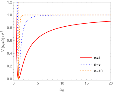
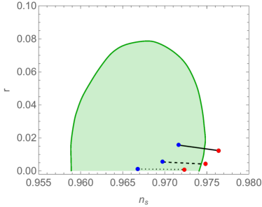
Figure 7: Left panel: The inflationary potential of model (36) and its generalization $V=\Lambda^{2}(1-u_{R}^{-1})^{2n}$. Right panel: The tensor-to-scalar ratio and the spectral index for $N_{\star}=50$ and $N_{\star}=60$ (solid line, blue and red dots respectively). Dashed and dotted lines represent results for the generalization of the model, for which one has taken $f(T)=T^{-n}/\sqrt{2}$. Solid, dashed and dotted lines correspond to $n=1$, $n=2$ and $n=4$ respectively.

III.6 Plateau from the Modular Transformation

Let us return to $w=T$, but with

$$f=\frac{aT+b}{cT+d}\,.$$ (41)

This form of $f(T)$ can be motivated by the modular transformation, for which $ad-bc=1$. For the modular transformation one requires $a,b,c$ and $d$ to be integers. One can also consider more generic case of the $PSL(2,\mathbb{R})$ group, for which one finds $a,b,c,d\in\mathbb{R}$.

For $K=K_{-}$ and $u_{I}=0$ one finds

$$V=\Lambda^{2}\left(\frac{\sqrt{2}b-d\,u_{R}}{\sqrt{2}a-c\,u_{R}}\right)^{2}\,.$$ (42)

One can simplify this potential using $ad-bc=1$ and a simple field transformation $u_{R}\to u_{R}+\sqrt{2}a/c$, which gives

$$V=\Lambda^{2}\frac{d^{2}}{c^{2}}\left(1+\frac{\sqrt{2}}{c\,d}\frac{1}{u_{R}}\right)^{2}\,.$$ (43)

The (43) model is simply a generalization of the (38).

On the other hand, for $K=K_{+}$ one finds

$$V(u_{R}=0)=\Lambda^{2}\frac{2b^{2}+d^{2}u_{I}^{2}}{2a^{2}+c^{2}u_{I}^{2}}\,.$$ (44)

This potential obtains a minimum for $u_{I}=0$. To obtain a Minkowski vacuum one requires $b=0$, which together with $ad-bc=1$ gives

$$V=\frac{\Lambda^{2}}{a^{4}}\frac{\phi^{2}}{2+\left(\frac{c}{a}\right)^{2}\phi^{2}}\,.$$ (45)

The $a^{4}$ term is a part of the normalization of the potential, which could be absorbed into $\Lambda$ and does not affect $r$ and $n_{s}$. Thus, from the point of view of the predictions on the $(n_{s},r)$ plane, the model has only one parameter, which is $c/a$. The (45) potential has two limits. For $\phi^{2}\ll a^{2}/c^{2}$ one finds $V\propto\phi^{2}$, while for $\phi^{2}\gg a^{2}/c^{2}$ the potential obtains inflationary plateau. The potential for the (45) model is shown in the Figure 8. Assuming the slow-roll approximation one finds

$$r \simeq \frac{16}{\left(\frac{a^{2}}{c^{2}}+4N_{\star}\right)\left(\sqrt{\frac{4c^{2}N_{\star}}{a^{2}}+1}-1\right)}\,,$$

$$n_{s} \simeq 1-\frac{1}{N_{\star}}\left(\frac{1}{\sqrt{\frac{4c^{2}N_{\star}}{a^{2}}+1}}+1\right)-\frac{2}{\frac{a^{2}}{c^{2}}+4N_{\star}}\,.$$ (46)

In the small/big $4N_{\star}c^{2}/a^{2}$ limit $r$ and $n_{s}$ can be further simplified to

$$r\simeq\left|\frac{a}{c}\right|\frac{2}{N_{\star}^{3/2}}\,,\qquad n_{s}\simeq 1-\frac{3}{2N_{\star}}\qquad \qquad 4N_{\star}c^{2}/a^{2}\gg 1\,,$$ for (47)

$$r\simeq\frac{8}{N_{\star}}\,,\qquad n_{s}\simeq 1-\frac{2}{N_{\star}}\qquad \qquad 4N_{\star}c^{2}/a^{2}\ll 1\,.$$ for (48)

In the $4N_{\star}c^{2}/a^{2}\ll 1$ one finds $r\sim 10^{-1}$, which is inconsistent with PLANCK/Bicep data. The comparison to the Planck/BICEP data is presented in Figure 9.

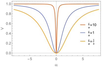
Figure 8: Potential (45) for different values of $c/a$. Please note that for $c\gg a$ , inflation takes place predominantly at the plateau, while for $c\ll a$ the last 60 e-folds of inflation happen around the $\phi^{2}$ slope.

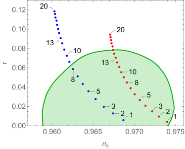
Figure 9: Results for the (45) model for both $c/a>1$ and $c/a<1$. Blue and red dots represent $N=50$ and $N=60$ respectively. Left panel: We consider $k=c/a$ and $k\in\{1,2,\ldots,10\}$. Right panel: $k=a/c$ and $k\in\{1,2,\ldots,20\}$. Note how in the $c\ll a$ limit one moves towards the results of $\phi^{2}$ inflation.

III.7 Bell-Curve Potentials

Let us consider

$$f=-\frac{1}{\sqrt{2}}M\log^{p}(T)\,,\qquad w=T\,,$$ (49)

which gives the scalar potential of the form of

$$V=\Lambda^{2}\exp\left(u_{I}^{2}-2\left(\frac{u_{R}^{2}+u_{I}^{2}}{M^{2}}\right)^{\frac{1}{2p}}\cos\left(\frac{1}{p}\arctan\frac{u_{I}}{u_{R}}\right)\right)\,.$$ (50)

Inflation happens for $u_{I}=0$, which for a generic value of $p$ gives the following inflationary potential

$$V(u_{I}=0)=\Lambda^{2}\exp\left(-\left|\frac{u_{R}}{M}\right|^{1/p}\right)\,.$$ (51)

The shape of the potential for $p>0$ and $p<0$ is presented in the Figure 10. This model could also be expressed using a string-inspired superpotential $w=e^{-T}$ together with $f=MT^{p}/\sqrt{2}$. Within the slow-roll approximation one finds

$$r \simeq 16\left(\frac{2N_{\star}(1-2p)}{\left(\sqrt{2}M|p|\right)^{\frac{1}{1-p}}}+1\right)^{-\frac{2(1-p)}{1-2p}}\,$$ (52)

$$n_{s} \simeq 1-2\left(\frac{2N_{\star}(1-2p)}{\left(\sqrt{2}M|p|\right)^{\frac{1}{1-p}}}+1\right)^{-\frac{2(1-p)}{1-2p}}-\frac{4(1-p)}{\left(\sqrt{2}M|p|\right)^{\frac{1}{1-p}}+2N_{\star}(1-2p)}\,.$$ (53)

Please note that in the

$$N_{\star}\ll\frac{1}{2(1-2p)}\left(\sqrt{2}M|p|\right)^{\frac{1}{1-p}}$$ (54)

regime equation (52) takes the form of

$$\epsilon\simeq\frac{\epsilon_{0}}{N^{n}}\,,$$ (55)

where $M=(2p-1)\sqrt{\epsilon_{0}}(2(1-2p)\epsilon_{0})^{-p}p^{-1}$ and $n=2(p-1)/(2p-1)$. $0<p<1/2$ corresponds to $n>2$, while $p<0$ to $1<n<2$. Please note that the $p\to 0$ limit corresponds to $\epsilon\propto N^{-2}$, which is the feature of theories like Starobinsky inflation, Higgs inflation, or $\alpha$-attractors. Indeed, for $|p|M\ll 1$ one finds

$$r\simeq 8\frac{M^{2}p^{2}}{N_{\star}^{2}}\,,\qquad n_{s}\simeq 1-\frac{2}{N_{\star}}\,,$$ (56)

which is the result of the (26) model for $M\to M|p|$.

The (55) parametrization is widely used in cosmology (see e.g., Mukhanov:2014uwa ), which is an additional motivation to consider this model. We have assumed $n\neq 1$ and $n\neq 2$, since $n=1$ or $n=2$ correspond to well-known cases of the power-law and Starobinsky potentials, respectively. One can strongly constrain the possible range of $n$ (and consequently, the range of $p$) using the Planck/BICEP data. Since $\frac{dN}{d\phi}=1/\sqrt{2\epsilon}$, one finds

$$\frac{d\sqrt{2\epsilon}}{d\phi}=\pm\frac{1}{\sqrt{2\epsilon}}\frac{d\sqrt{2\epsilon}}{dN}=\pm\frac{\epsilon_{N}}{2\epsilon}\,,$$ (57)

as well as

$$\frac{d\sqrt{2\epsilon}}{d\phi}=\pm\frac{d}{d\phi}\frac{V_{\phi}}{V}=\pm\left(\eta-2\epsilon\right)\,,$$ (58)

where $\epsilon_{N}=\frac{d\epsilon}{dN}$. Therefore, one can express $\eta$ as

$$\eta=2\epsilon+\frac{\epsilon_{N}}{2\epsilon}\,,\qquad n_{s}=1-6\epsilon+2\eta=1+\frac{\epsilon_{N}}{2\epsilon}-2\epsilon\,.$$ (59)

Using the (55) one finds

$$\eta=2\frac{\epsilon_{0}}{N^{n}}\,,\qquad n_{s}=1-\frac{n}{N}-2\frac{\epsilon_{0}}{N^{n}}\,.$$ (60)

Since we require $n_{s}$ to be in the vicinity of $0.96$ one cannot obtain a result consistent with Planck/BICEP data for $n$ significantly bigger than 2. The results for the (51) model are presented in Figure 11.

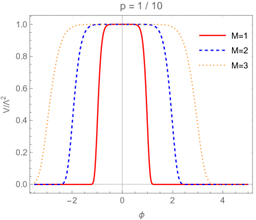
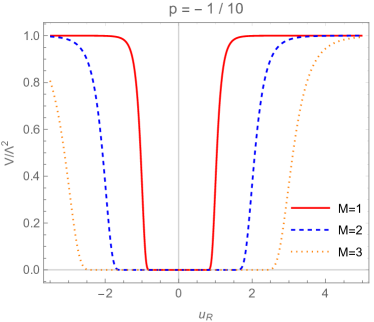
Figure 10: Potential (51) for $p>0$ and $p<0$ (left and right panel respectively). For $p>0$ inflation happens around the local maximum and the potential does not have a minimum. For $p<0$ inflation happens on one of the infinite plateaus separated by the minimum.

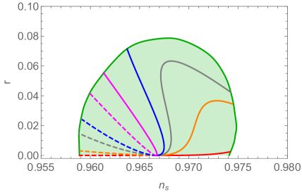
Figure 11: Results for the (51) model for $N_{\star}=60$ and $p<0$ or $p>0$ (solid and dashed lines respectively). Red, orange, gray, blue and pink lines represent $M=1$, $M=10$, $M=20$, $M=30$ and $M=100$ and $p\in(-0.44,0.16)$, $p\in(-1.3,0.152)$, $p\in(-1.7,0.132)$, $p\in(-0.28,0.106)$ and $p\in(-0.053,0.042)$ respectively. Note how results for different $M$ reproduce the result of the Starobinsky inflation in the $p\to 0$ limit. In addition, the results of the (51) model may cover the whole $2\sigma$ regime of the Planck/BICEP data.

Let us discuss possible reheating mechanisms in this scenario. In general, for any $p$ reheating may happen at the post-inflationary slope, e.g., via instant preheating Felder:1998vq and for $p<0$ through the standard reheating oscillations. However, in our case we have a built-in gravitational particle production Ford:1986sy ; Artymowski:2017pua for any $p$ if our inflaton is of the dark sector. This is due to the steepness of the post-inflationary potential. In the gravitational reheating case the post-inflationary evolution is dominated by the inflaton with an equation of state $w=1$. Reheating (understood as the beginning of the radiation domination) happens around $T_{R}\sim\mathcal{O}(10^{7}GeV)$. Hence, this is another prediction of the model, which narrows down possible values of $N_{\star}$ and $n_{s}$.

To conclude, the (51) model has several interesting features, which are worth exploring in detail. The model spans the entire allowed $(n_{s},r)$ region, which makes its predictions consistent with any future experiment that would constrain these parameters. This means that inflation can have an arbitrarily low scale, which is strongly favored by the trans-Planckian censorship conjecture Brahma:2019vpl ; Cai:2019dzj ; Berera:2020dvn . The model also contains an inflationary attractor in the $p\to 0$ limit, which is Starobinsky-like. In addition, the model has a built-in predictive mechanism of gravitational reheating, due to the post-inflationary kination of the inflaton. Thus, one does not require any additional assumptions regarding the couplings of the inflaton to matter fields.

IV Conclusions

The main idea of this paper is to show that assuming a particular flat Kähler potential $K_{\pm}=\pm\frac{1}{2}(T\pm\bar{T})^{2}+S\bar{S}$ and a specific superpotential $W=\Lambda S\,T$ one can obtain a wide spectrum of inflationary theories differentiated only by a field redefinition applied solely to the Kähler potential $K(f(T),\bar{f}(\bar{T}),S\bar{S})$ as introduced in Section II. A canonical Kähler potential may be restored after the field redefinition $U=f(T)$. Following this transformation of the Kähler potential, a generic form of a scalar potential has been obtained, while the Kähler geometry remained flat.

In a few simple examples, we have demonstrated completely different classes of models, small field, Starobinsky, large field and even a squared logarithmic potential as suggested in Ben-Dayan:2018mhe . In Sections III.1–III.3 we have presented the results of well-known inflationary models. Our goal is to emphasize that one can obtain them in a novel way using a flat Kähler geometry and a simple fixed superpotential $W=\Lambda\,S\,T$. We have also constructed the plateau model from a modular or PSL(2,R) transformation that covers most of the allowed parameter space. The predictions of investigated models span $r\in[10^{-6},0.06]$, and a valid $n_{s}$ for reasonable number of e-folds. Of particular interest are the bell-curve models since their predictions cover all allowed values of $r$ and $n_{s}$. In addition, due to the kination of the inflaton after inflation, the model has a built-in predictive mechanism of gravitational reheating, which does not require additional couplings of $T$ to matter fields. The specific details of the analyzed models are given in Section III.

The idea of the field redefinition bypasses the limit of holomorphicity used for generating general potentials by having an arbitrary holomorphic function $f(T)$ in $W$. This is because at the fundamental level, with the $T$ field, we have the same holomorphic $W$, and what one really has are different real Kahler potentials, but all with the same Kahler geometry. As such, the construction abides the standard rules of SUGRA models. We have focused on the F-term scalar potential in SUGRA. It would be interesting to apply this method for D-term inflationary model building as well.

References

- (1) Starobinsky, A.A. A New Type of Isotropic Cosmological Models Without Singularity. Phys. Lett. 1980, 91, 99.
- (2) Lyth, D.H.; Riotto, A. Particle physics models of inflation and the cosmological density perturbation. Phys. Rep. 1999, 314, 1.
- (3) Sato, K. First Order Phase Transition of a Vacuum and Expansion of the Universe. Mon. Not. Roy. Astron. Soc. 1981, 195, 467.
- (4) Guth, A.H. The Inflationary Universe: A Possible Solution to the Horizon and Flatness Problems. Phys. Rev. D 1981, 23, 347.
- (5) Akrami, Y.; Arroja, F.; Ashdown, M.; Aumont, J.; Baccigalupi, C.; Ballardini, M.; Banday, A.J.; Barreiro, R.B.; Bartolo, N.; Basak, S.; et al. Planck 2018 results. X. Constraints on inflation. arXiv 2018, arXiv:1807.06211.
- (6) Kallosh, R.; Linde, A.; Roest, D. Superconformal Inflationary -Attractors. JHEP 2013, 1311, 198, doi:10.1007/JHEP11(2013)198.
- (7) Artymowski, M.; Rubio, J. Endlessly flat scalar potentials and -attractors. Phys. Lett. B 2016, 761, 111, doi:10.1016/j.physletb.2016.08.024.
- (8) Dimopoulos, K.; Artymowski, M. Initial conditions for inflation. Astropart. Phys. 2017, 94, 11, doi:10.1016/j.astropartphys.2017.06.006.
- (9) Kawasaki, M.; Yamaguchi, M.; Yanagida, T. Natural chaotic inflation in supergravity. Phys. Rev. Lett. 2000, 85, 3572.
- (10) Ben-Dayan, I.; Einhorn, M.B. Supergravity Higgs Inflation and Shift Symmetry in Electroweak Theory. JCAP 2010, 1012, 2.
- (11) Nakayama, K.; Takahashi, F. Higgs Chaotic Inflation in Standard Model and NMSSM. JCAP 2011, 1102, 10.
- (12) Badziak, M.; Olechowski, M. Volume modulus inflation and a low scale of SUSY breaking. JCAP 2008, 807, 21.
- (13) Ben-Dayan, I.; Brustein, R.; de Alwis, S.P. Models of Modular Inflation and Their Phenomenological Consequences. JCAP 2008, 807, 11.
- (14) Covi, L.; Gomez-Reino, M.; Gross, C.; Louis, J.; Palma, G.A.; Scrucca, C.A. Constraints on modular inflation in supergravity and string theory. JHEP 2008, 808, 55.
- (15) Kallosh, R.; Linde, A.; Rube, T. General inflaton potentials in supergravity. Phys. Rev. D 2011, 83, 43507.
- (16) Volovik, G.; Zubkov, M. Emergent Weyl spinors in multi-fermion systems. Nucl. Phys. B 2014, 881, 514–538.
- (17) Gorbar, E.; Miransky, V.; Shovkovy, I. Chiral anomaly, dimensional reduction, and magnetoresistivity of Weyl and Dirac semimetals. Phys. Rev. B 2014, 89, 85126.
- (18) Parrikar, O.; Hughes, T.L.; Leigh, R.G. Torsion, Parity-odd Response and Anomalies in Topological States. Phys. Rev. D 2014, 90, 105004.
- (19) Horava, P. Stability of Fermi surfaces and K-theory. Phys. Rev. Lett. 2005, 95, 16405.
- (20) Volovik, G. The Universe in a helium droplet. Int. Ser. Monogr. Phys. 2006, 117, 1–526.
- (21) Galante, M.; Kallosh, R.; Linde, A.; Roest, D. Unity of Cosmological Inflation Attractors. Phys. Rev. Lett. 2015, 114, 141302.
- (22) Dalianis, I.; Watanabe, Y. Probing the BSM physics with CMB precision cosmology: An application to supersymmetry. JHEP 2018, 2, 118.
- (23) Boubekeur, L.; Lyth, D.H. Hilltop inflation. JCAP 2005, 507, 10.
- (24) Ben-Dayan, I.; Jing, S.; Westphal, A.; Wieck, C. Accidental inflation from Kähler uplifting. JCAP 2014, 1403, 54.
- (25) Ben-Dayan, I.; Brustein, R. Cosmic Microwave Background Observables of Small Field Models of Inflation. JCAP 2010, 1009, 7.
- (26) Pinhero, T.; Pal, S. Realising Mutated Hilltop Inflation in Supergravity. Phys. Lett. B 2019, 796, 220.
- (27) Hamada, Y.; Kawai, H.; Kawana, K. Saddle point inflation in string-inspired theory. PTEP 2015, 2015, 91B01.
- (28) Kallosh, R.; Linde, A.; Roest, D. Large field inflation and double -attractors. JHEP 2014, 1408, 52.
- (29) Kallosh, R.; Linde, A. Superconformal generalizations of the Starobinsky model. JCAP 2013, 1306, 28.
- (30) Tsujikawa, S.; Ohashi, J.; Kuroyanagi, S.; Felice, A.D. Planck constraints on single-field inflation. Phys. Rev. D 2013, 88, 23529.
- (31) Pinhero, T. Natural -Attractors from Supergravity via flat Kähler Manifolds. arXiv 2018, arXiv:1812.05406.
- (32) Adams, F.C.; Bond, J.R.; Freese, K.; Frieman, J.A.; Olinto, A.V. Natural inflation: Particle physics models, power law spectra for large scale structure, and constraints from COBE. Phys. Rev. D 1993, 47, 426.
- (33) Mukhanov, V. Inflation without Selfreproduction. Fortsch. Phys. 2015, 63, 36.
- (34) Felder, G.N.; Kofman, L.; Linde, A.D. Instant preheating. Phys. Rev. D 1999, 59, 123523.
- (35) Ford, L.H. Gravitational Particle Creation and Inflation. Phys. Rev. D 1987, 35, 2955.
- (36) Artymowski, M.; Czerwinska, O.; Lalak, Z.; Lewicki, M. Gravitational wave signals and cosmological consequences of gravitational reheating. JCAP 2018, 1804, 46.
- (37) Berera, A.; Brahma, S.; CalderĂłn, J.R. Role of trans-Planckian modes in cosmology. arXiv 2003, arXiv:2003.07184.
- (38) Brahma, S. Trans-Planckian censorship conjecture from the swampland distance conjecture. Phys. Rev. D 2020, 101, 46013.
- (39) Cai, R.; Wang, S. A refined trans-Planckian censorship conjecture. arXiv 2019, arXiv:1912.00607.
- (40) Ben-Dayan, I. Draining the Swampland. Phys. Rev. D 2019, 99, 101301.