Salient Speech Representations Based on Cloned Networks

Abstract

We define salient features as features that are shared by signals that are defined as being equivalent by a system designer. The definition allows the designer to contribute qualitative information. We aim to find salient features that are useful as conditioning for generative networks. We extract salient features by jointly training a set of clones of an encoder network. Each network clone receives as input a different signal from a set of equivalent signals. The objective function encourages the network clones to map their input into a set of features that is identical across the clones. It additionally encourages feature independence and, optionally, reconstruction of a desired target signal by a decoder. As an application, we train a system that extracts a time-sequence of feature vectors of speech and uses it as a conditioning of a WaveNet generative system, facilitating both coding and enhancement.

Index Terms: Features, representation, speech, Siamese network, generative network, maximum mean discrepancy.

1 Introduction

In speech processing, as well as other applications, it is valuable to find a meaningful representation that summarizes the salient attributes of a signal. We define a salient feature set as a feature set that is shared by signals that are judged to be equivalent by a user. This definition allows the user to contribute qualitative knowledge to a feature extraction procedure, a weak form of supervision. We aim to use this paradigm to extract feature sets that can be used as conditioning for generative networks. A successful salient feature set can be used for the storage or transmission of signals, or for the manipulation of signal attributes. Examples are the robust coding of speech, changing the identity of a talker, and resynthesizing a speech signal without noise.

Autoencoders provide perhaps the most natural approach towards finding a meaningful representation, although other approaches such as generative adversarial networks can also be used, e.g., [1]. Autoencoders map an input signal to a set of latent variables, the representation, with an encoder and map the latent variables to the output with a decoder. In recent years, research has focused on various forms of the variational autoencoder (VAE) [2, 3]. The primary goal of the original VAE was to create a generative system (the decoder) and the encoder arose from the need for a practical training algorithm. Because the encoder has a stochastic nature, the latent representation is expected to have a smooth relation with the input. The original VAE formulation was found to ignore the input in many cases, making the latent representation not meaningful. Numerous methods have been proposed to address this problem, referred to as information preference property or posterior collapse, e.g., [4, 5, 6, 7, 8, 9].

In addition to signal features varying smoothly over the latent support space, it is desirable that these features are disentangled. In disentangled representations, different latent dimensions exclusively control different factors of variation of the data (e.g., location, orientation) [10, 11]. $\beta$-VAE [12] re-weights the components of the VAE objective function, which encourages disentanglement at the cost of a lower reconstruction accuracy [13, 14, 15]. $\beta$-VAE can be interpreted [13] as approximation to the information bottleneck (IB) [16] and hence is related to [17]. Other approaches explicitly encourage independence by means of maximum mean discrepancy [11] and, recently, by means of total correlation (the Kulback-Leibler divergence between the joint distribution and the product of the marginal distributions) [15].

Conventional VAEs are not aware of saliency as we defined it. VAEs commonly use a maximum-likelihood objective combined with a Gaussian assumption for reconstruction accuracy, which is equivalent to a straight squared error criterion. The network is not informed about the perceptual importance of features to a user. Hence, a VAE-based representation may include features that are perceptually irrelevant but require a significant rate allocation. Indeed,[18] shows that most information about the signal waveform is perceptually not relevant.

Salient information has been separated in VAEs using semi-supervised learning that separates out nuisance variables and class information from the latent representation [11]. This approach requires explicit knowledge of these variables for at least part of the database.

The IB method suggests a method for extracting features that are salient based on our definition. The IB finds a representation that is maximally informative about a target output, given a bound on the information available about the input. The approach was illustrated with a sequence of phonemes as target output [19]. By training a network to extract features from a signal that are maximally informative about an equivalent signal, salient features can be extracted. However, only pairs of equivalent signals can be used for each training instance.

Our contribution is a method to extract from a signal a sequence of salient feature vectors. It is based on the Siamese network structure [20, 21, 22], but can be endowed with a decoder. During training, clones of an encoder network with identical weights are encouraged to map equivalent signals to shared feature vectors. Our objective function encourages i) that the feature vectors are identical across the clones, ii) that the features are independent, iii) optionally, that the feature set can be mapped to a shared target signal.

We applied the new method to the extraction of robust features for speech coding and enhancement. As equivalent signals we used various distorted speech signals and for the optional decoder we use a clean signal as target. Including a target signal enhances the clarity of the linguistic meaning of an already natural-sounding signal. Experiments with WaveNet [23] confirmed that the resulting feature set performs significantly better in terms of robustness to noise than a conventional feature set.

2 Extracting Salient Features

In this section we first motivate and describe the basic extraction network in 2.1. We then describe clone-based training procedures for the method in 2.2. We denote random variables (RVs) with upper case and realizations with lower case font.

2.1 The encoder network

Our objective is to extract salient representations that can be used as conditioning for generative models of speech. As noted in section 1, we define salient features as features that are shared between signals that are deemed equivalent by users. From each signal within a set of equivalent signals, the encoder should extract feature sequences with numerically similar values.

The encoder is a map from an input vector $x$ to a salient feature vector $z$. A sequence is obtained by repeating this process. For a meaningful feature vector $z$, we desire the map to have three basic attributes:

1. Signals that are equivalent result in (almost) identical features.

2. The map is smooth. Different regions of feature space can be identified with different signal attributes, rendering the representation meaningful.

3. The components have a prescribed variance and are independent. Ideally they are distentangled: the system then discovers a ’natural’ set of independent features corresponding to ground-truth factors [10].

The first desired attribute requires a surjective mapping from the speech signal to a salient feature set. We show it can be obtained by training clones of a network with identical weights to output the same features for equivalent signals.

The second desired attribute can be obtained with various strategies. A first approach is to simply restrict the mapping to be smooth deterministic (e.g., Lipschitz smooth). A second approach is to use a stochastic map during training. To see this, consider a feature variable of the form $Z=f(X)+\epsilon$, where $f(\cdot)$ is a deterministic map and $\epsilon\sim p_{\epsilon}$. Then $Z$ is more informative about the input $X$ if the map $f(\cdot)$ is smooth. Such a probabilistic-mapping approach to obtaining a meaningful representation is employed by VAEs, e.g., [2, 3, 9] and this proven strategy will be employed here, also because it aids with the third attribute. While the probabilistic mapping is used to encourage smoothness of the mapping during training, it can be removed in the final deployment of the resulting system for enhanced fidelity. Then, the mapping from speech to features is deterministic at inference.

The third desired attribute of the map facilitates interpretation, coding, and manipulation. Distentanglement of the ground-truth factors is challenging, as a mapping from speech to salient features can map a continuously distributed random speecph vector into a random feature vector with any desired distribution. Without loss of generality, let us consider unit-variance factors. Separation of these factors becomes tractable in the context of equivalent signals, since their variance across an equivalent signal set is, in general, distinct from each other. Hence a ’natural’ set of features can be discovered.

We implement the probabilistic encoder as follows. Let $\phi$ describe the parameter set of the encoder network. We then construct a network of the form

$$z =g_{\phi}(u,\epsilon)$$ (1)

$$u =f_{\phi}(x),$$ (2)

where $f_{\phi}$ and $g_{\phi}$ are surjective mappings, $\epsilon$ is noise drawn from a prescribed probability distribution, $u$ is a vector, and $z$ is the feature vector. In practice we use the following simple and natural realization of the arrangement:

$$z =f_{\phi}(x)+\sigma_{\epsilon}\epsilon,$$ (3)

where $\epsilon\sim\mathcal{N}(0,I)$ is drawn from a zero-mean multivariate normal distribution, with identity as covariance matrix, and $\sigma_{\epsilon}$ is a gain. The map $f_{\phi}(\cdot)$ is implemented with a deep neural network, with its weights characterized by $\phi$. For inference, $\sigma_{\epsilon}$ is set to zero.

2.2 Clone-based training

To allow the encoder network to learn about saliency, we employ clone-based training, which is based on the Siamese network [20] paradigm, but may be endowed with a decoder. A diagram of the method is shown in Fig. 1. Each clone is an identical copy of a basic network. The clones are provided with different input signals that are selected from a set of equivalent signals. The clone-based training structure is used to find what information is shared between the different equivalent signals and to represent that information in the form of features.

To obtain an encoder with the attributes given in section 2.1, we use an objective function with two or three components for clone-based training. A first component encourages the similarity of the feature vectors $z^{(q)}\in\mathbb{R}^{d}$ across the clones $q\in\{1,\cdots,Q\}$. A second component encourages that the distribution of the feature vector is of a desired character. The optional third component encourages the representation to provide high-fidelity decoding to a target signal, which typically is derived from a clean signal.

Let $p_{Z^{(q)}}$ be the probability density of the random feature vector $Z^{(q)}$ with realization $z^{(q)}$ and let $p_{Z^{(1)},\cdots,Z^{(Q)}}$ be the joint density of the feature vectors of the clones. Let $\mathrm{E}[\cdot]$ denote expectation over the input data distribution, which can be approximated by suitable averaging over minibatches. The global objective function is then

$$D(p_{Z^{(1)},\cdots,Z^{(Q)}})=\mathrm{E}[D_{s}(Z^{(1)},\cdots,Z^{(Q)})]+\\ \sum_{i=1}^{Q}\left(\lambda_{f}D_{f}(p_{Z^{(i)}})+\lambda_{d}\mathrm{E}[D_{d}(h_{\psi}(Z^{(i)}),Y)]\right),$$ (4)

where $D_{s}$ is a similarity measure for the clone feature sets, $D_{f}$ is a measure on a distribution, $D_{d}$ is the optional measure of decoder performance, $h_{\psi}$ is the decoder network with trained parameters $\psi$, $Y$ is the desired output, and the $\lambda_{f}$ and $\lambda_{d}$ are weightings. Note that the evaluation of $D_{f}$ and $D_{d}$ can be limited to a smaller number of clones. Below, we discuss the individual terms of the objective function in more detail.

A natural implementation of the first term of (4) is

$$D_{s}(z^{(1)},\cdots,z^{(Q)})=\sum_{q=1}^{Q}\|z^{(1)}-z^{(q)}\|^{2}_{2}.$$ (5)

An alternative is the 1-norm and we can add cross terms for all clones. The shared features are found by encouraging the deterministic mapping $f_{\phi}$ to result in outputs that are maximally similar for all clones, despite their different inputs. The method preferably selects features describing information components that are shared between the clone inputs at relatively high fidelity. For example, if the clones receive noisy versions of segments of a speech signal, then a first feature may describe a measure of spectral amplitude for a frequency region where the signal-to-noise ratio is high. Note that this process naturally leads to disentanglement.

Various approaches can be used to encourage the features to be independent, and have a given variance, some requiring a desired distribution. Examples are the chi-square test, maximum mean discrepancy (MMD) [24, 25], and the earth-moving distance reformulated via the Kantorovich-Rubinstein duality, e.g., [26, 27]. Anticipating sparse features, we implement our system using MMD with an iid Laplacian desired distribution.

Let the desired iid Laplacian distribution be denoted as $p_{\mathcal{D}}$. Let the variable $\mathtt{V}$ be distributed as $\mathtt{V}\sim p_{\mathcal{D}}$. We use as measure on the distribution $p_{p_{Z}^{(1)}}$ the MMD between the distributions $p_{Z^{(1)}}$ and $p_{\mathcal{D}}$:

$$D_{f}(p_{Z^{(1)}})=\mathrm{MMD}(p_{Z^{(1)}},p_{\mathcal{D}})\\ =\sup_{\omega\in\mathcal{H},\,\,\|\omega\|_{\mathcal{H}}\leq 1}\mathrm{E}_{p_{Z^{(1)}}}(\omega(Z^{(1)}))-\mathrm{E}_{p_{\mathcal{D}}}(\omega(\mathtt{V})),$$ (6)

where $\mathcal{H}$ is a selected reproducing kernel Hilbert space (RKHS) and $\omega:\mathbb{R}^{d}\rightarrow\mathbb{R}$ is a witness function that is selected to maximize the discrepancy subject to being in the unit ball in the RKHS. For a RKHS associated with a kernel $k(\cdot,\cdot)$ an empirical representation of the square of (6) is [24, 25]

$$\mathrm{MMD}^{2}(\{z\},\{\mathtt{v}\})=\frac{1}{M(M-1)}\\ \sum_{i\neq j}k(z_{i},z_{j})-k(z_{i},\mathtt{v}_{j})-k(z_{j},\mathtt{v}_{i})+k(\mathtt{v}_{i},\mathtt{v}_{j}),$$ (7)

where we omitted the superscript from $z^{(1)}$ to avoid notational clutter, where $\{\cdot\}$ denotes a data batch, and where $M$ is the number of data in a batch.

The third term of (4) optimizes decoder clones $h_{\psi}(Z^{(i)})$ to match a target output $Y$. Typically the target output is chosen to be a convenient representation of the signal the features are desired to represent, with an appropriate criterion. For example, a mel-spectrum representation of a clean speech signal with a squared error can be used.

Figure 1: Clone-based training setup. Red arrows hightlight when only the first clone is used. The decoders are optional.

To summarize the training procedure: we find the optimal deterministic function $f_{\phi}$ specifying the feature encoder by minimizing the objective function (4) with respect to the encoder parameters $\phi$ and (optionally) the decoder parameters $\psi$. The minimization is performed using (5), (7) and the distortion on the target outputs.

3 Experimental Results

This section provides results for a toy experiment and real-world data.

3.1 System setup

The same basic configuration is used for the toy and real-world experiments. We first describe the real-world setup and then note the difference with the toy experiments.

For the real-world system the encoder network is a stack of two LSTM layers [28] with residual connections, followed by a fully connected layer (FC) with residual connections. The LSTMs use ReLU activations and the FC layer used a tanh for activation. The input for each clone is a sequence of 80 or 240 mel bins that are extracted from 40 ms windows the noisy signal, with a hop length of 20 ms. A different noise source is used for each of the clone encoders, mixed into the clean signal with 0-10 dB signal-to-noise ratio (SNR). The clean utterance is kept the same across clones. The LSTM layers and penultimate FC layer had 800 units each. The last layer is a fully connected layer with a linear activation function. This last layer has 12 outputs, which corresponds to the components of $f_{\phi}(x)$ in (3). The training used 32 clones and we used $\lambda_{f}=1$ and $\lambda_{d}=18$. The Adam optimizer [29] was used with a learning rate of 0.0001.

Consistent with (3), we add Gaussian noise to $f_{\phi}(x)$ during the training stage. The value of $\sigma_{\epsilon}$ is subject to a schedule that reduces its value from 0.2 with an exponent of 0.98 per 1000 steps. For inference, we set $\sigma_{\epsilon}=0$.

The toy experiment used the same configuration with the following differences. The encoder consisted of three fully connected layers, an 80-dimensional input was used and the output was two-dimensional.

Whenever a decoder was used, a decoder was added to each encoder. The decoder was constructed to mirror the encoder. It consists of one fully connected layer, followed by two LSTM layers, followed by a reshaping fully connected layer with linear activations to match the input dimensionality. The output uses as criterion an 2-norm error measure.

3.2 Toy experiment

The toy experiment is aimed at showing that our feature extractor, without the optional decoder, can find and disentangle highly non-linear feature sets shared by the clone input signals.

3.2.1 Data generation

The toy data approximate a spectral-domain description of whispered speech. The objective of the feature extraction is to find the formants that form the salient information shared across the clones. Let $P$ denote the number of formants and let each formant contain $L$ signal components. Let $V_{p,l}$ be a $d$-dimensional basis vector representing a frequency (can be drawn from a multivariate Gaussian distribution). Let the uniformly distributed scalar RV $\Psi_{p}(t)\sim\mathcal{U}(0,1)$ at instance $t$ with realization $\psi_{p}(t)$ be the formant gain and let the uniformly distributed scalar RV $W_{p,l}^{(q)}(t)\sim\mathcal{U}(-1,1)$ with realization $w_{p,l}^{(q)}(t)$ be the corresponding excitation signal for frequency $l$ of formant $p$ observed by clone $q$. Then we have

$$x^{(q)}(t)=\sum_{p=1}^{P}\sum_{l=1}^{L}(\psi_{p}(t)+\gamma_{p}^{(q)}(t))\,w^{(q)}_{p,l}(t)\,v_{p,l},$$ (8)

where the scalar RV $\Gamma_{p,l}^{(q)}(t)\sim\mathcal{U}(-b_{\Gamma_{p}},b_{\Gamma_{p}})$ with realization $\gamma_{p,l}^{(q)}(t)$ determines the variance of formant $p$. Importantly, the formants $\psi_{p}(t)$ are identical for all clone inputs while the excitations $w_{p,l}^{(q)}(t)$ are different.

In the experiments, we set $P=2$, $d=30$, $L=10$, $b_{\Gamma_{1}}=0.01$ and $b_{\Gamma_{2}}=0.005$. Note that the Laplacian desired distribution of (6) is not a good match. We used one million steps with a batch size of 144 for training.

3.2.2 Results

We provide a typical visual result for the toy experiment. Fig. 2 shows a mapping from ground-truth formants (blue) to the extracted salient features (green). It is observed from the figure that the mapping is smooth and injective, and that the input features are distentangled. The clone-based successfully extracts the formant structure. The results support that varying formant variance is important for disentanglement. The measure (5) encourages separation of formants with differing variance.

We conclude from the toy experiments that i) formants can be extracted with the clone approach without a decoder and ii) disentanglement benefits from using the squared error criterion (5) and from formants having different variance (different $b_{\Gamma_{q}}$). This is true even if the groundtruth and desired distribution used in MMD are mismatched.

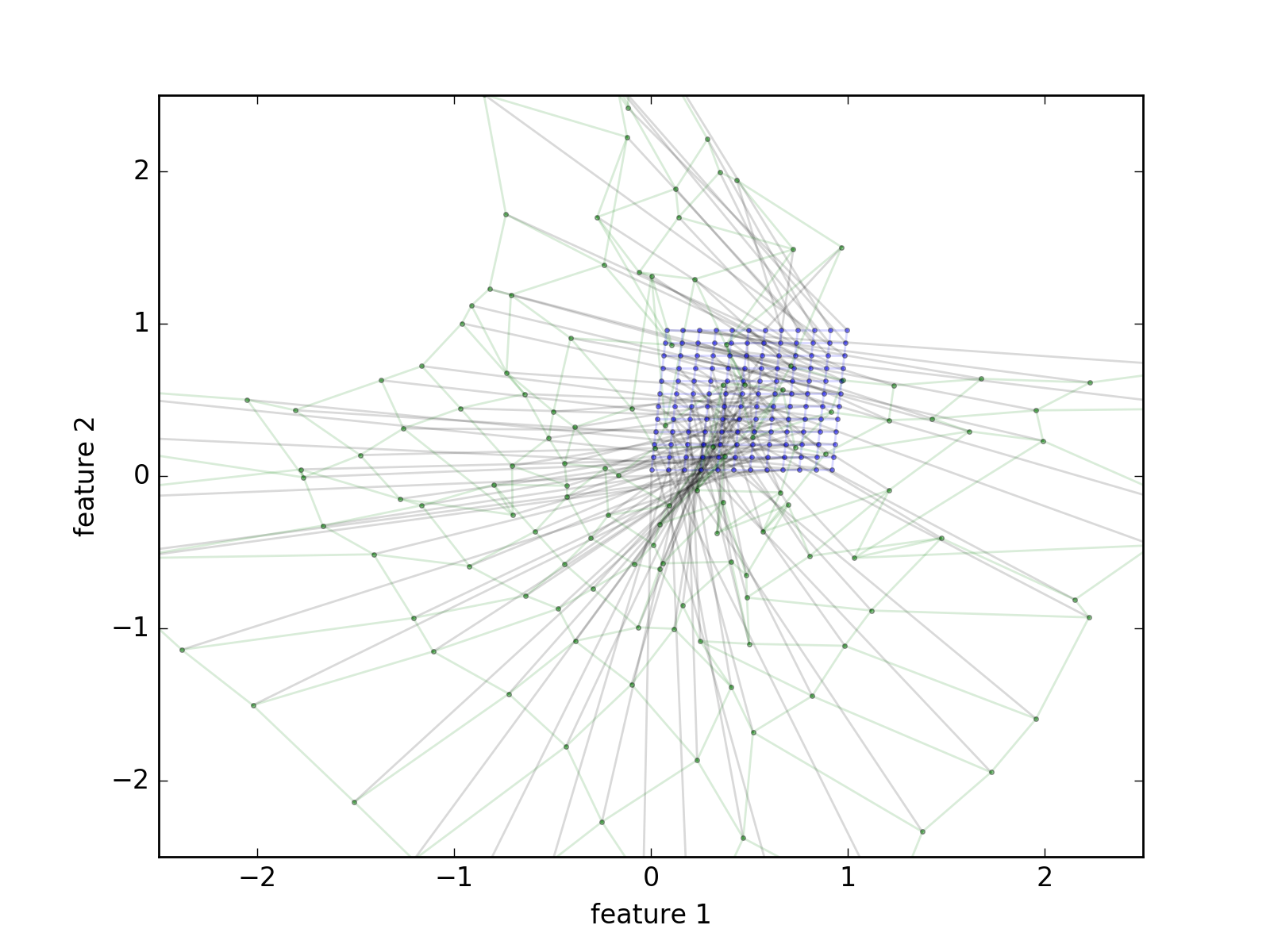
Figure 2: Ground-truth features (blue) and extracted salient features (green) for the toy experiment. Colored lines connect nodes that were neighbors in the ground truth, and black lines connect ground truth to extracted features.

3.3 WaveNet experiments

The WaveNet [23] algorithm requires conditioning to produce natural-sounding speech. Our goal was to extract 12 salient features that can be used as conditioning to produce clean speech signals from input that can be noisy or clean.

3.3.1 Databases and test procedure

We used the WSJ0 database [30] for training and testing. The training set contained 32580 utterances by 123 speakers and the test set contained 2907 utterances by 8 speakers. Additionally we used a mixed corpus of stationary and non-stationary noise from approximately 10,000 recordings captured in a variety of environments including busy streets, cafes, and pools. The inputs to the clones were 32 different versions of a signal that contains an utterance, including the clean utterance and versions with noise additions at an SNR of 0 to 10 dB. When a decoder was used, the clean signal was used as target for all decoders.

To facilitate learning, the 16 kHz signals were pre-processed into an oversampled log mel spectrogram representation. We considered two specific representations. The single window (sw) approach uses 40 ms windows with a time shift of 20 ms and 80 log mel coefficients for each time shift. In the dual window (dw) approach each 20 ms shift is associated with one window of 40 ms and two windows of 20 ms (located at 5-25, and 15-45 ms of the 40 ms window). The 20 ms windows were described with 80 log mel spectrogram coefficients, for a total of 240 coefficients for each 20 ms shift.

As reference system we used feature sets obtained with principal component analysis (PCA). It extracted 12 features (PCA12) from the 240-dimensional vector of the dual window data. The PCA was computed for the input signals of the clone-based training. Additionally, a PCA that extracts four features (PCA4) was trained as an anchor for the listening test.

We conducted a MUSHRA-like listening test on 10 utterances from the test set for 10 different speakers, using 100 human raters per utterance. The MUSHRA reference was the clean utterance. We evaluated the output of each model for both clean and noisy test utterances, except for PCA4.

3.3.2 Results

Fig. 3 shows the result of the listening test. Clone-based learning without a decoder with a single window (SalientU-sw) provides natural speech quality with good speaker identity but with fairly frequent errors for phonemes of short duration. As expected, the number of errors is lower for the clean (SalientU-sw-clean) than for noisy input signals. Learning with a decoder with a single window (SalientS-sw) reduces the errors to being very infrequent with a further small improvement for the clean input signals (SalientS-sw-clean). For the noisy input the errors are further reduced by using the dual window approach (SalientS-dw-noisy), reaching almost the quality obtained with clean input (SalientS-dw-clean and SalientS-sw-clean).

In summary, the clone-based systems with decoder significantly outperformed the reference system. This is particularly true under noisy conditions (SalientS-dw vs PCA12).

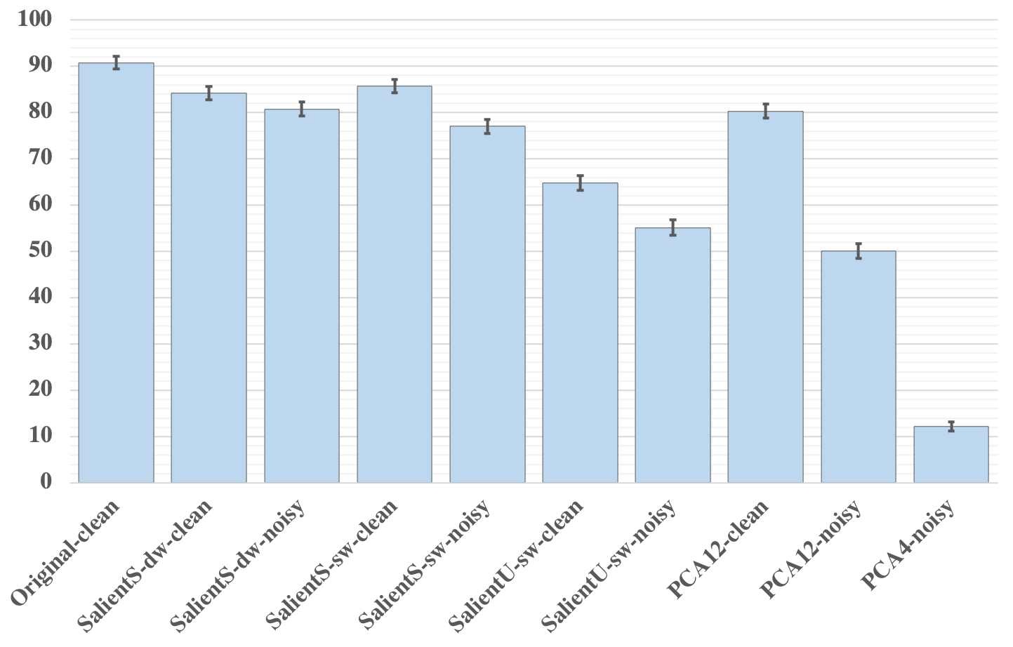
Figure 3: Listening test results.

4 Conclusion

We showed that clone-based training allows saliency to be defined in a qualitative manner by a system designer. From experiments with a toy example, we conclude that clone-based training can be used to disentangle formants from a signal. In a real-world application, the addition of a decoder improved the performance of the clone-based feature-extraction system further. The clone-based system is inherently robust to distortion and it significantly outperformed a reference system. Its natural application is coding and enhancement.

References

- [1] X. Chen, Y. Duan, R. Houthooft, J. Schulman, I. Sutskever, and P. Abbeel, “Infogan: Interpretable representation learning by information maximizing generative adversarial nets,” in Advances in Neural Information Processing Systems, 2016, pp. 2172–2180.
- [2] D. P. Kingma and M. Welling, “Auto-encoding variational Bayes,” arXiv preprint arXiv:1312.6114, 2013.
- [3] D. J. Rezende, S. Mohamed, and D. Wierstra, “Stochastic backpropagation and approximate inference in deep generative models,” arXiv preprint arXiv:1401.4082, 2014.
- [4] X. Chen, D. P. Kingma, T. Salimans, Y. Duan, P. Dhariwal, J. Schulman, I. Sutskever, and P. Abbeel, “Variational lossy autoencoder,” arXiv preprint arXiv:1611.02731, 2016.
- [5] S. Zhao, J. Song, and S. Ermon, “InfoVAE: Information maximizing variational autoencoders,” arXiv preprint arXiv:1706.02262, 2017.
- [6] A. A. Alemi, B. Poole, I. Fischer, J. V. Dillon, R. A. Saurous, and K. Murphy, “An information-theoretic analysis of deep latent-variable models,” arXiv preprint arXiv:1711.00464, 2017.
- [7] M. Phuong, M. Welling, N. Kushman, R. Tomioka, and S. Nowozin, “The mutual autoencoder: Controlling information in latent code representations,” 2017, https://openreview.net/forum?id=HkbmWqxCZ.
- [8] F. Huszar, “Is maximum likelihood useful for representation learning?” 2017, ttp://www.inference.vc/maximum-likelihood-for-representation-learning-2/.
- [9] D. Braithwaite and W. B. Kleijn, “Bounded information rate variational autoencoders,” arXiv preprint arXiv:1807.07306, 2018.
- [10] Y. Bengio, A. Courville, and P. Vincent, “Representation learning: A review and new perspectives,” IEEE transactions on pattern analysis and machine intelligence, vol. 35, no. 8, pp. 1798–1828, 2013.
- [11] C. Louizos, K. Swersky, Y. Li, M. Welling, and R. Zemel, “The variational fair autoencoder,” arXiv preprint arXiv:1511.00830, 2015.
- [12] I. Higgins, L. Matthey, A. Pal, C. Burgess, X. Glorot, M. Botvinick, S. Mohamed, and A. Lerchner, “-VAE: Learning basic visual concepts with a constrained variational framework,” in International Conference on Learning Representations, 2017.
- [13] C. P. Burgess, I. Higgins, A. Pal, L. Matthey, N. Watters, G. Desjardins, and A. Lerchner, “Understanding disentangling in -VAE,” arXiv preprint arXiv:1804.03599, 2018.
- [14] B. Esmaeili, H. Wu, S. Jain, A. Bozkurt, N. Siddharth, B. Paige, D. H. Brooks, J. Dy, and J.-W. van de Meent, “Structured disentangled representations,” stat, vol. 1050, p. 29, 2018.
- [15] H. Kim and A. Mnih, “Disentangling by factorising,” arXiv preprint arXiv:1802.05983, 2018.
- [16] N. Tishby, F. C. Pereira, and W. Bialek, “The information bottleneck method,” arXiv preprint physics/0004057, 2000.
- [17] A. A. Alemi, I. Fischer, J. V. Dillon, and K. Murphy, “Deep variational information bottleneck,” arXiv preprint arXiv:1612.00410, 2016.
- [18] W. B. Kleijn, F. S. Lim, A. Luebs, J. Skoglund, F. Stimberg, Q. Wang, and T. C. Walters, “WaveNet based low rate speech coding,” arXiv preprint arXiv:1712.01120, 2017.
- [19] R. M. Hecht and N. Tishby, “Extraction of relevant speech features using the information bottleneck method,” in Ninth European Conference on Speech Communication and Technology, 2005.
- [20] J. Bromley, I. Guyon, Y. LeCun, E. Säckinger, and R. Shah, “Signature verification using a ”Siamese” time delay neural network,” in Advances in Neural Information Processing Systems, 1994, pp. 737–744.
- [21] E. Hoffer and N. Ailon, “Deep metric learning using triplet network,” in International Workshop on Similarity-Based Pattern Recognition. Springer, 2015, pp. 84–92.
- [22] H. Kamper, W. Wang, and K. Livescu, “Deep convolutional acoustic word embeddings using word-pair side information,” in Acoustics, Speech and Signal Processing (ICASSP), 2016 IEEE International Conference on. IEEE, 2016, pp. 4950–4954.
- [23] A. van den Oord, S. Dieleman, H. Zen, K. Simonyan, O. Vinyals, A. Graves, N. Kalchbrenner, A. Senior, and K. Kavukcuoglu, “WaveNet: A Generative Model for Raw Audio,” ArXiv e-prints, Sep. 2016.
- [24] A. Gretton, K. M. Borgwardt, M. Rasch, B. Schölkopf, and A. J. Smola, “A kernel method for the two-sample-problem,” in Advances in neural information processing systems, 2007, pp. 513–520.
- [25] A. Gretton, K. M. Borgwardt, M. J. Rasch, B. Schölkopf, and A. Smola, “A kernel two-sample test,” Journal of Machine Learning Research, vol. 13, no. Mar, pp. 723–773, 2012.
- [26] M. Arjovsky, S. Chintala, and L. Bottou, “Wasserstein generative adversarial networks,” in International Conference on Machine Learning, 2017, pp. 214–223.
- [27] C. Frogner, C. Zhang, H. Mobahi, M. Araya, and T. A. Poggio, “Learning with a Wasserstein loss,” in Advances in Neural Information Processing Systems, 2015, pp. 2053–2061.
- [28] S. Hochreiter and J. Schmidhuber, “Long short-term memory,” Neural computation, vol. 9, no. 8, pp. 1735–1780, 1997.
- [29] D. P. Kingma and J. Ba, “Adam: A method for stochastic optimization,” arXiv preprint arXiv:1412.6980, 2014.
- [30] D. B. Paul and J. M. Baker, “The design for the wall street journal-based csr corpus,” in Proceedings of the workshop on Speech and Natural Language. Association for Computational Linguistics, 1992, pp. 357–362.