Astrophysics-independent determination of dark matter parameters from two direct detection signals

Abstract

Next-generation dark matter direct detection experiments will explore several orders of magnitude in the dark matter–nucleus scattering cross section below current upper limits. In case a signal is discovered the immediate task will be to determine the dark matter mass and to study the underlying interactions. We develop a framework to determine the dark matter mass from signals in two experiments with different targets, independent of astrophysics. Our method relies on a distribution-free, nonparametric two-sample hypothesis test in velocity space, which neither requires binning of the data, nor any fitting of parametrisations of the velocity distribution. We apply our method to realistic configurations of xenon and argon detectors such as XENONnT/DARWIN and DarkSide, and estimate the precision with which the DM mass can be determined. Once the dark matter mass is identified, the ratio of coupling strengths to neutrons and protons can be constrained by using the same data. The test can be applied for event samples of order 20 events, but promising sensitivities require $\gtrsim 100$ events.

I Introduction

So far dark matter (DM) has revealed its existence solely via gravitational interactions. We know its total energy density, both globally and locally, but neither its mass nor possible non-gravitational interactions are known. Motivated by the hypothesis that DM could be a WIMP (weakly interacting massive particle) Goodman and Witten (1985), there is a huge experimental effort in ton-scale noble gas direct detection (DD) experiments to search for the latter Baudis (2014); Marrodan Undagoitia and Rauch (2016); Liu et al. (2017). Several projects will test in coming years large portions of well motivated WIMP parameter space before reaching the ultimate background induced by coherent neutrino scattering.

In order to extract the DM parameters from a positive DD signal, assumptions about the local DM density and velocity distribution have to be adopted. Typically a fit is performed assuming a Maxwellian DM velocity distribution, denoted conventionally as the Standard Halo Model (SHM). It is well known that in order to pin down the DM mass, combining event spectra from experiments using different target nuclei is beneficial, exploiting the different scattering kinematics, see e.g. Refs Pato et al. (2011); Peter et al. (2014); Gluscevic et al. (2015). However, both the local energy density and the velocity distribution are subject to large uncertainties, that translate directly into uncertainties regarding the compatibility among different signals (and with upper limits) and into the DM parameters.

In this paper we show how the DM mass can be determined halo-independently from signals in two DD experiments by using a nonparametric two-sample hypothesis test. The crucial observation is that a value for the DM mass has to be adopted when transforming from recoil energy to velocity. Therefore, the normalized weighted event distributions in velocity space, which should be equal for both experiments, will only be so for the true DM mass. This method can also be applied to the case when DM–nucleus interactions are mediated by a force carrier with mass $m_{\phi}$ in the 10–100 MeV range, where both $m_{\chi}$ and $m_{\phi}$ have to be determined by the data. Furthermore, we show how the relative coupling strength of DM to protons and neutrons can be determined halo-independently from the relative number of events in two DD experiments (properly weighted in velocity space).

The method presented here builds on and extends earlier work on halo-independent methods, first proposed in Refs. Fox et al. (2011a, b) and extensively used and extended to compare different experimental results, see e.g. Refs. McCabe (2011, 2010); Frandsen et al. (2012); Herrero-Garcia et al. (2012a, b); Gondolo and Gelmini (2012); Del Nobile et al. (2013a, b); Bozorgnia et al. (2013); Frandsen et al. (2013); Feldstein and Kahlhoefer (2014a); Fox et al. (2014); Feldstein and Kahlhoefer (2014b); Cherry et al. (2014); Bozorgnia and Schwetz (2014); Gelmini et al. (2016, 2017); Ibarra and Rappelt (2017); Kahlhoefer et al. (2018); Catena et al. (2018). The basic idea of these methods is that an integral of the velocity distribution, which can be extracted from the data, should be detector-independent. They have also been extended to compare with signals of neutrinos from the Sun Blennow et al. (2015a); Ferrer et al. (2015); Ibarra et al. (2018) and with collider signals Blennow et al. (2015b); Herrero-Garcia (2015).

Various versions of halo-independent methods to determine the DM mass have been discussed previously Drees and Shan (2008); Feldstein and Kahlhoefer (2014b, a); Kavanagh and Green (2012, 2013); Kavanagh (2014), based either on fitting moments of the velocity distribution or on fitting DM mass and velocity distribution simultaneously. Our method is based on a distribution-free statistical test, which does not require any binning of data. It works for relatively small sample sizes, starting at $\gtrsim 20$ events, while more robust results can be obtained for $\gtrsim 100$ events. This is important in view of present bounds on the scattering cross section Akerib et al. (2017); Cui et al. (2017); Aprile et al. (2018) which limits the possible number of DM scattering events above the neutrino background. The method is robust with respect to energy reconstruction uncertainty and asymmetric event numbers in the two experiments.

The paper is structured as follows. In Sec. II we introduce the relevant notation for DD event rates. We describe the halo-independent method to extract the DM mass in Sec. III, while in Sec. IV we explain how to extract the ratio of couplings to protons and neutrons. In Sec. V we show how the test can be applied in case of an interaction mediated by a light mediator. We give our conclusions in Sec. VI.

II The direct detection event rate

For DM scattering elastically off single-target detectors with spin-independent (SI) interactions, the time-averaged differential event rate is given by

$$\dfrac{dR_{D}}{dE_{R}}=\frac{\rho_{\chi}\bar{\sigma}A_{{\rm eff},D}^{2}}{2m_{\chi}\mu_{p}^{2}}F^{2}_{D}(E_{R})\underbrace{\int_{v>v_{\text{m},D}}d^{3}v\,\frac{f\left(\vec{v}+\vec{v}_{e}\right)}{v}}_{\equiv\eta(v_{\text{m},D})}\,,$$ (1)

where by kinematics

$$v_{\text{m},D}=\sqrt{\frac{m_{A_{D}}E_{R}}{2\,\mu_{A_{D}}^{2}}}$$ (2)

is the minimum DM velocity that detector $D$ is sensitive to for a given recoil energy $E_{R}$. Following the notation of Ref. Schwetz and Zupan (2011), we define an effective target mass number by

$$A_{{\rm eff},D}^{2}\equiv 2[Z_{D}\cos\theta+(A_{D}-Z_{D})\sin\theta]^{2}\,,$$ (3)

with $\tan\theta\equiv f_{n}/f_{p}$ being the ratio of couplings to neutrons $f_{n}$ and protons $f_{p}$, and $\bar{\sigma}=(\sigma_{p}+\sigma_{n})/2$ the zero-momentum transfer cross section for DM–nucleon scattering averaged over scattering on protons and neutrons. If several isotopes of an element are present in the detector, Eq. (3) has to be replaced by a sum over the isotopes, weighted by the relative abundance Schwetz and Zupan (2011). Furthermore, $m_{A_{D}}$ is the mass of the target nucleus in experiment $D$, $\mu_{p}\,(\mu_{A_{D}})$ is the proton (nucleus) reduced mass, and $F_{D}(E_{R})$ is the SI nuclear form factor. $f(\vec{v})$ describes the distribution of DM particle velocities in the galaxy rest frame, and $\rho_{\chi}$ is the DM local energy density. For our simulations, we adopt the Helm parametrisation for $F_{D}(E_{R})$, and we use the SHM, i.e., a Maxwellian velocity distribution, cut-off at the galactic escape velocity $v_{\rm esc}=544\,{\rm km/s}$, and with local energy density $\rho_{\chi}=0.4\,{\rm GeV\,cm^{-3}}$ McCabe (2010). We neglect the time-dependent velocity of the Earth around the Sun.

The total number of events in detector $D$ above the energy threshold $E_{{\rm th},D}$ is given by

$$n_{D}=M_{D}T_{D}\int_{E_{{\rm th},D}}dE_{R}\,\dfrac{dR_{D}}{dE_{R}}\,,$$ (4)

where $M_{D}T_{D}$ is the exposure (detector mass times measurement time). We ignore here possible detector- and energy-dependent resolution and efficiency functions. We comment later on their impact.

Xe/Ar	$M_{D}T_{D}$ [t yr]	$E_{\rm th}$ [keV]	# of events
$m_{\chi}$ [GeV]			20	50	100
Conservative	10/20	5/10	52/23	117/45	89/38
Optimistic	40/40	3/8	357/59	569/99	410/83

Table 1: Parameters of our default configurations for the xenon/argon DM experiments denoted as conservative and optimistic. We give the assumed exposure (detector mass $M_{D}$ times measurement time $T_{D}$) and the energy thresholds. The last three columns show the expected number of events for DM masses of 20, 50, and 100 GeV, assuming a fiducial SI cross section of $\bar{\sigma}=5\times 10^{-47}$ cm² generated by a heavy mediator, and equal couplings to neutrons and protons.

For our numerical calculations we simulate realistic realizations of xenon and argon experiments, as several experiments using these targets are planned: LZ Akerib et al. (2015), PandaX Cui et al. (2017), XENONnT Aprile et al. (2014), and ultimately DARWIN Aalbers et al. (2016), using xenon; DEAP-3600 Fatemighomi (2016), ArDM Calvo et al. (2017), DarkSide and Argo Aalseth et al. (2018), using argon. In Tab. 1 we define two benchmark configurations which we denote as conservative and optimistic. For comparison, XENONnT and LZ plan for detector masses of order 10 t, while the goal of DARWIN is 40 t of xenon. The DarkSide collaboration envisages a 20 t (100 t) argon detector mass for DarkSide-20k (Argo). The event numbers quoted in the table are obtained for a fiducial cross section of $\bar{\sigma}=5\times 10^{-47}$ cm², close to the current XENON1T limit Aprile et al. (2018). For a zero-background experiment event numbers are proportional to the product $M_{D}T_{D}\bar{\sigma}$. The assumed energy thresholds are motivated by those achieved by the currently running experiments, as well as the target numbers quoted in the respective proposals, taking into account the zero-background assumption. In our numerical analysis, we generate many instances (typically $10^{3}$) of recoil energy event distributions for the two experiments by Monte Carlo, with the total number of events drawn from a Poisson distribution with mean given by Eq. (4).

III Extracting the dark matter mass

The key observation used in halo-independent methods is that, while the prefactor in Eq. (1) depends on the target nucleus, $\eta(v_{\rm m})$ is a detector-independent quantity Fox et al. (2011a, b). Therefore, if two signals are observed in detectors using different targets, one can compare their properly weighted distributions in the overlapping velocity space for different DM masses, and they will only agree for the true DM mass. In the following we will employ a non-parametrical two-sample hypothesis test to infer the correct DM mass from two DD event samples.

Suppose detectors 1 and 2 observe $n_{1}$ and $n_{2}$ DM induced events, respectively, with certain recoil energies $E_{R}^{i,D}$, where $i=1,...,n_{D}$, $D=1,2$. For an assumed value of the DM mass $m_{\chi}$, these recoil energies can be transformed into velocities via Eq. (2). It is more convenient to work with the square of the minimal velocity, since then the Jacobian of the transformation is just a constant. Therefore we define the transformed event samples $x_{i}=v_{i,1}^{2}(m_{\chi})$ and $y_{j}=v_{j,2}^{2}(m_{\chi})$. If the true value for $m_{\chi}$ has been used in this transformation, the random variables $x_{i}$ and $y_{j}$ will be distributed according to probability distribution functions (PDF) proportional to $F^{2}_{1}(v^{2})\eta(v^{2})$ and $F^{2}_{2}(v^{2})\eta(v^{2})$, respectively. We can now weigh the distribution of each experiment with the form factor of the other experiment. We define

$$h(v^{2}) \equiv F^{2}_{1}(v^{2})F^{2}_{2}(v^{2})\eta(v^{2})\,,\quad$$ (5)

$$\tilde{h}(v^{2}) \equiv{\mathcal{N}}\,h(v^{2})\quad\text{with}\quad\int_{v^{2}_{\rm m,th}}dv^{2}\tilde{h}(v^{2})=1\,,$$ (6)

where ${\mathcal{N}}$ is a normalization constant and in the arguments of the form factors $F_{D}^{2}(v^{2})$ velocity is converted into energy using the relation corresponding to the experiment $D$, see Eq. (2). By construction the PDF $\tilde{h}(v^{2})$ will be identical for the two event samples, if the correct DM mass is used to convert recoil energy into squared-velocities.

In order to apply this idea to the data samples $x_{i}$ and $y_{j}$ we consider the corresponding cumulative distribution function (CDF), $H(v^{2})=\int_{v^{2}_{\rm m,th}}^{v^{2}}dx\,\tilde{h}(x)$. It can be estimated from the two data samples in the following way:

$$\hat{H}_{(1)}(x) =\frac{1}{\omega_{\rm t,1}}\sum_{i=1}^{n_{1}}1_{x_{i}\leq x}\,\omega_{i,1}\,,$$

$$\hat{H}_{(2)}(x) =\frac{1}{\omega_{\rm t,2}}\sum_{j=1}^{n_{2}}1_{y_{j}\leq x}\,\omega_{j,2}\,,$$ (7)

where $1_{x_{i}\leq x}$ is equal to 1 for $x_{i}\leq x$, and zero otherwise, and

$$\omega_{i,1}\equiv F^{2}_{2}[E_{R,2}(v^{2}_{i,1})]\,,\quad\omega_{\rm t,1}\equiv\sum_{i=1}^{n_{1}}\omega_{i,1}$$ (8)

and similar for the weights $\omega_{j,2}$ of the events $y_{j}$ of the second sample. As we normalize by the sum of the weights, the prefactors and the Jacobian of the transformation to velocity space drop out. The lower integration boundary $v^{2}_{\rm m,th}$ in Eq. (6) is determined by the energy thresholds of the two detectors: for a given DM mass $m_{\chi}$ the two recoil energy thresholds are transformed into velocity-squared using Eq. (2) and $v^{2}_{\rm m,th}$ is chosen as the larger of the two. The sums in Eqs. (7) and (8) include only events with $x_{i},y_{j}>v^{2}_{\rm m,th}$. This ensures that only events which probe overlapping regions in $v^{2}$-space are considered. Note that in certain cases there will be no events in the overlapping region. In these cases our test cannot be applied.

Several standard statistical tools are available to test whether two empirical CDFs emerge from the same underlying PDF (which is the null hypothesis in the following), for instance the Kolmogorov-Smirnov, Cramér-von Mises, or Anderson-Darling tests, see e.g., Ref. Monahan (2011). In the following we will present results based on the Cramér-von Mises (CvM) test, which for our application shows somewhat better statistical properties than alternative tests. The corresponding test statistic $T_{\rm CvM}$ is defined as

$$\frac{(\tilde{n}_{1}+\tilde{n}_{2})^{2}}{\tilde{n}_{1}\tilde{n}_{2}}T_{\rm CvM} =\sum_{i=1}^{n_{1}}\left[\hat{H}_{(1)}(x_{i})-\hat{H}_{(2)}(x_{i})\right]^{2}$$

$$+\sum_{j=1}^{n_{2}}\left[\hat{H}_{(1)}(y_{j})-\hat{H}_{(2)}(y_{j})\right]^{2}\,,$$ (9)

and it has a known asymptotic distribution under the null hypothesis Anderson and Darling (1952), which can be used to calculate a $p$-value for a given observed value $T_{\rm CvM}^{\rm obs}$, i.e., the probability of obtaining $T_{\rm CvM}>T_{\rm CvM}^{\rm obs}$. The effective event numbers $\tilde{n}_{D}\equiv(\sum\omega_{i,D})^{2}/\sum\omega_{i,D}^{2}$ in Eq. (9) take into account that the actual events have been drawn from the unweighted distribution Monahan (2011). The null hypothesis (i.e., the samples emerge from the same PDF) corresponds to the case that the correct DM mass has been used to convert from recoil energy to velocity-squared space. Hence, in the plots below we will show the $p$-value as proxy of the discriminating power for the DM mass: a low $p$-value will indicate that the null-hypothesis has to be rejected at a certain confidence level, and therefore that particular value of the DM mass as well. We have checked, by explicit Monte Carlo simulations of DM events, that under the null-hypothesis the test statistic defined as in Eq. (9) indeed follows the known distribution for the CvM statistic, despite the re-weighting of the data necessary to cope with the form factors.

The method can also serve to test if two signals are compatible with each other under the DM hypothesis: if the $p$-value is small for any DM mass, then one can conclude that at least one of the signals is not consistent with the underlying DM hypothesis (e.g. elastic scattering, spin-independent interactions). This is independent of whether the couplings are isospin-conserving or violating (see also below).

III.1 Numerical results

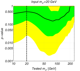
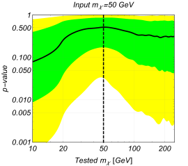
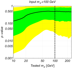
Figure 1: $p$-value for the tested dark matter mass, for different values of input DM mass shown as dashed vertical lines: $20$ GeV (left), $50$ GeV (middle) and $100$ GeV (right). The conservative configuration has been assumed (see Tab. 1). We have generated $10^{3}$ random data samples. The black curve corresponds to the median $p$-value, whereas the shaded green and yellow regions indicate the range of $p$-values obtained in 68% and 95% of the cases, respectively.

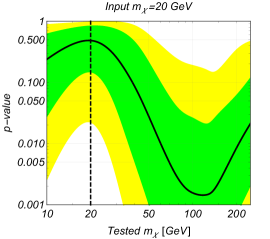
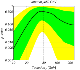
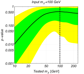
Figure 2: Same as Fig. 1 but assuming the optimistic configuration (see Tab. 1).

In Figs. 1 and 2 we show the results of the numerical analysis for the conservative and optimistic experimental configurations defined in Tab. 1, respectively. We have generated $10^{3}$ random realizations of the experiments, by assuming fixed true DM masses of 20, 50, and 100 GeV. For a given true DM mass we then calculate the $p$-value of each random data sample as a function of $m_{\chi}$ (denoted “tested” DM mass). The plots show the median of the $p$-values (black curves), as well as the range of $p$-values obtained in 68% and 95% of the cases (green and yellow bands).

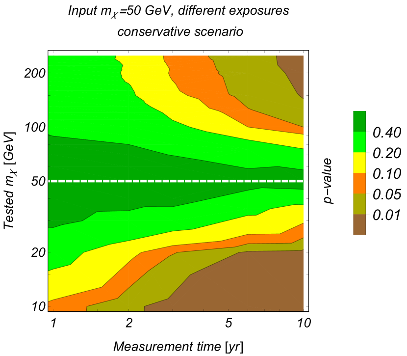
Figure 3: Median $p$-value of the reconstructed (tested) DM mass as a function of measurement time, for an assumed true DM mass of 50 GeV. We adopt the conservative configuration from Tab. 1 with detector masses of 10/20 t for xenon/argon.

First, we observe that there is a rather large spread in the $p$-values. E.g., while the median $p$-values for the conservative configuration are generally above 0.1, there is a rather high chance that much stronger discrimination can be obtained, with $p$-values even below 0.01, c.f. Fig. 1. Conversely, even for the optimistic configuration chances are high that discrimination against wrong DM masses is poor, c.f. Fig. 2. Second, focusing on the median $p$-value, we see that for significant DM mass determinations exposures similar to the optimistic case may be required, i.e., a few hundreds of events in xenon and around 100 events in argon. From Fig. 2 we see that for the average optimistic configuration, DM masses of 20 and 50 GeV, can be determined at the 90% CL to be in the ranges [7, 38] and [21, 190] GeV, respectively, and $m_{\chi}=100$ GeV can be constrained to be $\geq 23$ GeV. In Fig. 3 we show the uncertainty with which a true DM mass of 50 GeV can be determined as a function of the measurement time. We observe roughly a scaling with the square-root of the exposure. After a 10 year exposure for our benchmark cross section and detector masses the range can be constrained at 90% CL to [30, 90] GeV.

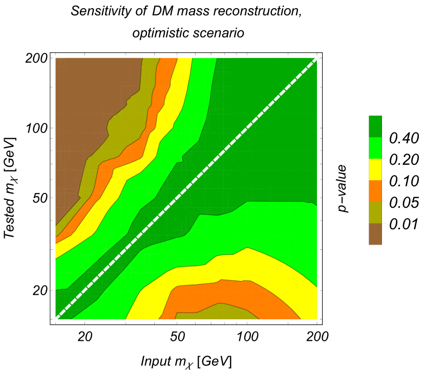
Figure 4: Contours of median $p$-value of the reconstructed (tested) DM mass as a function of the true (input) DM mass for the optimistic configuration defined in Tab. 1.

The precision with which $m_{\chi}$ can be determined as a function of the true DM mass is shown in Fig. 4 for the median optimistic configuration. We see that the test works fine for DM masses in the range approximately from 20 to 70 GeV. For larger DM masses only a lower bound can be obtained. This is to be expected, since for $m_{\chi}\gg m_{A}$, $v_{\rm m}$ and therefore $\eta(v_{\rm m})$ become independent of the DM mass, c.f. Eq. (2). This behaviour is not specific to our test; it follows from general kinematics and any DM determination from DM–nucleus scattering has this property. Note that for calculating Fig. 4 we fix $M_{D}T_{D}\bar{\sigma}$ to the value defined in Tab. 1. This implies that the event rate decreases linearly with $m_{\chi}$ for $m_{\chi}\gg m_{A}$, see Eqs. (1) and (4). This explains the decrease of the lower bound on $m_{\chi}$ for input values $\gtrsim 100$ GeV in Fig. 4. We have checked that if event numbers are kept constant when changing the true $m_{\chi}$ the lower bound remains approximately constant.

Let us comment on the increase of the $p$-value visible for large DM masses in the case of true $m_{\chi}=20$ GeV (left panels in Figs. 1 and 2). In this region it may happen, that the events of the two experiments fall into distinct regions in $v_{\rm m}$ space, i.e., there is no overlapping range of $v_{\rm m}$ values. The exact region in which this occurs is, to some extent, a consequence of the SHM assumption and the escape velocity used in generating our events. In such cases the test cannot be applied and formally the test statistic is zero, indicating that data is consistent with the null-hypothesis, i.e., such values of the DM mass can be consistent with the data. In such a case other diagnostic tools have to be employed, to find out whether data are consistent. For instance, one could check whether the situation of non-overlapping events in $v_{\rm m}$-space is consistent with the fact that $\eta(v_{\rm m})$ has to be a decreasing function (which would require an additional assumption on the ratio of couplings to neutrons and protons, though).

III.2 Robustness against energy resolution and background

In the previous analysis, we have assumed perfect energy resolution and efficiency and zero background. In order to study whether our method is robust also in less ideal situations we have introduced a constant gaussian energy resolution when generating the Monte Carlo data, but still assume perfect resolution when applying the DM mass test. We find that for energy resolutions below $2$ keV the test results are essentially unmodified. Similarly, we also simulated the case of constant or exponential backgrounds in the data, but ignoring it when applying the test. The discriminating power of our method is found to be unaffected as long as the background is below roughly $10\%$ of the DM signal. Both results illustrate that indeed the method can be realistically applied when two signals are observed.

We have also checked that the test performs slightly better for similar number of events in both experiments (therefore it is desirable to have a larger exposure for argon than for xenon, for example). Note however, that our benchmark scenarios defined in Tab. 1 have rather asymmetric event numbers, and therefore our test works also fine if one of the two experiments has less events than the other.

IV Ratio of couplings to neutrons and protons

Let us assume that the DM mass can be determined with sufficient precision. Then it is possible to use the data from the two experiments to constrain also the ratio of couplings to neutrons and protons, i.e., $\theta=\arctan{(f_{n}/f_{p})}$, see Eq. (3). For simplicity we focus on the heavy mediator case, for the generalization to light mediators see section V, and in particular footnote 4. Let us consider the following quantities:

$$q_{D}\equiv M_{D}T_{D}\frac{\rho_{\chi}\bar{\sigma}}{m_{\chi}\,m_{A_{D}}}\frac{\mu_{A_{D}}^{2}}{\mu_{p}^{2}}A_{{\rm eff},D}^{2}\int_{v^{2}_{{\rm m,th}}}dv^{2}h(v^{2})\,,$$ (10)

with $h(v^{2})$ defined in Eq. (5), $v^{2}_{{\rm m,th}}$ determined as described above, and where we have taken into account the Jacobian from changing integration variables from $E_{R}$ to $v^{2}$. We see that the ratio

$$\frac{q_{1}m_{A_{1}}/(M_{1}T_{1}\mu_{A_{1}}^{2})}{q_{2}m_{A_{2}}/(M_{2}T_{2}\mu_{A_{2}}^{2})}=\frac{A_{\rm eff,1}^{2}(\theta)}{A_{\rm eff,2}^{2}(\theta)}$$ (11)

only depends on $\theta$ and is independent of the halo integral as well as global factors such as the total cross section and the local DM density. The quantity $q_{D}$ can be estimated from data. Indeed, it corresponds to the total weights defined in Eq. (8), which are obtained by evaluating the form factor of the other experiment at the recoil energies of the observed events:

$$\hat{q}_{D}=\omega_{\rm t,D}\,.$$ (12)

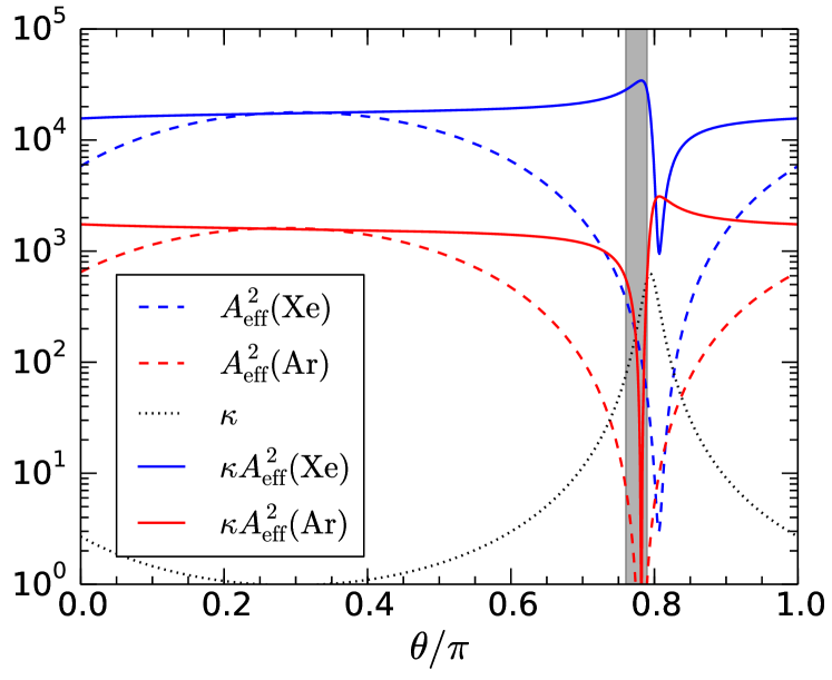
Figure 5: Effective mass numbers-squared (dashed) and rescaled ones (solid) for xenon (blue) and argon (red), and the applied rescale factor (dotted) are shown as a function of $\theta={\rm arctan}(f_{n}/f_{p})$, with $f_{n}$ and $f_{p}$ being the coupling to neutron and proton, respectively. The shaded region indicates the range where the event rate in argon detectors is strongly suppressed.

In Fig. 5 we show the effective mass number squared for xenon and argon (dashed curves). Event numbers are strongly suppressed if $\tan\theta\approx-Z/(A-Z)$. We see from the plot that this cancellation happens for $\theta\approx 0.8\pi$ for both elements. Argon detectors employ depleted argon which consists basically only of ⁴⁰Ar. Therefore the cancellation can be complete. For xenon we take into account the natural isotope composition, and therefore the cancellation is never exact. In order to maintain events for at least one detector, we rescale the effective cross section by an arbitrary factor $\kappa(\theta)$, shown as dotted curve in the plot. It has been chosen in such a way that the number of events remain approximately constant also close to the cancellation region, at least for one of the two experiments, see solid curves in Fig. 5. Obviously, if one of the experiments does not see events, the DM mass cannot be determined, and therefore our method cannot be applied. This case is indicated by the shaded region, where the event rate in the argon experiment is strongly suppressed. Note that due to the isotope distribution in xenon, we can have sizeable event numbers for xenon even close to the cancellation region.

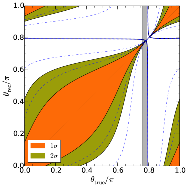
Figure 6: Reconstructed relative coupling to neutrons and protons as a function of the true value for the optimistic experimental configuration with re-scaled event numbers as shown in Fig. 5. For a given $\theta_{\rm true}$, the interval in $\theta_{\rm rec}$ corresponding to the white region can be excluded at $2\sigma$. Dashed curves indicate the $1\sigma$ and $2\sigma$ regions for the conservative configuration. The analysis assumes that the DM mass is known. In the grey-shaded region the event rate in argon is strongly suppressed and therefore the DM mass cannot be determined with our method in that region.

For the numerical analysis we have extracted the empirical values $\hat{q}_{D}$ for a large number of random realizations of our benchmark xenon and argon experiments, assuming a DM mass of 50 GeV, and calculated the variance of $q_{D}$ from the samples. Then the precision with which $\theta$ can be determined from the data can be estimated with a simple $\chi^{2}$ analysis, fitting the predicted values $q_{1}$ and $q_{2}$ as a function of $\theta$ to the empirical ones. The result is shown in Fig. 6. We see that for true values far from the cancellation region around $0.8\pi$, we can exclude that $\theta$ is close to $0.8\pi$. If the true value is around the cancellation region and sufficient events are obtained in both detectors that the mass can be reconstructed, then $\theta$ can be determined very accurately with our method. This behaviour is obvious from Eq. (11) and Fig. 5.

Note, however, that there is always a degeneracy in the determination of $\theta$, visible in the plot by the nearly horizontal/vertical strips. The origin of the degeneracy is related to the sign-ambiguity in Eq. (11), since only the ratio of the squares of the $A_{\rm eff}$ in both experiments can be determined. Therefore, when solving for $\theta$, there are always two possible sign combinations, with only one of them corresponding to the true $\theta$. In the single-isotope approximation the degeneracy is located at

$$\tan\theta_{\rm deg}=-\frac{2Z_{1}Z_{2}+(Z_{1}N_{2}+Z_{2}N_{1})\tan\theta_{\rm true}}{Z_{1}N_{2}+Z_{2}N_{1}+2N_{1}N_{2}\tan\theta_{\rm true}}\,,$$ (13)

with $N_{D}=A_{D}-Z_{D}$, in excellent agreement with the numerical result in Fig. 6. As is clear from the plot, the degeneracy remains also in the presence of multiple isotopes in xenon. The only way to resolve this degeneracy is to consider events in three different target materials, with sufficiently different proton-to-neutron ratios. The generalization of our method to three experiments is straight forward. For instance, the product of all three form factors has to be included in the distribution $h(v^{2})$ defined in Eq. (5), and so on. A detailed study of this case is beyond the scope of this work.

Let us remark that the total cross section $\bar{\sigma}$ cannot be extracted halo-independently. DM velocity distribution independent lower limits on the product $\rho_{\chi}\bar{\sigma}$ can be obtained from averaged rates Blennow et al. (2015b) and, if observed, from annual modulations Herrero-Garcia (2015). The bounds derived there can be evaluated for the DM mass extracted by applying the method developed in the present work.

V Light mediators

The method explained so far can be directly applied to any differential cross section that is factorizable as the product of velocity and energy-dependent parts. Any extra energy-dependent factor, coming from the differential cross section or from a DM form factor, can be treated in an analogous way as the nuclear form factor. As an example, we now assume that the interaction is mediated by a light mediator, with mass $m_{\phi}$, chosen to be in the 10–100 MeV range. Following the notation of Ref. Schwetz and Zupan (2011), this situation can be parametrized by an extra energy-dependent factor in the differential event rate Eq. (1):

$$G_{D}(E_{R})\equiv\frac{(2m_{A_{D}}E_{{\rm th},D}+m^{2}_{\phi})(2m_{A_{D}}E_{\rm ref}+m^{2}_{\phi})}{(2m_{A_{D}}E_{R}+m^{2}_{\phi})^{2}}\,,$$ (14)

where $E_{\rm ref}$ is an arbitrary reference recoil energy, which we have set to the value corresponding to $v_{\rm m}=200$ km/s for a given DM mass according to Eq. (2). To take the additional recoil energy dependence into account in our test, one has to make the replacement

$$F_{D}^{2}(E_{R})\to F_{D}^{2}(E_{R})G_{D}(E_{R})$$ (15)

in all expressions. Note that a light mediator actually does not modify the $v_{\rm m}$ distribution itself, but just enters our analysis in the weight factors. The numerator in Eq. (14) drops out and we see that the finite mediator mass will only enter into the CDF in Eq. (7) if $2m_{A_{D}}E_{R}\simeq m^{2}_{\phi}$. Also, for very light mediators, $2m_{A_{D}}E_{R}\gg m^{2}_{\phi}$, the mediator mass is irrelevant and the dependence on the different targets via $m_{A_{D}}$ becomes a multiplicative factor which drops out. Hence, we expect that our test, which is only sensitive to non-trivial modifications which are different for the two detectors, will only be sensitive to the case $2m_{A_{D}}E_{R}\simeq m^{2}_{\phi}$.

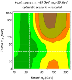
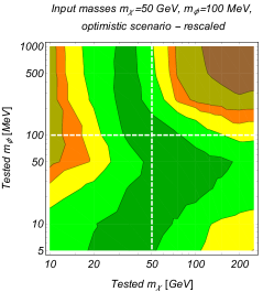
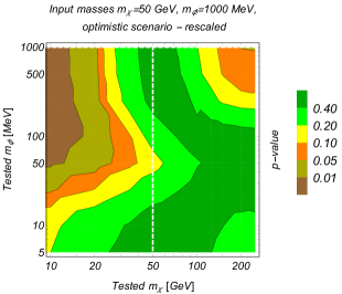
Figure 7: Contours of the median $p$-value for the light mediator model in the $m_{\phi}$ – $m_{\chi}$ plane. The input values are indicated by the dashed lines and quoted in the figure headings. We use the optimistic configuration and rescale the cross section such that we obtain mean Xe/Ar event numbers of 760/187, 770/154 and 849/149 for the left, middle and right panels, respectively.

In Fig. 7 we show contour plots of the $p$-value in the parameter space of tested masses, $m_{\phi}$ – $m_{\chi}$, for three examples of input masses. We have considered the optimistic scenario and rescaled the total cross section such that event numbers for our three example points are similar, around 800/160 for Xe/Ar. In all three cases we see that it is difficult to determine the mediator mass with our test, for the reasons discussed above, and we observe a degeneracy between $m_{\phi}$ and $m_{\chi}$. For the considered experimental configurations the condition $2m_{A_{D}}E_{R}\simeq m^{2}_{\phi}$ is fulfilled for $m_{\phi}\simeq 30$ MeV, clearly visible in the plots. A value of $m_{\phi}$ in that region can be compensated by a larger value of $m_{\chi}$, while—in agreement with the argument presented above—the test cannot distinguish between $m_{\phi}$ much larger and much smaller than 30 MeV, for similar values of $m_{\chi}$. Although event spectra for $m^{2}_{\phi}\gg$ or $\ll 2m_{A_{D}}E_{R}$ look quite different, our test is not designed to distinguish between different spectra itself, but tests differences between the weighted $v_{\rm m}$ distributions between the two experiments, which indeed may be identical for the two extreme cases. Clearly additional tests have to be applied to distinguish those cases, in particular whether data would be compatible with a physically reasonable halo model. Despite those limitations of our test, we see from Fig. 7 that in all cases certain regions in the $m_{\phi}$ – $m_{\chi}$ plane can be excluded completely halo-independently and without any assumption about the neutron-proton couplings ratio.

VI Conclusions and outlook

In the next years significant progress in DM direct detection experiments is to be expected. If finally a DM signal is seen, it is just a matter of time that a signal in a different target detector is also observed. Once this happens, one needs a way to accurately extract the DM parameters by taking into account uncertainties in astrophysical parameters, in particular the DM velocity distribution and its local energy density. In this work, we have developed a simple halo-independent method to extract the DM mass and the ratio of couplings to neutrons and protons by comparing two DD signals. It is a distribution-free, non-parametric hypothesis test in velocity space, which does not require any binning of the data. Our proposed test is sensitive to the shape of the integrated velocity distribution, which has to be identical for the different event samples when converting from nuclear recoil energies to velocity with the correct value of the DM mass.

We have applied the test to mock data from realistic xenon and argon experiments, such as the DARWIN and DarkSide projects. The test works best for values of the DM mass between the masses of the two detector nuclei, which have to be sufficiently different. For heavy DM masses, only a lower bound can be obtained (as for any method to extract the DM mass from DM–nucleus scattering data). For example, a DM mass of 50 GeV can be constrained with our test to the interval [21, 190] GeV at $90\,\%$ CL if 570/100 events are observed in Xe/Ar. If 1200/450 events are available, the interval shrinks to [30, 90] GeV. While the precision is limited, we stress that those results would be completely independent of any astrophysical assumption, and therefore more robust. Furthermore, we have presented a method to constrain the ratio of DM couplings to neutrons and protons, which can be applied to the same data, once the DM mass has been determined.

A crucial input for the analysis are nuclear form factors. Therefore, an assumption about the type of interaction is necessary. In our study we have assumed spin-independent interactions. Generalizations to other interactions (e.g., spin-dependent) are straight-forward. One explicit example we have considered is a light mediator particle, which effectively leads to a modified form factor. In that case we find that a determination of the mediator mass based on our test is difficult, however, certain regions in the DM/mediator masses parameter space can be disfavoured completely halo-independently.

Let us stress that the test uses an absolutely minimal assumption about the DM distribution, namely that the shape of the DM velocity distribution seen by the two detectors is the same. It is not guaranteed that the signals are compatible with a physically meaningful DM distribution. For instance, the requirement that $\eta(v_{\rm m})$ has to be a decreasing function is not built in the test and should be checked independently. Once the DM mass has been determined to some precision, the data can be used to reconstruct the DM distribution, for instance by methods similar to the ones discussed in the literature, e.g., Drees and Shan (2007); Kavanagh (2014); Feldstein and Kahlhoefer (2014b). This will be an important consistency check, to see whether the data are consistent with a physically reasonable DM distribution.

Finally, our test or modifications thereof can be applied to a possible annual modulation signal, to generalized DM–nucleon interactions with different momentum and/or velocity dependence, to inelastic scattering, or to multi-component DM. We leave the exploration of such cases for future work.