MiNNLO_PS: A new method to match NNLO QCD to parton showers

MINNLO${}_{\text{PS}}$: A new method to match NNLO QCD to parton showers

Abstract

We present a novel method to combine QCD calculations at next-to-next-to-leading order (NNLO) with parton shower (PS) simulations, that can be applied to the production of heavy systems in hadronic collisions, such as colour singlets or a $t\bar{t}$ pair. The NNLO corrections are included by connecting the MiNLO^′ method with transverse-momentum resummation, and they are calculated at generation time without any additional reweighting, making the algorithm considerably efficient. Moreover, the combination of different jet multiplicities does not require any unphysical merging scale, and the matching preserves the structure of the leading logarithmic corrections of the Monte Carlo simulation for parton showers ordered in transverse momentum. We present proof-of-concept applications to hadronic Higgs production and the Drell-Yan process at the LHC.

1 Introduction

Particle phenomenology at the Large Hadron Collider (LHC) has entered the precision era. After the landmark discovery of the Higgs boson Aad:2012tfa ; Chatrchyan:2012xdj , which explains the electroweak (EW) symmetry breaking and completes the particle content predicted by the Standard Model (SM), the LHC is now focussing upon the search for hints of new-physics phenomena. Despite several indications that there must be physics beyond the SM (BSM) at relatively low scales, as of now new-physics searches at the LHC have been unsuccessful. In this scenario, precision measurements have become of foremost importance, as they enhance the sensitivity of indirect searches for new physics through small deviations from SM predictions.

Modifications of the electroweak sector, induced by many BSM theories, can be unravelled through precision studies of electroweak interactions. Both the production of a Higgs-boson and of EW vector bosons play a crucial role in this respect. Notably, for the Drell-Yan process the experimental uncertainties have already surpassed the percent level Aaboud:2017ffb ; Sirunyan:2017igm ; Aaboud:2017svj . On the theory side, predictions have to be controlled at the same level of precision, which demands calculations with at least next-to-next-to-leading order (NNLO) accuracy in QCD perturbation theory. Furthermore, the experimental measurements operate at the level of hadronic events and require full-fledged Monte Carlo simulations in their analyses. The inclusion of NNLO QCD corrections in event generators is therefore mandatory to fully exploit LHC data.

In this paper, we present a novel method to perform the consistent matching of NNLO calculations and parton showers (hereafter NNLO+PS), based on the structure of transverse-momentum resummation. Our method builds upon MiNLO Hamilton:2012np , a procedure for improving NLO multijet calculations with the appropriate choice of scales and with the inclusion of Sudakov form factors, that is particularly suited to be interfaced with parton-shower generators using the POWHEG method. In ref. Hamilton:2012rf the MiNLO procedure was refined in such a way that, in processes involving the production of a massive colour singlet system in association with one jet, the NLO accuracy is formally retained also for observables inclusive in the jet. Such procedure, dubbed MiNLO^′, yields an NLO multi-jet merging method that does not use a merging scale. Notably, a numerical method to extend the MiNLO^′ procedure to more complex processes, and its application to Higgs production in association with up to two jets, was presented in ref. Frederix:2015fyz .

In this article we extend the MiNLO^′ method to achieve NNLO accuracy at the fully differential level in the zero-jet phase space, while retaining NLO accuracy for the one-jet configurations. Our method will be referred to as MiNNLO_PS in the following, and it has the following features:

• NNLO corrections are calculated directly during the generation of the events, with no need for further reweighting.

• No merging scale is required to separate different multiplicities in the generated event samples.

• When combined with transverse-momentum ordered parton showers, the matching preserves the leading logarithmic structure of the shower simulation.

Maintaining the logarithmic accuracy of the shower is a crucial requirement of all NLO+PS, and a fortiori NNLO+PS approaches. We stress that this requirement is immediately met by the MiNNLO_PS approach, that works by generating the first two hardest emissions and letting the shower generate all the remaining ones. We also recall that, if the shower ordering variable differs from the NLO+PS one, maintaining the Leading Logarithmic accuracy of the shower becomes a delicate issue. An example is given by a POWHEG based generator interfaced to an angular-ordered shower. To preserve the accuracy of the shower, not only one needs to veto shower radiation that has relative transverse momentum greater than the one generated by POWHEG, but also one has to resort to truncated showers to compensate for missing collinear-soft radiation. Failing to do so spoils the shower accuracy at leading-logarithmic level (in fact, at the double-logarithmic level).

Three different NNLO+PS approaches have been previously formulated in the literature Hamilton:2012rf ; Alioli:2013hqa ; Hoeche:2014aia and applied to the simplest LHC processes, namely Higgs-boson production Hamilton:2013fea ; Hoche:2014dla and the Drell-Yan process Hoeche:2014aia ; Karlberg:2014qua ; Alioli:2015toa . The approach of ref. Hamilton:2012rf shares all features listed above except the first one, i.e. it requires a multi-dimensional reweighting of the MiNLO’ samples in the Born phase space to achieve NNLO accuracy. It has been recently applied to more complicated LHC processes, such as the two Higgs-strahlung reactions Astill:2016hpa ; Astill:2018ivh , and the production of two opposite-charge leptons and two neutrinos ($W^{+}W^{-}$) Re:2018vac . These computations have employed the reweighting procedure to its extreme. Despite yielding physically sound results, the reweighting in the high-dimensional Born phase space of these processes poses substantial technical limitations. Apart from the numerical demand of the reweighting itself and certain approximations that had to be made in these calculations, the discretisation of the Born phase space through finite bin sizes of the reweighted observables reduces the applicability of the results in phase-space regions with coarse binning, usually located in the least populated regions of phase space (e.g. in the tails of the kinematic distributions). In fact, the numerical limitation of the reweighting constitutes a problem already for the simpler Drell-Yan process, since the experiments require a considerably large number of generated events for the current and future LHC analyses.

The MiNNLO_PS method presented in this paper lifts these shortcomings, while retaining the same advantages of a MiNLO^′ computation. The terms relevant to achieve NNLO accuracy are obtained by connecting the MiNLO^′ formula with the momentum-space resummation of the transverse-momentum spectrum formulated in refs. Monni:2016ktx ; Bizon:2017rah . This allows us to make a direct link between the resummation and the POWHEG procedure Nason:2004rx , resulting in a consistent NNLO+PS formulation.

Due to the substantially improved numerical efficiency compared to the reweighting approach, the MiNNLO_PS method allows us to tackle without any approximations the full class of complex color-singlet final states, such as the highly relevant four-lepton (vector-boson pair production) processes. As proof-of-concept applications, we consider hadronic Higgs production and the Drell-Yan process at the LHC, and compare our results against previous predictions. These computations are implemented and will be made publicly available within the POWHEG-BOX framework Nason:2004rx ; Frixione:2007vw ; Alioli:2010xd . All-order, higher-twist, and non-perturbative QCD effects are modelled through the interface to a parton shower generator which provides a realistic simulation of hadronic events.

Despite the fact that the formulae presented here are limited to the hadro-production of heavy colour-singlet systems, our formalism is quite general, and can be applied to other processes, such as the production of heavy quarks.

The manuscript is organized as follows: In section 2 we describe in general terms the main idea behind the MiNNLO_PS approach, and determine the relevant corrections to the MiNLO^′ formulation necessary to reach NNLO accuracy. Practical aspects of the implementation of these new terms within the MiNLO^′ framework are discussed in section 3. In section 4 we provide a more rigorous derivation of the MiNNLO_PS method by starting from the momentum-space resummation formula for the transverse-momentum spectrum. Our proof-of-concept computations for Higgs and Z-boson production are presented in section 5, where we provide a full validation against existing results. We summarize our findings in section 6. A number of technical details and explicit formulae are summarized in appendices A to E.

2 Description of the procedure

In this section we describe the procedure to perform a consistent matching of a NNLO QCD calculation for the production of a heavy colour-singlet system to a fully exclusive parton-shower simulation. We start by recalling the necessary elements of the MiNLO^′ method in section 2.1 and 2.2, while in section 2.3 we derive the additional terms necessary to achieve NNLO accuracy.

2.1 The MiNLO^′ method

We review now the basic elements of the MiNLO^′ method, and how it achieves NLO accuracy. We formulate it in a way that is as independent as possible from the details of the implementation.

We consider the production of a generic colour-singlet system ${\rm F}$ of invariant mass $Q$ and transverse momentum ${p_{\text{T}}}$ in hadronic collisions. We start with the MiNLO^′ formula Nason:2004rx ; Hamilton:2012rf for an arbitrary infrared-safe observable $O$, embedded in the POWHEG method Nason:2004rx ; Frixione:2007vw as follows

$$\langle O\rangle=\int\mathrm{d}\Phi_{\scriptscriptstyle\rm FJ}{}\mathrm{d}\Phi_{\operatorname{rad}}\bar{B}(\Phi_{\scriptscriptstyle\rm FJ}{})\left[\Delta_{\rm pwg}(\Lambda_{\rm pwg})O(\Phi_{\scriptscriptstyle\rm FJ})+\Delta_{\rm pwg}({p_{\text{T,rad}}})\frac{R(\Phi_{\scriptscriptstyle\rm FJ}{},\Phi_{\operatorname{rad}})}{B(\Phi_{\scriptscriptstyle\rm FJ}{})}O(\Phi_{\scriptscriptstyle\rm FJJ})\right],$$ (1)

where

$$\bar{B}(\Phi_{\scriptscriptstyle\rm FJ}{}) =e^{-\tilde{S}({p_{\text{T}}})}\left[B(\Phi_{\scriptscriptstyle\rm FJ}{})\left(1+\frac{\alpha_{s}({p_{\text{T}}})}{2\pi}[\tilde{S}({p_{\text{T}}})]^{(1)}\right)+V(\Phi_{\scriptscriptstyle\rm FJ}{})\right]$$

$$+\int\mathrm{d}\Phi_{\operatorname{rad}}R(\Phi_{\scriptscriptstyle\rm FJ}{},\Phi_{\operatorname{rad}})e^{-\tilde{S}({p_{\text{T}}})}\,.$$ (2)

Equation (1) is accurate up to NLO both in the zero and one jet configurations. $B$ denotes the differential cross section for the production of ${\rm F}$ plus one light parton (${\rm FJ}$), and $V$ and $R$ are the UV-renormalised virtual and real corrections to this process, respectively. The $V(\Phi_{\scriptscriptstyle\rm FJ}{})$ term in eq. (2) is infrared divergent, and so is the integral of $R$. These divergences cancel in their sum, so that $\bar{B}$ is infrared finite. $\Delta_{\rm pwg}$ denotes the usual POWHEG Sudakov form factor, $\Lambda_{\rm pwg}$ is an infrared cutoff of the order of a typical hadronic scale, and ${p_{\text{T,rad}}}$ corresponds to the transverse momentum of the secondary emission associated with the radiation variables $\Phi_{\operatorname{rad}}$. $\tilde{S}({p_{\text{T}}})$ stands for the MiNLO^′ Sudakov form factor Hamilton:2012rf , that is evaluated using the kinematics $\Phi_{\scriptscriptstyle\rm FJ}$ in the Born and virtual terms, and with the full real kinematics $\Phi_{\scriptscriptstyle\rm FJJ}$ in the real term. The factor $(1+\frac{\alpha_{s}({p_{\text{T}}})}{2\pi}[\tilde{S}({p_{\text{T}}})]^{(1)})$ is the first order expansion of the inverse of the MiNLO^′ Sudakov form factor, necessary to avoid any source of double counting in eq. (1). The MiNLO^′ procedure specifies that the scale at which the strong coupling constant and the parton densities are evaluated should be equal to that contained in the Sudakov form factor, that we take to be the transverse momentum ${p_{\text{T}}}$ of the colour-singlet system ${\rm F}$. It also specifies that the transverse momentum appearing in the Sudakov form factor that multiplies $R$ in eq. (2) should be the one of the real kinematics configuration $\Phi_{\scriptscriptstyle\rm FJJ}$, which differs from the one appearing elsewhere in the formula, that is relative to the underlying Born kinematics $\Phi_{\scriptscriptstyle\rm FJ}$. It turns out that in the singular regions of the secondary emission the transverse momentum of ${\rm F}$ in the real and underlying Born kinematics become identical, so that the cancellation between the collinear and soft singularities can occur.

For simplicity of notation, eqs. (1) and (2) refer to the case in which there is only one singular region for the secondary emission. In general, there are singularities both in the initial-state (POWHEG handles the two initial-state regions together), and in the final-state. POWHEG deals with the multiple singular regions by partitioning the real matrix elements, as discussed in detail in ref. Frixione:2007vw .

To simplify the discussion that follows, without loss of generality, we ignore the first (Sudakov suppressed) term on the right-hand side of eq. (1) (this is simply done for the sake of clarity; this term is always included in the POWHEG implementations), and rewrite the equation as

$$\langle O\rangle = \int\mathrm{d}\Phi_{\scriptscriptstyle\rm FJ}{}\mathrm{d}\Phi_{\operatorname{rad}}\bar{B}(\Phi_{\scriptscriptstyle\rm FJ}{})\Delta_{\rm pwg}({p_{\text{T,rad}}})\frac{R(\Phi_{\scriptscriptstyle\rm FJ}{},\Phi_{\operatorname{rad}})}{B(\Phi_{\scriptscriptstyle\rm FJ}{})}O(\Phi_{\scriptscriptstyle\rm FJ}{})$$ (3)

$$+ \int\mathrm{d}\Phi_{\scriptscriptstyle\rm FJ}{}\mathrm{d}\Phi_{\operatorname{rad}}\bar{B}(\Phi_{\scriptscriptstyle\rm FJ}{})\Delta_{\rm pwg}({p_{\text{T,rad}}})\frac{R(\Phi_{\scriptscriptstyle\rm FJ}{},\Phi_{\operatorname{rad}})}{B(\Phi_{\scriptscriptstyle\rm FJ}{})}\{O(\Phi_{\scriptscriptstyle\rm FJJ})-O(\Phi_{\scriptscriptstyle\rm FJ}{})\},$$

or equivalently

$$\langle O\rangle = \int\mathrm{d}\Phi_{\scriptscriptstyle\rm FJ}{}\bigg{\{}e^{-\tilde{S}({p_{\text{T}}})}\left[B(\Phi_{\scriptscriptstyle\rm FJ}{})\left(1+\frac{\alpha_{s}({p_{\text{T}}})}{2\pi}[\tilde{S}({p_{\text{T}}})]^{(1)}\right)+V(\Phi_{\scriptscriptstyle\rm FJ}{})\right]$$ (4)

$$+ \int\mathrm{d}\Phi_{\operatorname{rad}}R(\Phi_{\scriptscriptstyle\rm FJ}{},\Phi_{\operatorname{rad}})e^{-\tilde{S}({p_{\text{T}}})}\bigg{\}}O(\Phi_{\scriptscriptstyle\rm FJ}{})$$

$$+ \int\mathrm{d}\Phi_{\scriptscriptstyle\rm FJ}{}\mathrm{d}\Phi_{\operatorname{rad}}e^{-\tilde{S}({p_{\text{T}}})}R(\Phi_{\scriptscriptstyle\rm FJ}{},\Phi_{\operatorname{rad}})\{O(\Phi_{\scriptscriptstyle\rm FJJ})-O(\Phi_{\scriptscriptstyle\rm FJ}{})\}+\mathcal{O}(\alpha_{s}^{3}).$$

In the first two lines of eq. (4), the radiation integral has been evaluated according to the usual unitarity condition

$$\int\mathrm{d}\Phi_{\operatorname{rad}}\Delta_{\rm pwg}({p_{\text{T,rad}}})\frac{R(\Phi_{\scriptscriptstyle\rm FJ}{},\Phi_{\operatorname{rad}})}{B(\Phi_{\scriptscriptstyle\rm FJ}{})}=1,$$ (5)

that is possible because the observable $O(\Phi_{\scriptscriptstyle\rm FJ})$ does not depend upon the radiation phase space $\Phi_{\operatorname{rad}}$. Owing to the infrared safety of the observable, the last line of eq. (4) has no singularities. This is obvious as far as the secondary emission is concerned, since the difference between the observables vanishes when it becomes unresolved. Singularities associated with the first emission, on the other hand, are suppressed by the fact that the separation of regions in POWHEG Frixione:2007vw ensures that the secondary emission is always more singular than the first one. Therefore, the contribution of the last line of eq. (4) is of pure order $\alpha_{s}^{2}$, and it is dominated by large scales.

We conclude that in order to achieve NNLO accuracy it is sufficient to correct eq. (1) in such a way that it remains unaltered at large ${p_{\text{T}}}$ (where it already has ${\cal O}(\alpha_{s}^{2})$ accuracy), and is NNLO accurate for observables of the form $O(\Phi)=g(\Phi_{\scriptscriptstyle\rm F}(\Phi))$, where $g$ is an arbitrary function, and $\Phi_{\scriptscriptstyle\rm F}(\Phi)$ represents an infrared-safe projection of the kinematic configuration corresponding to a generic phase space $\Phi$ to the one where the transverse momentum of the colour singlet vanishes ($\Phi_{\scriptscriptstyle\rm F}$). For instance, $\Phi_{\scriptscriptstyle\rm F}$ involves the rapidity of the colour-singlet system and its internal variables.

According to the MiNLO^′ method, NLO accuracy is guaranteed if the $\bar{B}(\Phi_{\scriptscriptstyle\rm FJ})$ function in eq. (2) is defined as a total derivative up to the relevant perturbative order Hamilton:2012rf . As we will show in the next section, achieving NNLO accuracy will require the inclusion of additional terms in the $\bar{B}(\Phi_{\scriptscriptstyle\rm FJ})$ function.

2.2 MiNLO^′ accuracy

In the NNLO+PS approach of ref. Hamilton:2013fea , NNLO accuracy is achieved by a reweighting procedure. This is carried out by first computing the inclusive cross section at fixed kinematics of the colourless system in the MiNLO^′ approach and at NNLO, and then by reweighting the events by the ratio of the latter result to the former. This procedure works regardless of the corrections that the MiNLO^′ approach already provides at the NNLO level, since this is eventually divided out and replaced by the correct one.

In the present work we are not relying upon a reweighting procedure, and thus we need to develop an analytic understanding of what MiNLO^′ provides at the NNLO order. We do this by noticing that eq. (4) is equivalent to the following equation:

$$\langle O(\Phi)\rangle = \int\mathrm{d}\Phi_{\scriptscriptstyle\rm FJ}{}e^{-\tilde{S}({p_{\text{T}}})}\left[B(\Phi_{\scriptscriptstyle\rm FJ})\left(1+\frac{\alpha_{s}({p_{\text{T}}})}{2\pi}[\tilde{S}({p_{\text{T}}})]^{(1)}\right)+V(\Phi_{\scriptscriptstyle\rm FJ})\right]O(\Phi_{\scriptscriptstyle\rm FJ})$$ (6)

$$+ \int\mathrm{d}\Phi_{\scriptscriptstyle\rm FJJ}R(\Phi_{\scriptscriptstyle\rm FJJ})e^{-\tilde{S}({p_{\text{T}}})}O(\Phi_{\scriptscriptstyle\rm FJJ}).$$

up to terms of N³LO order. This result follows from the fact that the term involving $R$ in the second line of (4) cancels exactly the last term in the curly bracket in the last line of (4). On the other hand, eq. (4) is derived from the full MiNLO^′ result using only the exact unitarity of the shower and of the POWHEG radiation implementation, and thus does not introduce any fixed order approximation.

Therefore eq. (6) represents analytically what MiNLO^′ provides at the $\alpha_{s}^{2}$ level. It has unavoidably a formal character, with the virtual and real contributions that are separately infrared divergent. As such, it is independent of the specific method used to cancel infrared divergences. In particular, it does not depend upon the details of the POWHEG implementation, such as the mapping between the real cross section and the underlying Born, and it can thus be used to make direct contact with analytic resummation formulae.

2.3 Reaching NNLO accuracy: the MiNNLO_PS method

In this section we present a simple derivation of the missing terms needed to reach NNLO accuracy in the MiNLO^′ formula. For the interested reader, we report a detailed and more rigorous derivation in section 4.

As it will be shown in section 4 (and also appendix E), up to the second perturbative order, the differential cross section in ${p_{\text{T}}}$ and in the Born phase space $\Phi_{\scriptscriptstyle\rm F}$ is described by the following formula

$$\frac{\mathrm{d}\sigma}{\mathrm{d}\Phi_{\scriptscriptstyle\rm F}\mathrm{d}{p_{\text{T}}}} =\frac{\mathrm{d}}{\mathrm{d}{p_{\text{T}}}}\bigg{\{}\exp[-\tilde{S}({p_{\text{T}}})]{\cal L}({p_{\text{T}}})\Bigg{\}}+R_{f}({p_{\text{T}}})\,,$$ (7)

where $R_{f}$ contains terms that are non-singular in the small ${p_{\text{T}}}$ limit. We notice that $\Phi_{\scriptscriptstyle\rm F}$ on the left-hand side of eq. (7) is defined through a projection of the full phase space with multiple emissions, in particular $\Phi_{\scriptscriptstyle\rm FJ}$ and $\Phi_{\scriptscriptstyle\rm FJJ}$, onto the $\Phi_{\scriptscriptstyle\rm F}$ phase space. We denote this projection by

$$\Phi_{\scriptscriptstyle\rm F,res}(\Phi)\,,$$ (8)

and $\Phi$ stands for $\Phi_{\scriptscriptstyle\rm FJ}$, $\Phi_{\scriptscriptstyle\rm FJJ}$, and so on. The suffix “res” in $\Phi_{\scriptscriptstyle\rm F,res}$ stands for “resummation”, to make clear that the projection is relative to how the recoil of the colour-singlet system is treated in the resummation approach. The Sudakov form factor $\tilde{S}$ reads

$$\tilde{S}({p_{\text{T}}})=2\int_{{p_{\text{T}}}}^{Q}\frac{\mathrm{d}q}{q}\left(A(\alpha_{s}(q))\ln\frac{Q^{2}}{q^{2}}+\tilde{B}(\alpha_{s}(q))\right),$$ (9)

with

$$A(\alpha_{s})= \left(\frac{\alpha_{s}}{2\pi}\right)A^{(1)}+\left(\frac{\alpha_{s}}{2\pi}\right)^{2}A^{(2)}+\left(\frac{\alpha_{s}}{2\pi}\right)^{3}A^{(3)}\,,$$

$$\tilde{B}(\alpha_{s})= \left(\frac{\alpha_{s}}{2\pi}\right)B^{(1)}+\left(\frac{\alpha_{s}}{2\pi}\right)^{2}\tilde{B}^{(2)}\,.$$ (10)

where all coefficients are defined in section 4 and appendix B. The factor ${\cal L}$, defined in eq. (61) of section 4, involves the parton luminosities, the Born squared amplitude for the production of the colour-singlet system ${\rm F}$, the hard-virtual corrections up to two loops and the collinear coefficient functions up to second order. These constitute some of the ingredients necessary for the next-to-next-to-next-to-leading logarithm (N³LL) resummation. Here, for ease of notation, we do not indicate explicitly the $\Phi_{\scriptscriptstyle\rm F}$ dependence of ${\cal L}$ and $R_{f}$.

As it stands, eq. (7) is such that its integral over ${p_{\text{T}}}$ between an infrared cutoff $\Lambda$ (more precisely, the scale value when the Sudakov form factor $\tilde{S}({p_{\text{T}}})$ vanishes) and $Q$ reproduces the NNLO total cross section for the production of the colour-singlet system. We can recast eq. (7) as

$$\frac{\mathrm{d}\sigma}{\mathrm{d}\Phi_{\scriptscriptstyle\rm F}\mathrm{d}{p_{\text{T}}}}=\frac{\mathrm{d}\sigma^{\rm sing}}{\mathrm{d}\Phi_{\scriptscriptstyle\rm F}\mathrm{d}{p_{\text{T}}}}+R_{f}({p_{\text{T}}}),\qquad\frac{\mathrm{d}\sigma^{\rm sing}}{\mathrm{d}\Phi_{\scriptscriptstyle\rm F}\mathrm{d}{p_{\text{T}}}}=\exp[-\tilde{S}({p_{\text{T}}})]D({p_{\text{T}}})\,,$$ (11)

with

$$D({p_{\text{T}}})\equiv-\frac{\mathrm{d}\tilde{S}({p_{\text{T}}})}{\mathrm{d}{p_{\text{T}}}}{\cal L}({p_{\text{T}}})+\frac{\mathrm{d}{\cal L}({p_{\text{T}}})}{\mathrm{d}{p_{\text{T}}}}\,,$$ (12)

and

$$\frac{\mathrm{d}\tilde{S}({p_{\text{T}}})}{\mathrm{d}{p_{\text{T}}}}=-\frac{2}{{p_{\text{T}}}}\left(A(\alpha_{s}({p_{\text{T}}}))\ln\frac{Q^{2}}{{p_{\text{T}}}^{2}}+\tilde{B}(\alpha_{s}({p_{\text{T}}}))\right)\,.$$ (13)

We now make contact with the MiNLO^′ procedure. We start by writing the regular terms $R_{f}$ to second order as

$$R_{f}({p_{\text{T}}})=\frac{\mathrm{d}\sigma^{\rm(NLO)}_{\scriptscriptstyle\rm FJ}}{\mathrm{d}\Phi_{\scriptscriptstyle\rm F}\mathrm{d}{p_{\text{T}}}}-\frac{\alpha_{s}({p_{\text{T}}})}{2\pi}\left[\frac{\mathrm{d}\sigma^{\rm sing}}{\mathrm{d}\Phi_{\scriptscriptstyle\rm F}\mathrm{d}{p_{\text{T}}}}\right]^{(1)}-\left(\frac{\alpha_{s}({p_{\text{T}}})}{2\pi}\right)^{2}\left[\frac{\mathrm{d}\sigma^{\rm sing}}{\mathrm{d}\Phi_{\scriptscriptstyle\rm F}\mathrm{d}{p_{\text{T}}}}\right]^{(2)}\,,$$ (14)

where the notation $[X]^{(i)}$ stands for the coefficient of the $i$-th term in the perturbative expansion of the quantity $X$. The first term on the right-hand side of the above equation is the NLO differential cross section for the production of the singlet ${\rm F}$ in association with one jet $J$, namely

$$\frac{\mathrm{d}\sigma^{\rm(NLO)}_{\scriptscriptstyle\rm FJ}}{\mathrm{d}\Phi_{\scriptscriptstyle\rm F}\mathrm{d}{p_{\text{T}}}}=\frac{\alpha_{s}({p_{\text{T}}})}{2\pi}\left[\frac{\mathrm{d}\sigma_{\scriptscriptstyle\rm FJ}}{\mathrm{d}\Phi_{\scriptscriptstyle\rm F}\mathrm{d}{p_{\text{T}}}}\right]^{(1)}+\left(\frac{\alpha_{s}({p_{\text{T}}})}{2\pi}\right)^{2}\left[\frac{\mathrm{d}\sigma_{\scriptscriptstyle\rm FJ}}{\mathrm{d}\Phi_{\scriptscriptstyle\rm F}\mathrm{d}{p_{\text{T}}}}\right]^{(2)}\,.$$ (15)

As a second step, we factor out the Sudakov exponential in eq. (11) and obtain

$$\frac{\mathrm{d}\sigma}{\mathrm{d}\Phi_{\scriptscriptstyle\rm F}\mathrm{d}{p_{\text{T}}}}=\exp[-\tilde{S}({p_{\text{T}}})]\left\{D({p_{\text{T}}})+\frac{R_{f}({p_{\text{T}}})}{\exp[-\tilde{S}({p_{\text{T}}})]}\right\}\,.$$ (16)

We notice that in order to preserve the perturbative accuracy of the integral of eq. (16), it is sufficient to expand the curly bracket in powers of $\alpha_{s}({p_{\text{T}}})$ up to a certain order. In fact, when expanded in powers of $\alpha_{s}({p_{\text{T}}})$, all terms in the curly brackets of eq. (16) contain at most a $1/{p_{\text{T}}}$ singularity and (for the terms arising from the derivative of $\tilde{S}$) a single logarithm of ${p_{\text{T}}}$. The contribution of the terms of order $\alpha_{s}^{m}({p_{\text{T}}})\ln^{n}\frac{Q}{{p_{\text{T}}}}$ to the total integral of eq. (16) between the infrared scale $\Lambda$ and $Q$ is of order Hamilton:2012rf

$$\int_{\Lambda}^{Q}\mathrm{d}{p_{\text{T}}}\frac{1}{{p_{\text{T}}}}\alpha_{s}^{m}({p_{\text{T}}})\ln^{n}\frac{Q}{{p_{\text{T}}}}\exp(-\tilde{S}({p_{\text{T}}}))\approx{\cal O}\left(\alpha_{s}^{m-\frac{n+1}{2}}(Q)\right)\,.$$ (17)

This crucially implies that, for the integral to be NLO accurate, i.e. ${\cal O}(\alpha_{s}(Q))$, one has to include all terms up to order $\alpha_{s}^{2}({p_{\text{T}}})$ in the curly brackets of eq. (16). This guarantees that the perturbative left-over is of formal order ${\cal O}(\alpha_{s}^{2}(Q))$ in the total cross section. After performing this expansion in eq. (16) we obtain

$$\frac{\mathrm{d}\sigma}{\mathrm{d}\Phi_{\scriptscriptstyle\rm F}\mathrm{d}{p_{\text{T}}}}=\exp[-\tilde{S}({p_{\text{T}}})] \bigg{\{}\frac{\alpha_{s}({p_{\text{T}}})}{2\pi}\left[\frac{\mathrm{d}\sigma_{\scriptscriptstyle\rm FJ}}{\mathrm{d}\Phi_{\scriptscriptstyle\rm F}\mathrm{d}{p_{\text{T}}}}\right]^{(1)}\left(1+\frac{\alpha_{s}({p_{\text{T}}})}{2\pi}[\tilde{S}({p_{\text{T}}})]^{(1)}\right)$$

$$+\left(\frac{\alpha_{s}({p_{\text{T}}})}{2\pi}\right)^{2}\left[\frac{\mathrm{d}\sigma_{\scriptscriptstyle\rm FJ}}{\mathrm{d}\Phi_{\scriptscriptstyle\rm F}\mathrm{d}{p_{\text{T}}}}\right]^{(2)}\bigg{\}}\,.$$ (18)

We notice that this formula is what we would obtain by integrating formula (6) for an observable of the type

$$O(\Phi)=\delta(\Phi_{\scriptscriptstyle\rm F,res}(\Phi)-\Phi_{\scriptscriptstyle\rm F})\delta({p_{\text{T}}}(\Phi)-{p_{\text{T}}}),$$ (19)

where $\Phi_{\scriptscriptstyle\rm F,res}(\Phi)$ was introduced in eq. (8). It is thus equivalent to the MiNLO^′ formula. This equivalence relies upon the fact that the MiNLO^′ result can be cast in the form of eq. (6), that is independent of any particular phase space projection.

We stress again that, in order for eq. (2.3) to have NLO accuracy, $S$ must include correctly terms of order up to $\alpha_{s}^{2}$ which exactly reproduce the singular part of the cross section and hence ensure that eq. (2.3) can be reassembled back as a total derivative to the desired perturbative order.

In order to achieve NNLO accuracy, it is now sufficient to guarantee that eq. (2.3) has ${\cal O}(\alpha_{s}^{2}(Q))$ accuracy at fixed $\Phi_{\scriptscriptstyle\rm F}$ after integration over ${p_{\text{T}}}$. This requires the inclusion of all terms up to ${\cal O}(\alpha_{s}^{3}({p_{\text{T}}}))$ in the curly brackets of eq. (16), and we obtain

$$\frac{\mathrm{d}\sigma}{\mathrm{d}\Phi_{\scriptscriptstyle\rm F}\mathrm{d}{p_{\text{T}}}} =\exp[-\tilde{S}({p_{\text{T}}})]\bigg{\{}\frac{\alpha_{s}({p_{\text{T}}})}{2\pi}\left[\frac{\mathrm{d}\sigma_{\scriptscriptstyle\rm FJ}}{\mathrm{d}\Phi_{\scriptscriptstyle\rm F}\mathrm{d}{p_{\text{T}}}}\right]^{(1)}\left(1+\frac{\alpha_{s}({p_{\text{T}}})}{2\pi}[\tilde{S}({p_{\text{T}}})]^{(1)}\right)$$

$$+\left(\frac{\alpha_{s}({p_{\text{T}}})}{2\pi}\right)^{2}\left[\frac{\mathrm{d}\sigma_{\scriptscriptstyle\rm FJ}}{\mathrm{d}\Phi_{\scriptscriptstyle\rm F}\mathrm{d}{p_{\text{T}}}}\right]^{(2)}+\left(\frac{\alpha_{s}({p_{\text{T}}})}{2\pi}\right)^{3}[D({p_{\text{T}}})]^{(3)}+{\rm regular\leavevmode\nobreak\ terms}\bigg{\}}\,,$$ (20)

where $[D({p_{\text{T}}})]^{(3)}$ is the third-order term in the expansion of the $D({p_{\text{T}}})$ function (12). The regular terms that we omitted in eq. (2.3) arise from the ${\cal O}(\alpha_{s}^{3}({p_{\text{T}}}))$ expansion of the term $R_{f}({p_{\text{T}}})/\exp[-\tilde{S}({p_{\text{T}}})]$ in eq. (16), which vanish in the limit ${p_{\text{T}}}\to 0$. The absence of a $1/{p_{\text{T}}}$ singularity ensures that such terms give a N³LO contribution to the total cross section, and therefore can be ignored. We explicitly verified that their inclusion yields a subleading numerical effect. Equation (2.3) constitutes the reference formula to build the MiNNLO_PS generator. This simply amounts to adding to the MiNLO^′ formula the new term

$$[D({p_{\text{T}}})]^{(3)} =-\left[\frac{\mathrm{d}\tilde{S}({p_{\text{T}}})}{\mathrm{d}{p_{\text{T}}}}\right]^{(1)}[{\cal L}({p_{\text{T}}})]^{(2)}-\left[\frac{\mathrm{d}\tilde{S}({p_{\text{T}}})}{\mathrm{d}{p_{\text{T}}}}\right]^{(2)}[{\cal L}({p_{\text{T}}})]^{(1)}$$

$$-\left[\frac{\mathrm{d}\tilde{S}({p_{\text{T}}})}{\mathrm{d}{p_{\text{T}}}}\right]^{(3)}[{\cal L}({p_{\text{T}}})]^{(0)}+\left[\frac{\mathrm{d}{\cal L}({p_{\text{T}}})}{\mathrm{d}{p_{\text{T}}}}\right]^{(3)}$$ (21)

$$=\frac{2}{{p_{\text{T}}}}\left(A^{(1)}\ln\frac{Q^{2}}{{p_{\text{T}}}^{2}}+B^{(1)}\right)[{\cal L}({p_{\text{T}}})]^{(2)}+\frac{2}{{p_{\text{T}}}}\left(A^{(2)}\ln\frac{Q^{2}}{{p_{\text{T}}}^{2}}+\tilde{B}^{(2)}\right)[{\cal L}({p_{\text{T}}})]^{(1)}$$

$$+\frac{2}{{p_{\text{T}}}}A^{(3)}\ln\frac{Q^{2}}{{p_{\text{T}}}^{2}}\,[{\cal L}({p_{\text{T}}})]^{(0)}+\left[\frac{\mathrm{d}{\cal L}({p_{\text{T}}})}{\mathrm{d}{p_{\text{T}}}}\right]^{(3)},$$

where all coefficients are defined in appendices B and C.

3 Implementation of the $[D({p_{\text{T}}})]^{(3)}$ term in the MiNLO^′ framework

The MiNLO^′ method based on eq. (2.3) has been implemented within the POWHEG-BOX framework Alioli:2010xd and it has been thoroughly tested. In order to achieve NNLO accuracy, we therefore include the new terms discussed in the previous section as a correction to the existing implementation.

We recall that all terms in the MiNLO^′ formula (2.3) are directly related to the phase space of the production of the colour singlet ${\rm F}$ together with either one ($\Phi_{\scriptscriptstyle\rm FJ}$) or two jets ($\Phi_{\scriptscriptstyle\rm FJJ}$). Conversely, in the MiNNLO_PS master formula (2.3), the new term $[D({p_{\text{T}}})]^{(3)}$ arises from a resummed calculation in the ${p_{\text{T}}}\to 0$ limit where the information about the rapidity of the radiation has been integrated out inclusively. As such it depends on the phase space $\Phi_{\scriptscriptstyle\rm F}$ of the colour singlet with no additional radiation, and carries an explicit dependence on the ${p_{\text{T}}}$ of the system. This dependence, however, does not correspond to a well-defined phase-space point for the full event kinematics (neither $\Phi_{\scriptscriptstyle\rm FJ}$ nor $\Phi_{\scriptscriptstyle\rm FJJ}$), since the presence of a ${p_{\text{T}}}$ requires at least one parton recoiling against ${\rm F}$, but we have no information on the kinematics of such a parton. This has no consequence on the accuracy of the MiNNLO_PS formula, since at finite transverse momentum $[D({p_{\text{T}}})]^{(3)}$ contributes with a ${\cal O}(\alpha_{s}^{3}(Q))$ correction to the integrated cross section. It follows that at large values of ${p_{\text{T}}}$ the kinematics associated with the $[D({p_{\text{T}}})]^{(3)}$ terms can be completed in an arbitrary way, implying variations beyond NNLO accuracy. In particular, we observe that a $\Phi_{\scriptscriptstyle\rm F}$ phase-space point can be obtained from a $\Phi_{\scriptscriptstyle\rm FJ}$ phase-space point through a suitable mapping, while the ${p_{\text{T}}}$ corresponds to that of the $\Phi_{\scriptscriptstyle\rm FJ}$ kinematics. The mapping should project $\Phi_{\scriptscriptstyle\rm FJ}$ to $\Phi_{\scriptscriptstyle\rm F}$ smoothly when ${p_{\text{T}}}\to 0$.

In order to embed the new MiNNLO_PS formulation of eq. (2.3) into the MiNLO^′ framework, one must therefore associate each value of $[D({p_{\text{T}}})]^{(3)}$ to a specific point in the $\Phi_{\scriptscriptstyle\rm FJ}$ phase space. This requires supplementing the $\Phi_{\scriptscriptstyle\rm F}$ and ${p_{\text{T}}}$ information of the $[D({p_{\text{T}}})]^{(3)}$ term with the remaining kinematics of the radiation that has been previously lost. In other words, $[D({p_{\text{T}}})]^{(3)}$ should be spread over the $\Phi_{\scriptscriptstyle\rm FJ}$ phase space in such a way that, upon integration, eq. (2.3) is eventually reproduced.

The most obvious way to spread the $[D({p_{\text{T}}})]^{(3)}$ term in the $\Phi_{\scriptscriptstyle\rm FJ}$ phase space is either uniformly, or according to some distribution of choice. To this end, we multiply $[D({p_{\text{T}}})]^{(3)}$ by the following factor

$$F^{\operatorname{corr}}_{\ell}(\Phi_{\scriptscriptstyle\rm FJ})=\frac{J_{\ell}(\Phi_{\scriptscriptstyle\rm FJ})}{\sum_{l^{\prime}}\int\mathrm{d}\Phi_{\scriptscriptstyle\rm FJ}^{\prime}J_{l^{\prime}}(\Phi_{\scriptscriptstyle\rm FJ}^{\prime})\delta({p_{\text{T}}}-{p_{\text{T}}}^{\prime})\delta(\Phi_{\scriptscriptstyle\rm F}-\Phi_{\scriptscriptstyle\rm F}^{\prime})},$$ (22)

where $\Phi_{\scriptscriptstyle\rm F}$ ($\Phi_{\scriptscriptstyle\rm F}^{\prime}$) is a projection of the $\Phi_{\scriptscriptstyle\rm FJ}$ ($\Phi_{\scriptscriptstyle\rm FJ}^{\prime}$) phase space into the phase space for the production of the colour singlet ${\rm F}$ alone (for instance performed according to the FKS mapping for initial-state radiation (ISR) discussed in section 5.5.1 of ref. Frixione:2007vw , that preserves the rapidity of the colour-singlet system). $J_{\ell}$ is an arbitrary function of $\Phi_{\scriptscriptstyle\rm FJ}$, and $\ell$ labels the flavour structure of the ${\rm FJ}$ production process. Finally, ${p_{\text{T}}}$ is the transverse momentum of the radiation (hence that of the colour singlet) in the $\Phi_{\scriptscriptstyle\rm FJ}$ phase space. The factor $F^{\operatorname{corr}}_{\ell}$ is such that upon integration over the $\Phi_{\scriptscriptstyle\rm FJ}$ phase space together with a function that depends only on ${p_{\text{T}}}$ and $\Phi_{\scriptscriptstyle\rm F}$, the result reduces to the integral of that function over $\Phi_{\scriptscriptstyle\rm F}$ and ${p_{\text{T}}}$. In formulae, for an arbitrary function $G(\Phi_{\scriptscriptstyle\rm F},{p_{\text{T}}})$, we have

$$\sum_{\ell}\int\mathrm{d} \Phi_{\scriptscriptstyle\rm FJ}^{\prime}G(\Phi_{\scriptscriptstyle\rm F}^{\prime},{p_{\text{T}}}^{\prime})F_{\ell}^{\operatorname{corr}}(\Phi_{\scriptscriptstyle\rm FJ}^{\prime})=\int\mathrm{d}\Phi_{\scriptscriptstyle\rm F}\,\mathrm{d}{p_{\text{T}}}G(\Phi_{\scriptscriptstyle\rm F},{p_{\text{T}}})$$

$$\times\sum_{\ell}\int\mathrm{d}\Phi_{\scriptscriptstyle\rm FJ}^{\prime}\delta(\Phi_{\scriptscriptstyle\rm F}-\Phi_{\scriptscriptstyle\rm F}^{\prime})\delta({p_{\text{T}}}-{p_{\text{T}}}^{\prime})F^{\operatorname{corr}}_{\ell}(\Phi_{\scriptscriptstyle\rm FJ}^{\prime})=\int\mathrm{d}\Phi_{\scriptscriptstyle\rm F}\,\mathrm{d}{p_{\text{T}}}G(\Phi_{\scriptscriptstyle\rm F},{p_{\text{T}}})\,.$$ (23)

The full phase-space parametrisation and the $\Phi_{\scriptscriptstyle\rm FJ}\to\Phi_{\scriptscriptstyle\rm F}$ mapping are given in appendix A.

The function $J_{\ell}(\Phi_{\scriptscriptstyle\rm FJ})$ in eq. (22) gives us some freedom in choosing how to spread $[D({p_{\text{T}}})]^{(3)}$ in the radiation phase space. Among the sensible choices, one could simply use a uniform distribution by setting

$$J_{\ell}(\Phi_{\scriptscriptstyle\rm FJ})=1\,.$$ (24)

For this trivial choice an analytic solution for the integral in the denominator of eq. (22) is given for illustration in appendix A. However, we found that this choice generates a spurious behaviour when the jet is produced at very large rapidities. A more natural choice is to spread $[D({p_{\text{T}}})]^{(3)}$ according to the actual rapidity distribution of the radiation, by setting

$$J_{\ell}(\Phi_{\scriptscriptstyle\rm FJ})=|M^{\scriptscriptstyle\rm FJ}_{\ell}(\Phi_{\scriptscriptstyle\rm FJ})|^{2}(f^{[a]}f^{[b]})_{\ell}\,,$$ (25)

where $|M^{\scriptscriptstyle\rm FJ}_{\ell}(\Phi_{\scriptscriptstyle\rm FJ})|^{2}$ is the tree-level matrix element squared for the ${\rm FJ}$ process, and the quantity $(f^{[a]}f^{[b]})_{\ell}$ represents the product of the parton densities in the initial-state flavour configuration given by the index $\ell$. This choice provides a more physical distribution of $[D({p_{\text{T}}})]^{(3)}$, but it can become computationally expensive for complex processes with several degrees of freedom as the integral in the denominator of eq. (22) has to be evaluated for every phase-space point numerically. A convenient compromise is to take the collinear limit of the squared amplitude of eq. (25), namely

$$|M^{\scriptscriptstyle\rm FJ}_{\ell}(\Phi_{\scriptscriptstyle\rm FJ})|^{2}\simeq|M^{\scriptscriptstyle\rm F}(\Phi_{\scriptscriptstyle\rm F})|^{2}P_{\ell}(\Phi_{\rm rad})\,,$$ (26)

where $|M^{\scriptscriptstyle\rm F}(\Phi_{\scriptscriptstyle\rm F})|^{2}$ is the Born matrix element squared for the production of the colour singlet ${\rm F}$, and $P_{\ell}(\Phi_{\rm rad})$ is the collinear splitting function. After noticing that the Born squared amplitude $|M^{\scriptscriptstyle\rm F}(\Phi_{\scriptscriptstyle\rm F})|^{2}$ cancels in the ratio of eq. (22), we can simply set

$$J_{\ell}(\Phi_{\scriptscriptstyle\rm FJ})=P_{\ell}(\Phi_{\rm rad})(f^{[a]}f^{[b]})_{\ell}\,,$$ (27)

where the full expression is reported in eqs. (A), (A). This prescription is computationally faster, since the integral in the denominator of eq. (22) has a better convergence, and it does not change for more involved processes.

With these considerations, eq. (2.3) can be recast in a way that is differential in the entire $\Phi_{\scriptscriptstyle\rm FJ}$ phase space as

$$\frac{\mathrm{d}\sigma}{\mathrm{d}\Phi_{\scriptscriptstyle\rm FJ}} =\exp[-\tilde{S}({p_{\text{T}}})]\bigg{\{}\frac{\alpha_{s}({p_{\text{T}}})}{2\pi}\left[\frac{\mathrm{d}\sigma_{\scriptscriptstyle\rm FJ}}{\mathrm{d}\Phi_{\scriptscriptstyle\rm FJ}}\right]^{(1)}\left(1+\frac{\alpha_{s}({p_{\text{T}}})}{2\pi}[\tilde{S}({p_{\text{T}}})]^{(1)}\right)$$ (28)

$$+\left(\frac{\alpha_{s}({p_{\text{T}}})}{2\pi}\right)^{2}\left[\frac{\mathrm{d}\sigma_{\scriptscriptstyle\rm FJ}}{\mathrm{d}\Phi_{\scriptscriptstyle\rm FJ}}\right]^{(2)}+\left(\frac{\alpha_{s}({p_{\text{T}}})}{2\pi}\right)^{3}[D({p_{\text{T}}})]^{(3)}F^{\operatorname{corr}}(\Phi_{\scriptscriptstyle\rm FJ})\bigg{\}}\,,$$

where the sum over flavour configurations is understood, and ${p_{\text{T}}}$ is meant to be defined in the $\Phi_{\scriptscriptstyle\rm FJ}$ phase space.

A second aspect relevant to the implementation of the MiNNLO_PS procedure is related to how one switches off the Sudakov form factor, as well as the terms $[\tilde{S}({p_{\text{T}}})]^{(1)}$ and $[D({p_{\text{T}}})]^{(3)}$ in eq. (28), in the large ${p_{\text{T}}}$ region of the spectrum. We stress that the details of this operation do not modify the accuracy of the result. This is because in the large ${p_{\text{T}}}$ region eq. (28) differs from the NLO ${\rm FJ}$ distribution only by ${\cal O}(\alpha_{s}^{3})$ corrections relative to the Born. This implies that one has some freedom in choosing how to turn off the logarithmic terms at scales ${p_{\text{T}}}\gtrsim Q$. One important constraint to keep in mind is that in the regime ${p_{\text{T}}}\ll Q$ the logarithmic structure has to be preserved in order to retain the NNLO accuracy in the total (inclusive) cross section.

There are of course different sensible ways to switch off the logarithmic terms at large ${p_{\text{T}}}$. One possibility is to set the quantities $\tilde{S}({p_{\text{T}}})$, $[\tilde{S}({p_{\text{T}}})]^{(1)}$, and $[D({p_{\text{T}}})]^{(3)}$ to zero at ${p_{\text{T}}}\geq Q$. This prescription is adopted in the original MiNLO^′ implementation of ref. Hamilton:2012rf . A second possibility, closer in spirit to what is done in resummed calculations, is to modify the logarithms contained in $\tilde{S}({p_{\text{T}}})$, $[\tilde{S}({p_{\text{T}}})]^{(1)}$, and $[D({p_{\text{T}}})]^{(3)}$, so that they vanish in the large ${p_{\text{T}}}$ limit. This is done by means of the following replacement

$$\ln\frac{Q}{{p_{\text{T}}}}\to\frac{1}{p}\ln\left(1+\left(\frac{Q}{{p_{\text{T}}}}\right)^{p}\right)\,,$$ (29)

where $p$ is a free positive parameter. Larger values of $p$ correspond to logarithms that tend to zero at a faster rate at large ${p_{\text{T}}}$. With this modification we also include the Jacobian factor

$$\frac{\left(Q/{p_{\text{T}}}\right)^{p}}{1+\left(Q/{p_{\text{T}}}\right)^{p}}\,.$$ (30)

in front of the $[D({p_{\text{T}}})]^{(3)}$ term, which has the effect of switching it off its $1/{p_{\text{T}}}$ terms when ${p_{\text{T}}}$ goes above $Q$.

It is easy to convince ourselves that this modification does not alter the MiNNLO_PS accuracy. In fact, the modified logarithms only play a role when ${p_{\text{T}}}\gtrsim Q$. In this regime, the counting of the orders in the MiNNLO_PS formula simplifies, since there are no enhancements due to large logarithms. Under these circumstances, the $[D({p_{\text{T}}})]^{(3)}$ term is subleading, and the Sudakov form factor also leads to subleading effects once combined with its first order expansion in formula (28). Thus, as long as the modified logarithms are used consistently in both $\tilde{S}$ and $[\tilde{S}({p_{\text{T}}})]^{(1)}$, only terms beyond the relevant accuracy are generated.

4 Derivation of the MiNNLO_PS master formula

In this section we present a more rigorous derivation of the MiNNLO_PS formalism that has been outlined in section 2.3. Our starting point is the calculation of the cumulative transverse-momentum spectrum

$$\frac{\mathrm{d}\sigma({p_{\text{T}}})}{\mathrm{d}\Phi_{\scriptscriptstyle\rm F}}=\int_{0}^{{p_{\text{T}}}}\mathrm{d}p_{\perp}\frac{\mathrm{d}\sigma}{\mathrm{d}\Phi_{\scriptscriptstyle\rm F}\mathrm{d}p_{\perp}}\,,$$ (31)

for a colour singlet produced in the collision of two hadrons. More precisely, we consider the second-order perturbative expansion of the above cumulative cross section in the limit ${p_{\text{T}}}\to 0$ (i.e. the singular part), with up to two emissions. This information can be directly accessed in the momentum space formulation of transverse-momentum resummation presented in refs. Monni:2016ktx ; Bizon:2017rah . The singular part expressed in this way reads

$$\frac{\mathrm{d}\sigma^{\rm sing}({p_{\text{T}}})}{\mathrm{d}\Phi_{\scriptscriptstyle\rm F}} =\Bigg{\{}\int\langle\mathrm{d}k_{1}\rangle e^{-S(k_{\scaleto{\rm T}{4pt},1})}\left[S^{\prime}(k_{\scaleto{\rm T}{4pt},1})\,\mathbb{1}+\frac{\alpha_{s}(k_{\scaleto{\rm T}{4pt},1})}{\pi}\hat{P}+2\beta(\alpha_{s}(k_{\scaleto{\rm T}{4pt},1}))\frac{\mathrm{d}\ln C}{\mathrm{d}\alpha_{s}}$$

$$\otimes\bigg{[}\Delta^{(C)}(k_{\scaleto{\rm T}{4pt},1},\Lambda){\cal L}^{(C)}(k_{\scaleto{\rm T}{4pt},1})\,\Theta({p_{\text{T}}}-k_{\scaleto{\rm T}{4pt},1})+\int\langle\mathrm{d}k_{2}\rangle\left[S^{\prime}(k_{\scaleto{\rm T}{4pt},2})\,\mathbb{1}+\frac{\alpha_{s}(k_{\scaleto{\rm T}{4pt},2})}{\pi}\hat{P}\right.$$

$$\left.+2\beta(\alpha_{s}(k_{\scaleto{\rm T}{4pt},2}))\frac{\mathrm{d}\ln C}{\mathrm{d}\alpha_{s}}\right]\otimes\left(\Delta^{(C)}(k_{\scaleto{\rm T}{4pt},1},k_{\scaleto{\rm T}{4pt},2}){\cal L}^{(C)}(k_{\scaleto{\rm T}{4pt},1})\right)$$

$$\times\Theta(k_{\scaleto{\rm T}{4pt},1}-k_{\scaleto{\rm T}{4pt},2})\Theta({p_{\text{T}}}-|\vec{k}_{\scaleto{\rm T}{4pt},1}+\vec{k}_{\scaleto{\rm T}{4pt},2}|)\bigg{]}\Bigg{\}}+\left\{C\rightarrow G;{\cal L}^{(C)}\rightarrow{\cal L}^{(G)}\right\}+O(\alpha_{s}^{3})\,,$$ (32)

where we have defined

$$k_{\scaleto{\rm T}{4pt},i} =|\vec{k}_{\scaleto{\rm T}{4pt},i}|\,,$$ (33)

$$\langle\mathrm{d}k_{i}\rangle =\frac{\mathrm{d}k_{\scaleto{\rm T}{4pt},i}}{k_{\scaleto{\rm T}{4pt},i}}\frac{\mathrm{d}\phi_{i}}{2\pi}\,,$$ (34)

$$S^{\prime}(k_{\scaleto{\rm T}{4pt},i}) =\frac{\mathrm{d}S(k_{\scaleto{\rm T}{4pt},i})}{\mathrm{d}L},\qquad L=\ln\frac{Q}{k_{\scaleto{\rm T}{4pt},i}}\,.$$ (35)

The various terms of eq. (32) are explained in the following. We defined the following notation in terms of the initial-state legs $a$ and $b$:

$$\mathbb{1} =\mathbb{1}^{[a]}\,\mathbb{1}^{[b]}\,,$$

$$\hat{P} =\hat{P}^{[a]}\mathbb{1}^{[b]}+{P}^{[b]}\mathbb{1}^{[a]}\,,$$

$${C} ={C}^{[a]}\mathbb{1}^{[b]}+{C}^{[b]}\mathbb{1}^{[a]}\,,$$

$${G} ={G}^{[a]}\mathbb{1}^{[b]}+{G}^{[b]}\mathbb{1}^{[a]}\,,$$ (36)

where the identity matrix indicates a trivial dependence on the momentum fraction $z$, i.e.

$$\mathbb{1}^{[a/b]}\equiv\delta(1-z^{[a/b]})\,.$$ (37)

The regularised splitting function $\hat{P}^{[a/b]}$ and the coefficient functions $C^{[a/b]}$ and $G^{[a/b]}$ are defined as

$$\hat{P}^{[a/b]}(z) =\hat{P}^{(0)}(z)+\frac{\alpha_{s}(k_{\scaleto{\rm T}{4pt},i})}{2\pi}\hat{P}^{(1)}(z)+\left(\frac{\alpha_{s}(k_{\scaleto{\rm T}{4pt},i})}{2\pi}\right)^{2}\hat{P}^{(2)}(z)+\dots$$ (38)

$$C^{[a/b]}(z) =\delta(1-z)+\frac{\alpha_{s}(k_{\scaleto{\rm T}{4pt},i})}{2\pi}C^{(1)}(z)+\left(\frac{\alpha_{s}(k_{\scaleto{\rm T}{4pt},i})}{2\pi}\right)^{2}C^{(2)}(z)+\dots$$ (39)

$$G^{[a/b]}(z) =\frac{\alpha_{s}(k_{\scaleto{\rm T}{4pt},i})}{2\pi}G^{(1)}(z)+\dots$$ (40)

The ${\cal L}$ factors contain the parton luminosities convoluted with the coefficient functions and multiplied by the virtual corrections. They read

$${\cal L}^{(C)}(k_{\scaleto{\rm T}{4pt},i})=\sum_{c,c^{\prime}}\frac{\mathrm{d}|M^{\scriptscriptstyle\rm F}|_{cc^{\prime}}^{2}}{\mathrm{d}\Phi_{\scriptscriptstyle\rm F}}\sum_{i,j}\left(C^{[a]}_{ci}\otimes f_{i}^{[a]}\right)H(Q)\left(C^{[b]}_{c^{\prime}j}\otimes f_{j}^{[b]}\right)\,,$$ (41)

$${\cal L}^{(G)}(k_{\scaleto{\rm T}{4pt},i})=\sum_{c,c^{\prime}}\frac{\mathrm{d}|M^{\scriptscriptstyle\rm F}|_{cc^{\prime}}^{2}}{\mathrm{d}\Phi_{\scriptscriptstyle\rm F}}\sum_{i,j}\left(G^{[a]}_{ci}\otimes f_{i}^{[a]}\right)H(Q)\left(G^{[b]}_{c^{\prime}j}\otimes f_{j}^{[b]}\right)\,.$$ (42)

The last term in eq. (32) accounts for azimuthal correlations and it is non-zero only for processes that are $gg$-initiated at the Born level. Its structure is identical to the one of the first term, provided one replaces the coefficient functions $C$ with the corresponding $G$ functions Catani:2010pd . The quantity $\Delta^{(C)}(Q_{1},Q_{2})$ represents the no emission probability between the scales $Q_{1}$ and $Q_{2}<Q_{1}$, and it is given by

$$\Delta^{(C)}(Q_{1},Q_{2})=\frac{e^{-S(Q_{2})}{\cal L}^{(C)}(Q_{2})}{e^{-S(Q_{1})}{\cal L}^{(C)}(Q_{1})},$$ (43)

and an analogous definition holds for $\Delta^{(G)}$.

All considerations beyond this point hold identically for both the $C$ and $G$ terms, and therefore we omit the latter in the following equations for the sake of simplicity (but its contribution is understood). The function $H$ contains the contribution of the virtual corrections to the colour-singlet process under consideration

$$H(Q)=1+\frac{\alpha_{s}(Q)}{2\pi}H^{(1)}+\left(\frac{\alpha_{s}(Q)}{2\pi}\right)^{2}H^{(2)}+\dots$$ (44)

Note that, when working directly in momentum space, the term $H^{(2)}$ differs from the second-order coefficient of the form factor in the $\overline{\rm MS}$ scheme Bizon:2017rah (cf. eq. (103) below). The various coefficients used in the above equations are reported in appendix B.

Finally, the Sudakov radiator $S$ is defined as in eq. (9), but with the anomalous dimension $\tilde{B}(\alpha_{s})$ replaced by

$$B(\alpha_{s})=\left(\frac{\alpha_{s}}{2\pi}\right)B^{(1)}+\left(\frac{\alpha_{s}}{2\pi}\right)^{2}B^{(2)}\,.$$ (45)

The first order coefficient $B^{(1)}$ is identical to the one of eq. (9), while the difference between the second order coefficients $B^{(2)}$ and $\tilde{B}^{(2)}$ will be explained shortly in this section. All explicit formulae are reported in appendix B.

Equation (32) reproduces the correct logarithmic structure at ${\cal O}(\alpha_{s}^{2})$, including the NNLO constant terms. The evolution, in principle, continues with extra emissions down to the infrared cutoff of the theory $\Lambda\ll Q$, that is the scale at which the Sudakov form factor vanishes. However, for the time being we are only considering the first two of such emissions, as the additional radiation will be included by the parton shower via a consistent matching at a later stage.

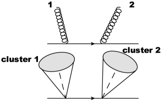
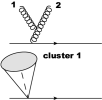
Figure 1: Example of decomposition into correlated clusters for emissions off a quark line. The left configuration corresponds to the emission of two independent gluons, and it is mapped onto two separate clusters. The right configuration corresponds to the emission of the second gluon off the first one, and it is mapped onto a single cluster. The correlated clusters are not to be confused with partonic jets.

The formulation that led to eq. (32) is based on an organisation of the perturbative series that aims at the resummation of the logarithmic terms to all orders. In particular, each evolution step in eq. (32) describes the emission of an inclusive correlated cluster of emissions Bizon:2017rah . In an illustrative picture, it is convenient to think of each inclusive cluster as describing the emission of an initial-state radiation and its subsequent branchings. The cluster is defined by integrating inclusively over the branching variables and retaining only the information about the total transverse momentum of the radiation emitted within. An illustrative example of the separation into correlated clusters for two typical configurations is reported in fig. 1.

In a slightly more technical picture, limiting ourselves to the ${\cal O}(\alpha_{s}^{2})$ case we are interested in, the correlated clusters originate from the fact that, in the soft limit, the squared amplitude for the emission of up to $2$ partons can be decomposed as

$$\left|{\cal M}(k_{1})\right|^{2} \equiv\tilde{\cal M}^{2}(k_{1})\,,$$

$$\left|{\cal M}(k_{1},k_{2})\right|^{2} =\tilde{\cal M}^{2}(k_{1})\tilde{\cal M}^{2}(k_{2})+\tilde{\cal M}^{2}(k_{1},k_{2})\,.$$ (46)

The term $\tilde{\cal M}^{2}(k_{1},k_{2})$ is defined as the correlated part of the squared amplitude that cannot be decomposed as the product of two squared amplitudes for the emission of a single parton. We point out that, in the collinear limit, a decomposition of the type (4) requires keeping track of all the possible flavour structures of a $1\to 3$ collinear branching. Each of the correlated terms $\tilde{\cal M}^{2}$ admits a perturbative expansion in powers of $\alpha_{s}$ defined by including the virtual corrections while keeping the number of emissions fixed. The inclusive correlated cluster is defined as

$${\cal M}_{\rm incl}^{2}(k)= \,{\cal M}^{2}(k)$$ (47)

$$+\,\int[dk_{a}][dk_{b}]\tilde{\cal M}^{2}(k_{a},k_{b})\delta^{(2)}(\vec{k}_{ta}+\vec{k}_{tb}-\vec{k}_{t})\delta(Y_{ab}-Y)+{\cal O}(\alpha_{s}^{3})\,,$$

$Y_{ab}$ denotes the rapidity of the $k_{a}+k_{b}$ system in the centre-of-mass frame of the collision, and $[dk]$ denotes the phase-space measure for the emission $k$. Moreover, the strong coupling constant in eq. (47) is evaluated at the transverse momentum of the inclusive cluster. For an inclusive observable such as ${p_{\text{T}}}$, the only quantity that matters is the total transverse momentum of each inclusive cluster. Therefore, one can integrate over the rapidity of each cluster, and analytically cancel the infrared and collinear singularities. This results in a simplified picture, in which each inclusive cluster of transverse momentum $k_{\scaleto{\rm T}{4pt},i}$ is emitted according to the kernel

$$S^{\prime}(k_{\scaleto{\rm T}{4pt},i})\,\mathbb{1} +\frac{\alpha_{s}(k_{\scaleto{\rm T}{4pt},i})}{\pi}\hat{P}+2\beta(\alpha_{s}(k_{\scaleto{\rm T}{4pt},i}))\frac{\mathrm{d}\ln C}{\mathrm{d}\alpha_{s}}\,,$$ (48)

and analogously for the term involving the $G$ coefficient function. In eq. (48) we implicitly sum over the two initial-state legs $a$ and $b$, and we observe that the first two terms start at order ${\cal O}(\alpha_{s})$, while the third term proportional to $\beta(\alpha_{s})$, defined in eq. (90), starts at ${\cal O}(\alpha_{s}^{2})$.

Equation (32) describes the emission of two subsequent clusters with transverse momenta $k_{\scaleto{\rm T}{4pt},1}$ and $k_{\scaleto{\rm T}{4pt},2}\leq k_{\scaleto{\rm T}{4pt},1}$. The first line of eq. (32) encodes the emission of the first cluster, while the remaining lines describe the emission of the second one. The latter is split into a no-emission probability term (that excludes configurations with more than one cluster), and a term proportional to the real kernel (48) that actually describes the second emission. We stress that, in the present treatment, we are not interested in retaining a given logarithmic accuracy in the ${p_{\text{T}}}$ spectrum, but rather in describing the correct singular structure at ${\cal O}(\alpha_{s}^{2})$. However, one should bear in mind that the evolution beyond the second emission will be subsequently generated by a parton shower generator, which will guarantee a fully exclusive treatment of the radiation. We finally observe that the term

$$2\beta(\alpha_{s}(k_{\scaleto{\rm T}{4pt},2}))\frac{\mathrm{d}\ln C}{\mathrm{d}\alpha_{s}},$$ (49)

in the second emission’s probability contributes at most to ${\cal O}(\alpha_{s}^{3})$ and therefore can be ignored.

We now proceed by adding and subtracting $\Theta({p_{\text{T}}}-k_{\scaleto{\rm T}{4pt},1})$ to the second $\Theta$ function in eq. (32) as

$$\Theta({p_{\text{T}}}-|\vec{k}_{\scaleto{\rm T}{4pt},1}+\vec{k}_{\scaleto{\rm T}{4pt},2}|) \to\Theta({p_{\text{T}}}-k_{\scaleto{\rm T}{4pt},1})$$

$$+\left(\Theta({p_{\text{T}}}-|\vec{k}_{\scaleto{\rm T}{4pt},1}+\vec{k}_{\scaleto{\rm T}{4pt},2}|)-\Theta({p_{\text{T}}}-k_{\scaleto{\rm T}{4pt},1})\right)\,.$$ (50)

We can then recast eq. (32), with ${\cal O}(\alpha_{s}^{2})$ accuracy, as

$$\frac{\mathrm{d}\sigma^{\rm sing}({p_{\text{T}}})}{\mathrm{d}\Phi_{\scriptscriptstyle\rm F}} =\int\langle\mathrm{d}k_{1}\rangle e^{-S(k_{\scaleto{\rm T}{4pt},1})}\left[S^{\prime}(k_{\scaleto{\rm T}{4pt},1})\,\mathbb{1}+\frac{\alpha_{s}(k_{\scaleto{\rm T}{4pt},1})}{\pi}\hat{P}+2\beta(\alpha_{s}(k_{\scaleto{\rm T}{4pt},1}))\frac{\mathrm{d}\ln C}{\mathrm{d}\alpha_{s}}\right]$$

$$\otimes\bigg{\{}\Delta^{(C)}(k_{\scaleto{\rm T}{4pt},1},\Lambda){\cal L}^{(C)}(k_{\scaleto{\rm T}{4pt},1})+\int\langle\mathrm{d}k_{2}\rangle\left[S^{\prime}(k_{\scaleto{\rm T}{4pt},2})\,\mathbb{1}+\frac{\alpha_{s}(k_{\scaleto{\rm T}{4pt},2})}{\pi}\hat{P}\right]\Theta(k_{\scaleto{\rm T}{4pt},1}-k_{\scaleto{\rm T}{4pt},2})$$

$$\otimes\left(\Delta^{(C)}(k_{\scaleto{\rm T}{4pt},1},k_{\scaleto{\rm T}{4pt},2}){\cal L}^{(C)}(k_{\scaleto{\rm T}{4pt},1})\right)\bigg{\}}\Theta({p_{\text{T}}}-k_{\scaleto{\rm T}{4pt},1})$$

$$+\int\langle\mathrm{d}k_{1}\rangle\int\langle\mathrm{d}k_{2}\rangle\Theta(k_{\scaleto{\rm T}{4pt},1}-k_{\scaleto{\rm T}{4pt},2})$$

$$\times\bigg{\{}S^{\prime}(k_{\scaleto{\rm T}{4pt},1})S^{\prime}(k_{\scaleto{\rm T}{4pt},2}){\cal L}^{(C)}(k_{\scaleto{\rm T}{4pt},2})+S^{\prime}(k_{\scaleto{\rm T}{4pt},1})\frac{\alpha_{s}(k_{\scaleto{\rm T}{4pt},2})}{\pi}\hat{P}\otimes{\cal L}^{(C)}(k_{\scaleto{\rm T}{4pt},2})$$

$$+S^{\prime}(k_{\scaleto{\rm T}{4pt},2})\frac{\alpha_{s}(k_{\scaleto{\rm T}{4pt},1})}{\pi}\hat{P}\otimes{\cal L}^{(C)}(k_{\scaleto{\rm T}{4pt},2})+\frac{\alpha_{s}(k_{\scaleto{\rm T}{4pt},1})}{\pi}\frac{\alpha_{s}(k_{\scaleto{\rm T}{4pt},2})}{\pi}\hat{P}\otimes\hat{P}\otimes{\cal L}^{(C)}(k_{\scaleto{\rm T}{4pt},2})\bigg{\}}$$

$$\times\left(\Theta({p_{\text{T}}}-|\vec{k}_{\scaleto{\rm T}{4pt},1}+\vec{k}_{\scaleto{\rm T}{4pt},2}|)-\Theta({p_{\text{T}}}-k_{\scaleto{\rm T}{4pt},1})\right)+{\cal O}(\alpha^{3}_{s})\,,$$ (51)

where we neglected the Sudakov form factors in the integral containing the difference between the two $\Theta$ functions, as the first non-trivial contribution generates ${\cal O}(\alpha_{s}^{3})$ corrections. The resulting integral is finite at fixed ${p_{\text{T}}}$. In order to evaluate such an integral, and since we are only interested in the ${\cal O}(\alpha_{s}^{2})$ result, we can expand the content of the curly brackets about $k_{\scaleto{\rm T}{4pt},1}={p_{\text{T}}}$ and $k_{\scaleto{\rm T}{4pt},2}={p_{\text{T}}}$ as follows

$$\bigg{\{}S^{\prime}(k_{\scaleto{\rm T}{4pt},1})S^{\prime}(k_{\scaleto{\rm T}{4pt},2}){\cal L}^{(C)}(k_{\scaleto{\rm T}{4pt},2})+S^{\prime}(k_{\scaleto{\rm T}{4pt},1})\frac{\alpha_{s}(k_{\scaleto{\rm T}{4pt},2})}{\pi}\hat{P}\otimes{\cal L}^{(C)}(k_{\scaleto{\rm T}{4pt},2})$$

$$+S^{\prime}(k_{\scaleto{\rm T}{4pt},2})\frac{\alpha_{s}(k_{\scaleto{\rm T}{4pt},1})}{\pi}\hat{P}\otimes{\cal L}^{(C)}(k_{\scaleto{\rm T}{4pt},2})+\frac{\alpha_{s}(k_{\scaleto{\rm T}{4pt},1})}{\pi}\frac{\alpha_{s}(k_{\scaleto{\rm T}{4pt},2})}{\pi}\hat{P}\otimes\hat{P}\otimes{\cal L}^{(C)}(k_{\scaleto{\rm T}{4pt},2})\bigg{\}}$$

$$=\bigg{\{}S^{\prime}({p_{\text{T}}})S^{\prime}({p_{\text{T}}}){\cal L}^{(C)}({p_{\text{T}}})+S^{\prime}({p_{\text{T}}})\frac{\alpha_{s}({p_{\text{T}}})}{\pi}\hat{P}\otimes{\cal L}^{(C)}({p_{\text{T}}})$$

$$+S^{\prime}({p_{\text{T}}})\frac{\alpha_{s}({p_{\text{T}}})}{\pi}\hat{P}\otimes{\cal L}^{(C)}({p_{\text{T}}})+\frac{\alpha_{s}({p_{\text{T}}})}{\pi}\frac{\alpha_{s}({p_{\text{T}}})}{\pi}\hat{P}\otimes\hat{P}\otimes{\cal L}^{(C)}({p_{\text{T}}})\bigg{\}}$$

$$+\bigg{\{}S^{\prime}({p_{\text{T}}})S^{\prime\prime}({p_{\text{T}}}){\cal L}^{(C)}({p_{\text{T}}})+\frac{\alpha_{s}({p_{\text{T}}})}{\pi}S^{\prime\prime}({p_{\text{T}}})\hat{P}\otimes{\cal L}^{(C)}({p_{\text{T}}})\bigg{\}}\left(\ln\frac{{p_{\text{T}}}}{k_{\scaleto{\rm T}{4pt},1}}+\ln\frac{{p_{\text{T}}}}{k_{\scaleto{\rm T}{4pt},2}}\right)$$

$$+{\cal O}(\alpha_{s}^{3})\,.$$ (52)

When performing the integration, we notice that the first term on the right-hand side of the above equation vanishes upon azimuthal integration, and we are left with the integral of the second term, obtaining

$$\frac{\mathrm{d}\sigma^{\rm sing}({p_{\text{T}}})}{\mathrm{d}\Phi_{\scriptscriptstyle\rm F}} =\int\langle\mathrm{d}k_{1}\rangle e^{-S(k_{\scaleto{\rm T}{4pt},1})}\left[S^{\prime}(k_{\scaleto{\rm T}{4pt},1})\,\mathbb{1}+\frac{\alpha_{s}(k_{\scaleto{\rm T}{4pt},1})}{\pi}\hat{P}+2\beta(\alpha_{s}(k_{\scaleto{\rm T}{4pt},1}))\frac{\mathrm{d}\ln C}{\mathrm{d}\alpha_{s}}\right]$$

$$\otimes\bigg{\{}\Delta^{(C)}(k_{\scaleto{\rm T}{4pt},1},\Lambda){\cal L}^{(C)}(k_{\scaleto{\rm T}{4pt},1})+\int\langle\mathrm{d}k_{2}\rangle\left[S^{\prime}(k_{\scaleto{\rm T}{4pt},2})\,\mathbb{1}+\frac{\alpha_{s}(k_{\scaleto{\rm T}{4pt},2})}{\pi}\hat{P}\right]\Theta(k_{\scaleto{\rm T}{4pt},1}-k_{\scaleto{\rm T}{4pt},2})$$

$$\otimes\left(\Delta^{(C)}(k_{\scaleto{\rm T}{4pt},1},k_{\scaleto{\rm T}{4pt},2}){\cal L}^{(C)}(k_{\scaleto{\rm T}{4pt},1})\right)\bigg{\}}\Theta({p_{\text{T}}}-k_{\scaleto{\rm T}{4pt},1})$$

$$-\frac{\zeta_{3}}{4}\left(S^{\prime}({p_{\text{T}}})S^{\prime\prime}({p_{\text{T}}}){\cal L}^{(C)}({p_{\text{T}}})+\frac{\alpha_{s}({p_{\text{T}}})}{\pi}S^{\prime\prime}({p_{\text{T}}})\hat{P}\otimes{\cal L}^{(C)}({p_{\text{T}}})\right)+{\cal O}(\alpha^{3}_{s})\,,$$ (53)

where $S^{\prime\prime}({p_{\text{T}}})=\mathrm{d}S^{\prime}({p_{\text{T}}})/\mathrm{d}L$.

We now incorporate the terms generated by the latter integration into the first term of eq. (53). Retaining ${\cal O}(\alpha_{s}^{2})$ accuracy, this can be done by redefining some of the resummation coefficients as follows (an alternative derivation of such redefinitions is performed using an impact-parameter space formulation in appendix E)

$$B^{(2)} \to B^{(2)}+2\zeta_{3}(A^{(1)})^{2},$$

$$H^{(2)} \to H^{(2)}-2\zeta_{3}A^{(1)}B^{(1)},$$

$$C^{(2)}(z) \to C^{(2)}(z)-2\zeta_{3}A^{(1)}\hat{P}^{(0)}(z)\,.$$ (54)

In order to use eq. (53) in the context of the MiNLO^′ algorithm, we perform a resummation-scheme transformation to evaluate the virtual corrections (44) that appear in ${\cal L}^{(C)}(k_{\scaleto{\rm T}{4pt},1})$ (41) at a scale $k_{\scaleto{\rm T}{4pt},1}$. This implies the further replacements Hamilton:2012rf

$$H(Q) \rightarrow H(k_{\scaleto{\rm T}{4pt},1})\,,$$

$$B^{(2)} \rightarrow B^{(2)}+2\pi\beta_{0}H^{(1)}\,.$$ (55)

We thus define

$$B^{(2)}\to \,\tilde{B}^{(2)}=B^{(2)}+2\zeta_{3}(A^{(1)})^{2}+2\pi\beta_{0}H^{(1)},$$

$$H^{(2)}\to \,\tilde{H}^{(2)}=H^{(2)}-2\zeta_{3}A^{(1)}B^{(1)},$$

$$C^{(2)}(z)\to \,\tilde{C}^{(2)}(z)=C^{(2)}(z)-2\zeta_{3}A^{(1)}\hat{P}^{(0)}(z)\,,$$ (56)

and we redefine all ingredients in our calculation as $S\to\tilde{S}$, $\Delta^{(C)}\to\tilde{\Delta}^{(C)}$, $C\to\tilde{C}$, and ${\cal L}^{(C)}\to{\cal\tilde{L}}^{(C)}$ to take the above replacements into account. We therefore recast eq. (53) as

$$\frac{\mathrm{d}\sigma^{\rm sing}({p_{\text{T}}})}{\mathrm{d}\Phi_{\scriptscriptstyle\rm F}} =\int\langle\mathrm{d}k_{1}\rangle e^{-\tilde{S}(k_{\scaleto{\rm T}{4pt},1})}\left[\tilde{S}^{\prime}(k_{\scaleto{\rm T}{4pt},1})\,\mathbb{1}+\frac{\alpha_{s}(k_{\scaleto{\rm T}{4pt},1})}{\pi}\hat{P}+2\beta(\alpha_{s}(k_{\scaleto{\rm T}{4pt},1}))\frac{\mathrm{d}\ln\tilde{C}}{\mathrm{d}\alpha_{s}}\right]$$

$$\otimes\bigg{\{}\tilde{\Delta}^{(C)}(k_{\scaleto{\rm T}{4pt},1},\Lambda){\cal\tilde{L}}^{(C)}(k_{\scaleto{\rm T}{4pt},1})+\int\langle\mathrm{d}k_{2}\rangle\left[\tilde{S}^{\prime}(k_{\scaleto{\rm T}{4pt},2})\,\mathbb{1}+\frac{\alpha_{s}(k_{\scaleto{\rm T}{4pt},2})}{\pi}\hat{P}\right]\Theta(k_{\scaleto{\rm T}{4pt},1}-k_{\scaleto{\rm T}{4pt},2})$$

$$\otimes\left(\tilde{\Delta}^{(C)}(k_{\scaleto{\rm T}{4pt},1},k_{\scaleto{\rm T}{4pt},2}){\cal\tilde{L}}^{(C)}(k_{\scaleto{\rm T}{4pt},1})\right)\bigg{\}}\Theta({p_{\text{T}}}-k_{\scaleto{\rm T}{4pt},1})+{\cal O}(\alpha^{3}_{s})\,.$$ (57)

Finally, we take the derivative in ${p_{\text{T}}}$ in order to obtain the singular structure of the differential ${p_{\text{T}}}$ distribution, that reads

$$\frac{\mathrm{d}\sigma^{\rm sing}}{\mathrm{d}\Phi_{\scriptscriptstyle\rm F}\mathrm{d}{p_{\text{T}}}} =\int\langle\mathrm{d}k_{1}\rangle e^{-\tilde{S}(k_{\scaleto{\rm T}{4pt},1})}\left[\tilde{S}^{\prime}(k_{\scaleto{\rm T}{4pt},1})\,\mathbb{1}+\frac{\alpha_{s}(k_{\scaleto{\rm T}{4pt},1})}{\pi}\hat{P}+2\beta(\alpha_{s}(k_{\scaleto{\rm T}{4pt},1}))\frac{\mathrm{d}\ln\tilde{C}}{\mathrm{d}\alpha_{s}}\right]$$

$$\otimes\bigg{\{}\tilde{\Delta}^{(C)}(k_{\scaleto{\rm T}{4pt},1},\Lambda){\cal\tilde{L}}^{(C)}(k_{\scaleto{\rm T}{4pt},1})+\int\langle\mathrm{d}k_{2}\rangle\left[\tilde{S}^{\prime}(k_{\scaleto{\rm T}{4pt},2})\,\mathbb{1}+\frac{\alpha_{s}(k_{\scaleto{\rm T}{4pt},2})}{\pi}\hat{P}\right]\Theta(k_{\scaleto{\rm T}{4pt},1}-k_{\scaleto{\rm T}{4pt},2})$$

$$\otimes\left(\tilde{\Delta}^{(C)}(k_{\scaleto{\rm T}{4pt},1},k_{\scaleto{\rm T}{4pt},2}){\cal\tilde{L}}^{(C)}(k_{\scaleto{\rm T}{4pt},1})\right)\bigg{\}}\delta({p_{\text{T}}}-k_{\scaleto{\rm T}{4pt},1})+{\cal O}(\alpha^{3}_{s})\,.$$ (58)

In order to be accurate across the whole ${p_{\text{T}}}$ spectrum, we need to match eq. (58) to the NLO differential cross section for the production of the colour-singlet system in association with one jet. This can be performed in two steps.

The first step is to observe that the second emission is distributed in a way that closely mimics the treatment of the radiation in the POWHEG method Nason:2004rx discussed in section 2.1, that is generated according to the probability

$$\Delta_{\rm pwg}(\Lambda_{\rm pwg})+\int\mathrm{d}\Phi_{\operatorname{rad}}\Delta_{\rm pwg}({p_{\text{T,rad}}})\frac{R(\Phi_{\scriptscriptstyle\rm FJ}{},\Phi_{\operatorname{rad}})}{B(\Phi_{\scriptscriptstyle\rm FJ}{})}\,,$$ (59)

where the factor $\Phi_{\operatorname{rad}}$ represents the full FKS Frixione:1995ms radiation phase space for the second emission $k_{2}$. The quantities $R$ and $B$ represent the tree-level squared amplitudes for ${\rm FJJ}$ (double emission) and ${\rm FJ}$ (single emission), respectively. Therefore, the second emission can be directly generated according to the POWHEG method, which guarantees an accurate description at tree level for $k_{2}$ over the whole radiation phase space $\Phi_{\operatorname{rad}}$.

We can then focus on the first cluster contribution. For simplicity we can integrate eq. (58) explicitly over the second emission $k_{2}$, stressing that the latter can be restored fully differentially by closely following the POWHEG procedure as previously discussed. We obtain

$$\frac{\mathrm{d}\sigma^{\rm sing}}{\mathrm{d}\Phi_{\scriptscriptstyle\rm F}\mathrm{d}{p_{\text{T}}}} =e^{-\tilde{S}({p_{\text{T}}})}\left[\tilde{S}^{\prime}({p_{\text{T}}})\,\mathbb{1}+\frac{\alpha_{s}({p_{\text{T}}})}{\pi}\hat{P}+2\beta(\alpha_{s}({p_{\text{T}}}))\frac{\mathrm{d}\ln\tilde{C}}{\mathrm{d}\alpha_{s}}\right]\otimes{\cal\tilde{L}}^{(C)}({p_{\text{T}}})+{\cal O}(\alpha^{3}_{s}(Q))$$

$$=\frac{\mathrm{d}\left[e^{-\tilde{S}({p_{\text{T}}})}{\cal\tilde{L}}^{(C)}({p_{\text{T}}})\right]}{\mathrm{d}{p_{\text{T}}}}+{\cal O}(\alpha^{3}_{s})\,,$$ (60)

where in the second line we recast the result in a more compact form. We can at last restore the contribution of the $G$ coefficient functions by replacing ${\cal\tilde{L}}^{(C)}$ with the full luminosity factor as

$${\cal\tilde{L}}^{(C)}(k_{\scaleto{\rm T}{4pt},1})\to{\cal L}(k_{\scaleto{\rm T}{4pt},1}) =\sum_{c,c^{\prime}}\frac{\mathrm{d}|M^{\scriptscriptstyle\rm F}|_{cc^{\prime}}^{2}}{\mathrm{d}\Phi_{\scriptscriptstyle\rm F}}\sum_{i,j}\bigg{\{}\left(\tilde{C}^{[a]}_{ci}\otimes f_{i}^{[a]}\right)\tilde{H}(k_{\scaleto{\rm T}{4pt},1})\left(\tilde{C}^{[b]}_{c^{\prime}j}\otimes f_{j}^{[b]}\right)$$

$$+\left(G^{[a]}_{ci}\otimes f_{i}^{[a]}\right)\tilde{H}(k_{\scaleto{\rm T}{4pt},1})\left(G^{[b]}_{c^{\prime}j}\otimes f_{j}^{[b]}\right)\bigg{\}}\,.$$ (61)

Equation (60), when expanded, correctly reproduces up to ${\cal O}(\alpha_{s}^{2})$ the divergent (logarithmic) structure of the differential spectrum in the small ${p_{\text{T}}}$ limit. However, eq. (60) does not yet include the regular terms in the ${p_{\text{T}}}$ distribution (i.e. those which vanish in the ${p_{\text{T}}}\to 0$ limit).

The second step to include the regular terms (i.e. that vanish in the ${p_{\text{T}}}\to 0$ limit) in the above formula is to add the full NLO result for the production of the colour singlet ${\rm F}$ and one additional jet, and subtract the NLO expansion of the total derivative in eq. (60), which leads to

$$\frac{\mathrm{d}\sigma}{\mathrm{d}\Phi_{\scriptscriptstyle\rm F}\mathrm{d}{p_{\text{T}}}}=\frac{\mathrm{d}\left[e^{-\tilde{S}({p_{\text{T}}})}{\cal L}({p_{\text{T}}})\right]}{\mathrm{d}{p_{\text{T}}}}+R_{f}({p_{\text{T}}})+{\cal O}(\alpha^{3}_{s})\,,$$ (62)

where we used eq. (14), namely

$$R_{f}({p_{\text{T}}})=\frac{\mathrm{d}\sigma^{\rm(NLO)}_{\scriptscriptstyle\rm FJ}}{\mathrm{d}\Phi_{\scriptscriptstyle\rm F}\mathrm{d}{p_{\text{T}}}}-\frac{\alpha_{s}({p_{\text{T}}})}{2\pi}\left[\frac{\mathrm{d}\sigma^{\rm sing}}{\mathrm{d}\Phi_{\scriptscriptstyle\rm F}\mathrm{d}{p_{\text{T}}}}\right]^{(1)}-\left(\frac{\alpha_{s}({p_{\text{T}}})}{2\pi}\right)^{2}\left[\frac{\mathrm{d}\sigma^{\rm sing}}{\mathrm{d}\Phi_{\scriptscriptstyle\rm F}\mathrm{d}{p_{\text{T}}}}\right]^{(2)}\,.$$ (63)

The first term on the right-hand side of eq. (62) constitutes the starting point (7) for the discussion in section 2.3. In particular, following the considerations that led from eq. (7) to eq. (28), and restoring the generation of the second radiation via the POWHEG mechanism we obtain

$$\frac{\mathrm{d}\sigma}{\mathrm{d}\Phi_{\scriptscriptstyle\rm FJ}}= \exp[-\tilde{S}({p_{\text{T}}})]\bigg{\{}\frac{\alpha_{s}({p_{\text{T}}})}{2\pi}\left[\frac{\mathrm{d}\sigma_{\scriptscriptstyle\rm FJ}}{\mathrm{d}\Phi_{\scriptscriptstyle\rm FJ}}\right]^{(1)}\left(1+\frac{\alpha_{s}({p_{\text{T}}})}{2\pi}[\tilde{S}({p_{\text{T}}})]^{(1)}\right)$$

$$+\left(\frac{\alpha_{s}({p_{\text{T}}})}{2\pi}\right)^{2}\left[\frac{\mathrm{d}\sigma_{\scriptscriptstyle\rm FJ}}{\mathrm{d}\Phi_{\scriptscriptstyle\rm FJ}}\right]^{(2)}+\left(\frac{\alpha_{s}({p_{\text{T}}})}{2\pi}\right)^{3}[D({p_{\text{T}}})]^{(3)}F^{\operatorname{corr}}(\Phi_{\scriptscriptstyle\rm FJ})\bigg{\}}$$

$$\times\bigg{\{}\Delta_{\rm pwg}(\Lambda_{\rm pwg})+\int\mathrm{d}\Phi_{\operatorname{rad}}\Delta_{\rm pwg}({p_{\text{T,rad}}})\frac{R(\Phi_{\scriptscriptstyle\rm FJ}{},\Phi_{\operatorname{rad}})}{B(\Phi_{\scriptscriptstyle\rm FJ}{})}\bigg{\}}+{\cal O}(\alpha^{3}_{s})\,,$$ (64)

where ${p_{\text{T}}}$ is defined in the $\Phi_{\scriptscriptstyle\rm FJ}$ phase space. Equation (64) constitutes the master formula for the MiNNLO_PS method, to match a fully differential NNLO calculation to a parton shower.

The NNLO subtraction in eq. (64) is accomplished thanks to the Sudakov form factor that exponentially suppresses the ${p_{\text{T}}}\to 0$ limit. We stress that this fact does not imply that the transverse-momentum spectrum of the colour singlet will be exponentially suppressed at small ${p_{\text{T}}}$. The extra emissions beyond the second one, generated by the parton shower, will eventually modify the scaling of the transverse-momentum distribution and restore the correct ${\cal O}({p_{\text{T}}})$ scaling in this regime Parisi:1979se ; Bizon:2017rah . This, for sufficiently accurate parton showers ordered in transverse momentum, effectively corresponds to leading logarithmic accuracy in the ${p_{\text{T}}}$ spectrum.

5 Application to Higgs-boson and Drell-Yan production at the LHC

In this section we apply the MiNNLO_PS method to hadronic Higgs-boson production through gluon fusion in the approximation of an infinitely heavy top quark ($pp\rightarrow H$), and to the Drell-Yan (DY) process ($pp\rightarrow Z\rightarrow\ell^{+}\ell^{-}$) for an on-shell $Z$ boson. Rather than presenting an extensive phenomenological study for these two processes at the LHC, our goal is to perform a thorough validation and numerically demonstrate the NNLO+PS accuracy of the MiNNLO_PS formula. This requires us to verify two aspects of the results: firstly, that NNLO accuracy is reached for Born-level ($\Phi_{\scriptscriptstyle\rm F}{}$) observables, in particular for the total inclusive cross section and for distributions in the Born phase space, such as the rapidity distribution of the colour-neutral boson or, in case of DY, the leptonic variables. Secondly, it has to be shown that the NLO accuracy of one-jet ($\Phi_{\scriptscriptstyle\rm FJ}$) observables is preserved, in particular for distributions related to the leading jet. To this end, we compare our MiNNLO_PS results to MiNLO^′ and to NNLO predictions. We stress that the results produced by the MiNNLO_PS method differ from the previous NNLOPS Hamilton:2013fea ; Karlberg:2014qua by higher-order terms. In particular, the latter agree by construction with the full NNLO for Born variables, therefore we validate our results by directly comparing to the nominal NNLO. After defining the general setup, we discuss the validation in the following.

5.1 Setup

We consider 13 TeV LHC collisions. For the EW parameters we employ the $G_{\mu}$ scheme with real $Z$ and $W$ masses, since we consider on-shell $Z$ bosons. Thus, the EW mixing angles are given by $\cos^{2}\theta_{\tiny{\mbox{W}}}={m_{\text{W}}}{}^{2}/{m_{\text{Z}}}{}^{2}$ and $\alpha=\sqrt{2}\,G_{\mu}{m_{\text{W}}}{}^{2}\sin^{2}\theta_{\tiny{\mbox{W}}}/\pi$. The following values are used as input parameters: $G_{\tiny{\mbox{F}}}=1.16639\times 10^{-5}$ GeV^-2, ${m_{\text{W}}}{}=80.385$ GeV, ${m_{\text{Z}}}{}=91.1876$ GeV, and ${m_{\text{H}}}{}=125$ GeV. We obtain a branching fraction of $\textrm{BR}(Z\rightarrow\ell^{+}\ell^{-})=0.0336310$ from these inputs for the $Z$-boson decay into massless leptons. With an on-shell top-quark mass of ${m_{\text{t}}}=172.5$ GeV and $n_{f}=5$ massless quark flavours, we use the corresponding NNLO PDF set with $\alpha_{s}({m_{\text{Z}}}{})=0.118$ of PDF4LHC15 Butterworth:2015oua for Higgs-boson production and of NNPDF3.0 Ball:2014uwa for the DY results.

For MiNLO^′ and MiNNLO_PS, the factorisation scale (${\mu_{\text{F}}}{}$) and renormalisation scale (${\mu_{\text{R}}}{}$) are determined by the underlying formalism to be proportional to the transverse momentum of the colour singlet, as discussed in section 2. Upon integration over radiation this corresponds to effective scales (${\mu_{\text{R}}},\,{\mu_{\text{F}}}$) of the order of ${m_{\text{H}}}{}$ and ${m_{\text{Z}}}{}$ for Higgs-boson and DY production, respectively. The latter scales are used to obtain the fixed-order results. We stress that the MiNLO^′ and MiNNLO_PS methods adopt a dynamical scale during the phase-space integration. As a consequence, the correspondence between such scales and those used in the fixed-order predictions presented below is only approximate, and for this reason one does not expect a perfect agreement between the two calculations.

Uncertainties from missing higher-order contributions are estimated from customary $7$-point variations, i.e. through changing the scales by a factor of two around their central values ${\mu_{\text{F}}}{}=K_{\text{F}}{}\,{p_{\text{T}}}$, ${\mu_{\text{R}}}{}=K_{\text{R}}{}\,{p_{\text{T}}}$ (${\mu_{\text{F}}}{}=K_{\text{F}}{}\,M$, ${\mu_{\text{R}}}{}=K_{\text{R}}{}\,M$ with $M={m_{\text{H}}}$ or $M={m_{\text{Z}}}$ for the fixed-order results) while requiring $0.5\leq K_{\text{F}}{}/K_{\text{R}}{}\leq 2$. This implies taking the minimum and maximum values of the cross section for variations $(K_{\text{F}}{},K_{\text{R}}{})=(2,2)$, $(2,1)$, $(1,2)$, $(1,1)$, $(1,\tfrac{1}{2})$, $(\tfrac{1}{2},1)$, $(\tfrac{1}{2},\tfrac{1}{2})$. The formulae for the scale variation are reported in appendix D.

When the scales ${\mu_{\text{R}}}{}$ (${\mu_{\text{F}}}{}$) are too small, we freeze them consistently everywhere, both as arguments of the strong coupling constant and partons densities, and in the terms of the cross section that depend explicitly on them. Our choice for the freezing scale is $1.8$ GeV for Drell-Yan, and $2.5$ GeV for Higgs-boson production. The choice of these freezing scales is determined from two opposite requirements: one is to stay above the lower bound of the PDF parametrization (which is a scale of the order of $1$ GeV), and the other is to remain close to the region where the Sudakov form factor is negligible, in order to make sure that the contribution at the lower integration bound of the quantity defined in (7) stays indeed negligible. This allows for a larger value in the Higgs case, where the Sudakov suppression is stronger. We note that our implementation preserves scale compensation and that the transverse momentum is not affected by this procedure. We stress again that the aforementioned scales are only used to freeze the values of $\mu_{R}$ and $\mu_{F}$, and they don’t act as a cutoff on the phase space $\Phi_{\scriptscriptstyle\rm FJ}$.

We notice that, at the freezing scale, the Sudakov form factor is already quite small: in the Higgs case, already at ${p_{\text{T}}}=3$ GeV its value is $0.01$. In the Drell-Yan case, when ${p_{\text{T}}}=1.8$ GeV the value of the Sudakov form factor is $0.1$, when ${p_{\text{T}}}=1$ GeV it is $0.03$, and it reaches the value $0.01$ for ${p_{\text{T}}}=500$ MeV. We remark that, if we were to exclude from our calculation scale variation points with $K_{\text{F}}=1/2$, the freezing scale could be taken as low as $1$ GeV, which is the PDF cutoff, without a relevant change in the result, as shown in table 1.

MiNNLOPS			$pp\to H$ (on-shell)			$pp\to Z\to\ell^{+}\ell^{-}$ (on-shell)
			freezing scale	$\sigma_{\rm tot}$ [pb]		freezing scale	$\sigma_{\rm tot}$ [fb]
default			$2.5$ GeV	$36.52(2)$		$1.8$ GeV	$1849(1)$
lower freezing scale			$1.25$ GeV	$36.46(4)$		$1$ GeV	$1845(1)$

Table 1: Total inclusive cross sections for Higgs-boson production and DY production using the MiNNLO_PS calculations, for different values of the freezing scale.

Finally, we stress that the region affected by the choice of the freezing scale is at transverse momenta where non-perturbative effects start to play a role, and in a realistic simulation these effects are taken into account by the parton shower Monte Carlo and its hadronization model.

It is important to bear in mind that we implement the scale variation in all terms of eq. (64), including the Sudakov $\tilde{S}$. The latter variation is not present in a standard NNLO calculation, and therefore probes additional sources of higher-order corrections. Hence, we expect the resulting scale dependence to be moderately larger than the one of the NNLO fixed-order predictions, reflecting the additional sources of perturbative uncertainties in the MiNNLO_PS matching procedure. Although such extra sources could be avoided, we reckon that their inclusion is more appropriate to reflect the actual uncertainties of the MiNNLO_PS method.

We have employed the POWHEG-BOX framework Nason:2004rx ; Frixione:2007vw ; Alioli:2010xd to implement the MiNNLO_PS formalism for the HJ Alioli:2010qp and ZJ Campbell:2012am processes. We compare against the original MiNLO^′ calculations of refs. Hamilton:2012np ; Hamilton:2012rf . Fixed-order results (LO, NLO, NNLO) for on-shell $pp\rightarrow H$ and $pp\rightarrow Z$ production are obtained with the Matrix framework Grazzini:2017mhc . The PDFs are evaluated with the LHAPDF Buckley:2014ana package and all convolutions are handled with HOPPET Salam:2008qg . Moreover, the evaluation of polylogarithms is carried out with the hplog package Gehrmann:2001pz .

As a cross-check we have produced NNLO results for $pp\rightarrow H$ Harlander:2002wh ; Anastasiou:2002yz ; Ravindran:2003um ; Ravindran:2002dc and $pp\rightarrow Z\rightarrow\ell^{+}\ell^{-}$ Hamberg:1990np ; vanNeerven:1991gh ; Anastasiou:2003yy ; Melnikov:2006kv ; Anastasiou:2003ds also with the HNNLO Grazzini:2008tf and DYNNLO Catani:2009sm codes, which we found to be fully compatible with the Matrix predictions within their respective systematic uncertainties. For lepton-related observables we use the results from DYNNLO in our comparison. Unless otherwise stated, all results presented throughout this section are subject to no cuts in the phase space of the final-state particles. All showered results are obtained through matching to the Pythia8 parton shower Sjostrand:2014zea , and they are shown at parton level, without hadronization or underlying-event effects. Finally, the value of the parameter $p$ of the modified logarithms of eq. (29) has to be chosen such that the logarithmic terms are switched off sufficiently quickly at large transverse momentum, in order to avoid spurious effects in the region dominated by hard radiation. We adopt $p=6$ in the following, that is slightly larger than the values used in standard resummations Banfi:2012jm ; Bizon:2017rah , and verified that variations of $p$ lead to very moderate effects that are well within the quoted uncertainties.

5.2 Inclusive cross section

			$pp\to H$ (on-shell)			$pp\to Z\to\ell^{+}\ell^{-}$ (on-shell)
			$\sigma_{\rm inclusive}$ [pb]	$\sigma/\sigma_{\rm NNLO}$		$\sigma_{\rm inclusive}$ [fb]	$\sigma/\sigma_{\rm NNLO}$
LO			$12.89(0)_{-17.3\%}^{+23.5\%}$	0.325		$1658(0)_{-12.3\%}^{+11.3\%}$	0.881
NLO			$29.55(0)_{-15.3\%}^{+19.8\%}$	0.745		$1897(0)_{-4.7\%\phantom{1}}^{+3.0\%\phantom{1}}$	1.008
NNLO			$39.63(3)_{-10.4\%}^{+10.7\%}$	1.000		$1882(1)_{-0.9\%\phantom{1}}^{+1.1\%\phantom{1}}$	1.000
MiNLO′			$30.40(3)_{-15.0\%}^{+33.3\%}$	0.767		$1774(1)_{-14.8\%}^{+14.2\%}$	0.943
MiNNLOPS			$36.52(2)_{-13.4\%}^{+13.9\%}$	0.921		$1849(1)_{-2.3\%\phantom{1}}^{+1.8\%\phantom{1}}$	0.983

Table 2: Predictions of the total inclusive cross section for Higgs-boson production and the DY process at the LO, NLO, and NNLO, as well as using the MiNLO^′ and MiNNLO_PS calculations. For comparison also a column with the ratio to the NNLO cross section is shown.

We report MiNNLO_PS results for the total inclusive cross section in table 2, together with the LO, NLO, NNLO, and MiNLO^′ predictions. We start by discussing the Higgs cross sections: Compared to MiNLO^′ we find a $+19\%$ effect by including NNLO corrections through the MiNNLO_PS procedure. Furthermore, as expected from including an additional order in the perturbative series, the size of the uncertainties due to scale variations are reduced. In particular the upper variation bound is almost a factor of three smaller for MiNNLO_PS in comparison to MiNLO^′. The MiNNLO_PS and NNLO results agree well within their respective scale-uncertainty bands, which largely overlap. The central values of the two calculations differ by $7.9\%$ as can be seen from the ratio, and they are included in the uncertainty bands of each of the two calculations. The size of the difference is justified by the large perturbative corrections that characterise Higgs-boson production, which implies that subleading terms can be sizable. For processes with smaller corrections these differences will reduce, as we will see in the context of the DY process below. As already mentioned above, it is not expected that MiNNLO_PS reproduces the NNLO result exactly, as subleading corrections are treated differently in the two calculations and the the renormalisation and factorisation scales are set differently. Consistency between the two NNLO-accurate predictions within perturbative uncertainties is therefore sufficient, and shows that the MiNNLO_PS procedure induces the expected corrections. The scale uncertainties of MiNNLO_PS for the total cross section ($\sim 13\%$) are slightly larger than the NNLO ones ($\sim 10\%$). There are two main reasons for this behaviour: On the one hand, MiNNLO_PS probes scales in both the PDFs and in $\alpha_{s}{}$ that in the bulk-region of the cross section are much lower ($\sim{p_{\text{T}}}$) than in the fixed-order computation, which naturally induces a larger scale dependence. On the other hand, we include additional scale-dependent terms (as pointed out before) that originate from the analytic Sudakov form factor in the MiNNLO_PS procedure, which are absent in a fixed-order calculation, see appendix D. This induces a more conservative estimate for the theory uncertainties of the MiNNLO_PS predictions.

In the case of the DY results in table 2, we observe that conclusions similar to the case of Higgs production can be drawn, albeit with significantly smaller corrections: The effect of the MiNNLO_PS procedure is to increase the MiNLO^′ cross section by about $5\%$. Again the scale uncertainties are vastly reduced, in the case of DY by almost a factor of 10. The MiNNLO_PS result is only $1.7\%$ below the NNLO prediction and they are in good agreement within their respective scale uncertainties, which are extremely small. Roughly speaking, scale uncertainties are $2\%$ for MiNNLO_PS, which is a bit larger than the $1\%$ uncertainties at NNLO. Given the above discussion about the formal differences between MiNNLO_PS and NNLO fixed-order computations, these results are very compelling and provide a numerical proof of the accuracy of the total inclusive cross section of the MiNNLO_PS procedure. We will now turn to validating the MiNNLO_PS results also for differential observables.

5.3 Distributions for Higgs-boson production

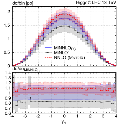
Figure 2: Distribution in the transverse momentum (left) and rapidity (right) of the Higgs boson for MiNNLO_PS (blue, solid), MiNLO^′ (black, dotted), and NNLO (red, dashed).

We first consider the case of Higgs-boson production. The figures of this section are organized as follows: the main frame shows the results from MiNNLO_PS (blue,solid) and MiNLO^′ (black, dotted) after parton showering, as well as NNLO predictions (red, dashed), and all results are reported in units of cross section per bin (namely, the sum of the values of the bins is equal to the total cross section, possibly within cuts). In an inset we display the bin-by-bin ratio of all the histograms which appear in the main frame to the MiNNLO_PS curve. The bands correspond to the residual uncertainties that are computed from scale variations as indicated in section 5.1.

The transverse-momentum distribution of the Higgs boson (${p_{\text{T,H}}}$) is shown in the left panel of figure 2. At fixed order this distribution diverges in the ${p_{\text{T,H}}}\rightarrow 0$ limit, and the accuracy is effectively reduced to NLO across the spectrum. By comparing MiNNLO_PS and MiNLO^′ curves, we observe that the NNLO corrections are included consistently in the low-${p_{\text{T,H}}}$ region through the MiNNLO_PS procedure. The additional NNLO (two-loop) contributions in the MiNNLO_PS matching are spread in a way that is similar in spirit to how analytic resummations are combined with fixed order. This is enforced through the use of the modified logarithms in eq. (29). At large ${p_{\text{T,H}}}$, where the MiNNLO_PS and MiNLO^′ predictions have both NLO accuracy, we expect the MiNNLO_PS procedure not to alter the MiNLO^′ distribution, as can be seen from the figure. The harder tail of the NNLO curve is due to the different (less appropriate) scale choice in the fixed-order calculation, set to the Higgs-boson mass rather than to ${p_{\text{T,H}}}$.

The rapidity distribution of the Higgs boson (${y_{\text{H}}}$) in the right panel of figure 2 is the most relevant observable for which MiNNLO_PS needs to be validated against the NNLO result. Indeed, we find that up to statistical fluctuations the NNLO/MiNNLO_PS ratio of the distribution is completely flat, which shows their equivalence. Henceforth, the difference of the two results is purely due to the normalisation, i.e. the total inclusive cross section, which has been discussed in detail in section 5.2 and requires no further comments. In particular, the conclusions about the uncertainty bands and the size of the corrections drawn from table 2 hold also for the rapidity distribution shown in figure 2.

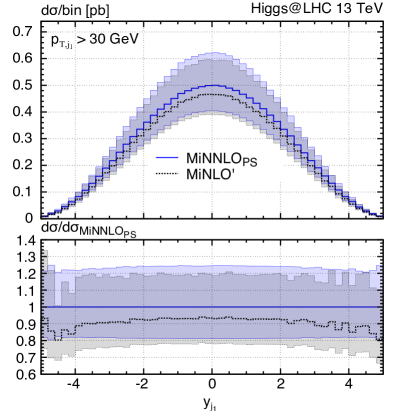
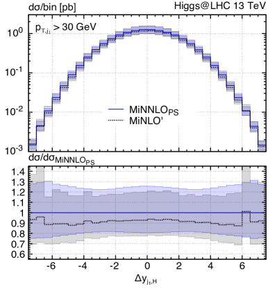
Figure 3: Distribution in the rapidity of the leading-jet (left) and its rapidity difference with the Higgs boson (right) for MiNNLO_PS (blue, solid) and MiNLO^′ (black, dotted).

We conclude our discussion of the results for Higgs-boson production by looking at jet-related distributions. We note that the transverse-momentum distribution of the leading jet is very similar to the one of the Higgs boson which is why we refrain from showing it here and refer to the discussion for ${p_{\text{T,H}}}$. Figure 3 shows the rapidity distribution of the leading jet in the left panel, and the rapidity difference between the leading jet and the Higgs boson in the right panel. Jets in this case are defined using the anti-$k_{T}$ clustering Cacciari:2008gp with a radius $R=0.4$, and a minimum transverse momentum of ${p_{\text{T,J}}}=30$ GeV. For such observables both MiNNLO_PS and MiNLO^′ are NLO accurate, and one expects that the MiNNLO_PS result does not differ from the MiNLO^′ prediction significantly, i.e. beyond perturbative uncertainties. In particular, this numerical check is important to ensure that the implementation and spreading of the $[D({p_{\text{T}}})]^{(3)}$ terms in the $\Phi_{\scriptscriptstyle\rm FJ}$ phase space, as described in section 3, is appropriate. We refrain from showing the NNLO curve for these distributions, as it does not add any relevant information to these tests. Indeed, we observe that, by and large, the MiNLO^′/MiNNLO_PS ratio is flat for both distributions in figure 3, and that the two results agree very well within perturbative uncertainties. We have repeated these checks for various ${p_{\text{T,J}}}$ thresholds in the jet definition, with the same conclusions. In particular, we found that for hard configurations (${p_{\text{T,J}}}\gtrsim 60$ GeV) the MiNNLO_PS and MiNLO^′ results become essentially identical, as expected from the fact that MiNNLO_PS induces no additional corrections in phase-space regions where the radiation is hard. Furthermore, a similar level of agreement is found also for the azimuthal angle between the leading jet and the Higgs boson.

5.4 Distributions for Drell-Yan production

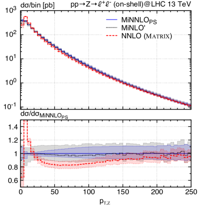
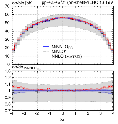
Figure 4: Distribution in the transverse momentum (left) and rapidity (right) of the $Z$ boson for MiNNLO_PS (blue, solid), MiNLO^′ (black, dotted), and NNLO (red, dashed).

We now move on to discuss distributions for the DY process. Since most of the conclusions are similar to the ones for Higgs-boson production, we keep the discussion rather brief. In addition to the results discussed for the Higgs, we also study the kinematics of the leptons arising from the decay of the $Z$ boson.

Figure 4 shows the transverse-momentum distribution of the $Z$ boson (${p_{\text{T,Z}}}$) in the left panel, and its rapidity distribution (${y_{\text{Z}}}$) in the right panel. As seen before, the corrections are smaller in the case of the DY process, but the general behaviour is the same as for Higgs-boson production: At large ${p_{\text{T,Z}}}$ the MiNNLO_PS result is essentially identical to the MiNLO^′ one, while the additional NNLO terms enter at smaller values of ${p_{\text{T,Z}}}$. The NNLO spectrum diverges at small ${p_{\text{T,Z}}}$, and is harder in the tail due to the different scale setting. For the ${y_{\text{Z}}}$ distribution, the MiNNLO_PS uncertainties are significantly reduced with respect to the MiNLO^′ ones. In the central region ($|{y_{\text{Z}}}|<3$) the NNLO/MiNNLO_PS ratio is nicely flat up to statistical fluctuations, and the two results agree within their respective uncertainties. For very forward $Z$ bosons ($|{y_{\text{Z}}}|>3$), on the other hand, we observe a slight increase of the NNLO/MiNNLO_PS ratio. We have checked explicitly that without the Pythia8 parton shower, i.e. at the level of Les Houches events, this effect is more moderate and the NNLO and MiNNLO_PS uncertainty bands overlap in the forward region. In fact, we noticed that already for the MiNLO^′ prediction, Pythia8 has the same effect, making the $Z$-boson rapidity distribution slightly more central.

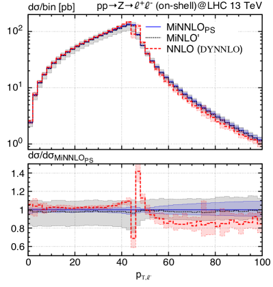
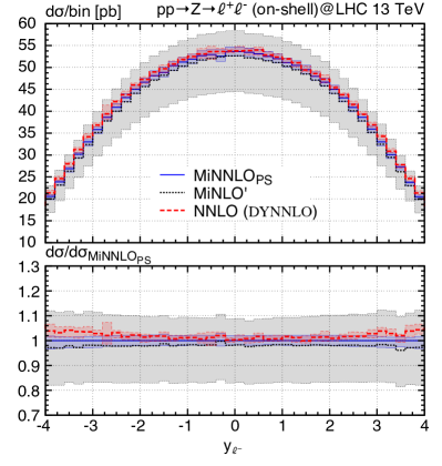
Figure 5: Distribution in the transverse momentum (left) and rapidity (right) of the negatively charged lepton for MiNNLO_PS (blue, solid), MiNLO^′ (black, dotted), and NNLO (red, dashed).

Next, we consider the transverse-momentum distribution of the negatively charged lepton (${p_{\text{T,$\ell^{-}$}}}$) and its rapidity distribution (${y_{\text{$\ell^{-}$}}}$) in the left and right panels of figure 5, respectively. For the rapidity distribution the relative behaviour between MiNNLO_PS, MiNLO^′, and NNLO is essentially identical to the one of the $Z$-boson rapidity and does not require any further discussion. As far as the transverse-momentum spectrum is concerned, the NNLO result shows a very peculiar behaviour for ${p_{\text{T,$\ell^{-}$}}}={m_{\text{Z}}}{}/2$, which reflects the perturbative instability associated with the fact that the leptons at LO are back-to-back and can share only the available partonic centre-of-mass energy $\sqrt{\hat{s}}={m_{\text{Z}}}{}$, so that their transverse momenta can be at most ${p_{\text{T,$\ell^{-}$}}}\leq{m_{\text{Z}}}{}/2$. Beyond this value the NNLO result is therefore effectively only NLO accurate, which can be also seen from the increased uncertainty band. Since such an instability is related to soft-gluon effects, this feature is cured in both the MiNNLO_PS and MiNLO^′ results, which are in good agreement with each other in terms of shape. Again the MiNNLO_PS uncertainty band is significantly smaller than the MiNLO^′ one, and we observe a rather constant correction, of the order of $\sim 5-10\%$, due to the additional NNLO terms.

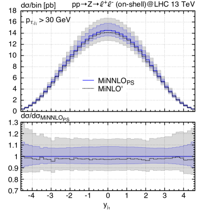
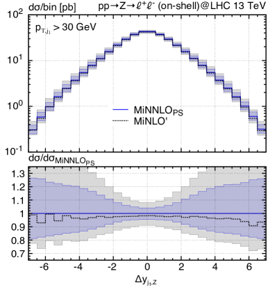
Figure 6: Distribution in the rapidity of the leading-jet (left) and its rapidity difference with the $Z$ boson (right) for MiNNLO_PS (blue, solid) and MiNLO^′ (black, dotted).

Finally, also for the DY process the jet-related observables are fully consistent within uncertainties when comparing MiNNLO_PS and MiNLO^′ predictions, as can be seen in figure 6. However, the size of their uncertainty bands is very different. This is due to the fact that in the original MiNLO^′ prediction a different prescription for the scale variation was adopted, that also involved the integration boundaries of the Sudakov form factor. We have checked that by using our prescription in MiNLO^′ the uncertainty band becomes comparable to the MiNNLO_PS one. We stress again that we have tested a variety of ${p_{\text{T,J}}}$ thresholds in the jet definition, and also looked at the azimuthal angle between the leading jet and the $Z$ boson, and found consistent results throughout.

6 Summary

In this article we have presented a novel approach, dubbed MiNNLO_PS, to combine NNLO QCD calculations with parton showers for colour-singlet production at the LHC. The method is based on the MiNLO^′ procedure, which achieves NLO accurate predictions simultaneously in the zero-jet phase space $\Phi_{\scriptscriptstyle\rm F}$ and in the one-jet phase space $\Phi_{\scriptscriptstyle\rm FJ}$. The necessary terms to achieve NNLO accuracy are derived by establishing a connection of the MiNLO^′ and POWHEG methods with the structure of transverse-momentum resummation in direct space. The consistent inclusion of these terms on top of a MiNLO^′ computation allows us to achieve NNLO+PS accuracy for a variety of collider reactions.

We have discussed in detail a suitable implementation of the NNLO corrections within the MiNLO^′ formalism, and their spreading in the $\Phi_{\scriptscriptstyle\rm FJ}$ phase space. The resulting matching preserves the leading logarithmic structure of the shower Monte Carlo for showers ordered in the transverse momentum, and the final result is NNLO accurate in the zero-jet phase space while being NLO accurate in the one-jet phase space. The combination of the two multiplicities does not require any unphysical merging scale.

As a proof of concept, we have applied the approach to hadronic Higgs production in the heavy-top limit and to the DY process, where a pair of leptons is produced via the decay of an on-shell $Z$ boson. Our results show that NNLO accuracy is reached both for the total inclusive cross section and for Born-level distributions. Differences with NNLO fixed-order results arise only from terms beyond the nominal accuracy, and the two calculations agree well for such observables within the respective perturbative uncertainties estimated from scale variations. As expected, we observe a significant reduction of the scale dependence with respect to the MiNLO^′ results, in line with the inclusion of the NNLO corrections. It was further verified that for jet-related observables in the $\Phi_{\scriptscriptstyle\rm FJ}$ phase space, where the accuracy of MiNNLO_PS and MiNLO^′ is formally identical, no significant effects are induced by the MiNNLO_PS corrections.

The algorithm is very efficient, and NNLO accuracy is achieved directly at generation time without any additional reweighting. The total MiNNLO_PS simulation requires just $50\%$ more CPU time than the usual MiNLO^′ computation. This makes it suitable for the application to more involved colour-singlet processes, such as vector-boson pair production, which is of significant phenomenological interest. A potential limitation of the algorithm concerns systems with very low invariant mass, such as low-mass diphoton production, whose ${p_{\text{T}}}{}$ distribution is peaked towards non-perturbative scales. In this situation, the Sudakov form factor, which is responsible for the NNLO subtraction of the infrared singularities, can become intrinsically non-perturbative. Nevertheless, such scenarios are commonly not of experimental interest. Finally, the MiNNLO_PS approach could be generalized to the production of massive coloured final states, such as top-quark pair production. Detailed studies of further applications of the MiNNLO_PS method are left for future work.

Appendix A Phase-space parametrisation for the $[D({p_{\text{T}}})]^{(3)}$ term

In this appendix we define the phase-space mapping from $\Phi_{\scriptscriptstyle\rm FJ}$ to $\Phi_{\scriptscriptstyle\rm F}$ adopted for initial-state radiation in POWHEG, and discussed in section 5.5.1 of ref. Frixione:2007vw . The projection is defined by performing a longitudinal boost of the ${\rm FJ}$ system to a frame where ${\rm F}$ has zero rapidity, followed by a perpendicular boost that modifies the transverse momentum of ${\rm F}$ so that it is equal to zero, followed by a longitudinal boost, exactly opposite to the first one, that restores the original rapidity of ${\rm F}$. After this sequence of boosts, the rapidity of ${\rm F}$ remains unchanged, but its transverse momentum has become zero, thus yielding a kinematic configuration in the Born phase space $\Phi_{\scriptscriptstyle\rm F}$. The $\Phi_{\scriptscriptstyle\rm FJ}$ phase space can then be expressed in a factorised form:

$$\mathrm{d}\Phi_{\scriptscriptstyle\rm FJ}=\mathrm{d}\Phi_{\scriptscriptstyle\rm F}\mathrm{d}\Phi_{\operatorname{rad}},\quad\mathrm{d}\Phi_{\operatorname{rad}}=\frac{s}{(4\pi)^{3}}\frac{\xi}{1-\xi}\mathrm{d}\xi\mathrm{d}\phi\mathrm{d}y,$$ (76)

where $s$ is the square of the total incoming energy, and

$$\xi =\frac{2k^{0}}{\sqrt{s}}, \phantom{,}k^{0} =\mbox{energy of the radiated parton,}$$ (77)

$$y =\cos\theta, \phantom{,}\theta =\mbox{scattering angle of the radiated parton,}$$ (78)

$$\phi \phantom{,}\phi =\mbox{azimuth of the radiated parton,}$$ , (79)

which are all defined in the centre-of-mass frame of the ${\rm FJ}$ system. The transverse momentum is given by

$${p_{\text{T}}}^{2}=\frac{s}{4}\xi^{2}(1-y^{2}).$$

Denoting ${\bar{\Phi}}^{\prime}_{\scriptscriptstyle\rm FJ}\equiv\left.\Phi_{\scriptscriptstyle\rm FJ}^{\prime}\right|_{\Phi_{\scriptscriptstyle\rm F}^{\prime}=\Phi_{\scriptscriptstyle\rm F}}$, the $F^{\operatorname{corr}}_{\ell}{}$ factor (22) becomes

$$F^{\operatorname{corr}}_{\ell}(\Phi_{\scriptscriptstyle\rm FJ})=\frac{J_{\ell}(\Phi_{\scriptscriptstyle\rm FJ})}{\sum_{l^{\prime}}\int\mathrm{d}\Phi^{\prime}_{\operatorname{rad}}J_{l^{\prime}}({\bar{\Phi}}^{\prime}_{\scriptscriptstyle\rm FJ})\delta({p_{\text{T}}}-{p_{\text{T}}}^{\prime})}.$$ (80)

So, we get

$$(F^{\operatorname{corr}}_{\ell}(\Phi_{\scriptscriptstyle\rm FJ}))^{-1}=J_{\ell}^{-1}(\Phi_{\scriptscriptstyle\rm FJ})\int\mathrm{d}\xi\,\mathrm{d}\phi\,\mathrm{d}y\frac{s}{(4\pi)^{3}}\frac{\xi}{1-\xi}\,J_{\ell}({\bar{\Phi}}^{\prime}_{\scriptscriptstyle\rm FJ})\,\delta\left(\sqrt{\frac{s}{4}\xi^{2}(1-y^{2})}-{p_{\text{T}}}\right).$$ (81)

We now replace $\bar{s}=s(1-\xi)$, where $\bar{s}$ is the virtuality of the ${\rm FJ}$ system, and multiply and divide by $2{p_{\text{T}}}$. After rearranging the delta function we get

$$(F^{\operatorname{corr}}_{\ell}(\Phi_{\scriptscriptstyle\rm FJ}))^{-1}=J_{\ell}^{-1}(\Phi_{\scriptscriptstyle\rm FJ})\frac{\bar{s}}{(4\pi)^{3}}\int\mathrm{d}\xi\,\mathrm{d}\phi\,\mathrm{d}y\frac{\xi}{(1-\xi)^{2}}\,J_{\ell}({\bar{\Phi}}^{\prime}_{\scriptscriptstyle\rm FJ})\,2{p_{\text{T}}}\delta\left(\frac{\bar{s}}{4}\frac{\xi^{2}(1-y^{2})}{1-\xi}-{p_{\text{T}}}^{2}\right).$$ (82)

We introduce a variable

$$t=\frac{\xi^{2}}{1-\xi}\,,$$ (83)

which is a monotonically increasing function of $\xi$ in the range $[0,\infty]$ for $\xi\in[0,1]$. We have

$$\mathrm{d}t=\frac{2\xi-\xi^{2}}{(1-\xi)^{2}}\mathrm{d}\xi,$$

and obtain

$$(F^{\operatorname{corr}}_{\ell}(\Phi_{\scriptscriptstyle\rm FJ}))^{-1} = J_{\ell}^{-1}(\Phi_{\scriptscriptstyle\rm FJ})\frac{\bar{s}}{(4\pi)^{3}}\int\mathrm{d}t\mathrm{d}\phi\mathrm{d}y\frac{(1-\xi)^{2}}{\xi(2-\xi)}\frac{\xi}{(1-\xi)^{2}}J_{\ell}({\bar{\Phi}}^{\prime}_{\scriptscriptstyle\rm FJ})2{p_{\text{T}}}\delta\left(\frac{\bar{s}}{4}t(1-y^{2})-{p_{\text{T}}}^{2}\right)$$ (84)

$$= J^{-1}_{\ell}(\Phi_{\scriptscriptstyle\rm FJ})\frac{4{p_{\text{T}}}}{(4\pi)^{2}}\int\,\mathrm{d}y\,\frac{1}{1-y^{2}}\frac{1}{2-\xi}J_{\ell}({\bar{\Phi}}^{\prime}_{\scriptscriptstyle\rm FJ})\,\Theta\left(t_{\max}(1-y^{2})-\frac{4{p_{\text{T}}}^{2}}{\bar{s}}\right)\,,$$

where

$$t=\frac{4{p_{\text{T}}}^{2}}{\bar{s}(1-y^{2})},\quad\xi=-\frac{t}{2}+\sqrt{\frac{t^{2}}{4}+t}\,,$$

  

and $t_{\max}$ is defined as the $t$ value corresponding to $\xi_{\max}$, namely

$$\xi_{\max}=1-\max\left\{\frac{2(1+y)\bar{x}_{1}^{2}}{\sqrt{(1+\bar{x}_{1}^{2})^{2}(1-y)^{2}+16y\bar{x}_{1}^{2}}+(1-y)(1-\bar{x}_{1}^{2})},(y\rightarrow-y,1\rightarrow 2)\right\}.$$

The variables $\bar{x}_{1,2}$ are the momentum fractions of the two initial-state partons in the $\Phi_{\scriptscriptstyle\rm F}$ phase space, and are defined as Frixione:2007vw

$$\bar{x}_{1}\equiv x_{1}\,\sqrt{1-\xi}\sqrt{\frac{2-\xi(1+y)}{2-\xi(1-y)}}\,,\qquad\bar{x}_{2}\equiv x_{2}\,\sqrt{1-\xi}\sqrt{\frac{2-\xi(1-y)}{2-\xi(1+y)}}\,,$$ (85)

with $x_{1,2}$ being the momentum fractions of the two initial-state partons in the $\Phi_{\scriptscriptstyle\rm FJ}$ phase space. For most choices of the function $J_{\ell}(\Phi_{\scriptscriptstyle\rm FJ})$ discussed in section 3, the above integral must be evaluated numerically via usual Monte Carlo techniques. However, for the choice $J_{\ell}(\Phi_{\scriptscriptstyle\rm FJ})=1$, we can perform the $y$ integration analytically. We need the following elementary integral

$$I(y) = \int\mathrm{d}y\frac{1}{(1-y^{2})\left(2+\frac{K}{2(1-y^{2})}-\sqrt{\frac{K}{1-y^{2}}+\frac{K^{2}}{4(1-y^{2})^{2}}}\right)}$$ (86)

$$= \frac{1}{2}\ln\left(\frac{1+y}{1-y}\right)+\frac{1}{4}\ln\frac{\sqrt{K^{-1}(1-y^{2})+\frac{1}{4}}+\frac{1}{2}+2K^{-1}(1-y)}{\sqrt{K^{-1}(1-y^{2})+\frac{1}{4}}+\frac{1}{2}+2K^{-1}(1+y)}\,.$$

The limits of integration have to be computed numerically, by finding the minimum and maximum value such that the $\Theta$ function in eq. (84) is 1. Denoting by $y_{1}$ and $y_{2}$ the lower and upper integration boundaries, respectively, we simply find that

$$(F^{\operatorname{corr}}_{\ell}(\Phi_{\scriptscriptstyle\rm FJ}))^{-1}=\frac{{p_{\text{T}}}}{4\pi^{2}}(I(y_{2})-I(y_{1}))\,.$$ (87)

Finally, we conclude this appendix by reporting the collinear approximation for $J_{\ell}(\Phi_{\scriptscriptstyle\rm FJ})$ discussed in section 3. Its expressions are taken from ref. Nason:2006hfa and adapted to the notation of this appendix. For gluon-initiated processes, the different flavour configurations read

$$J_{qg}(\Phi_{\scriptscriptstyle\rm FJ})= \,C_{F}\frac{\alpha_{s}}{2\pi}\frac{1+\xi^{2}}{(1-\xi)(1-y)\xi}f_{q}^{[a]}f_{g}^{[b]}\,,$$

$$J_{gq}(\Phi_{\scriptscriptstyle\rm FJ})= \,C_{F}\frac{\alpha_{s}}{2\pi}\frac{1+\xi^{2}}{(1-\xi)(1+y)\xi}f_{g}^{[a]}f_{q}^{[b]}\,,$$

$$J_{gg}(\Phi_{\scriptscriptstyle\rm FJ})= \,2C_{A}\frac{\alpha_{s}}{2\pi}\left[\frac{1-\xi}{\xi}+\frac{\xi}{1-\xi}+\xi(1-\xi)\right]\frac{2}{(1-y^{2})\xi}f_{g}^{[a]}f_{g}^{[b]}\,.$$ (88)

For quark-initiated reactions we have

$$J_{q\bar{q}}(\Phi_{\scriptscriptstyle\rm FJ})= \,C_{F}\frac{\alpha_{s}}{2\pi}\left[\frac{1+(1-\xi)^{2}}{\xi}\right]\frac{2}{(1-y^{2})\xi}f_{q}^{[a]}f_{\bar{q}}^{[b]}\,,$$

$$J_{qg}(\Phi_{\scriptscriptstyle\rm FJ})= \,T_{F}\frac{\alpha_{s}}{2\pi}\frac{\xi^{2}+(1-\xi)^{2}}{(1+y)\xi}f_{q}^{[a]}f_{g}^{[b]}\,,$$

$$J_{gq}(\Phi_{\scriptscriptstyle\rm FJ})= \,T_{F}\frac{\alpha_{s}}{2\pi}\frac{\xi^{2}+(1-\xi)^{2}}{(1-y)\xi}f_{g}^{[a]}f_{q}^{[b]}\,.$$ (89)

Appendix B Resummation formulae

In this section we report the expressions of the quantities appearing in the calculation of the analytic transverse-momentum spectrum that we have used throughout this article.

First of all we report our convention for the renormalisation-group equation of the strong coupling:

$$\frac{\mathrm{d}\alpha_{s}(\mu)}{\mathrm{d}\ln\mu^{2}}=\beta(\alpha_{s})\equiv-\alpha_{s}\left(\beta_{0}\alpha_{s}+\beta_{1}\alpha_{s}^{2}+\beta_{2}\alpha_{s}^{3}+\dots\right),$$ (90)

where the coefficients of the $\beta$-function are

$$\beta_{0} = \frac{11C_{A}-2n_{f}}{12\pi}\,,\qquad\beta_{1}=\frac{17C_{A}^{2}-5C_{A}n_{f}-3C_{F}n_{f}}{24\pi^{2}}\,,$$ (91)

$$\beta_{2} = \frac{2857C_{A}^{3}+(54C_{F}^{2}-615C_{F}C_{A}-1415C_{A}^{2})n_{f}+(66C_{F}+79C_{A})n_{f}^{2}}{3456\pi^{3}}\,,$$ (92)

with $C_{A}=N_{c}$, $C_{F}=\frac{N_{c}^{2}-1}{2N_{c}}$, $N_{c}=3$, and the number of light flavours $n_{f}=5$.

The Sudakov radiator $\tilde{S}({p_{\text{T}}})$ in eq. (9), with the accuracy considered in this article, can be expressed as

$$\tilde{S}({p_{\text{T}}})=-Lg_{1}(\lambda)-g_{2}(\lambda)-\frac{\alpha_{s}(Q)}{\pi}g_{3}(\lambda)\,$$ (93)

with $\lambda=\alpha_{s}(Q)\beta_{0}\ln(Q/{p_{\text{T}}})$, and

$$g_{1}(\lambda)= \frac{A^{(1)}}{\pi\beta_{0}}\frac{2\lambda+\ln(1-2\lambda)}{2\lambda},$$ (94)

$$g_{2}(\lambda)= \frac{1}{2\pi\beta_{0}}\ln(1-2\lambda)B^{(1)}-\frac{A^{(2)}}{4\pi^{2}\beta_{0}^{2}}\frac{2\lambda+(1-2\lambda)\ln(1-2\lambda)}{1-2\lambda}$$

$$-A^{(1)}\frac{\beta_{1}}{4\pi\beta_{0}^{3}}\frac{\ln(1-2\lambda)((2\lambda-1)\ln(1-2\lambda)-2)-4\lambda}{1-2\lambda}\,,$$ (95)

$$g_{3}(\lambda)= B^{(1)}\frac{\beta_{1}}{2\beta_{0}^{2}}\frac{2\lambda+\ln(1-2\lambda)}{1-2\lambda}-\frac{1}{2\pi\beta_{0}}\frac{\lambda}{1-2\lambda}\tilde{B}^{(2)}-\frac{A^{(3)}}{4\pi^{2}\beta_{0}^{2}}\frac{\lambda^{2}}{(1-2\lambda)^{2}}$$

$$+A^{(2)}\frac{\beta_{1}}{4\pi\beta_{0}^{3}}\frac{2\lambda(3\lambda-1)+(4\lambda-1)\ln(1-2\lambda)}{(1-2\lambda)^{2}}$$

$$+A^{(1)}\bigg{(}\frac{\lambda\left(\beta_{0}\beta_{2}(1-3\lambda)+\beta_{1}^{2}\lambda\right)}{\beta_{0}^{4}(1-2\lambda)^{2}}+\frac{(1-2\lambda)\ln(1-2\lambda)\left(\beta_{0}\beta_{2}(1-2\lambda)+2\beta_{1}^{2}\lambda\right)}{2\beta_{0}^{4}(1-2\lambda)^{2}}$$

$$\hskip 28.45274pt+\frac{\beta_{1}^{2}}{4\beta_{0}^{4}}\frac{(1-4\lambda)\ln^{2}(1-2\lambda)}{(1-2\lambda)^{2}}\bigg{)}\,.$$ (96)

The resummation coefficient $\tilde{B}^{(2)}$ is defined as according to eqs. (54), (55), namely

$$\tilde{B}^{(2)}= B^{(2)}+2\zeta_{3}(A^{(1)})^{2}+2\pi\beta_{0}H^{(1)}\,.$$ (97)

For Higgs-boson production in gluon fusion, the coefficients $A^{(i)}$ and $B^{(i)}$ which enter the formulae above are

$$A_{\rm ggH}^{(1)}= \;2C_{A},$$

$$\vspace{1.5mm}A_{\rm ggH}^{(2)}= \left(\frac{67}{9}-\frac{\pi^{2}}{3}\right)C_{A}^{2}-\frac{10}{9}C_{A}n_{f},$$

$$\vspace{1.5mm}A_{\rm ggH}^{(3)}= \left(-22\zeta_{3}-\frac{67\pi^{2}}{27}+\frac{11\pi^{4}}{90}+\frac{15503}{324}\right)C_{A}^{3}+\left(\frac{10\pi^{2}}{27}-\frac{2051}{162}\right)C_{A}^{2}n_{f}$$

$$+\left(4\zeta_{3}-\frac{55}{12}\right)C_{A}C_{F}n_{f}+\frac{50}{81}C_{A}n_{f}^{2},$$

$$\vspace{1.5mm}B_{\rm ggH}^{(1)}= -\frac{11}{3}C_{A}+\frac{2}{3}n_{f},$$

$$\vspace{1.5mm}B_{\rm ggH}^{(2)}= \left(\frac{11\zeta_{2}}{6}-6\zeta_{3}-\frac{16}{3}\right)C_{A}^{2}+\left(\frac{4}{3}-\frac{\zeta_{2}}{3}\right)C_{A}n_{f}+n_{f}C_{F}.$$ (98)

Similarly, for Drell-Yan production they read

$$A_{\rm DY}^{(1)}= \;2C_{F},$$

$$\vspace{1.5mm}A_{\rm DY}^{(2)}= \left(\frac{67}{9}-\frac{\pi^{2}}{3}\right)C_{A}C_{F}-\frac{10}{9}C_{F}n_{f},$$

$$\vspace{1.5mm}A_{\rm DY}^{(3)}= \left(\frac{15503}{324}-\frac{67\pi^{2}}{27}+\frac{11\pi^{4}}{90}-22\zeta_{3}\right)C_{A}^{2}C_{F}+\left(-\frac{2051}{162}+\frac{10\pi^{2}}{27}\right)C_{A}C_{F}n_{f}$$

$$+\left(-\frac{55}{12}+4\zeta_{3}\right)C_{F}^{2}n_{f}+\frac{50}{81}C_{F}n_{f}^{2},$$

$$\vspace{1.5mm}B_{\rm DY}^{(1)}= -3C_{F},$$

$$\vspace{1.5mm}B_{\rm DY}^{(2)}= \left(-\frac{17}{12}-\frac{11\pi^{2}}{12}+6\zeta_{3}\right)C_{A}C_{F}+\left(-\frac{3}{4}+\pi^{2}-12\zeta_{3}\right)C_{F}^{2}+\left(\frac{1}{6}+\frac{\pi^{2}}{6}\right)C_{F}n_{f}.$$ (99)

The expressions for the coefficients $A^{(i)}$ and $B^{(i)}$ are extracted from ref. deFlorian:2001zd ; Becher:2010tm for Higgs-boson production and ref. Davies:1984hs for DY production. The hard-virtual coefficient functions $H$ and $\tilde{H}$ up to two loops are given by

$$H(Q)= \,1+\left(\frac{\alpha_{s}(Q)}{2\pi}\right)\,H^{(1)}+\left(\frac{\alpha_{s}(Q)}{2\pi}\right)^{2}\,H^{(2)},$$

$$\tilde{H}(Q)= \,1+\left(\frac{\alpha_{s}(Q)}{2\pi}\right)\,H^{(1)}+\left(\frac{\alpha_{s}(Q)}{2\pi}\right)^{2}\,\tilde{H}^{(2)},$$ (100)

with

$$H_{{\rm ggH}}^{(1)}= C_{A}\left(5+\frac{7}{6}\pi^{2}\right)-3C_{F},$$

$$H_{{\rm ggH}}^{(2)}= \frac{5359}{54}+\frac{137}{6}\ln\frac{{m_{\text{H}}}{}^{2}}{m_{T}^{2}}+\frac{1679}{24}\pi^{2}+\frac{37}{8}\pi^{4}-\frac{499}{6}\zeta_{3}+C_{A}\Delta{\rm H}^{(2)}\,,\qquad{\rm for}\>n_{f}=5,$$ (101)

for Higgs-boson prodcution, and

$$H_{{\rm DY}}^{(1)}= C_{F}\left(-8+\frac{7}{6}\pi^{2}\right),$$

$$H_{{\rm DY}}^{(2)}= -\frac{57433}{972}+\frac{281}{162}\pi^{2}+\frac{22}{27}\pi^{4}+\frac{1178}{27}\zeta_{3}+C_{F}\Delta{\rm H}^{(2)}\,,\qquad{\rm for}\>n_{f}=5.$$ (102)

for the DY process. The extra term

$$\Delta{\rm H}^{(2)}=\frac{16}{3}\pi\beta_{0}\zeta_{3},$$ (103)

is a feature of performing the resummation in momentum space, and does not appear in the impact-parameter ($b$) space formulation of transverse-momentum resummation (see ref. Bizon:2017rah for details). The coefficient $\tilde{H}^{(2)}$, that appears in eqs. (4) and (61) reads

$$\tilde{H}^{(2)}=H^{(2)}-2\zeta_{3}A^{(1)}B^{(1)}\,.$$ (104)

Finally, we report the expansion of the collinear coefficient functions $C_{ab}$, $\tilde{C}_{ab}$, $G_{ab}$

$$C_{ab}(z)= \,\delta(1-z)\delta_{ab}+\left(\frac{\alpha_{s}(\mu)}{2\pi}\right)\,C_{ab}^{(1)}(z)+\left(\frac{\alpha_{s}(\mu)}{2\pi}\right)^{2}\,C_{ab}^{(2)}(z),$$

$$\tilde{C}_{ab}(z)= \,\delta(1-z)\delta_{ab}+\left(\frac{\alpha_{s}(\mu)}{2\pi}\right)\,C_{ab}^{(1)}(z)+\left(\frac{\alpha_{s}(\mu)}{2\pi}\right)^{2}\,\tilde{C}_{ab}^{(2)}(z),$$

$$G_{ab}(z)= \,\left(\frac{\alpha_{s}(\mu)}{2\pi}\right)\,G_{ab}^{(1)}(z),$$ (105)

where $\mu$ is the same scale that enters parton densities. The first-order expansion has been known for a long time and reads

$$C_{ab}^{(1)}(z)=-\hat{P}_{ab}^{(0),\epsilon}(z)-\delta_{ab}\delta(1-z)\frac{\pi^{2}}{12},$$ (106)

where $\hat{P}_{ab}^{(0),\epsilon}(z)$ is the $\mathcal{O}(\epsilon)$ part of the leading-order regularised splitting functions $\hat{P}_{ab}^{(0)}(z)$

$$\hat{P}^{(0)}_{qq}(z)=C_{F}\left[\frac{1+z^{2}}{(1-z)_{+}}+\frac{3}{2}\delta(1-z)\right], \hat{P}^{(0),\epsilon}_{qq}(z)=-C_{F}(1-z),$$

$$\hat{P}^{(0)}_{qg}(z)=\frac{1}{2}\left[z^{2}+(1-z)^{2}\right], \hat{P}^{(0),\epsilon}_{qg}(z)=-z(1-z),\ \ \$$

$$\hat{P}^{(0)}_{gq}(z)=C_{F}\frac{1+(1-z)^{2}}{z}, \hat{P}^{(0),\epsilon}_{gq}(z)=-C_{F}z,\ \ \ \ \ \ \ \$$

$$\hat{P}^{(0)}_{gg}(z)=2C_{A}\left[\frac{z}{(1-z)_{+}}+\frac{1-z}{z}+z(1-z)\right]+2\pi\beta_{0}\delta(1-z), \hat{P}^{(0),\epsilon}_{gg}(z)=0.\ \ \ \ \ \ \ \ \ \qquad$$ (107)

The second-order collinear coefficient functions $C_{ab}^{(2)}(z)$, as well as the $G$ coefficients for gluon-fusion processes are obtained in refs. Catani:2011kr ; Gehrmann:2014yya ; Echevarria:2016scs , while for quark-induced processes they are derived in ref. Catani:2012qa . In the present work we extract their expressions using the results of refs. Catani:2011kr ; Catani:2012qa . For gluon-fusion processes, the $C^{(2)}_{gq}$ and $C^{(2)}_{gg}$ coefficients normalised as in eq. (B) are extracted from eqs. (30) and (32) of ref. Catani:2011kr , respectively, where we use the hard coefficients of eqs. (B) without the momentum-space term $\Delta{\rm H}^{(2)}$ in the expression for the $H^{(2)}(Q)$ coefficient. The coefficient $G^{(1)}$ is taken from eq. (13) of ref. Catani:2011kr . Similarly, for quark-initiated processes, we extract $C^{(2)}_{qg}$ and $C^{(2)}_{qq}$ from eqs. (32) and (34) of ref. Catani:2012qa , respectively, where we use the hard coefficients from eqs. (B) without the momentum-space term $\Delta{\rm H}^{(2)}$ in the expression for the $H^{(2)}(Q)$ coefficient. The remaining quark coefficient functions $C^{(2)}_{q\bar{q}}$, $C^{(2)}_{q\bar{q}^{\prime}}$ and $C^{(2)}_{qq^{\prime}}$ are extracted from eq. (35) of the same article. The coefficient $\tilde{C}^{(2)}(z)$, that appears in eqs. (4) and (61) finally reads

$$\tilde{C}^{(2)}(z)=C^{(2)}(z)-2\zeta_{3}A^{(1)}\hat{P}^{(0)}(z)\,.$$ (108)

Appendix C Explicit expression for the $[D({p_{\text{T}}})]^{(3)}$ term

The $[D({p_{\text{T}}})]^{(3)}$ term necessary to achieve NNLO accuracy is defined in eq. (2.3), its expression reads

$$[D({p_{\text{T}}})]^{(3)} =-\left[\frac{\mathrm{d}\tilde{S}({p_{\text{T}}})}{\mathrm{d}{p_{\text{T}}}}\right]^{(1)}[{\cal L}({p_{\text{T}}})]^{(2)}-\left[\frac{\mathrm{d}\tilde{S}({p_{\text{T}}})}{\mathrm{d}{p_{\text{T}}}}\right]^{(2)}[{\cal L}({p_{\text{T}}})]^{(1)}$$

$$-\left[\frac{\mathrm{d}\tilde{S}({p_{\text{T}}})}{\mathrm{d}{p_{\text{T}}}}\right]^{(3)}[{\cal L}({p_{\text{T}}})]^{(0)}+\left[\frac{\mathrm{d}{\cal L}({p_{\text{T}}})}{\mathrm{d}{p_{\text{T}}}}\right]^{(3)}$$ (109)

$$=\frac{2}{{p_{\text{T}}}}\left(A^{(1)}\ln\frac{Q^{2}}{{p_{\text{T}}}^{2}}+B^{(1)}\right)[{\cal L}({p_{\text{T}}})]^{(2)}+\frac{2}{{p_{\text{T}}}}\left(A^{(2)}\ln\frac{Q^{2}}{{p_{\text{T}}}^{2}}+\tilde{B}^{(2)}\right)[{\cal L}({p_{\text{T}}})]^{(1)}$$

$$+\frac{2}{{p_{\text{T}}}}A^{(3)}\ln\frac{Q^{2}}{{p_{\text{T}}}^{2}}\,[{\cal L}({p_{\text{T}}})]^{(0)}+\left[\frac{\mathrm{d}{\cal L}({p_{\text{T}}})}{\mathrm{d}{p_{\text{T}}}}\right]^{(3)},$$

where the resummation coefficients are reported in appendix B, while the expansion of the luminosity factors reads

$$[{\cal L}({p_{\text{T}}})]^{(0)} =\sum_{c,c^{\prime}}\frac{\mathrm{d}|M^{\scriptscriptstyle\rm F}|_{cc^{\prime}}^{2}}{\mathrm{d}\Phi_{\rm B}}\,f_{c}^{[a]}f_{c^{\prime}}^{[b]}\,,$$ (110)

$$[{\cal L}({p_{\text{T}}})]^{(1)} =\sum_{c,c^{\prime}}\frac{\mathrm{d}|M^{\scriptscriptstyle\rm F}|_{cc^{\prime}}^{2}}{\mathrm{d}\Phi_{\rm B}}\bigg{\{}H^{(1)}f_{c}^{[a]}f_{c^{\prime}}^{[b]}+(C^{(1)}\otimes f)_{c}^{[a]}f_{c^{\prime}}^{[b]}+f_{c}^{[a]}(C^{(1)}\otimes f)_{c^{\prime}}^{[b]}\bigg{\}}\,,$$ (111)

$$[{\cal L}({p_{\text{T}}})]^{(2)}=\sum_{c,c^{\prime}}\frac{\mathrm{d}|M^{\scriptscriptstyle\rm F}|_{cc^{\prime}}^{2}}{\mathrm{d}\Phi_{\rm B}} \bigg{\{}\tilde{H}^{(2)}f_{c}^{[a]}f_{c^{\prime}}^{[b]}+(\tilde{C}^{(2)}\otimes f)_{c}^{[a]}f_{c^{\prime}}^{[b]}+f_{c}^{[a]}(\tilde{C}^{(2)}\otimes f)_{c^{\prime}}^{[b]}$$

$$+H^{(1)}(C^{(1)}\otimes f)_{c}^{[a]}f_{c^{\prime}}^{[b]}+H^{(1)}f_{c}^{[a]}(C^{(1)}\otimes f)_{c^{\prime}}^{[b]}$$

$$+(C^{(1)}\otimes f)_{c}^{[a]}(C^{(1)}\otimes f)_{c^{\prime}}^{[b]}+(G^{(1)}\otimes f)_{c}^{[a]}(G^{(1)}\otimes f)_{c^{\prime}}^{[b]}\bigg{\}}\,,$$ (112)

$$\left[\frac{\mathrm{d}{\cal L}({p_{\text{T}}})}{\mathrm{d}{p_{\text{T}}}}\right]^{(3)}= \sum_{c,c^{\prime}}\frac{\mathrm{d}|M^{\scriptscriptstyle\rm F}|_{cc^{\prime}}^{2}}{\mathrm{d}\Phi_{\rm B}}\frac{2}{{p_{\text{T}}}}\bigg{\{}\tilde{H}^{(2)}\left[(\hat{P}^{(0)}\otimes f)_{c}^{[a]}f_{c^{\prime}}^{[b]}+f_{c}^{[a]}(\hat{P}^{(0)}\otimes f)_{c^{\prime}}^{[b]}\right]$$

$$+H^{(1)}\Big{[}(\hat{P}^{(1)}\otimes f)_{c}^{[a]}f_{c^{\prime}}^{[b]}+f_{c}^{[a]}(\hat{P}^{(1)}\otimes f)_{c^{\prime}}^{[b]}$$

$$+(C^{(1)}\otimes f)_{c}^{[a]}(\hat{P}^{(0)}\otimes f)_{c^{\prime}}^{[b]}+(\hat{P}^{(0)}\otimes f)_{c}^{[a]}(C^{(1)}\otimes f)_{c^{\prime}}^{[b]}$$

$$+f_{c}^{[a]}(\hat{P}^{(0)}\otimes C^{(1)}\otimes f)_{c^{\prime}}^{[b]}+(\hat{P}^{(0)}\otimes C^{(1)}\otimes f)_{c}^{[a]}f_{c^{\prime}}^{[b]}\Big{]}$$

$$+(\hat{P}^{(2)}\otimes f)_{c}^{[a]}f_{c^{\prime}}^{[b]}+f_{c}^{[a]}(\hat{P}^{(2)}\otimes f)_{c^{\prime}}^{[b]}$$

$$+(\tilde{C}^{(2)}\otimes f)_{c}^{[a]}(\hat{P}^{(0)}\otimes f)_{c^{\prime}}^{[b]}+(\hat{P}^{(0)}\otimes f)_{c}^{[a]}(\tilde{C}^{(2)}\otimes f)_{c^{\prime}}^{[b]}$$

$$+f_{c}^{[a]}(\hat{P}^{(0)}\otimes\tilde{C}^{(2)}\otimes f)_{c^{\prime}}^{[b]}+(\hat{P}^{(0)}\otimes\tilde{C}^{(2)}\otimes f)_{c}^{[a]}f_{c^{\prime}}^{[b]}$$

$$+(C^{(1)}\otimes f)_{c}^{[a]}(\hat{P}^{(1)}\otimes f)_{c^{\prime}}^{[b]}+(\hat{P}^{(1)}\otimes f)_{c}^{[a]}(C^{(1)}\otimes f)_{c^{\prime}}^{[b]}$$

$$+f_{c}^{[a]}(\hat{P}^{(1)}\otimes C^{(1)}\otimes f)_{c^{\prime}}^{[b]}+(\hat{P}^{(1)}\otimes C^{(1)}\otimes f)_{c}^{[a]}f_{c^{\prime}}^{[b]}$$

$$+(C^{(1)}\otimes f)_{c}^{[a]}(\hat{P}^{(0)}\otimes C^{(1)}\otimes f)_{c^{\prime}}^{[b]}+(\hat{P}^{(0)}\otimes C^{(1)}\otimes f)_{c}^{[a]}(C^{(1)}\otimes f)_{c^{\prime}}^{[b]}$$

$$+(G^{(1)}\otimes f)_{c}^{[a]}(\hat{P}^{(0)}\otimes G^{(1)}\otimes f)_{c^{\prime}}^{[b]}+(\hat{P}^{(0)}\otimes G^{(1)}\otimes f)_{c}^{[a]}(G^{(1)}\otimes f)_{c^{\prime}}^{[b]}$$

$$-4\beta_{0}\pi\Big{[}\tilde{H}^{(2)}f_{c}^{[a]}f_{c^{\prime}}^{[b]}+(\tilde{C}^{(2)}\otimes f)_{c}^{[a]}f_{c^{\prime}}^{[b]}+f_{c}^{[a]}(\tilde{C}^{(2)}\otimes f)_{c^{\prime}}^{[b]}$$

$$+H^{(1)}(C^{(1)}\otimes f)_{c}^{[a]}f_{c^{\prime}}^{[b]}+H^{(1)}f_{c}^{[a]}(C^{(1)}\otimes f)_{c^{\prime}}^{[b]}$$

$$+(C^{(1)}\otimes f)_{c}^{[a]}(C^{(1)}\otimes f)_{c^{\prime}}^{[b]}+(G^{(1)}\otimes f)_{c}^{[a]}(G^{(1)}\otimes f)_{c^{\prime}}^{[b]}\Big{]}$$

$$-4\beta_{1}\pi^{2}\left[H^{(1)}f_{c}^{[a]}f_{c^{\prime}}^{[b]}+(C^{(1)}\otimes f)_{c}^{[a]}f_{c^{\prime}}^{[b]}+f_{c}^{[a]}(C^{(1)}\otimes f)_{c^{\prime}}^{[b]}\right]\bigg{\}}\,.$$ (113)

Appendix D Scale dependence of the MiNNLO_PS formula

In this appendix we discuss the renormalisation and factorisation scale dependence of the MiNNLO_PS formula (64). Our starting formula is

$$\frac{\mathrm{d}\sigma}{\mathrm{d}\Phi_{\scriptscriptstyle\rm F}\mathrm{d}{p_{\text{T}}}} =\frac{\mathrm{d}}{\mathrm{d}{p_{\text{T}}}}\bigg{\{}\exp[-\tilde{S}({p_{\text{T}}})]{\cal L}(\Phi_{\scriptscriptstyle\rm F},{p_{\text{T}}})\Bigg{\}}+R_{f}(\Phi_{\scriptscriptstyle\rm F},{p_{\text{T}}})\,,$$ (114)

where all ingredients are introduced in section 2.3. The scales appearing in the strong coupling constant and in the parton densities, ${\mu_{\text{R}}}$ and ${\mu_{\text{F}}}$, are set to ${p_{\text{T}}}$. After integration over the transverse momentum we get

$$\frac{\mathrm{d}\sigma}{\mathrm{d}\Phi_{\scriptscriptstyle\rm F}}=\mathcal{L}(\Phi_{\scriptscriptstyle\rm F},Q)+\int\mathrm{d}{p_{\text{T}}}R_{f}(\Phi_{\scriptscriptstyle\rm F},{p_{\text{T}}})\,,$$ (115)

that corresponds to the inclusive NNLO cross section at fixed kinematics of the colour singlet system ${\rm F}$. The scale dependence is introduced by evaluating the PDFs and $\alpha_{s}$ at ${\mu_{\text{R}}}=K_{\text{R}}{p_{\text{T}}}$ and ${\mu_{\text{F}}}=K_{\text{F}}{p_{\text{T}}}$, and by adding appropriate scale-compensating $K_{\text{F}}$ and $K_{\text{R}}$ dependent terms in $\mathcal{L}$ and $R_{f}$, thus redefining

$$\mathcal{L}(\Phi_{\scriptscriptstyle\rm F},{p_{\text{T}}})\rightarrow\mathcal{L}(\Phi_{\scriptscriptstyle\rm F},{p_{\text{T}}},K_{\text{R}},K_{\text{F}})+\mathcal{O}(\alpha_{s}^{3})\,,$$ (116)

$$R_{f}(\Phi_{\scriptscriptstyle\rm F},{p_{\text{T}}})\rightarrow R_{f}(\Phi_{\scriptscriptstyle\rm F},{p_{\text{T}}},K_{\text{R}},K_{\text{F}})+\mathcal{O}(\alpha_{s}^{3})\,.$$ (117)

Accordingly, eq. (114) becomes

$$\frac{\mathrm{d}\sigma}{\mathrm{d}\Phi_{\scriptscriptstyle\rm F}\mathrm{d}{p_{\text{T}}}}=\frac{\mathrm{d}}{\mathrm{d}{p_{\text{T}}}}\bigg{\{}\exp[-\tilde{S}({p_{\text{T}}})]{\cal L}(\Phi_{\scriptscriptstyle\rm F},{p_{\text{T}}},K_{\text{R}},K_{\text{F}})\Bigg{\}}+R_{f}(\Phi_{\scriptscriptstyle\rm F},{p_{\text{T}}},K_{\text{R}},K_{\text{F}})\,,$$ (118)

and includes all relevant scale-dependent terms at NNLO.

Formula (118) retains its NNLO accuracy whether or not we include also scale-dependent terms in the Sudakov form factor $\tilde{S}$. However, in order to make contact with the POWHEG formula, the scale dependence in $\tilde{S}$ must be included. In fact, if we take the derivative in eq. (118) we obtain

$$\frac{\mathrm{d}\sigma}{\mathrm{d}\Phi_{\scriptscriptstyle\rm F}\mathrm{d}{p_{\text{T}}}} = \exp[-\tilde{S}({p_{\text{T}}})]\left\{-\frac{\mathrm{d}\tilde{S}({p_{\text{T}}})}{\mathrm{d}{p_{\text{T}}}}\mathcal{L}(\Phi_{\scriptscriptstyle\rm F},{p_{\text{T}}},K_{\text{R}},K_{\text{F}})+\frac{\mathrm{d}\mathcal{L}(\Phi_{\scriptscriptstyle\rm F},{p_{\text{T}}},K_{\text{R}},K_{\text{F}})}{\mathrm{d}{p_{\text{T}}}}\right.$$

$$+ \left.\exp[\tilde{S}({p_{\text{T}}})]R_{f}(\Phi_{\scriptscriptstyle\rm F},{p_{\text{T}}},K_{\text{R}},K_{\text{F}})\right\}$$

$$= \exp[-\tilde{S}({p_{\text{T}}})]\left\{-\frac{\mathrm{d}\tilde{S}({p_{\text{T}}})}{\mathrm{d}{p_{\text{T}}}}\mathcal{L}(\Phi_{\scriptscriptstyle\rm F},{p_{\text{T}}},K_{\text{R}},K_{\text{F}})+\frac{\mathrm{d}\mathcal{L}(\Phi_{\scriptscriptstyle\rm F},{p_{\text{T}}},K_{\text{R}},K_{\text{F}})}{\mathrm{d}{p_{\text{T}}}}\right.$$

$$+ \left(1+\frac{\alpha_{s}(K_{\text{R}}{p_{\text{T}}})}{2\pi}[\tilde{S}({p_{\text{T}}})]^{(1)}\right)R_{f}^{(1)}(\Phi_{\scriptscriptstyle\rm F},{p_{\text{T}}},K_{\text{R}},K_{\text{F}})$$

$$+ \left.\left(\frac{\alpha_{s}(K_{\text{R}}{p_{\text{T}}})}{2\pi}\right)^{2}R_{f}^{(2)}(\Phi_{\scriptscriptstyle\rm F},{p_{\text{T}}},K_{\text{R}},K_{\text{F}})\right\}+{\cal O}\left(\alpha_{s}^{3}\right)\,.$$

Since in POWHEG we do not have access separately to the terms arising from the derivative of $\tilde{S}$, and all terms in the curly bracket are evaluated with the same scale choice, we must make sure that also the derivative of $\tilde{S}$ is given in terms of $\alpha_{s}(K_{\text{R}}{p_{\text{T}}})$. This is achieved by writing $\tilde{S}$ as

$$\tilde{S}({p_{\text{T}}})=2\int_{{p_{\text{T}}}}^{Q}\frac{\mathrm{d}q}{q}\left(A(\alpha_{s}(K_{\text{R}}q),K_{\text{R}})\ln\frac{Q^{2}}{q^{2}}+\tilde{B}(\alpha_{s}(K_{\text{R}}q),K_{\text{R}})\right),$$ (119)

where the $A$ and $B$ coefficients include scale-compensating terms in such a way that they are formally independent upon $K_{\text{R}}$ when summed up to all orders in perturbation theory. It is easy to see that, with this replacement, the form of $\tilde{S}$ given in eq. (93) remains the same provided that the $A^{(i)}$ and $B^{(i)}$ coefficients are replaced by the $K_{\text{R}}$ dependent ones, and that $\alpha_{s}(Q)$ is replaced by $\alpha_{s}(K_{\text{R}}Q)$.

We now present in detail the formulae needed to implement the scale variation. We start by discussing the $\mathcal{L}$ factor, defined in eq. (61). The coefficients $H^{(1)}$ and $\tilde{H}^{(2)}$ become

$$H^{(1)}(K_{\text{R}})= H^{(1)}+(2\pi\beta_{0})n_{B}\ln K_{\text{R}}^{2}\,,$$

$$\tilde{H}^{(2)}(K_{\text{R}})= \tilde{H}^{(2)}+4\,n_{B}\left(\frac{1+n_{B}}{2}\pi^{2}\beta_{0}^{2}\ln^{2}K_{\text{R}}^{2}+\pi^{2}\beta_{1}\ln K_{\text{R}}^{2}\right)$$

$$+2\,H^{(1)}\left(1+n_{B}\right)\pi\beta_{0}\ln K_{\text{R}}^{2}\,,$$ (120)

with $n_{B}$ being the $\alpha_{s}$ power of the Born cross section for the production of the colour singlet ${\rm F}$. The coefficient functions $C$ receive the following scale dependence:

$$C^{(1)}(z, K_{\text{F}})=C^{(1)}(z)-\hat{P}^{(0)}(z)\ln K_{\text{F}}^{2},$$

$$\tilde{C}^{(2)}(z, K_{\text{F}},K_{\text{R}})=\tilde{C}^{(2)}(z)+\pi\beta_{0}\hat{P}^{(0)}(z)\left(\ln^{2}K_{\text{F}}^{2}-2\ln K_{\text{F}}^{2}\ln K_{\text{R}}^{2}\right)-\hat{P}^{(1)}(z)\ln K_{\text{F}}^{2}$$

$$+\frac{1}{2}(\hat{P}^{(0)}\otimes\hat{P}^{(0)})(z)\ln^{2}K_{\text{F}}^{2}-(\hat{P}^{(0)}\otimes C^{(1)})(z)\ln K_{\text{F}}^{2}+2\pi\beta_{0}C^{(1)}(z)\ln K_{\text{R}}^{2}\,,$$ (121)

while $G$ (which is present only in the case of gluon-induced reactions) remains unchanged.

We then consider the Sudakov radiator $\tilde{S}$, defined in eq. (9). We change the scale of the strong coupling in its integrand (9) from ${p_{\text{T}}}$ to $K_{\text{R}}{p_{\text{T}}}$, and modify the $A$ and $B$ coefficients as follows

$$A^{(2)}(K_{\text{R}})= A^{(2)}+(2\pi\beta_{0})A^{(1)}\ln K_{\text{R}}^{2},$$

$$\tilde{B}^{(2)}(K_{\text{R}})= \tilde{B}^{(2)}+(2\pi\beta_{0})B^{(1)}\ln K_{\text{R}}^{2}+(2\pi\beta_{0})^{2}\,n_{B}\ln K_{\text{R}}^{2}\,.$$ (122)

The term proportional to $n_{B}$ (the power of $\alpha_{s}$ at LO), is induced by the presence of $H^{(1)}$ in the $\tilde{B}^{(2)}$ coefficient, that in turn originates from evaluating the hard virtual corrections at ${p_{\text{T}}}$ in the factor ${\cal L}$, see eq. (55).

The scale dependence also propagates into the constituents of the $[D({p_{\text{T}}})]^{(3)}$ term, whose $\alpha_{s}^{3}$ prefactor in eq. (64) is evaluated at $K_{\text{R}}{p_{\text{T}}}$. Besides the dependence in the coefficients reported above (which is understood in the equation that follows), $[D({p_{\text{T}}})]^{(3)}$ acquires additional explicit scale-dependent terms:

$$[D({p_{\text{T}}})]^{(3)}(K_{\text{F}},K_{\text{R}}) =[D({p_{\text{T}}})]^{(3)}$$

$$-\sum_{c,c^{\prime}}\frac{\mathrm{d}|M^{\scriptscriptstyle\rm F}|_{cc^{\prime}}^{2}}{\mathrm{d}\Phi_{\rm B}}\frac{4\pi}{{p_{\text{T}}}}\bigg{\{}2\pi\beta_{1}\left(f_{c}^{[a]}(\hat{P}^{(0)}\otimes f)_{c^{\prime}}^{[b]}+(\hat{P}^{(0)}\otimes f)_{c}^{[a]}f_{c^{\prime}}^{[b]}\right)\ln\frac{K_{\text{F}}^{2}}{K_{\text{R}}^{2}}$$

$$+\beta_{0}\bigg{(}H^{(1)}(K_{\text{R}})\left(f_{c}^{[a]}(\hat{P}^{(0)}\otimes f)_{c^{\prime}}^{[b]}+(\hat{P}^{(0)}\otimes f)_{c}^{[a]}f_{c^{\prime}}^{[b]}\right)$$

$$+2\left(f_{c}^{[a]}(\hat{P}^{(1)}\otimes f)_{c^{\prime}}^{[b]}+(\hat{P}^{(1)}\otimes f)_{c}^{[a]}f_{c^{\prime}}^{[b]}\right)$$

$$+(C^{(1)}(K_{\text{F}})\otimes f)_{c}^{[a]}(\hat{P}^{(0)}\otimes f)_{c^{\prime}}^{[b]}+(\hat{P}^{(0)}\otimes f)_{c}^{[a]}(C^{(1)}(K_{\text{F}})\otimes f)_{c^{\prime}}^{[b]}$$

$$+f_{c}^{[a]}(\hat{P}^{(0)}\otimes C^{(1)}(K_{\text{F}})\otimes f)_{c^{\prime}}^{[b]}+(\hat{P}^{(0)}\otimes C^{(1)}(K_{\text{F}})\otimes f)_{c}^{[a]}f_{c^{\prime}}^{[b]}\bigg{)}\ln\frac{K_{\text{F}}^{2}}{K_{\text{R}}^{2}}$$

$$-2\pi\beta_{0}^{2}\left(f_{c}^{[a]}(\hat{P}^{(0)}\otimes f)_{c^{\prime}}^{[b]}+(\hat{P}^{(0)}\otimes f)_{c}^{[a]}f_{c^{\prime}}^{[b]}\right)\ln^{2}\frac{K_{\text{F}}^{2}}{K_{\text{R}}^{2}}\bigg{\}}\,.$$ (123)

Appendix E Considerations from impact-parameter space formulation

In this section, we derive the form of the starting equation (7) using the impact-parameter space formulation of transverse-momentum resummation. We start from the formula

$$\frac{\mathrm{d}\sigma({p_{\text{T}}})}{\mathrm{d}\Phi_{\scriptscriptstyle\rm F}}={p_{\text{T}}}\int_{0}^{\infty}dbJ_{1}(b\,{p_{\text{T}}})\,e^{-S(b_{0}/b)}{\cal L}_{b}(b_{0}/b)\,,$$ (124)

where

$$S(b_{0}/b)=-\ln(Qb/b_{0})g_{1}(\lambda_{b})-g_{2}(\lambda_{b})-\frac{\alpha_{s}}{\pi}\bar{g}_{3}(\lambda_{b})\,,$$ (125)

and $\lambda_{b}=\alpha_{s}(Q)\beta_{0}\ln(Qb/b_{0})$, $b_{0}=2e^{-\gamma_{E}}$. The $g_{i}$ functions are analogous to those used in momentum space (96), and Bozzi:2005wk

$$\bar{g}_{3}\equiv g_{3}+\frac{2\zeta_{3}(A^{(1)})^{2}}{2\pi\beta_{0}}\frac{\lambda_{b}}{1-2\lambda_{b}}\,.$$ (126)

The factor ${\cal L}_{b}$ is defined as

$${\cal L}_{b}(b_{0}/b) =\sum_{c,c^{\prime}}\frac{\mathrm{d}|M^{\scriptscriptstyle\rm F}|_{cc^{\prime}}^{2}}{\mathrm{d}\Phi_{\scriptscriptstyle\rm F}}\sum_{i,j}\bigg{\{}\left(C^{[a]}_{ci}\otimes f_{i}^{[a]}\right)\bar{H}(b_{0}/b)\left(C^{[b]}_{c^{\prime}j}\otimes f_{j}^{[b]}\right)$$

$$+\left(G^{[a]}_{ci}\otimes f_{i}^{[a]}\right)\bar{H}(b_{0}/b)\left(G^{[b]}_{c^{\prime}j}\otimes f_{j}^{[b]}\right)\bigg{\}}\,,$$ (127)

where $\bar{H}$ is identical to $H$ of eq. (B), with the only difference being that the $\bar{H}^{(2)}$ coefficient does not contain the term $\Delta{\rm H}^{(2)}$ (103).

We evaluate the $b$ integral by expanding $b_{0}/b$ about ${p_{\text{T}}}$ in the integrand. While this procedure is known to generate a geometric singularity in the ${p_{\text{T}}}$ space resummation, in this article we are only interested in retaining ${\cal O}(\alpha_{s}^{2})$ accuracy and therefore this is not an issue for the present discussion. We follow the appendix of ref. Banfi:2012jm , and by neglecting terms that contribute beyond ${\cal O}(\alpha_{s}^{2})$, we obtain

$$\frac{\mathrm{d}\sigma({p_{\text{T}}})}{\mathrm{d}\Phi_{\scriptscriptstyle\rm F}} =e^{-S({p_{\text{T}}})}\left\{{\cal L}_{b}({p_{\text{T}}})\left(1-\frac{1}{2}S^{\prime\prime}({p_{\text{T}}})\partial^{2}_{S^{\prime}}+\frac{1}{6}S^{\prime\prime\prime}({p_{\text{T}}})\partial^{3}_{S^{\prime}}\right)+\frac{1}{2}S^{\prime\prime}({p_{\text{T}}})\frac{\mathrm{d}{\cal L}_{b}({p_{\text{T}}})}{\mathrm{d}\ln(Q/{p_{\text{T}}})}\partial^{3}_{S^{\prime}}\right\}$$

$$\times e^{-\gamma_{E}S^{\prime}}\frac{\Gamma(1-\frac{S^{\prime}}{2})}{\Gamma(1+\frac{S^{\prime}}{2})}+{\cal O}(\alpha_{s}^{3}(Q))\,,$$ (128)

where $S^{\prime\prime\prime}({p_{\text{T}}})=\mathrm{d}S^{\prime\prime}({p_{\text{T}}})/\mathrm{d}\ln(Qb/b_{0})$. After performing the derivatives, we observe that, retaining ${\cal O}(\alpha_{s}^{2})$ accuracy, we can approximate the above equation as follows

$$\frac{\mathrm{d}\sigma({p_{\text{T}}})}{\mathrm{d}\Phi_{\scriptscriptstyle\rm F}} =e^{-S({p_{\text{T}}})}\bigg{\{}{\cal L}_{b}({p_{\text{T}}})\left(1-\frac{\zeta_{3}}{4}S^{\prime\prime}({p_{\text{T}}})S^{\prime}({p_{\text{T}}})+\frac{\zeta_{3}}{12}S^{\prime\prime\prime}({p_{\text{T}}})\right)$$

$$-\frac{\zeta_{3}}{4}\frac{\alpha_{s}({p_{\text{T}}})}{\pi}S^{\prime\prime}({p_{\text{T}}})\hat{P}\otimes{\cal L}_{b}({p_{\text{T}}})\bigg{\}}+{\cal O}(\alpha_{s}^{3}(Q))\,.$$ (129)

We directly observe that the two terms proportional to $S^{\prime\prime}$ are analogous to those produced in the last line of eq. (53). These two terms can be incorporated in the master formula via the replacements (4). On the other hand, the term proportional to $S^{\prime\prime\prime}$ is a new feature of the $b$-space formulation, and it is not present in the momentum space formulation. Using the expression

$$S^{\prime\prime\prime}({p_{\text{T}}})=32A^{(1)}\pi\beta_{0}\frac{\alpha_{s}^{2}}{(2\pi)^{2}}+{\cal O}(\alpha_{s}^{3})\,$$ (130)

we observe that the new ${\cal O}(\alpha_{s}^{2})$ constant term $8/3\,\zeta_{3}A^{(1)}\pi\beta_{0}$ can be absorbed into the coefficient $\bar{H}^{(2)}$ as

$$\bar{H}^{(2)}\rightarrow H^{(2)}=\bar{H}^{(2)}+\frac{8}{3}\,\zeta_{3}A^{(1)}\pi\beta_{0}\,.$$ (131)

This is precisely the difference between the $\bar{H}^{(2)}$ coefficient (defined in $b$ space) and the $H^{(2)}$ coefficient present in the momentum-space formulation. Therefore, the ${\cal O}(\alpha_{s}^{2})$ expansion of eq. (E) coincides with that of eq. (7).

References

- (1) ATLAS collaboration, G. Aad et al., Observation of a new particle in the search for the Standard Model Higgs boson with the ATLAS detector at the LHC, Phys. Lett. B716 (2012) 1–29, [1207.7214].
- (2) CMS collaboration, S. Chatrchyan et al., Observation of a new boson at a mass of 125 GeV with the CMS experiment at the LHC, Phys. Lett. B716 (2012) 30–61, [1207.7235].
- (3) ATLAS collaboration, M. Aaboud et al., Measurement of the Drell-Yan triple-differential cross section in collisions at TeV, JHEP 12 (2017) 059, [1710.05167].
- (4) CMS collaboration, A. M. Sirunyan et al., Measurement of differential cross sections in the kinematic angular variable for inclusive Z boson production in pp collisions at 8 TeV, JHEP 03 (2018) 172, [1710.07955].
- (5) ATLAS collaboration, M. Aaboud et al., Measurement of the -boson mass in pp collisions at TeV with the ATLAS detector, Eur. Phys. J. C78 (2018) 110, [1701.07240].
- (6) K. Hamilton, P. Nason and G. Zanderighi, MINLO: Multi-Scale Improved NLO, JHEP 10 (2012) 155, [1206.3572].
- (7) K. Hamilton, P. Nason, C. Oleari and G. Zanderighi, Merging H/W/Z + 0 and 1 jet at NLO with no merging scale: a path to parton shower + NNLO matching, JHEP 05 (2013) 082, [1212.4504].
- (8) R. Frederix and K. Hamilton, Extending the MINLO method, JHEP 05 (2016) 042, [1512.02663].
- (9) P. Nason, A New method for combining NLO QCD with shower Monte Carlo algorithms, JHEP 11 (2004) 040, [hep-ph/0409146].
- (10) K. Hamilton, P. Richardson and J. Tully, A Positive-Weight Next-to-Leading Order Monte Carlo Simulation of Drell-Yan Vector Boson Production, JHEP 10 (2008) 015, [0806.0290].
- (11) M. Bahr et al., Herwig++ Physics and Manual, Eur. Phys. J. C58 (2008) 639–707, [0803.0883].
- (12) S. Hoeche, F. Krauss, S. Schumann and F. Siegert, QCD matrix elements and truncated showers, JHEP 05 (2009) 053, [0903.1219].
- (13) S. Hoche, F. Krauss, M. Schonherr and F. Siegert, NLO matrix elements and truncated showers, JHEP 08 (2011) 123, [1009.1127].
- (14) S. Alioli, C. W. Bauer, C. Berggren, F. J. Tackmann, J. R. Walsh and S. Zuberi, Matching Fully Differential NNLO Calculations and Parton Showers, JHEP 06 (2014) 089, [1311.0286].
- (15) S. Höche, Y. Li and S. Prestel, Drell-Yan lepton pair production at NNLO QCD with parton showers, Phys. Rev. D91 (2015) 074015, [1405.3607].
- (16) K. Hamilton, P. Nason, E. Re and G. Zanderighi, NNLOPS simulation of Higgs boson production, JHEP 10 (2013) 222, [1309.0017].
- (17) S. Höche, Y. Li and S. Prestel, Higgs-boson production through gluon fusion at NNLO QCD with parton showers, Phys. Rev. D90 (2014) 054011, [1407.3773].
- (18) A. Karlberg, E. Re and G. Zanderighi, NNLOPS accurate Drell-Yan production, JHEP 09 (2014) 134, [1407.2940].
- (19) S. Alioli, C. W. Bauer, C. Berggren, F. J. Tackmann and J. R. Walsh, Drell-Yan production at NNLL’+NNLO matched to parton showers, Phys. Rev. D92 (2015) 094020, [1508.01475].
- (20) W. Astill, W. Bizon, E. Re and G. Zanderighi, NNLOPS accurate associated HW production, JHEP 06 (2016) 154, [1603.01620].
- (21) W. Astill, W. Bizoń, E. Re and G. Zanderighi, NNLOPS accurate associated HZ production with decay at NLO, JHEP 11 (2018) 157, [1804.08141].
- (22) E. Re, M. Wiesemann and G. Zanderighi, NNLOPS accurate predictions for production, JHEP 12 (2018) 121, [1805.09857].
- (23) K. Hamilton, T. Melia, P. F. Monni, E. Re and G. Zanderighi, Merging WW and WW+jet with MINLO, JHEP 09 (2016) 057, [1606.07062].
- (24) M. Grazzini, S. Kallweit, S. Pozzorini, D. Rathlev and M. Wiesemann, production at the LHC: fiducial cross sections and distributions in NNLO QCD, JHEP 08 (2016) 140, [1605.02716].
- (25) M. Grazzini, S. Kallweit and M. Wiesemann, Fully differential NNLO computations with MATRIX, Eur. Phys. J. C78 (2018) 537, [1711.06631].
- (26) P. F. Monni, E. Re and P. Torrielli, Higgs Transverse-Momentum Resummation in Direct Space, Phys. Rev. Lett. 116 (2016) 242001, [1604.02191].
- (27) W. Bizon, P. F. Monni, E. Re, L. Rottoli and P. Torrielli, Momentum-space resummation for transverse observables and the Higgs at N3LL+NNLO, 1705.09127.
- (28) S. Frixione, P. Nason and C. Oleari, Matching NLO QCD computations with Parton Shower simulations: the POWHEG method, JHEP 11 (2007) 070, [0709.2092].
- (29) S. Alioli, P. Nason, C. Oleari and E. Re, A general framework for implementing NLO calculations in shower Monte Carlo programs: the POWHEG BOX, JHEP 06 (2010) 043, [1002.2581].
- (30) S. Catani and M. Grazzini, QCD transverse-momentum resummation in gluon fusion processes, Nucl. Phys. B845 (2011) 297–323, [1011.3918].
- (31) J. G. M. Gatheral, Exponentiation of Eikonal Cross-sections in Nonabelian Gauge Theories, Phys. Lett. 133B (1983) 90–94.
- (32) J. Frenkel and J. C. Taylor, Nonabelian Eikonal Exponentiation, Nucl. Phys. B246 (1984) 231–245.
- (33) S. Frixione, Z. Kunszt and A. Signer, Three jet cross-sections to next-to-leading order, Nucl. Phys. B467 (1996) 399–442, [hep-ph/9512328].
- (34) G. Parisi and R. Petronzio, Small Transverse Momentum Distributions in Hard Processes, Nucl. Phys. B154 (1979) 427–440.
- (35) M. Dasgupta, F. A. Dreyer, K. Hamilton, P. F. Monni and G. P. Salam, Logarithmic accuracy of parton showers: a fixed-order study, JHEP 09 (2018) 033, [1805.09327].
- (36) J. Butterworth et al., PDF4LHC recommendations for LHC Run II, J. Phys. G43 (2016) 023001, [1510.03865].
- (37) NNPDF collaboration, R. D. Ball et al., Parton distributions for the LHC Run II, JHEP 04 (2015) 040, [1410.8849].
- (38) S. Alioli, P. Nason, C. Oleari and E. Re, Vector boson plus one jet production in POWHEG, JHEP 01 (2011) 095, [1009.5594].
- (39) J. M. Campbell, R. K. Ellis, R. Frederix, P. Nason, C. Oleari and C. Williams, NLO Higgs Boson Production Plus One and Two Jets Using the POWHEG BOX, MadGraph4 and MCFM, JHEP 07 (2012) 092, [1202.5475].
- (40) A. Buckley, J. Ferrando, S. Lloyd, K. Nordström, B. Page, M. Rüfenacht, M. Schönherr and G. Watt, LHAPDF6: parton density access in the LHC precision era, Eur. Phys. J. C75 (2015) 132, [1412.7420].
- (41) G. P. Salam and J. Rojo, A Higher Order Perturbative Parton Evolution Toolkit (HOPPET), Comput. Phys. Commun. 180 (2009) 120–156, [0804.3755].
- (42) T. Gehrmann and E. Remiddi, Numerical evaluation of harmonic polylogarithms, Comput. Phys. Commun. 141 (2001) 296–312, [hep-ph/0107173].
- (43) R. V. Harlander and W. B. Kilgore, Next-to-next-to-leading order Higgs production at hadron colliders, Phys.Rev.Lett. 88 (2002) 201801, [hep-ph/0201206].
- (44) C. Anastasiou and K. Melnikov, Higgs boson production at hadron colliders in NNLO QCD, Nucl.Phys. B646 (2002) 220–256, [hep-ph/0207004].
- (45) V. Ravindran, J. Smith and W. L. van Neerven, NNLO corrections to the total cross-section for Higgs boson production in hadron hadron collisions, Nucl.Phys. B665 (2003) 325–366, [hep-ph/0302135].
- (46) V. Ravindran, J. Smith and W. Van Neerven, Next-to-leading order QCD corrections to differential distributions of Higgs boson production in hadron-hadron collisions, Nucl. Phys. B634 (2002) 247–290, [hep-ph/0201114].
- (47) R. Hamberg, W. L. van Neerven and T. Matsuura, A complete calculation of the order correction to the Drell-Yan factor, Nucl. Phys. B359 (1991) 343–405.
- (48) W. L. van Neerven and E. B. Zijlstra, The corrected Drell-Yan factor in the DIS and MS scheme, Nucl. Phys. B382 (1992) 11–62.
- (49) C. Anastasiou, L. J. Dixon, K. Melnikov and F. Petriello, Dilepton rapidity distribution in the Drell-Yan process at NNLO in QCD, Phys. Rev. Lett. 91 (2003) 182002, [hep-ph/0306192].
- (50) K. Melnikov and F. Petriello, Electroweak gauge boson production at hadron colliders through O(), Phys. Rev. D74 (2006) 114017, [hep-ph/0609070].
- (51) C. Anastasiou, L. J. Dixon, K. Melnikov and F. Petriello, High precision QCD at hadron colliders: Electroweak gauge boson rapidity distributions at NNLO, Phys. Rev. D69 (2004) 094008, [hep-ph/0312266].
- (52) M. Grazzini, NNLO predictions for the Higgs boson signal in the H —> WW —> lnu lnu and H —> ZZ —> 4l decay channels, JHEP 02 (2008) 043, [0801.3232].
- (53) S. Catani, L. Cieri, G. Ferrera, D. de Florian and M. Grazzini, Vector boson production at hadron colliders: a fully exclusive QCD calculation at NNLO, Phys. Rev. Lett. 103 (2009) 082001, [0903.2120].
- (54) T. Sjöstrand, S. Ask, J. R. Christiansen, R. Corke, N. Desai, P. Ilten, S. Mrenna, S. Prestel, C. O. Rasmussen and P. Z. Skands, An Introduction to PYTHIA 8.2, Comput. Phys. Commun. 191 (2015) 159–177, [1410.3012].
- (55) A. Banfi, P. F. Monni, G. P. Salam and G. Zanderighi, Higgs and Z-boson production with a jet veto, Phys. Rev. Lett. 109 (2012) 202001, [1206.4998].
- (56) M. Cacciari, G. P. Salam and G. Soyez, The anti- jet clustering algorithm, JHEP 04 (2008) 063, [0802.1189].
- (57) P. Nason and G. Ridolfi, A Positive-weight next-to-leading-order Monte Carlo for Z pair hadroproduction, JHEP 08 (2006) 077, [hep-ph/0606275].
- (58) D. de Florian and M. Grazzini, The Structure of large logarithmic corrections at small transverse momentum in hadronic collisions, Nucl. Phys. B616 (2001) 247–285, [hep-ph/0108273].
- (59) T. Becher and M. Neubert, Drell-Yan Production at Small , Transverse Parton Distributions and the Collinear Anomaly, Eur. Phys. J. C71 (2011) 1665, [1007.4005].
- (60) C. T. H. Davies and W. J. Stirling, Nonleading Corrections to the Drell-Yan Cross-Section at Small Transverse Momentum, Nucl. Phys. B244 (1984) 337–348.
- (61) S. Catani and M. Grazzini, Higgs Boson Production at Hadron Colliders: Hard-Collinear Coefficients at the NNLO, Eur. Phys. J. C72 (2012) 2013, [1106.4652].
- (62) T. Gehrmann, T. Luebbert and L. L. Yang, Calculation of the transverse parton distribution functions at next-to-next-to-leading order, JHEP 06 (2014) 155, [1403.6451].
- (63) M. G. Echevarria, I. Scimemi and A. Vladimirov, Unpolarized Transverse Momentum Dependent Parton Distribution and Fragmentation Functions at next-to-next-to-leading order, JHEP 09 (2016) 004, [1604.07869].
- (64) S. Catani, L. Cieri, D. de Florian, G. Ferrera and M. Grazzini, Vector boson production at hadron colliders: hard-collinear coefficients at the NNLO, Eur. Phys. J. C72 (2012) 2195, [1209.0158].
- (65) G. Bozzi, S. Catani, D. de Florian and M. Grazzini, Transverse-momentum resummation and the spectrum of the Higgs boson at the LHC, Nucl. Phys. B737 (2006) 73–120, [hep-ph/0508068].