A uniform locally constant field approximation
for photon-seeded pair production

Abstract

A challenge to upcoming experiments that plan to collide a particle beam with laser pulses of moderate intensity is how to correctly incorporate quantum effects into simulation frameworks. Using a uniform approach, we extend the widely-used locally constant field approximation (LCFA) to derive an improved rate of photon-seeded pair creation (the nonlinear Breit-Wheeler process). By benchmarking our “ULCFA” expressions with the lightfront spectrum of: i) exact analytical results and ii) numerical integration of the QED probability for short pulses, we show that our extended approach remains accurate at smaller values of the intensity parameter than the standard LCFA.

The presence of an electromagnetic (EM) background allows for processes that are otherwise kinematically forbidden. The example we study here is the decay of a photon into an electron-positron pair in a plane-wave background. If the background is sufficiently weak, the photon decay can be understood as a $\gamma$-$\gamma$ collision where one photon originates from the backgound. If the centre-of-mass energy is above the pair creation threshold $2mc^{2}$, the photon can decay to an electron-positron pair via the linear process first studied by Breit and Wheeler Breit and Wheeler (1934). However, if the background is intense enough that many field quanta participate in the decay of the seed photon, the background can be modelled as classical and interactions between the photon and background must in general be included to all orders in the intensity parameter squared $\xi^{2}$ (proportional to the fine-structure constant $\alpha\approx 1/137$), which describes the nonlinear Breit-Wheeler process. Photon-seeded pair creation has been studied in EM backgrounds that are constant crossed Nikishov and Ritus (1964); Narozhnyĭ (1969), monochromatic Nikishov and Ritus (1964); Narozhnyĭ (1969) and purely electric Brezin and Itzykson (1970). More recently, the effect of a finite pulse duration has been explored Heinzl et al. (2010); Nousch et al. (2012); Titov et al. (2012, 2019) and the higher frequency modes found to be beneficial for pair-creation. The effect of laser pulse focussing for high-energy photons has also been recently calculated Di Piazza (2016). (Reviews of high-intensity QED in lasers can be found in Di Piazza et al. (2012); King and Heinzl (2016); Narozhny and Fedotov (2015); Hu (2019)).

One reason the locally constant field approximation (LCFA) is so called, is because of its equivalence to taking the instantaneous lightfront rate for a single (dressed) vertex process in a constant crossed field (CCF), inserting the dependency on a given background field, and then integrating the rate over the phase-dependency of that background. This has been shown to be equivalent to a Taylor expansion in the interference phase variable Harvey et al. (2015); Di Piazza et al. (2018); Ilderton et al. (2019a) and hence can capture average spectral structure, but not harmonic substructure Ritus (1985); Harvey et al. (2015). In laser-based high-intensity QED, the LCFA has been most studied in its application to nonlinear Compton scattering Nikishov and Ritus (1964); Harvey et al. (2015), where a scheme has been developed to patch it at low lightfront momentum to the perturbative Klein-Nishina result Di Piazza et al. (2018), and has been extended with higher-order derivatives in the form of the “LCFA+”, to be accurate at lower field intensity values Ilderton et al. (2019a). The angular LCFA (ALCFA), which was first formulated some time ago Katkov and Baier (1994), has recently been investigated in numerical simulations Blackburn et al. (2019); Di Piazza et al. (2019). The LCFA has also been applied to the process of photon-seeded pair-creation Di Piazza et al. (2019), to spontaneous pair-production from vacuum Aleksandrov et al. (2019) and most recently, to single photon absorption Ilderton et al. (2019b) and pair-annihilation A. Ilderton, B. King and S. Tang (2019) in plane waves. In addition to the theoretical investigations, the LCFA underpins particle-in-cell Monte Carlo simulation Nerush et al. (2011); Elkina et al. (2011); Ridgers et al. (2012); King et al. (2013); Bulanov et al. (2013); Ridgers et al. (2014); Blackburn (2015); Gelfer et al. (2015); Jirka et al. (2016); Gonoskov et al. (2017); Efimenko et al. (2019) of quantum effects in high-intensity laser-plasma experiments Sarri et al. (2014, 2015); Cole et al. (2018); Poder et al. (2018). Furthermore, the LCFA is also applied in other fields, such as in astrophysics Harding and Lai (2006) and beamstrahlung Yokoya and Chen (1992).

In the current paper we use a uniform Airy approximation Miller and Good (1953); Valleé and Soares (2010); Dunne and Unsal (2014) to extend the LCFA by including higher order field derivatives at the level of the functional arguments of the LCFA. We will refer to this as the “ULCFA”, despite its similarity to the “LCFA+” for nonlinear Compton scattering introduced in Ilderton et al. (2019a), because the ULCFA does not involve an expansion of exponential terms, and so the higher-order derivatives are included to all orders in the LCFA arguments. We then apply our ULCFA to photon-seeded pair-creation and by benchmarking it against the exact analytical result for pair-creation in a circularly-polarised monochromatic background, as well as numerical evaluation of QED expressions for a finite short $\cos^{2}$ pulse, demonstrate the ULCFA to be consistently more accurate than the LCFA at lower values of the laser intensity. For the short-pulse case, we identify the position of the harmonic resonances that provide the sub-structure in the lightfront spectrum, which we show can be found by solving the kinematics for the cycle-averaged intensity of the background. Of particular focus throughout is the transition region as the laser pulse intensity is increased from perturbative, multiphoton pair-creation to that of “all-order” non-perturbative pair-creation at small coupling. Motivation for this focus originates in upcoming experiments such as LUXE at DESY Altarelli et al. (2019) and E320 at FACET-II The FACET-II SFQED Collaboration (2019), planning to probe high-intensity QED effects by colliding high-energy electron beams with intense optical laser pulses, thereby extending the results of the seminal E144 experiment at SLAC Burke et al. (1997a, b); Bamber et al. (1999) more than two decades ago. These experiments are complementary to those using laser-wakefield-accelerated electron pulses, such as future experiments at next-generation high-intensity laser facilities such as ELI Turcu et al. (2016) and the Station of Extreme Light (SEL) Shen et al. (2018) at the Shanghai Superintense Ultrafast Laser Facility (SULF).

The paper is organised as follows. In Sec. I we outline the derivation of the ULCFA for pair-creation using a uniform Airy approach. In Sec. II we compare the ULCFA and the LCFA with exact solutions at the level of the lightfront spectrum, for i) a circularly-polarised monochromatic background and ii) the numerical integration of the full QED probabilty for a short $\cos^{2}$ pulse. In Sec. III we conclude. Appendix A provides detail on the numerical method for integration of the short-pulse QED probability.

I Uniform LCFA

The scattering matrix element for photon-seeded pair-creation in a plane-wave background is:

$$\textsf{S}_{\textsf{fi}}=i~{}\int d^{4}x~{}\overline{\psi}_{p}\not{a}_{\gamma}\psi_{q}^{+},$$ (1)

where we recall the Volkov solutions to the Dirac equation for a plane-wave EM background:

$$\overline{\psi}_{p} = \overline{E}_{p}(\varphi)\,\mathbb{e}^{ip\cdot x+iS_{p}(\varphi)}$$

$$\psi_{q}^{+} = E_{-q}(\varphi)\,\mathbb{e}^{iq\cdot x+iS_{-q}(\varphi)}$$

$$E_{p}(\varphi) = \left(1+\frac{\not{\varkappa}\not{a}(\varphi)}{2\,\varkappa\cdot p}\right)\,\frac{u_{r}(p)}{\sqrt{2p^{0}V}}$$

$$S_{p}(\varphi) = \int^{\varphi}\frac{2p\cdot a(\psi)-a^{2}(\psi)}{2\,\varkappa\cdot p}~{}d\psi,$$

using the lightlike external-field wavevector $\varkappa$, phase $\varphi=\varkappa\cdot x$, and the rescaled potential $a^{\mu}=eA^{\mu}$ with positron charge $e>0$, where $\bar{u}_{r}(p)u_{s}(p)=2\delta_{r,s}$, $\sum_{r}\bar{u}_{r}(p)u_{r}(p)=\not{p}+m$ and $p$ ($q$) is the electron (positron) four-momentum. We employ an incident plane-wave photon state with momentum $k$:

$$a_{\gamma}=\frac{e\varepsilon}{\sqrt{2k^{0}V}}\mbox{e}^{ik\cdot x},$$ (2)

and photon polarisation $\varepsilon\cdot\varepsilon=-1$.

For a plane wave with scaled vector potential $a=eA$, the probability P, for pair-creation given by

$$\textsf{P}=V^{2}\int\frac{d^{3}p\,d^{3}q}{(2\pi)^{6}}~{}\sum_{\textsf{spin}}\langle|\textsf{S}_{\textsf{fi}}|^{2}\rangle_{\textsf{pol}},$$

where a sum is performed over outgoing fermion spins and an average over incoming photon polarisation, is found to be:

P $$= \lim_{\varepsilon\to 0}\frac{\alpha}{\eta_{k}}\frac{i}{2\pi}\int_{-\infty}^{\infty}d\phi\int_{-\infty}^{\infty}d\theta\int_{0}^{1}dt~{}\frac{\mbox{e}^{\frac{i\theta\mu(\theta)}{2\eta_{k}t(1-t)}}}{\theta+i\varepsilon}$$

$$\left\{1+\frac{\left[a(\sigma+\frac{\theta}{2})-a(\sigma-\frac{\theta}{2})\right]^{2}}{4m^{2}}\left(-2+\frac{1}{t(1-t)}\right)\right\}$$

where the lighfront momentum fraction $t=\eta_{p}/\eta_{k}$, $\eta_{p}=\varkappa\cdot p/m^{2}$ etc. $\varphi=\varkappa\cdot x$, the normalised Kibble mass is given by:

$$\mu(\theta)=1-\frac{1}{\theta}\int^{\sigma+\frac{\theta}{2}}_{\sigma-\frac{\theta}{2}}\frac{a^{2}(y)}{m^{2}}dy+\left[\frac{1}{\theta}\int^{\sigma+\frac{\theta}{2}}_{\sigma-\frac{\theta}{2}}\frac{a(y)}{m}dy\right]^{2}$$

and $\theta=\varphi-\varphi^{\prime}$ and $\phi=(\varphi+\varphi^{\prime})/2$ where $\varphi$ and $\varphi^{\prime}$ are the original external-field phase variables. To derive the standard LCFA from Eq. (I), one i) performs a Taylor expansion of the Kibble mass in $\theta$, retaining the lowest-order terms that ensure convergence of the integral, namely to order $\theta^{2}$; ii) expands the pre-exponent to order $\theta^{2}$, i.e. making the replacements:

$$\theta\mu \to \theta+\frac{\mathcal{E}^{2}}{12}\theta^{3};\quad\left(a(\phi)-a(\phi^{\prime})\right)^{2}\to-\theta^{2}\mathcal{E}^{2},$$ (4)

where the dimensionless field strength $\boldsymbol{\mathcal{E}}(\phi)$ is defined through $a^{\prime}(\phi)=m(0,\boldsymbol{\mathcal{E}}(\phi))$, and then iii) performs the remaining $\theta$-integral, to arrive at:

$$\textsf{P}^{\textsf{LCFA}}_{e}=\frac{\alpha}{\eta_{k}}\int_{-\infty}^{\infty}d\phi\,\int_{0}^{1}dt~{}\mathcal{I}^{\scriptsize\textsf{LCFA}}$$

$$\mathcal{I}^{\scriptsize\textsf{LCFA}} = \textrm{Ai}_{1}(z_{e})+\left(\frac{2}{z_{e}}-\xi\eta_{k}\sqrt{z_{e}}\right)\textrm{Ai}^{\prime}(z_{e}),$$ (5)

where we define:

$$z_{e}=\left(\frac{1}{|\boldsymbol{\mathcal{E}}(\phi)|\eta_{k}t(1-t)}\right)^{2/3},$$ (6)

which agrees with the CCF result as expected Nikishov and Ritus (1964). We quantify the magnitude of the field strength with the parameter $\xi(\phi)\geq 0$ via the definition $|\boldsymbol{\mathcal{E}}(\phi)|=m\xi(\phi)$.

To go beyond the LCFA, we study an integral with the typical exponential form of a QED pulse expression Eq. (I):

$$\mathcal{J}=\int_{-\infty}^{\infty}d\theta~{}\mathbb{e}^{i\lambda g(\theta)},$$ (7)

where $g$ is a real function and $\lambda\gg 1$ is an asymptotic parameter. Adapting the discussion in Valleé and Soares (2010), we can cast the integrand in the form of an Airy kernel by choosing

$$\tilde{g}(y)=g[\theta(y)]=X^{2}y+\frac{y^{3}}{3},$$ (8)

where

$$X^{2}=\frac{1}{\lambda}\left\{\frac{3}{4}\left[g(\theta_{i,1}^{\ast})-g(\theta_{i,2}^{\ast})\right]\right\}^{2/3},$$ (9)

for stationary points $\theta_{i,1}^{\ast}=-\theta_{i,2}^{\ast}$. Then, considering the stationary points pairwise in this way, we can write:

$$\mathcal{J}\sim\sum_{i}\left(\frac{d\theta(y_{i,1}^{\ast})}{dy}+\frac{d\theta(y_{i,2}^{\ast})}{dy}\right)\int_{-\infty}^{\infty}\mathbb{e}^{i\lambda(X^{2}y+\frac{y^{3}}{3})}\,dy,$$

where the stationary points in the new variable $y$ fulfill $\theta(y^{\ast}_{i,j})=\theta^{\ast}_{i,j}$ and the sum is over all pairs of stationary points.

To extend the LCFA then, we apply the previous general discussion to the same form of exponent as in the pulse probability Eq. (I). Setting the dummy variable $\lambda=1$ and performing a Taylor expansion of the exponent in $\theta$, but now up to $\theta^{5}$, we find:

$$g(\theta)=\frac{1}{2\eta_{k}t(1-t)}\left[\theta+\frac{1}{12}f_{0}\theta^{3}+\frac{1}{720}f_{1}\theta^{5}\right],$$ (11)

with $f_{0}=\boldsymbol{\mathcal{E}}\cdot\boldsymbol{\mathcal{E}}$ and $f_{1}=\boldsymbol{\mathcal{E}}^{\prime 2}+3\,\boldsymbol{\mathcal{E}}\cdot\boldsymbol{\mathcal{E}}^{\prime\prime}$. This leads to two pairs of stationary points. One of these pairs leads to a large Airy argument in the region of interest, and therefore a suppressed contribution, which we discard. Applying Eq. (9) to the remaining pair of stationary points, equates to the prescription of replacing Airy-function arguments via $z_{e}\to z_{e}^{\textsf{+}}$, where:

$$z_{e}^{\textsf{+}}=z_{e}\,\left(1+\theta\left[\xi(\phi)-\xi^{\ast}\right]\frac{\boldsymbol{\mathcal{E}}^{\prime 2}(\phi)+3\boldsymbol{\mathcal{E}}(\phi)\cdot\boldsymbol{\mathcal{E}}^{\prime\prime}(\phi)}{30|\boldsymbol{\mathcal{E}}(\phi)|^{4}}\right)^{2/3}.$$

(12)

Here, we have manually added a filter to the Airy argument (as opposed to outside the Airy function Ilderton et al. (2019a)), which ensures the local $\xi$ is greater than some positive $\xi^{\ast}$. The significance and necessity of the filter will become clearer in Sec. II.1, but it can be understood at this point by the fact that the Taylor expansion in Eq. (11) requires $\xi\not\ll 1$ Ilderton et al. (2019a)). Such a filter appears to be a standard consequence of including derivative corrections to the LCFA, whether at the level of the intensity Ilderton et al. (2019a), or in particle energy Di Piazza et al. (2019) (where higher derivatives can be used to define a new timescale to use in sampling the “local field”).

To deal with the pre-exponent in Eq. (I), through repeated use of l’Hôpital’s rule, we find:

$$\frac{d\theta(y_{j}^{\ast})}{dy}=\left(\frac{\tilde{g}^{\prime\prime\prime}(y_{j}^{\ast})}{g^{\prime\prime\prime}(\theta_{j}^{\ast})}\right)^{1/3}=\frac{2}{\xi\sqrt{\widehat{z}_{e}}}$$

$$\widehat{z}_{e}=z_{e}\left[1+\frac{8}{3}\frac{(\boldsymbol{\mathcal{E}}^{\prime}\cdot\boldsymbol{\mathcal{E}}^{\prime}+3\,\boldsymbol{\mathcal{E}}\cdot\boldsymbol{\mathcal{E}}^{\prime\prime})}{|\boldsymbol{\mathcal{E}}\cdot\boldsymbol{\mathcal{E}}|^{3}}\right]^{2/3},$$ (13)

and since $d\theta(y_{i,1}^{\ast})/dy=d\theta(y_{i,2}^{\ast})/dy$, we acquire the same prefactor as in the derivation of the LCFA, modified by higher derivative terms. At this point, we ignore pre-exponent corrections to the LCFA, because we are assuming $\xi\gg 1$ and as we can see by expanding Eq. (13) in powers of $1/\xi$, the pre-exponent corrections scale as $1/\xi^{4}$, whereas the Airy-argument corrections scale as $1/\xi^{2}$ and hence are more significant.

Then we define the ULCFA integrand for electron-seeded pair-creation as:

$$\mathcal{I}^{\scriptsize\textsf{ULCFA}} = \textrm{Ai}_{1}(z^{\textsf{+}}_{e})+\left(\frac{2}{z_{e}}-\xi\eta_{k}\sqrt{z_{e}}\right)\textrm{Ai}^{\prime}(z^{\textsf{+}}_{e}).$$

(cf. Eq. (5)). We note that the higher derivatives of the external field can be written in terms of the local dynamics of the electron using the Frenet-Serret formalism Seipt and Thomas (2019), where the instantaneous four-acceleration of the electron in the plane-wave background, $\dot{u}(\phi)$, is related to the combination $\dot{u}(\phi)=\eta_{p}\xi(\phi)$, and higher derivatives of the four-velocity $u$ can be used to write, e.g.

$$\frac{\boldsymbol{\mathcal{E}}^{\prime 2}(\phi)+3\boldsymbol{\mathcal{E}}(\phi)\cdot\boldsymbol{\mathcal{E}}^{\prime\prime}(\phi)}{30|\boldsymbol{\mathcal{E}}(\phi)|^{4}}=-\frac{\ddot{u}\cdot\ddot{u}+3\,\dot{u}\cdot\dddot{u}}{30\,\dot{u}^{4}},$$

without explicit reference to the field.

In the following, we evaluate the effectiveness of the ULCFA by direct calculation and comparison with exact and numerical solutions.

II Benchmarking to exact solutions

The probability for $n$ background photons to contribute to pair-creation is proportional to $\xi^{2n}$. Therefore when $\xi\sim O(1)$, we expect the harmonic structure in the pair-spectrum to be most pronounced. (If $\xi\gg 1$, many harmonics of narrow harmonic range contribute and merge into a continuum, whereas if $\xi\ll 1$, only the leading-order harmonic contributes.) This harmonic structure is absent in a CCF, and therefore also absent from the LCFA. So to test the applicability of the LCFA and ULCFA, we compute the lightfront spectrum in this regime. We first benchmark the “instantaneous” expression, $\mathcal{I}$, defined above, to be the non-trivial part of the “instantaneous probability”, where in general:

$$\mathcal{I}=\mathcal{I}(\phi,t,\xi,\eta),$$

against an analytical solution, before comparing with a numerical evaluation of the full pulsed result Eq. (I).

II.1 Circularly-polarised monochromatic background

We define a circularly-polarised monochromatic background through the scaled vector potential:

$$a=(0,\mathbf{a}^{\perp},0);\quad\mathbf{a}^{\perp}=m\xi\left[\cos\phi,\sin\phi\right].$$ (15)

Applying this to the ULCFA argument Eq. (12), it follows that

$$z_{e}^{\textsf{+}}=z_{e}\left(1-\frac{1}{15\xi^{2}}\right)^{2/3}.$$

(The filter on $\xi(\phi)$ in Eq. (12) has been neglected, because in a circularly-polarised monochromatic background, $\xi$ is a constant.) Interestingly, if we then calculate the asymptotic limit for small quantum nonlinearity parameter, $\chi_{k}=\xi\eta_{k}\to 0$, we find:

$$\mathcal{I}^{\scriptsize\textsf{ULCFA}}\sim\chi_{k}\exp\left[-\frac{8}{3\chi_{k}}\left(1-\frac{1}{15\xi^{2}}\right)\right],$$ (16)

which is the CCF limit of the monochromatic expression for pair-creation in the limit of large harmonic order . For $\chi_{k}\ll 1$, it is known Ritus (1985) to be an accurate approximation when $\xi^{3}\eta_{k}\gg 1$. So whilst we expect the ULCFA to be useful when $\xi>1$, it can also be accurate when $\xi<1$, provided the energy of the seed photon is sufficiently high (we note $\eta_{k}\sim 1$ for a typical optical laser wavelength $800\,\textrm{nm}$, when the seed photon has energy of the order of $100\,\textrm{GeV}$).

Another illustration of the analytical limit where we expect the ULCFA to be accurate comes from considering what happens if one specifies the pulsed result Eq. (I) to a linearly-polarised monochromatic background, which has the form $\mathbf{a}^{\perp}=m\xi[\sin\phi,0]$, instead. By performing an asymptotic analysis for $\chi_{k}\to 0$ in the spirit of Dinu and Torgrimsson (2018, 2019), then for the saddle at $\phi=0$, $t=1/2$, $\theta=2i\xi\cosh^{-1}[\sqrt{1+\xi^{2}}/\xi]$, the exponent becomes:

$$\mathcal{I}\sim\exp\left\{\frac{2\xi}{\chi_{k}}\left(\sqrt{1+\xi^{2}}-(2+\xi^{2})\,\textrm{sech}^{-1}\frac{\xi}{\sqrt{1+\xi^{2}}}\right)\right\}.$$

(17)

If one also considers strong field strengths by taking the limit of large $\xi$ in the small $\chi_{k}$ limit , this becomes:

$$\mathcal{I}\sim\exp\left\{-\frac{8}{3\chi_{k}}\left(1-\frac{1}{10\xi^{2}}\right)\right\},$$

which is also exactly what one acquires specifying the ULCFA argument Eq. (12) to this background, and replacing the $\phi$-dependent argument with the saddle point at $\phi=0$. From the saddle-point analysis, we note we also have access to small $\xi$ in the small $\chi_{k}$ limit, in which case Eq. (17) reduces to:

$$\mathcal{I}\sim\xi^{2n^{\ast}};\quad n^{\ast}=\frac{2(1+\xi^{2})}{\eta_{k}},$$ (18)

which is exactly the leading-order multiphoton term for pair-creation (this will be immediately relevant when studying the circularly-polarised monochromatic rate below, where $n^{\ast}$ will be replaced with the nearest greater integer $\lceil n^{\ast}\rceil$). Therefore, Eq. (17) can interpolate between the tunneling and multiphoton regime, for small $\chi_{k}$. This is an analytic example of the interpolating function used in the analysis of the SLAC E144 experiment Bamber et al. (1999), and is similar to the seminal result by Brezin and Itzykson for pair-creation by an alternating field Brezin and Itzykson (1970).

We write the probability for pair-creation in a circularly-polarised background Nikishov and Ritus (1964) in the same form as for the LCFA:

$$\textsf{P}^{\textsf{mono}}_{e}=\sum_{n\geq n^{\ast}}^{\infty}\textsf{P}^{\textsf{mono}}_{e,(n)};\quad\textsf{P}^{\textsf{mono}}_{e,(n)}=\frac{\alpha}{\eta_{k}}\int_{-\infty}^{\infty}d\phi\,\int_{t_{-}}^{t_{+}}dt~{}\mathcal{I}^{\scriptsize\textsf{mono}}_{n}$$

$$\mathcal{I}^{\scriptsize\textsf{mono}}_{n} = J_{n}^{2}(z_{e,(n)})-\frac{\xi^{2}}{4}\left(2-\frac{1}{t(1-t)}\right)\left[J_{n+1}^{2}(z_{e,(n)})\right.$$

$$\left.+J_{n-1}^{2}(z_{e,(n)})-2\,J_{n}^{2}(z_{e,(n)})\right],$$

$$z_{e,(n)}=\frac{\xi\sqrt{1+\xi^{2}}}{\eta t(1-t)}\sqrt{4t(1-t)\frac{n}{n^{\ast}}-1}$$ (19)

where $J_{n}$ is the $n$th-order Bessel’s function of the first kind Olver (1997), the threshold harmonic is given by $\lceil n^{\ast}\rceil$ where $n^{\ast}$ is defined in Eq. (18) and the harmonic range is given by:

$$t_{-}<t<t_{+};\qquad t_{\pm}=\frac{1}{2}\left(1\pm\sqrt{1-\frac{n^{\ast}}{n}}\right).$$ (20)

Although there is an integration over phase $\phi$ in the monochromatic probability Eq. (19), no part of the integrand depends on $\phi$. Therefore, it is customary for $\partial\textsf{P}_{e}^{\textsf{mono}}/\partial\phi$ to be interpreted as a probability rate per unit field cycle.

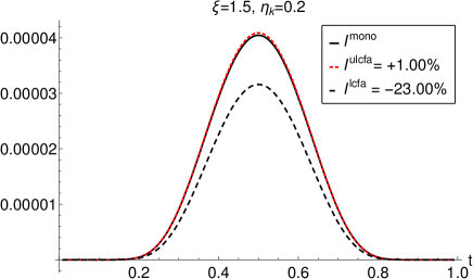
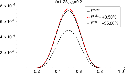
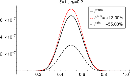
Figure 1: Comparison of the LCFA and ULCFA to the exact analytical result for a circularly-polarised monochromatic background. The percentages in boxes are the relative errors in the integral, calculated by integrating the curve over $t$. The relative error is further investigated in Fig. 2.

Example spectra are compared in Fig. 1. In general, the LCFA and ULCFA both increase in accuracy as $\xi$ is increased from $\xi=1$. However, it can be seen that the ULCFA is substantially more accurate than the LCFA in the region close to $\xi\approx 1$, where the LCFA is not expected to be accurate. In Fig. 2a, it is demonstrated how this accuracy also depends on the energy parameter $\eta_{k}$. If $\xi$ is reduced below $\xi=1$, the ULCFA begins to be less accurate than the LCFA. In Fig. 2b, it is shown that for small energy parameter, the ULCFA develops large errors.

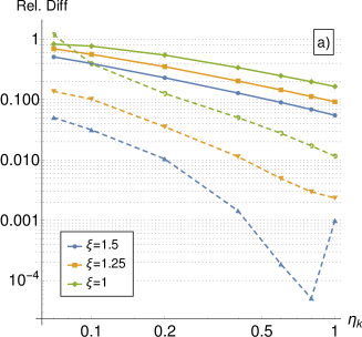
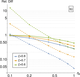
Figure 2: A comparison of the absolute relative error of the LCFA (solid lines) and ULCFA (dashed lines), compared to the analytical monochromatic result of the integrated rate $|\int\,\mathcal{I}\,dt/\int\,\mathcal{I}^{\textsf{mono}}\,dt-1|$.

Here we see the motivation for introducing the intensity filter in the definition of the ULCFA in Eq. (12). If $\xi$ and $\eta$ are small, naïvely using the modified Airy arguments can lead to a poor approximation. However, this is easy to accomodate for, by using an intensity filter, such that when $\xi(\phi)<\xi^{\ast}$, the LCFA is chosen in preference to the ULCFA. To determine $\xi^{\ast}$, one could use the intersection of the ULCFA and LCFA curves in Fig. 2b for whichever seed photon energy was being used. Because we are interested in demonstrating the efficacy of the ULCFA in modelling upcoming high-energy experiments such as LUXE and E320, where $\eta_{k}\sim O(0.1)$, in the following, we simply set $\xi^{\ast}=0.7$ without recourse to optimisation.

II.2 Numerical evaluation of pulse integral

In studies of the accuracy of the LCFA in modelling nonlinear Compton scattering, it was noted Harvey et al. (2015) that since the LCFA only samples “local” parts of the background, it cannot include significant interference effects, which are required to produce a harmonic structure. However, the situation in pair-creaton is different, because the mass gap defines a threshold harmonic, which, for electron beam energies available in upcoming particle-physics experiments (of the order of $10\,\textrm{GeV}$), is already of the order of $n\sim O(10)$. We know that as $n\to\infty$, the Bessel functions in monochromatic rates for nonlinear Compton and pair-creation can be well-approximated by their asymptotic limit Seipt et al. (2017); NIST (2017), which are Airy functions, corresponding to the CCF result. So we could expect that the LCFA and ULCFA can be potentially better approximations for pair-creation than nonlinear Compton scattering, which has no such limitation on the minimum contributing harmonic, other than $n>0$. However, there is an extra source of structure in finite pulsed backgrounds, which originates from the pulse envelope. It was shown Heinzl et al. (2010) that when the laser-averaged lightfront momentum transfer is a multiple of the laser carrier frequency, a finite-pulse harmonic resonance effect causes sub peaks to appear in the spectrum. This clearly cannot be modelled by the LCFA nor by monochromatic rates.

In order to investigate how well the ULCFA performs for finite pulses, we use a finite $\cos^{2}$ pulse with scaled vector potential:

$$a=(0,a^{\perp},0,0);\quad a^{\perp}=m\xi\cos^{2}\left(\frac{\pi\phi}{2\Phi}\right)\,\sin\phi,$$ (21)

$\Phi=2\pi N$, $N\in\mathbb{Z}$ and $|\phi|<\Phi$ (we have specifically chosen a potential that vanishes asymptotically to avoid infra-red effects Dinu et al. (2012)). For circularly-polarised backgrounds, we might expect the ULCFA to be particularly good because $a^{2}$ is a constant and the only $\phi$-dependent term in the Kibble mass is the term linear in $a$. For this reason, we test the ULCFA with the above linearly-polarised pulse. We then compare the phase-integrated spectrum, $\mathcal{S}$, defined e.g. for the ULCFA as:

$$\mathcal{S}^{\scriptsize\textsf{ULCFA}} = \int_{-\infty}^{\infty}d\phi~{}\mathcal{I}^{\tiny\textsf{ULCFA}}(\phi),$$ (22)

where we note that now, $\mathcal{S}$ is a function of:

$$\mathcal{S}=\mathcal{S}(\Phi,t,\xi,\eta),$$

in other words, the instantaneous dependency of $\mathcal{I}$ on $\phi$ has become a “global” dependency of $\mathcal{S}$ on $\Phi$. For the pulse, we numerically evaluate Eq. (I) with the scaled vector potential Eq. (21). To perform the calculation, we use the Bakhvalov-Vasil’eva method Bakhvalov and Vasil’eva (1968), which we briefly detail in Appendix A.

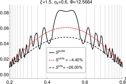
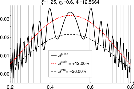
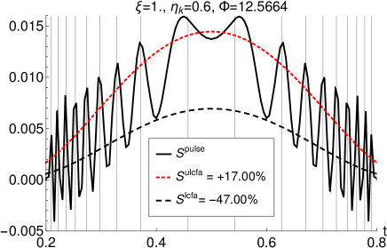
Figure 3: Example plots of spectra in a pulse, showing the interference structure ($\eta_{k}=0.6$ corresponds to a frequency-tripled optical background). The harmonic subpeaks are correctly predicted by taking a cycle-average of the momentum relation Eq. (23) for integer multiples of the fast laser pulse frequency.

Some example spectra are plotted in Fig. 3, where we see that for finite pulses, the ULCFA also performs better than the LCFA. We note the general trend that, for higher intensity there is better agreement between the local approximations and the finite pulse result. We also note that we are able to successfully predict the position of the pulse resonance subpeaks by a simple kinematic analysis. Consider energy-momentum conservation in a quasi-periodic field:

$$k+C\varkappa=P+Q,$$

where $P$ and $Q$ are the quasimomenta of the electron and positron respectively $P=p+\varkappa(\xi^{2}/2\varkappa\cdot p)$ and likewise for $Q$, where $C$ is an initially unknown real number. Squaring both sides of the energy-momentum conservation equation and assuming that, on average, $\mathbf{p}^{\perp}=\mathbf{q}^{\perp}=\boldsymbol{0}$, one acquires an equation to solve for the lightfront momentum fraction $t$:

$$C\eta_{k}=(1+\xi^{2})\left[1+\frac{1-t}{2t}+\frac{t}{2(1-t)}\right].$$ (23)

Now, this is very similar to the case of a circularly-polarised monochromatic background and making the comparison turns out to be useful. The main differences are, that for a finite pulse, $C$ is not an integer, and $\xi^{2}$ is not a constant. Therefore, it can be the case that the harmonic structure in a finite pulse is not well defined. This is clear, because to acquire a perfectly harmonic structure in the monochromatic derivation, one assumes that the background is constant in amplitude (and hence infinite in extent). This enters in the calculational step:

$$\sum_{n,n^{\prime}}F_{n,n^{\prime}}\lim_{L\to\infty}\int_{-L/2}^{L/2}\,d\phi~{}\mbox{e}^{i\phi(n-n^{\prime})}\to 2\pi\sum_{n}F_{n,n},$$

which is an integration over the external-field phase $\phi$, where $n$ and $n^{\prime}$ are integers arising from decomposing the monochromatic background using the Jacobi-Anger relation Berestetskii et al. (1982) and $F_{n,n^{\prime}}$ is the phase-independent probability rate. This turns a double harmonic sum, which includes interference between harmonics, into a purely harmonic expansion. Should either of the assumptions be false, the periodic symmetry of the background would be broken, and we should expect any harmonics to be “smoothed out” by interference. In Eq. (23), we can take the cycle average of $(1+\xi^{2})$ over the “fast” part of the oscillation:

$$1+\xi^{2}(\varphi)\to\frac{1}{N\pi}\int_{-2\pi N}^{2\pi N}1+\xi^{2}(x)~{}dx=4\left(1+\frac{3\,\xi^{2}}{16}\right),$$

and if we take the constant $C$ to be an integer, i.e. the momentum supplied by the laser field to be an integer multiple of the “fast” oscillation momentum, then we find the agreement given by the vertical grey lines in Fig. 3. However, we note that this is simply a useful observation, not a universal rule - when longer or more intense pulses were used, the agreement was not as clear as implied here, but the agreement demonstrates that the numerical routine is behaving in a logical way.

III Conclusion

We presented a uniform locally constant field approximation (LCFA) for nonlinear Breit-Wheeler pair-creation in a plane wave background. We displayed results where, for $\xi\sim O(1)$, our “ULCFA”, was an order of magnitude more accurate than the LCFA in modelling the lightfront spectrum of pairs generated in the cases investigated: i) a circularly-monochromatic background and ii) a finite short pulse. The reason for the better agreement is that the ULCFA includes higher order derivatives of the background and therefore samples a larger region of the field than the standard LCFA. This extension is in the spirit of Ilderton et al. (2019a), but unlike Ilderton et al. (2019a), a uniform approach was taken and all corrections are within the Airy function arguments of the LCFA. This has the advantage that only one filter needs to be applied, namely an intensity filter which ensures that, when the intensity is weak enough, the LCFA is chosen over the ULCFA. For the short pulse spectrum, we demonstrated a kinematic argument that successfully predicted the positions of harmonic resonant subpeaks due to the finite pulse structure.

The motivation for our work stems from upcoming experiments such as LUXE Altarelli et al. (2019) at DESY and E320 The FACET-II SFQED Collaboration (2019) at FACET-II using high-quality accelerator electron beams of the order of $10\,\textrm{GeV}$, which will be collided with laser pulses with a moderate intensity parameter $\xi\sim O(1)$ to study high-intensity QED. We have demonstrated that LCFA methods can be extended to lower intensities than the standard applicability regime $\xi\gg 1$ and showed that the ULCFA can be accurate to within $10\%$ even down to intensities as low as $\xi\approx 1.25$.

Appendix A Numerical Evaluation of Finite Pulses

We wish to evaluate integrals of the following type:

$$\mathcal{I}=\int_{-\theta_{f}}^{\theta_{f}}\,d\theta~{}f(\theta)\,\mathbb{e}^{icg(\theta)},$$ (24)

where $g(\theta)$ is monotonic in $\theta$ and antisymmetric: $g(-\theta)=-g(\theta)$ and $c$ is some positive non-zero constant. We begin by linearising the exponent, with the substitution: $g(\theta)=\gamma y$, where $\gamma=g(\theta_{f})$ to bring the integral in the form:

$$\mathcal{I}=\int_{-1}^{1}\,dy~{}H(y)\,\mathbb{e}^{ic\gamma y};\quad H(y)=\frac{\gamma\,f[g^{-1}(\gamma y)]}{g^{\prime}\left[g^{-1}(\gamma y)\right]}.$$

At this point, we wish to use the method from Bakhvalov and Vasil’eva Bakhvalov and Vasil’eva (1968) which we were directed to from Olver (2008), which utilises the result:

$$\int_{-1}^{1}dx\,P_{k}(x)\,\mathbb{e}^{i\omega x}=i^{k}\left(\frac{2\pi}{\omega}\right)^{1/2}J_{k+\frac{1}{2}}(\omega),$$

for Legendre polynomials of degree $k$, $P_{k}(x)$, and hence decompose $H(y)$ using the standard result Arfken et al. (2012):

$$H(y)=\sum_{k=0}^{k_{\textsf{max}}}\frac{2k+1}{2}P_{k}(y)\int_{-1}^{1}dy\,H(y)\,P_{k}(y),$$

where $k_{\textsf{max}}$ is determined by a convergence criterion in the numerical evaluation.

There is one subtelty with applying this method to QED processes in a pulse such as given in Eq. (I). If one naïvely applies this method, it will fail due to the divergent $1/\theta$ pre-exponent term. However, the “$i\varepsilon$” prescription gives a factor $-\pi/2$ from the $\theta$ integral, which we can rewrite and combine with the naïvely-divergent term in the following way (see also Dinu et al. (2014)).

$$\mathfrak{I} = \int_{-\infty}^{\infty}\,d\theta~{}\frac{1}{\theta}\,\mathbb{e}^{icg(\theta)}-\frac{\pi}{2}$$

$$= \int_{-\infty}^{\infty}\,d\theta~{}\frac{1}{\theta}\,\mathbb{e}^{icg(\theta)}-\int_{0}^{\infty}\,d\left[g(\theta)\right]\,\frac{\sin cg(\theta)}{g(\theta)}$$

$$= \int_{-\infty}^{\infty}\,d\theta~{}\left[\frac{1}{\theta}-\frac{g^{\prime}(\theta)}{g(\theta)}\right]\,\mathbb{e}^{icg(\theta)}$$

$$= \int_{-1}^{1}\,dy~{}\left[\frac{1}{g^{\prime}[g^{-1}(\gamma y)]}\frac{1}{g^{-1}(\gamma y)}-\frac{1}{y}\right]\,\mathbb{e}^{ic\gamma y},$$

(the change in integral limits is made in recognition of the integrand disappearing outside of the pulse). At this point, the Bakhvalov Vasil’eva method can then be applied. Examples of our results using this method, are given in the main body of the paper in Fig. 3

References

- Breit and Wheeler (1934) G. Breit and J. A. Wheeler, Phys. Rep. 46, 1087 (1934).
- Nikishov and Ritus (1964) A. I. Nikishov and V. I. Ritus, Sov. Phys. JETP 19, 529 (1964).
- Narozhnyĭ (1969) N. B. Narozhnyĭ, Sov. Phys. JETP 28, 371 (1969).
- Brezin and Itzykson (1970) E. Brezin and C. Itzykson, Phys. Rev. D 2, 1191 (1970).
- Heinzl et al. (2010) T. Heinzl, A. Ilderton, and M. Marklund, Phys. Lett. B 692, 250 (2010).
- Nousch et al. (2012) T. Nousch, D. Seipt, B. Kämpfer, and A. I. Titov, Phys. Lett. B 715, 246 (2012).
- Titov et al. (2012) A. I. Titov, H. Takabe, B. Kampfer, and A. Hosaka, Phys. Rev. Lett. 108, 240406 (2012), eprint 1205.3880.
- Titov et al. (2019) A. I. Titov, A. Otto, and B. Kampfer (2019), eprint 1907.00643.
- Di Piazza (2016) A. Di Piazza, Phys. Rev. Lett. 117, 213201 (2016).
- Di Piazza et al. (2012) A. Di Piazza et al., Rev. Mod. Phys. 84, 1177 (2012).
- King and Heinzl (2016) B. King and T. Heinzl, High Power Laser Science and Engineering 4, e5 (2016), eprint hep-ph/1510.08456.
- Narozhny and Fedotov (2015) N. B. Narozhny and A. M. Fedotov, Contemporary Physics 56, 249 (2015).
- Hu (2019) H. Hu (2019), eprint 1907.03786.
- Harvey et al. (2015) C. N. Harvey, A. Ilderton, and B. King, Phys. Rev. A 91, 013822 (2015).
- Di Piazza et al. (2018) A. Di Piazza, M. Tamburini, S. Meuren, and C. H. Keitel, Phys. Rev. A 98, 012134 (2018), URL https://link.aps.org/doi/10.1103/PhysRevA.98.012134.
- Ilderton et al. (2019a) A. Ilderton, B. King, and D. Seipt, Phys. Rev. A 99, 042121 (2019a), URL https://link.aps.org/doi/10.1103/PhysRevA.99.042121.
- Ritus (1985) V. I. Ritus, J. Russ. Laser Res. 6, 497 (1985).
- Katkov and Baier (1994) V. M. Katkov and V. N. Baier, Electromagnetic Processes at High Energies in Oriented Single Crystals (World Scientific Publishing, 1994).
- Blackburn et al. (2019) T. G. Blackburn, D. Seipt, S. S. Bulanov, and M. Marklund (2019), eprint 1904.07745.
- Di Piazza et al. (2019) A. Di Piazza, M. Tamburini, S. Meuren, and C. H. Keitel, Phys. Rev. A 99, 022125 (2019), URL https://link.aps.org/doi/10.1103/PhysRevA.99.022125.
- Aleksandrov et al. (2019) I. A. Aleksandrov, G. Plunien, and V. M. Shabaev, Phys. Rev. D 99, 016020 (2019), URL https://link.aps.org/doi/10.1103/PhysRevD.99.016020.
- Ilderton et al. (2019b) A. Ilderton, B. King, and A. J. Macleod (2019b), eprint 1907.12835.
- A. Ilderton, B. King and S. Tang (2019) A. Ilderton, B. King and S. Tang, One-photon pair-annihilation in pulsed plane-wave backgrounds, (to appear) (2019).
- Nerush et al. (2011) E. N. Nerush et al., Phys. Rev. Lett. 106, 035001 (2011).
- Elkina et al. (2011) N. V. Elkina et al., Phys. Rev. ST Accel. Beams 14, 054401 (2011).
- Ridgers et al. (2012) C. P. Ridgers, C. S. Brady, R. Duclous, J. G. Kirk, K. Bennett, T. D. Arber, A. P. L. Robinson, and A. R. Bell, Phys. Rev. Lett. 108, 165006 (2012), URL https://link.aps.org/doi/10.1103/PhysRevLett.108.165006.
- King et al. (2013) B. King, N. Elkina, and H. Ruhl, Phys. Rev. A 87, 042117 (2013).
- Bulanov et al. (2013) S. S. Bulanov, C. B. Schroeder, E. Esarey, and W. P. Leemans, Phys. Rev. A 87, 062110 (2013), URL https://link.aps.org/doi/10.1103/PhysRevA.87.062110.
- Ridgers et al. (2014) C. Ridgers, J. Kirk, R. Duclous, T. Blackburn, C. Brady, K. Bennett, T. Arber, and A. Bell, Journal of Computational Physics 260, 273 (2014), ISSN 0021-9991, URL http://www.sciencedirect.com/science/article/pii/S0021999113008061.
- Blackburn (2015) T. G. Blackburn, Plasma Physics and Controlled Fusion 57, 075012 (2015), URL https://doi.org/10.1088%2F0741-3335%2F57%2F7%2F075012.
- Gelfer et al. (2015) E. G. Gelfer, A. A. Mironov, A. M. Fedotov, V. F. Bashmakov, E. N. Nerush, I. Y. Kostyukov, and N. B. Narozhny, Phys. Rev. A 92, 022113 (2015), URL https://link.aps.org/doi/10.1103/PhysRevA.92.022113.
- Jirka et al. (2016) M. Jirka, O. Klimo, S. V. Bulanov, T. Z. Esirkepov, E. Gelfer, S. S. Bulanov, S. Weber, and G. Korn, Phys. Rev. E 93, 023207 (2016), URL https://link.aps.org/doi/10.1103/PhysRevE.93.023207.
- Gonoskov et al. (2017) A. Gonoskov, A. Bashinov, S. Bastrakov, E. Efimenko, A. Ilderton, A. Kim, M. Marklund, I. Meyerov, A. Muraviev, and A. Sergeev, Phys. Rev. X 7, 041003 (2017), URL https://link.aps.org/doi/10.1103/PhysRevX.7.041003.
- Efimenko et al. (2019) E. S. Efimenko, A. V. Bashinov, A. A. Gonoskov, S. I. Bastrakov, A. A. Muraviev, I. B. Meyerov, A. V. Kim, and A. M. Sergeev, Phys. Rev. E 99, 031201 (2019), URL https://link.aps.org/doi/10.1103/PhysRevE.99.031201.
- Sarri et al. (2014) G. Sarri et al., Phys. Rev. Lett. 113, 224801 (2014).
- Sarri et al. (2015) G. Sarri et al., Nature communications 6, 6747 (2015).
- Cole et al. (2018) J. M. Cole, K. T. Behm, E. Gerstmayr, T. G. Blackburn, J. C. Wood, C. D. Baird, M. J. Duff, C. Harvey, A. Ilderton, A. S. Joglekar, et al., Phys. Rev. X 8, 011020 (2018), URL https://link.aps.org/doi/10.1103/PhysRevX.8.011020.
- Poder et al. (2018) K. Poder, M. Tamburini, G. Sarri, A. Di Piazza, S. Kuschel, C. D. Baird, K. Behm, S. Bohlen, J. M. Cole, D. J. Corvan, et al., Phys. Rev. X 8, 031004 (2018), URL https://link.aps.org/doi/10.1103/PhysRevX.8.031004.
- Harding and Lai (2006) A. K. Harding and D. Lai, Rep. Prog. Phys. 69, 2631 (2006).
- Yokoya and Chen (1992) K. Yokoya and P. Chen, in Frontiers of Particle Beams: Intensity Limitations, edited by M. Dienes, M. Month, and S. Turner (Springer Berlin Heidelberg, Berlin, Heidelberg, 1992), pp. 415–445, ISBN 978-3-540-46797-7.
- Miller and Good (1953) S. C. Miller and R. H. Good, Phys. Rev. 91, 174 (1953), URL https://link.aps.org/doi/10.1103/PhysRev.91.174.
- Valleé and Soares (2010) O. Valleé and M. Soares, Airy Functions and Applications to Physics (Imperial College Press, 57 Selton Street, Covent Garden, London WC2H 9HE, 2010).
- Dunne and Unsal (2014) G. V. Dunne and M. Unsal, Phys. Rev. D89, 105009 (2014), eprint 1401.5202.
- Altarelli et al. (2019) M. Altarelli, R. Assmann, F. Burkart, B. Heinemann, T. Heinzl, T. Koffas, A. R. Maier, D. Reis, A. Ringwald, and M. Wing (2019), eprint 1905.00059.
- The FACET-II SFQED Collaboration (2019) The FACET-II SFQED Collaboration, Probing Strong-field QED at FACET-II (SLAC E-320), (to appear) (2019).
- Burke et al. (1997a) D. L. Burke, R. C. Field, G. Horton-Smith, J. E. Spencer, D. Walz, S. C. Berridge, W. M. Bugg, K. Shmakov, A. W. Weidemann, C. Bula, et al., Phys. Rev. Lett. 79, 1626 (1997a), URL https://link.aps.org/doi/10.1103/PhysRevLett.79.1626.
- Burke et al. (1997b) D. L. Burke et al., Phys. Rev. Lett. 79, 1626 (1997b).
- Bamber et al. (1999) C. Bamber et al., Phys. Rev. D 60, 092004 (1999).
- Turcu et al. (2016) I. C. E. Turcu et al., Rom. Rep. Phys. 68, S145 (2016).
- Shen et al. (2018) B. Shen, Z. Bu, J. Xu, T. Xu, L. Ji, R. Li, and Z. Xu, Plasma Phys. Control. Fusion 60, 044002 (2018).
- Seipt and Thomas (2019) D. Seipt and A. G. R. Thomas, Plasma Phys. Control. Fusion 61, 074005 (2019), eprint 1903.11463.
- Note (1) Note1, for example, on P. 551 of the review Ritus (1985), also reported in Hartin et al. (2019).
- Dinu and Torgrimsson (2018) V. Dinu and G. Torgrimsson, Phys. Rev. D97, 036021 (2018), eprint 1711.04344.
- Dinu and Torgrimsson (2019) V. Dinu and G. Torgrimsson, Phys. Rev. D99, 096018 (2019), eprint 1811.00451.
- Note (2) Note2, recent work has shown that the order in which such limits are taken is crucial, and that they are not, in general, commutative Ilderton (2019).
- Olver (1997) F. W. J. Olver, Asymptotics and Special Functions (AKP Classics, A K Peters Ltd., 63 South Avenue, Natick, MA 01760, 1997).
- Seipt et al. (2017) D. Seipt, T. Heinzl, M. Marklund, and S. S. Bulanov, Phys. Rev. Lett. 118, 154803 (2017), URL https://link.aps.org/doi/10.1103/PhysRevLett.118.154803.
- NIST (2017) NIST, Nist digital library of mathematical functions, http://dlmf.nist.gov/ (2017).
- Dinu et al. (2012) V. Dinu, T. Heinzl, and A. Ilderton, Phys. Rev. D 86, 085037 (2012).
- Bakhvalov and Vasil’eva (1968) N. Bakhvalov and L. Vasil’eva, USSR Comput. Math. Math. Phys. 8, 241 (1968).
- Berestetskii et al. (1982) V. B. Berestetskii, E. M. Lifshitz, and L. P. Pitaevskii, Quantum Electrodynamics (second edition) (Butterworth-Heinemann, Oxford, 1982).
- Olver (2008) S. Olver, Ph.D. thesis, University of Cambridge (2008).
- Arfken et al. (2012) G. B. Arfken, H. J. Weber, and F. E. Harris, Mathematical Methods for Physicists (Elsevier, 2012), seventh ed.
- Dinu et al. (2014) V. Dinu, T. Heinzl, A. Ilderton, M. Marklund, and G. Torgrimsson, Phys. Rev. D 89, 125003 (2014), URL http://link.aps.org/doi/10.1103/PhysRevD.89.125003.
- Hartin et al. (2019) A. Hartin, A. Ringwald, and N. Tapia, Phys. Rev. D 99, 036008 (2019), URL https://link.aps.org/doi/10.1103/PhysRevD.99.036008.
- Ilderton (2019) A. Ilderton, Phys. Rev. D 99, 085002 (2019), URL https://link.aps.org/doi/10.1103/PhysRevD.99.085002.