Deep Learning for Segmentation using an Open Large-Scale Dataset in 2D Echocardiography

Abstract

Delineation of the cardiac structures from 2D echocardiographic images is a common clinical task to establish a diagnosis. Over the past decades, the automation of this task has been the subject of intense research. In this paper, we evaluate how far the state-of-the-art encoder-decoder deep convolutional neural network methods can go at assessing 2D echocardiographic images, i.e. segmenting cardiac structures as well as estimating clinical indices, on a dataset especially designed to answer this objective. We therefore introduce the Cardiac Acquisitions for Multi-structure Ultrasound Segmentation (CAMUS) dataset, the largest publicly-available and fully-annotated dataset for the purpose of echocardiographic assessment. The dataset contains two and four-chamber acquisitions from 500 patients with reference measurements from one cardiologist on the full dataset and from three cardiologists on a fold of 50 patients. Results show that encoder-decoder based architectures outperform state-of-the-art non-deep learning methods and faithfully reproduce the expert analysis for the end-diastolic and end-systolic left ventricular volumes, with a mean correlation of 0.95 and an absolute mean error of 9.5 ml. Concerning the ejection fraction of the left ventricle, results are more contrasted with a mean correlation coefficient of 0.80 and an absolute mean error of 5.6%. Although these results are below the inter-observer scores, they remain slightly worse than the intra-observer’s ones. Based on this observation, areas for improvement are defined, which open the door for accurate and fully-automatic analysis of 2D echocardiographic images.

I Introduction

Analysis of 2D echocardiographic images plays a crucial role in clinical routine to measure the cardiac morphology and function and to reach a diagnosis. Such analysis is based on the interpretation of clinical indices which are extracted from low-level image processing such as segmentation and tracking. For instance, the extraction of the ejection fraction (EF) of the left ventricle (LV) requires accurate delineation of the left ventricular endocardium in both end diastole (ED) and end systole (ES). In clinical routine, semi-automatic or manual annotation is still daily work due to the lack of accuracy and reproducibility of fully-automatic cardiac segmentation methods. This leads to time consuming tasks prone to intra- and inter-observer variability [1]. The inherent difficulties for segmenting echocardiographic images are well documented: i) poor contrast between the myocardium and the blood pool; ii) brightness inhomogeneities; iii) variation in the speckle pattern along the myocardium due to the orientation of the cardiac probe with respect to tissue; iv) presence of trabeculae and papillary muscles with intensities similar to the myocardium; v) significant tissue echogenicity variability within the population; vi) shape, intensity and motion variability of the heart structures across patients and pathologies.

The lack of large and publicly-available dataset has prevented a thorough evaluation of the potential of deep learning methods to estimate clinical indices, while these techniques are actively applied with great success for other modalities [2]. Indeed, while the number of medical imaging challenges comparing deep learning methods has exploded this last decade, only one focused on cardiac ultrasound image segmentation [3]. Unfortunately, since the challenge was held in 2014, none of the participant used convolutional neural networks (CNNs) because these methods had not yet gained popularity in medical imaging. The lack of well-annotated echocardiographic datasets can be explained by the difficulty of exporting data from clinical ultrasound equipments and getting a large amount of images carefully annotated by cardiologists due to the very nature of echocardiography as mentioned above. In this context, the purpose of this paper is to provide answers to the following four questions:

1. How well do CNNs perform compared to non-deep learning state-of-the-art techniques ?

2. How many patients are needed to train a CNN to get highly accurate results in 2D echocardiographic image segmentation ?

3. How accurate can the volumes and ejection fraction be estimated from the segmentation of CNNs compared to the inter/intra-expert variability ?

4. What improvement can be brought by sophisticated architectures compared to simpler CNN models for 2D echocardiographic segmentation ?

For that purpose, we present a new public dataset called CAMUS (Cardiac Acquisitions for Multi-structure Ultrasound Segmentation). It contains $2$D echocardiographic sequences with two and four-chamber views of $500$ patients that were acquired with the same equipment in the same medical center. The size of this dataset and its tight connection to every-day clinical issues give the possibility to train deep learning methods to automatically analyze echocardiographic data. In addition, CAMUS includes manual expert annotations for the left ventricle endocardium (LV_Endo), the myocardium (epicardium contour more specifically, named LV_Epi) and the left atrium (LA).

II Previous work

Previous cardiac ultrasound datasets

To date, only one echocardiographic dataset has been broadly validated. This dataset was released in conjunction with the Challenge on Endocardial Three-dimensional Ultrasound Segmentation (CETUS) which took place during the MICCAI 2014 conference. The CETUS dataset is composed of $45$ $3$D echocardiographic sequences ($15$ for training, $30$ for testing) equally distributed among three different subgroups: healthy subjects, patients with previous myocardial infarction examined at least 3 months after the event and patients with dilated cardiomyopathy. The data is provided with two reference meshes of the LV_Endo per patient (one at ED and one at ES), each reference corresponding to the mean shape computed from the annotations of three different experienced cardiologists. Five fully-automatic (deformable models, Hough random forest, Kalman filter, active appearance model) and four semi-automatic methods (graph-cut method, structured random forest, multi-atlas and level-set approaches) were evaluated through this challenge. No challenger implemented a deep neural network. The outcome of the challenge revealed that the overall best scores were obtained by the B-spline explicit active surface, a fully-automatic method proposed by Barbosa et al. [4]. This method was later on improved by Pedrosa et al. [5] thanks to the integration of a shape prior derived from a conventional principal component analysis scheme. By doing so, the authors obtained the following scores for the segmentation of the $3$D LV_Endo: i) average Dice values of $0.909$ (ED) and $0.875$ (ES); ii) average Hausdorff distances of $6.3$ mm (ED) and $6.9$ mm (ES) and iii) average mean absolute distances of $1.8$ mm (ED) and $2.0$ mm (ES).

Non-deep learning methods

Several surveys of echocardiographic segmentation methods have been proposed, both in 2D [6, 7] and 3D [3, 8]. Most of the reported methods focused on the segmentation of the LV_Endo border. Among those reviews, only the one by Bernard et al. published in 2016 benchmarked different techniques on the same dataset, leading to a fair comparison [3]. In this study, the authors listed the results obtained by nine different techniques. The reported methods can be divided in two main categories: those with a weak prior and those with a strong prior. The first group involves weak assumptions such as spatial, intensity, motion or anatomical information. It includes image-based techniques (multi-scale quadrature filter) [9], a motion-based method (Kalman filter) [10], deformable models (BEAS, level-set) [4, 9] and a graph-based approach (graph-cut) [11]. The second group uses approaches with strong priors including a shape-prior (Hough forest) [12], an active appearance model [13], an atlas-based method [14] and a machine learning algorithm (random forest) [12, 15, 16], each requiring a manually-annotated training set.

Deep learning methods

Deep-learning methods have been successfully applied to the segmentation of the LV_Endo in echocardiography. In 2012, Carneiro et al. developed a two-stage deep learning method for the segmentation of the LV_Endo for 2D echocardiographic images restricted to four-chamber view acquisitions [7]. Based on a maximum a posteriori framework, the authors formulated the LV segmentation problem according to two successive steps: i) the automatic selection of several regions in the tested image where the LV_Endo is fully present; ii) the automatic extraction of the LV_Endo contour from the previously selected regions. These two steps involved a deep belief network. Their method was trained on 400 images from $12$ different patient sequences with various pathologies and tested on 50 images from $2$ healthy subject sequences. They obtained an average Hausdorff distance of $\sim\!\!18$ mm and an average mean absolute distance of $\sim\!\!8$ mm for the LV_Endo.

In 2017, Smistad et al. [17] showed that the U-Net CNN method [18] could be trained to successfully segment the left ventricle in 2D ultrasound images. However, due to lack of training data, the network was trained with the output of a state-of-the-art deformable model segmentation method [10]. On a manually segmented test set, the results showed that the network and the deformable model obtained the same accuracy with a Dice score of 0.87.

Recently, Oktay et al. [19] used CNNs to segment the 3D LV_Endo structure using an approach named anatomically constrained neural network (ACNN). The core of their neural network is based on an architecture similar to the 3D U-Net [20], whose segmentation output is constrained to fit a non-linear compact representation of the underlying anatomy derived from an auto-encoder network. The performance of their method was assessed on the CETUS dataset. They obtained the following scores for the segmentation of the 3D LV_Endo structure: i) average Dice values of $0.912$ (ED) and $0.873$ (ES); ii) average Hausdorff distances of $7.0$ mm (ED) and $7.7$ mm (ES) and iii) average mean absolute distances of $1.9$ mm (ED) and $2.1$ mm (ES) [19]. Interestingly, these results are quite close to those obtained by Pedrosa et al. [5]. Additionally, the use of only $15$ patients during the training phase illustrates the strong potential of deep learning techniques to analyze echocardiographic images.

III CAMUS dataset

III-A Dataset

As described in the previous section, only one echocardiographic dataset, composed of 45 3D sequences, has been broadly validated by the community. This dataset is not appropriate to study the behavior of deep learning approaches in the particular case of 2D sequences. In this context, we introduce the largest publicly-available and fully annotated dataset for the purpose of 2D echocardiographic assessment.

III-A1 Patient selection

The proposed dataset consists of clinical exams from 500 patients, acquired at the University Hospital of St Etienne (France) and included in this study within the regulation set by the local ethical committee of the hospital. The acquisitions were optimized to perform LV_EF measurements. In order to enforce clinical realism, neither prerequisite nor data selection have been performed. Consequently, i) some cases were difficult to trace; ii) the dataset involves a wide variability of acquisition settings; iii) for some patients, parts of the wall were not visible in the images; iv) for some cases, the probe orientation recommendation to acquire a rigorous four-chambers view was simply impossible to follow and a five-chambers view was acquired instead. This produced a highly heterogeneous dataset, both in terms of image quality and pathological cases, which is typical of daily clinical practice data. Table LABEL:tab:dataset provides the main information which characterizes the collected dataset. From this table, one can see that half of the dataset population has a LV_EF lower than $45$%, thus being considered at pathological risk (beyond the uncertainty of the measurement). Also, $19$% of the images have a poor quality (based on the opinion of one expert O_1a), indicating that for this subgroup the localization of the LV_Endo  and LV_Epi  as well as the estimation of clinical indices are not considered clinically accurate and workable. In classical analysis, poor quality images are usually removed from the dataset because of their clinical uselessness. Therefore, those data were not involved in this project during the computation of the different metrics but were used to study their influence as part of the training and validation sets for deep learning techniques.

TABLE I: The main characteristics of the CAMUS echocardiographic dataset collected from $500$ patients

Dataset	Image Quality			LVEF
	(in percentage)			(in percentage)
	Good	Medium	Poor	$\leq 45$%	$\geq 55$%	else
Full	35	46	19	49	19	32
fold 1	34	48	18	48	20	32
fold 2	34	46	20	50	18	32
fold 3	34	46	20	48	20	32
fold 4	34	46	20	50	20	30
fold 5	34	46	20	48	20	32
fold 6	36	46	18	50	20	30
fold 7	36	46	18	50	20	30
fold 8	36	46	18	50	18	32
fold 9	36	46	18	48	20	32
fold 10	36	46	18	50	18	32

The dataset was divided into 10 folds to perform standard cross-validation for the machine learning methods. Each fold contains $50$ patients with the same distributions in terms of image quality and LV_EF as the full dataset (see table LABEL:tab:dataset). For each of the 10 test sets, the remaining $450$ patients ($9$ folds) were used during the training/validation phases of the machine learning techniques. In particular, $8$ folds ($400$ patients) were used for training and $1$ ($50$ patients) for validation, i.e. parameters optimization. The full dataset is available for download at https://camus.creatis.insa-lyon.fr/challenge/,.

III-A2 Acquisition protocol

The full dataset was acquired from GE Vivid E95 ultrasound scanners (GE Vingmed Ultrasound, Horten Norway), with a GE M5S probe (GE Healthcare, US). No additional protocol than the one used in clinical routine was put in place. For each patient, $2$D apical four-chamber and two-chamber view sequences were exported from EchoPAC analysis software (GE Vingmed Ultrasound, Horten, Norway). These standard cardiac views were chosen for this study to enable the estimation of LV_EF values based on the Simpson’s biplane method of discs [21]. Each exported sequence corresponds to a set of B-mode images expressed in polar coordinates. The same interpolation procedure was used to express all sequences in Cartesian coordinates with a unique grid resolution, i.e. $\lambda/2=0.3$ mm along the x-axis (axis parallel to the probe) and $\lambda/4=0.15$ mm along the z-axis (axis perpendicular to the probe), where $\lambda$ corresponds to the wavelength of the ultrasound probe. At least one full cardiac cycle was acquired for each patient in each view, allowing manual annotation of cardiac structures at ED and ES.

III-B Reference segmentation and contouring protocol

Establishing a well-defined ground-truth segmentation was of utmost importance for this work. The main difficulty when delineating 2D echocardiographic images comes from poor contrast in some regions along with the presence of well-known artifacts (e.g. reverberation, clutter, acoustic shadowing). One direct consequence is that embedded fully-automatic ultrasound cardiac segmentation softwares do not perform well. During the clinical exam, the clinicians delineate the different contours using semi-automatic tools under time constraints. In this context, the use of manual annotations extracted from clinical exams is not optimal to design a reference dataset for machine learning where the coherence and accuracy in the manual contouring play an important role during the learning phase. To illustrate this point, it is interesting to note that the only existing shared echocardiographic dataset with reference annotations was realized off-line for the purpose of the CETUS MICCAI challenge in 2014. In particular, it required more than 10 months for 3 different cardiologists to manually contour the 3D endocardium surfaces of $45$ patients including consensus revisions [3]. This illustrates the extreme difficulty in designing such a high-quality dataset.

III-B1 Cardiologists involvement

Three cardiologists (O₁, O₂ and O₃) participated in the annotation of the dataset. Considerable effort was spent to define a consistent manual segmentation protocol. This protocol was designed with the help of O₁ and was then strictly followed O₂ and O₃. In particular, we asked O₁ to perform the manual annotation and to determine ED and ES of the full dataset, while the two others contoured the test set of fold $5$ ($50$ patients). O₁ also annotated twice fold $5$ seven months apart (we call those annotations O_1a and O_1b). This fold was therefore used to measure both the inter- and intra-observer variability.

III-B2 Contouring protocol

According to the recommendation of the American Society of Echocardiography and the European Association of Cardiovascular Imaging [22], ED is preferably defined as the first frame after mitral valve closure or the frame in the cardiac cycle in which the respective LV dimension or volume measurement is the largest. ES is best defined as the frame after aortic valve closure (e.g. using an apical long axis view image) or the frame in which the cardiac dimension or volume is the smallest. In this work, ED and ES were selected as the frames where the LV dimension was at its largest or smallest, which is not the most accurate way, especially in the presence of abnormalities. This simpler approach was used due to the lack of reliable ECG. Thus the clinical indices, ED/ES volume and EF, reported in this work have to be interpreted with this in mind. While only the extraction of the LV_Endo contour is necessary to estimate LV_EF values, we also asked the cardiologists to manually outline the LV_Epi and the LA for all patients. This was done to study the influence of contextualization (segmentation of several structures at once) on the performance of the LV_Endo segmentation using deep learning techniques. The following protocol was set up.

• LV_Endo: Convention was used for the LV wall, mitral valve plane, trabeculations, papillary muscles and apex [22]. Basic points were to i) include trabeculae and papillary muscles in the LV cavity; ii) keep tissue consistency between ED and ES instants; iii) terminate the contours in the mitral valve plane on the ventricular side of the bright ridge, at the points where the valve leaflets are hinging; iv) partially exclude left ventricular outflow tract from the cavity by drawing from septal mitral valve hinge point to the septal wall to create a smooth shape.

• LV_Epi: There is no recommendation for delineating the epicardium. We thus outlined the epicardium as the interface between the pericardium and the myocardium for the anterior, anterolateral and inferior segments and the frontier between the right ventricle cavity and the septum for the inferoseptal segments.

• LA: There are recommendations for LA segmentation to assess the full LA area from dedicated LA recordings. However, since we have used acquisitions focusing on the LV, part of the dataset does not cover the full LA surface and is thus not suited to perform such measurement. Having this in mind, we used the following contouring protocol: i) start the LA contour from the extremities of the LV_Endo contour, at the points where the valve leaflets are hinging; ii) have the contour pass by the LA inner border.

Fig. 1 illustrates our manual contouring protocol for a good, a medium, and a poor-quality image.

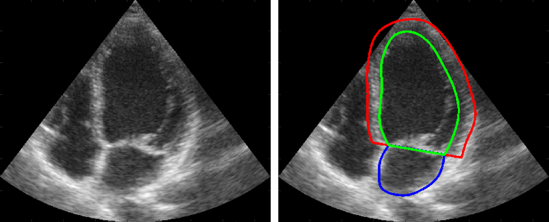
(a) Good image quality

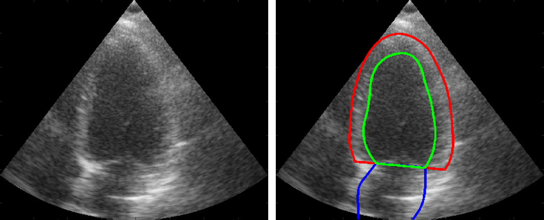
(b) Medium image quality

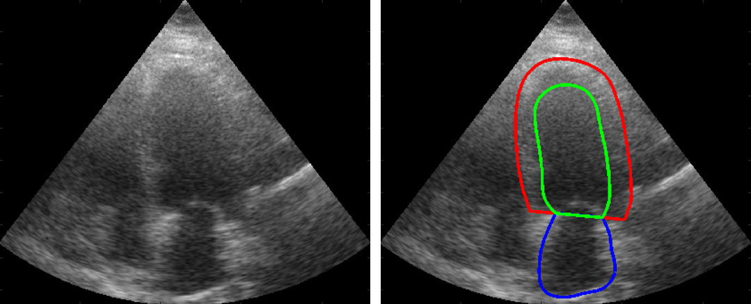
(c) Poor image quality

Figure 1: Typical images extracted from the proposed dataset. Endocardium and epicardium of the left ventricle and left atrium wall are shown respectively in green, red and blue. [Left] input images; [Right] corresponding manual annotations.

IV Evaluated methods

IV-A CNN techniques based on an encoder-decoder architecture

The goal of this study is to assess how far CNNs can go at segmenting 2D echocardiographic images. As such, we chose to focus on the well-known encoder-decoder networks (EDNs) which have been the cornerstone of a wide variety of CNNs that were successfully applied in medical imaging [23]. EDNs are based on a two-stage convolutional network architecture well suited for segmentation. The first part, known as the encoder, consists of a series of convolutions and downsampling operations. These operations extract features from the images while spatially compressing them, thus enabling extraction of high-level features. The second part is the decoder, which uses features from the encoder and applies a set of convolutions and upsampling operations to gradually transform feature maps into a final segmentation.

Among the existing EDNs, one of the most popular architectures used in medical imaging corresponds the U-Net model proposed by Ronneberger et al. in 2015 [18]. This network integrates skip connections between the encoder and decoder parts with the goal of helping in retrieving details that were potentially lost during the downsampling while also stabilizing gradients. The original U-Net follows a specific scheme of convolutions, where each downsampling and upsampling step is proceeded by two 3x3 convolutional layers, while the number of features is doubled per downsampling and reduced in half per upsampling. U-Net has been successfully applied to a wide range of medical applications [23], but for each application, the network design has usually been adapted and optimized to get the best segmentation performance on each application. The main U-Net design choices can be classified in three categories: i) layer choices: convolutional layer size, activation functions, normalization layers, down- and upsampling strategies (e.g. max pooling, striding, deconvolution and repeat); ii) the optimization process (gradient descent strategy, weight initialization, loss function, batch size, regularization constraints, stopping criteria, deep supervision, dropout); iii) data handling (pre-processing, augmentation, sampling). Since the seminal paper in 2015, several studies based on the EDN structure have been carried out with the goal of outperforming the U-Net. Among those methods, two types of approaches have been proposed: those based on U-Net architecture but with extensions such as shape regularization [19] and those with more sophisticated architectures [24, 25]. In this context, we decided to benchmark the following EDNs for the purpose of segmenting 2D echocardiographic images:

IV-A1 U-Net

Taking into account the wide range of possible U-Net designs, we decided to compare the performance of two independent implementations, i.e. U-Net 1 optimized for speed, and U-Net 2 optimized for accuracy. This leads to two different architectures (which both differ from the original one proposed by Ronneberger et al.) with their own hyperparameters settings, as shown in table LABEL:tab:unets. The “number of feature maps” column given in table LABEL:tab:unets corresponds to the number of convolutions in the convolution layers. For each U-Net implementation, we successively indicate the values for the first, the bottom (where the spatial information is the most compressed), and the last convolution layers. U-Net 1 & 2 enable to investigate the impact of hyperparameters choices on the quality of the results. The total number of parameters for U-Net 1 and 2 are 2.0M and 17.5M, respectively.

IV-A2 ACNN

Starting from a given segmentation architecture, this method integrates an auxiliary loss to constrain the segmentation output to fit a non-linear compact representation of the underlying anatomy derived from an auto-encoder network  [19]. For comparison purposes, we used the U-Net 1 architecture described in table LABEL:tab:unets as the segmentation module in our ACNN implementation. Moreover, the following choices were made to obtain the best results on our dataset: i) a code of $32$ coefficients was set for the auto-encoder network (which allows an average reconstruction accuracy of $97\%$); ii) the hyperparameter balancing the segmentation and shape regularization losses was set so that the two losses had close initialization values. The ACNN models in our study have 2.2M parameters.

IV-A3 SHG

Stacked Hourglasses (SHG) method integrates three successive encoder-decoder networks (usually three times the same architecture) where the first two are used as residual blocks [24]. Each output of the encoder-decoder networks is associated with an intermediate segmentation loss. This strategy is called deep supervision. The output of the third network is used as the final segmentation result. For comparison purposes, we also used the U-Net 1 architecture as the key encoder-decoder network in our SHG implementation. The number of parameters of the SHG method is 4.5M (not 6M in order to keep the same batch size as U-Net 1).

IV-A4 U-Net++

This method is also based on deep supervision technique but with the integration of additional convolution layers in the form of dense skip connections [25]. Starting from the official online version of the code, we adapted the corresponding architecture to obtain the best results on our dataset. The following changes were made: i) dropout was removed; ii) averaging of the last feature maps of the intermediate outputs was removed; iii) the original design of layers was adapted according to the choices we made to optimized U-Net 1 architecture; iv) the batch size was set to 20. The U-Net++ method comprises 1.1M parameters. The original version had 9M parameters but we adapted it, in particular the number of feature maps, so to get the best possible results on the CAMUS dataset.

Please note that the same data pre- and post-processing strategies (i.e. connected component analysis keeping the largest region and removing holes) were applied for each of the evaluated method. For completeness’ sake, implementation details of the two U-Net architectures as well as additional tests on ACNN and U-Net++ can be found in the supplementary materials. Supplementary materials are available in the supplementary files /multimedia tab.

TABLE II: Main characteristics of U-Net 1 and U-Net 2. More details are provided in the supplementary materials /multimedia tab.

Architectures	Number of	Lowest	Upsampling	Normalization	Batch	Learning	Loss	# Trainable
	feature maps	Resolution	Scheme	Scheme	Size	Rate	Function	Parameters
U-Net 1	$32\downarrow 128\uparrow 16$	$8*8$	$2*2$ repeats	None	32	1e-3	Multi-class Dice	2M
U-Net 2	$32\downarrow 512\uparrow 32$	$16*16$	Deconvolutions	BatchNorm	10	1e-4	Cross-entropy	18M
							+ weight decay

IV-B Non-deep learning state-of-the-art techniques

To compare the performance of the EDN methods described above, we implemented the following non-deep learning state-of-the-art methods which obtained among the best results during the CETUS challenge [3] and which were recently improved [5] and applied in 2D [26].

IV-B1 SRF

Structured Random Forests (SRF) refer to an ensemble learning method for classification or regression. It operates at training time by building a set of decision trees that assign a label patch to each input image patch, computed as the mean prediction of the individual trees [27]. During the training phase, each tree individually learns a set of split functions from a random subset of the training dataset and input features. Those functions are intended to group patches sharing close image intensities and segmentation patterns. During the testing phase, the image to segment is fragmented into different overlapping patches. Each image patch goes through the splitting functions of each tree so that the mean label patch computed from the reached leaves forms its segmentation. Detailed description of the SRF algorithm implemented in this project can be found in [26]. Compared to our previous study, data was not split between ES and ED nor between 4 chambers and 2 chambers views but processed in one indistinctive pool of images. Since CAMUS has a larger number of patients than the dataset used in [26], we trained $12$ individual trees for each subset of $100$ patients.

IV-B2 BEASM

The key concept of the B-Spline Explicit Active Surface Model (BEASM) framework is to consider the boundary of a deformable interface as an explicit function, where one of the coordinates of the points within the surface is given explicitly as a function $\psi$ of the remaining coordinates. In this framework, $\psi$ is defined as a linear combination of B-spline basis functions whose controlled knots are located on a regular rectangular grid defined on the chosen coordinate system (polar space in our case). Based on a standard variational approach, the evolution of the deformable surface is then governed by the minimization of an energy function according to the B-spline coefficients [28]. This framework has been successfully applied in [29] for the coupled segmentation of the LV_Endo and LV_Epi structures in echocardiography and further extended by the integration of a shape prior directly into the B-spline space in  [5], named as BEASM in the rest of the paper. Because BEASM amounts to a deformable-based model, the initialization of the contour plays a crucial role on the quality of the results. We thus decided to implement two different strategies: i) one named BEASM-fully where the evolving contour is automatically initialized from a method inspired by the work proposed in [30]; ii) another named BEASM-semi where the evolving contour is initialized from three points (two at the base and one at the apex of the LV_Endo structure) extracted from the reference contours. By doing so, we gave the possibility to quantify the influence of the initialization procedure for BEASM on an heterogeneous ultrasound dataset.

V Results

As stated in Section III-A, the 19% of poor quality images were not used to compute the different metrics provided in this part. Moreover, to avoid the use of different models according to the acquisition settings, we trained only one model for each machine learning method on both apical four-chamber and two-chamber views regardless of the time instant in the cardiac sequence. For a detailed analysis of the results, a set of complementary information are provided in the supplementary materials (i.e. figures of segmentation results for all the methods, Bland-Altman plots, limitations examples). Supplementary materials are available in the supplementary files /multimedia tab.

V-A Evaluation metrics

V-A1 Geometrical metrics

To measure the accuracy of the segmentation output (LV_Endo, LV_Epi or LA) of a given method, the Dice metric, the mean absolute distance ($d_{m}$) and the 2D Hausdorff distance ($d_{H}$) were used. The Dice similarity index is defined as $D=2\left(\left|S_{user}\cap S_{ref}\right|\right)/\left(\left|S_{user}\right|+\left|S_{ref}\right|\right)$ and is a measure of overlap between the segmented surface $S_{user}$ extracted from a method and the corresponding reference surface $S_{ref}$. The Dice index gives a value between 0 (no overlap) and 1 (full overlap). $d_{m}$ corresponds to the average distance between $S_{user}$ and $S_{ref}$ while $d_{H}$ measures the local maximum distance between the two surfaces.

V-A2 Clinical metrics

We gauge the methods’ performance with $3$ clinical indices: i) the ED volume (LV_EDV in $ml$); ii) the ES volume (LV_ESV in $ml$); iii) the ejection fraction (LV_EF as a percentage) for which we computed four metrics: the correlation ($corr$), the bias and the standard deviation ($std$) values (computed from conventional definitions) and the mean absolute error ($mae$). The combination of the bias and standard deviation also provides useful information on the corresponding limit of agreement values.

V-B Empirical results

TABLE III: Segmentation accuracy (LV_Endo and LV_Epi) of the $8$ evaluated methods on the ten test folds of table LABEL:tab:dataset restricted to patients having good & medium image quality ($406$ patients in total). All the metrics were computed using the annotations of expert O_1a. All the scores obtained with the U-Net 2, which is the overall best performing method, were statistically different with a p-value $<0.05$ (computed with a Wilcoxon signed-rank test) compared to all the tested methods, except U-Net 1 and SHG for the d_H metric.

Methods *	ED						ES
	$\boldsymbol{LV\textsubscript{Endo}}$			$\boldsymbol{LV\textsubscript{Epi}}$			$\boldsymbol{LV\textsubscript{Endo}}$			$\boldsymbol{LV\textsubscript{Epi}}$
	D	dm	dH	D	dm	dH	D	dm	dH	D	dm	dH
	val.	mm	mm	val.	mm	mm	val.	mm	mm	val.	mm	mm
O1a vs O2	0.919	2.2	6.0	0.913	3.5	8.0	0.873	2.7	6.6	0.890	3.9	8.6
(inter-obs)	$\pm$0.033	$\pm$0.9	$\pm$2.0	$\pm$0.037	$\pm$1.7	$\pm$2.9	$\pm$0.060	$\pm$1.2	$\pm$2.4	$\pm$0.047	$\pm$1.8	$\pm$3.3
O1a vs O3	0.886	3.3	8.2	0.943	2.3	6.5	0.823	4.0	8.8	0.931	2.4	6.4
(inter-obs)	$\pm$0.050	$\pm$1.5	$\pm$2.5	$\pm$0.018	$\pm$0.8	$\pm$2.6	$\pm$0.091	$\pm$2.0	$\pm$3.5	$\pm$0.025	$\pm$1.0	$\pm$2.4
O2 vs O3	0.921	2.3	6.3	0.922	3.0	7.4	0.888	2.6	6.9	0.885	3.9	8.4
(inter-obs)	$\pm$0.037	$\pm$1.2	$\pm$2.5	$\pm$0.036	$\pm$1.5	$\pm$3.0	$\pm$0.058	$\pm$1.3	$\pm$2.9	$\pm$0.054	$\pm$1.9	$\pm$2.8
O1a vs O1b	0.945	1.4	4.6	0.957	1.7	5.0	0.930	1.3	4.5	0.951	1.7	5.0
(intra-obs)	$\pm$0.019	$\pm$0.5	$\pm$1.8	$\pm$0.019	$\pm$0.9	$\pm$2.3	$\pm$0.031	$\pm$0.5	$\pm$1.8	$\pm$0.021	$\pm$0.8	$\pm$2.1
SRF	0.895	2.8	11.2	0.914	3.2	13.0	0.848	3.6	11.6	0.901	3.5	13.0
	$\pm$0.074	$\pm$3.6	$\pm$10.2	$\pm$0.057	$\pm$2.0	$\pm$9.1	$\pm$0.137	$\pm$7.8	$\pm$13.6	$\pm$0.078	$\pm$4.7	$\pm$11.1
BEASM-fully	0.879	3.3	9.2	0.895	3.9	10.6	0.826	3.8	9.9	0.880	4.2	11.2
	$\pm$0.065	$\pm$1.8	$\pm$4.9	$\pm$0.051	$\pm$2.1	$\pm$5.1	$\pm$0.092	$\pm$2.1	$\pm$5.1	$\pm$0.054	$\pm$2.0	$\pm$5.1
BEASM-semi	0.920	2.2	6.0	0.917	3.2	8.2	0.861	3.1	7.7	0.900	3.5	9.2
	$\pm$0.039	$\pm$1.2	$\pm$2.4	$\pm$0.038	$\pm$1.6	$\pm$3.0	$\pm$0.070	$\pm$1.6	$\pm$3.2	$\pm$0.042	$\pm$1.7	$\pm$3.4
U-Net 1	0.934	1.7	5.5	0.951	1.9	5.9	0.905	1.8	5.7	0.943	2.0	6.1
	$\pm$0.042	$\pm$1.0	$\pm$2.9	$\pm$0.024	$\pm$0.9	$\pm$3.4	$\pm$0.063	$\pm$1.3	$\pm$3.7	$\pm$0.035	$\pm$1.2	$\pm$4.1
U-Net 2	0.939	1.6	5.3	0.954	1.7	6.0	0.916	1.6	5.5	0.945	1.9	6.1
	$\pm$0.043	$\pm$1.3	$\pm$3.6	$\pm$0.023	$\pm$0.9	$\pm$3.4	$\pm$0.061	$\pm$1.6	$\pm$3.8	$\pm$0.039	$\pm$1.2	$\pm$4.6
ACNN	0.932	1.7	5.8	0.950	1.9	6.4	0.903	1.9	6.0	0.942	2.0	6.3
	$\pm 0.034$	$\pm 0.9$	$\pm 3.1$	$\pm 0.026$	$\pm 1.1$	$\pm 4.1$	$\pm 0.059$	$\pm 1.1$	$\pm 3.9$	$\pm 0.034$	$\pm 1.2$	$\pm 4.2$
SHG	0.934	1.7	5.6	0.951	1.9	5.7	0.906	1.8	5.8	0.944	2.0	6.0
	$\pm 0.034$	$\pm 0.9$	$\pm 2.8$	$\pm 0.023$	$\pm 1.0$	$\pm 3.3$	$\pm 0.057$	$\pm 1.1$	$\pm 3.8$	$\pm 0.034$	$\pm 1.2$	$\pm 4.3$
U-Net ++	0.927	1.8	6.5	0.945	2.1	7.2	0.904	1.8	6.3	0.939	2.1	7.1
	$\pm 0.046$	$\pm 1.1$	$\pm 3.9$	$\pm 0.026$	$\pm 1.0$	$\pm 4.5$	$\pm 0.060$	$\pm 1.0$	$\pm 4.2$	$\pm 0.034$	$\pm 1.1$	$\pm 5.1$
* LVEndo: Endocardial contour of the left ventricle; LVEpi: Epicardial contour of the left ventricle; ED: End diastole
ES: End systole; D: Dice index; dm: mean absolute distance; dH: Hausdorff distance; mae: mean absolute error
The values in bold refer to the best performance for each measure.
The inter and intra-observer measurements were computed from fold 5 restricted to patients having good & medium
image quality (40 patients)

V-B1 Geometrical scores

Table III shows the segmentation testing accuracy computed from patients having good and medium image quality ($406$ patients) for the 8 algorithms described in section IV. Mean and standard deviation values for each metric were obtained from cross-validating on the $10$ folds of the dataset. The values in bold correspond to the best scores for each metric. From these results, one can see that the EDN implementations get the overall best segmentation scores on all metrics, for both ED and ES. Interestingly, while the EDN methods are fully-automatic, they still get better segmentation results than the semi-automatic BEASM algorithm.

The two U-Nets achieve equivalent results for all the metrics compared to the ones obtained by the more sophisticated encoder-decoder architectures. This hints to the idea that a plateau has been reached, which classical tuning, shape regularization techniques and more sophisticated architectures have difficulties to overcome. This also suggests that a U-Net implementation, which requires less parameters than SHG and U-Net++ methods and less training time than ACNN, offers the best compromise between the network size and performance for the particular task of 2D echocardiographic image segmentation.

To assess the influence of the layer design in the performance between U-Net 1 and 2, statistical significance of their respective results was analyzed by performing the Wilcoxon signed-rank test for each metric. Results showed that U-Net 1 and 2 produced scores that are statistically different (p-value $<0.05$) for most metrics at ED and ES, apart for the LV_Epi Hausdorff distance. However, this must be nuanced by the fact that i) the U-Net geometrical scores are very close (mean d_m and d_H difference of $0.1$ mm and $0.1$ mm, respectively), producing distributions with high degree of overlap as shown in the supplementary materials /multimedia tab; ii) the U-Net geometrical results lie between the inter-observer and intra-observer scores for all metrics, proving the robustness of this method in obtaining accurate segmentation results. As a complement to the above, we investigated in the supplementary materials /multimedia tab the influence of each of the U-Net hyperparameters presented in table LABEL:tab:unets. Results highlight the importance of the choice of the normalization scheme.

As for the fully automatic non-deep learning state-of-the-art methods, BEASM-auto obtained on average better Hausdorff distances (mean $d_{H}$ of $9.9$ mm at ED and $10.5$ mm at ES) while the SRF got better Dice and $d_{m}$ scores (mean $d_{m}$ of $3.0$ mm at ED and $3.5$ mm at ES). However, the large standard deviation values for the SRF illustrate the difficulties of this method in obtaining consistent segmentations over the entire dataset. As for the BEASM-semi, one can see that the manual initialization has a strong impact on the quality of the results, with a mean improvement of $0.8$ mm and $2.4$ mm for the $d_{m}$ and $d_{H}$ metrics, respectively. Moreover, it is well known that the left ventricle shape is more difficult to segment at ES, leading to slightly worse performance for classical algorithms on this time instant. This property is also confirmed in our study since all the evaluated methods produced better results at ED on every metric.

As complement, we provided in the supplementary materials /multimedia tab the geometrical scores obtained on the poor quality images ($94$ patients) for the 8 evaluated algorithms. For this part of the dataset, the EDNs also obtained the best segmentation results on all metrics. Interestingly, while EDN scores on poor quality images are slightly worse than those computed on good and medium quality, they remain very competitive compared to the scores given in table III (mean LV_Endo d_m and d_H of $2.2$ mm and $7.0$ mm and mean LV_Epi d_m and d_H of $2.3$ mm and $7.6$ mm).

TABLE IV: Clinical metrics of the $8$ evaluated methods on the ten test folds of table LABEL:tab:dataset restricted to patients having good & medium image quality ($406$ patients in total). All the metrics were computed using the annotations of expert O_1a. Volumes and ejection fraction obtained with U-Net 2 were statistically different with p-values $<0.05$ (computed with the Wilcoxon signed-rank test) compared to all the tested methods, except SHG for the LV_ESVindice.

Methods *	LVEDV			LVESV			LVEF
	corr	bias$\pm\sigma$	mae	corr	bias$\pm\sigma$	mae	corr	bias$\pm\sigma$	mae
	val.	ml	ml	val.	ml	ml	val.	%	%
O1a vs O2 (inter-obs)	0.940	18.7$\pm$12.9	18.7	0.956	18.9$\pm$9.3	18.9	0.801	-9.1$\pm$8.1	10.0
O1a vs O3 (inter-obs)	0.895	39.0$\pm$18.8	39.0	0.860	35.9$\pm$17.1	35.9	0.646	-12.6$\pm$10.0	13.4
O2 vs O3 (inter-obs)	0.926	-20.3$\pm$15.6	21.0	0.916	-17.0$\pm$13.5	17.7	0.569	3.5$\pm$11.0	8.5
O1a vs O1b (intra-obs)	0.978	-2.8$\pm$7.1	6.2	0.981	-0.1$\pm$5.8	4.5	0.896	-2.3$\pm$5.7	0.9
SRF	0.755	-0.2$\pm$25.7	17.4	0.827	9.3$\pm$18.0	14.8	0.465	-11.5$\pm$15.4	12.8
BEASM-fully	0.704	13.4$\pm$30.6	22.9	0.713	18.0$\pm$25.8	22.5	0.731	-9.8$\pm$8.3	10.7
BEASM-semi	0.886	14.6$\pm$19.2	17.8	0.880	18.3$\pm$16.9	19.5	0.790	-9.4$\pm$7.2	10.0
U-Net 1	0.947	-8.3$\pm$12.6	10.9	0.955	-4.9$\pm$9.9	8.2	0.791	-0.5$\pm$7.7	5.6
U-Net 2	0.954	-6.9 $\pm$11.8	9.8	0.964	-3.7$\pm$ 9.0	6.8	0.823	-1.0$\pm$7.1	5.3
ACNN	0.945	-6.7$\pm$ 12.9	10.8	0.947	-4.0$\pm$ 10.8	8.3	0.799	-0.8$\pm$7.5	5.7
SHG	0.943	6.4$\pm$12.8	10.5	0.938	-3.2$\pm$11.3	8.2	0.770	-1.4$\pm$7.8	5.7
U-Net ++	0.946	-11.4$\pm$ 12.9	13.2	0.952	-5.7$\pm$ 10.7	8.6	0.789	-1.8$\pm$ 7.7	5.6
* corr: Pearson correlation coefficient; mae: mean absolute error.
The values in bold refer to the best performance for each measure.
The inter and intra-observer measurements were computed from fold 5 restricted to patients having good & medium
image quality (40 patients.)

V-B2 Clinical scores

Table IV contains the clinical metrics for the $8$ methods. Those indices were computed with the Simpson’s rule [21] from the segmentation results of each algorithm. The values in bold represent the best scores for the corresponding index. As for segmentation, the EDNs obtained the best clinical scores on all the tested metrics (bias was not taken into account since the lowest bias value in itself does not necessarily mean the best performing method). Regarding the estimation of the LV_EDV and LV_ESV, the EDNs obtained high correlation scores (all above $0.94$) and reasonably small biases (at most $11.4$ ml), standard deviations (less than $12.9$ ml) and mean absolute errors (at most $13.2$ ml). Results are more contrasted for the estimation of the LV_EF. For this metric, the EDNs got lower correlation scores (at most $0.82$) but smaller biases (less than $1.8$ %), standard deviations (at most $7.8$ %) and mean absolute errors (less than $5.7$ %). It is worth pointing out that average EDN scores are all below the inter-observer scores. This proves the clinical interest of such approaches but also reveals the needs for improvement as discussed in Section V-D. Here again, even if the U-Net methods involved simpler architecture, they obtained similar results compared to the more sophisticated EDNs. Finally, using the Wilcoxon signed-rank test, U-Net 1 and U-Net 2 produced LV_EDV, LV_ESV and LV_EF results whose difference is statistically significant (p-values $<0.05$), although their measurements are very close.

V-C U-Net behavior

From the results given in table III and IV, it appears that the U-Net method has the most effective architecture among the tested EDN models in terms of trade-off between the number of parameters and the achieved performance for the particular task of 2D echocardiographic image analysis. To better analyze the behavior of this model, we set up several additional experiments whose results are provided in Fig. 2 and Fig. 3. For all these experiments, even if the acquisitions were optimized to perform LV_EF measurements (meaning that part of the LA may or may not be fully visible depending on the acquisitions), we also investigated the capacity of U-Net to segment the LA in addition to the $LV_{endo}$ and $LV_{epi}$. Moreover, since the two tested U-Nets produced overall close geometrical and clinical scores, we only used in this part the U-Net 1 model since it requires considerably less parameters to learn. Finally, all the given metrics were computed from both four and two-chamber views and at ED and ES time instants to facilitate the interpretation of the results.

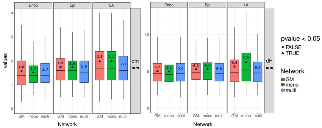
Figure 2: Tukey box plots computed from the geometrical results of the U-Net 1 architecture for three different schemes (GM for learning to simultaneously segment all three structures from good & medium image quality, mono for learning to segment one structure from all image quality, multi for learning to simultaneously segment all three structures from all image quality). Blue numbers correspond to mean values computed from each set of measurements. All p-values are based on the Wilcoxon signed-rank test computed with the multi strategy as reference.

V-C1 Mono versus multi-structures approaches

We assessed the influence of learning strategies on the quality of the segmentation of the LV_Endo, LV_Epi and LA. In particular, we trained 4 models with the same U-Net 1 architecture but with different training sets including all image quality, i.e. one network trained on predicting only the LV_Endo, one the LV_Epi, one the LA, and one all structures. Results on the full dataset are plotted in green and blue in Fig. 2 and are referred to as mono and multi.

From the derived box plots, one can see that, unrelated to the structure, the mono and multi-structures approaches produced very close results even if the corresponding differences are statistically different. These results show that, with the proposed implementations, learning the segmentation of one structure (e.g. LV_Endo) in the context of the others (e.g. LV_Epi & LA) does not improve significantly the results compared to learning the segmentation of the structure alone. This hints at designing dedicated architectures and/or loss functions to better exploit the contextual information provided in the segmentation masks. Furthermore, even if the segmentation of the LA structure is challenging compared to  LV_Epi  and LV_Endo  due to acquisition conditions, the U-Net 1 manages to get close results both in terms of mean absolute distance (mean $d_{m}$ equals to $1.7$, $1.9$ and $2.1$ mm for the LV_Endo, LV_Epi and LA respectively) and average Hausdorff distance (mean $d_{H}$ equals to $5.6$, $6.0$ and $6.4$ mm for the LV_Endo, LV_Epi and LA respectively).

V-C2 The effect of poor quality images

We investigated in Fig. 2 the influence of involving images of poor quality during the training phase. Based on a multi-structures scheme, we trained two U-Net 1 models with the same architecture, one using the full training dataset not caring for image quality (plotted in blue and referred as multi in Fig. 2) and one using the training dataset restricted to patients having good and medium image quality (plotted in red and referred as GM in Fig. 2). From the obtained box plots, one can observe that the two different strategies produced very close results even if the corresponding differences are mostly statistically significant (apart for the $d_{m}$ metric for the LV_Endo and LV_Epi). These results suggest that the $19$% ($94$ patients) of poor quality images i) do not bring additional information (supporting that the remaining deep learning issues are weakly linked to image quality); ii) do not decrease performance compared to a model trained on the $406$ patients with good and medium image quality. This result suggests that poor image quality, in itself, does not complicate the segmentation task as much as could be expected and that encoder-decoder based techniques are able to cope with the variability in image quality found in echocardiography.

V-C3 Influence of the size of the training dataset

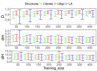
Figure 3: Evolution of the segmentation scores (computed from fold 5 and from both ED and ES time instants) derived from the U-Net 1 architecture according to an incremental increase of the number of patients involved in the training dataset. Dots correspond to mean values while bars correspond to standard deviations.

We studied in Fig. 3 the influence of the size of the training dataset on the quality of the segmentation of the LV_Endo, LV_Epi and LA structures. To this aim, we set up $8$ different experiments, where the same fold $5$ and $6$ were respectively used as test and validation sets. As for the training set, starting from 50 patients, we added for each new experiment 50 additional patients until 400 patients was reached for the last trial. In each experiment, the same U-Net 1 architecture was used and optimized in the same way to derive the best performing parameters from the validation set. Moreover, the number of training epochs was proportionally lowered to ensure that each network went through the same number of iterations.

From this figure, one can first observe an overall improvement of all metrics for the three cardiac structures with the increasing number of patients in the training set. Interestingly, while the improvement between $50$ to $200$ patients is quite pronounced (e.g. a decrease of $d_{H}$ for the LV_Endo from $7.2$ mm to $5.8$ mm), one can observe a change in the evolution of the performance of the U-Net 1 method from $250$ patients. Indeed, for this particular value, results worsen a bit, which may be explained by the bias brought by the validation and test data as we are not doing cross-validation in this experiment. Moreover, from this value, the $d_{m}$ scores seem to stabilize around $1.8$ mm for the LV_Endo, $1.9$ mm for the LV_Epi and $1.8$ mm for the LA structure. The same conclusions can be made for the Dice metric, with a convergence value around $0.920$ for the LV_Endo, $0.947$ for the LV_Epi and $0.909$ for the LA structure. As for the $d_{H}$ metric, while some improvement can still be observed from $250$ to $400$ patients for the LV_Epi and LA structures ($1.1$ mm and $1.0$ mm for the LV_Epi and the LA, respectively), it is not obvious to draw the same conclusion for the LV_Endo structure since the decrease of its corresponding value is less pronounced ($0.2$ mm). In the light of these results, the U-Net 1 implementation performs better that the state-of-the-art non-deep learning methods after training with only $50$ patients. Moreover, this method needs at least $250$ patients during the training phase to reach highly competitive results, which can be slightly improved with a larger training set.

V-C4 Influence of the expert annotations

We investigated in Fig. 4 the influence of the expert annotations during the training phase. To this aim, we trained three models on fold 5 from the same U-Net 1 architecture based each time on the manual contouring from a different annotator. The validation fold was kept the same for each experiment to avoid any bias error. The models were then evaluated on the remaining 400 patients annotated by cardiologist O_1a.

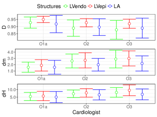
Figure 4: Geometric scores of the three cardiologist-specific models on 400 patients (1600 images)

From this figure, one can observe that the best scores for the three structures are obtained for the model trained on the annotations of cardiologist $O_{1a}$, who performed the manual contouring on the test and validation sets. This observation is consistent with the inter-variability results provided in tables III and IV. It confirms that cardiologists have consistent differences in their way of contouring images and that an EDN has the capacity to learn a specific way of segmenting.

V-C5 Runtime performance

The two U-Nets were implemented in Python with the same version of the TensorFlow and Keras libraries and an Nvidia Tesla M60 GPUs (8 Go RAM). Because of the larger number of trainable parameters involved in the U-Net 2 solution (see table LABEL:tab:unets), the running time of the two networks is different. For the training phase, the time required to train on $400$ patients is $24\pm 5$ min and $73\pm~{}1$ min for the U-Net 1 and U-Net 2, respectively. At test time, the segmentation of a single image takes $0.09\pm~{}0.03$ s and $0.14\pm~{}0.06$ s for the U-Net 1 and U-Net 2, respectively.

V-D Discussion

V-D1 Statistical differences between U-Net 1 and 2 results

From Tables III and IV it has been observed that although U-Net 1 and U-Net 2 have very similar performances, their results were judged most of the time as being statistically different by the Wilcoxon Signed Rank Test (p-value $<0.05$). This can be explained by the fact that when the number of samples is quite high, any slight but consistent deviation between the two distributions will make the difference statistically significant. In our study, since we worked on a large scale dataset, most of the statistical tests were performed on a large amount of samples (for instance Tables III and IV involve more than 800 paired observations for each statistical test), encouraging situations where the differences between results produced by two methods are recognized as statistically significant (even if the evaluated distributions are very close).

V-D2 Inter and intra-observer variability

To further assess the quality of the EDN segmentation results, we added in table III the inter and intra-observer variability measurements computed from fold $5$ (restricted to $40$ patients with good and medium image quality). Concerning the inter-observer variability, the corresponding Dice scores vary between $0.82$ and $0.93$, the $d_{m}$ between $2.2$ mm and $4.0$ mm and the $d_{H}$ between $6.0$ mm and $8.8$ mm. The LV_Epi is the most difficult structure to annotate while both LV_Endo and LV_Epi are harder to contour at ES than at ED. One should also note the large $d_{m}$ value of $4.0$ mm between observer 1a and 3 for the LV_Endo structure at ES. This illustrates i) the difficulty in getting coherent manual annotations between experts from daily clinical practice data; ii) the difficulty for the experts to use unfamiliar software for the analysis; iii) the needs to provide interactively the volumetric results to the experts for instant comparison (this was not done during the manual annotations); iv) the difficulty in contouring some data acquired with non-standard views. Concerning the intra-observer variability, one can observe that the results obtained on all the segmentation scores are better than the inter-observer ones, with a mean difference of $1.5$ mm for the $d_{m}$ metric and $2.6$ mm for the Hausdorff distance. This illustrates the high consistency of manual contouring from experienced cardiologists, even on challenging data. Those results also provide important information on the limits to reach in order to consider that a machine learning algorithm faithfully reproduces the expertise of one cardiologist.

In table IV, we also reported the inter and intra-observer variability measurements computed from fold $5$ (restricted to $40$ patients with good and medium image quality) for the LV_EDV, LV_ESV and LV_EF metrics. From these results, one can observe that the experts reached good agreements for the estimation of the LV_EDV and LV_ESV with mean correlation scores of $0.92$ and $0.91$, respectively. However, the LV_EF results are worse with a mean correlation value of $0.67$. This reveals the extreme difficulty in getting fully consistent manual annotations from ED to ES and between clinicians. It also illustrates the need for semi- or fully-automatic solutions to get higher temporal coherency, as illustrated by the higher LV_EF scores obtained by the semi-automatic BEASM method ($0.79$) and the EDN approaches ($0.79$ on average). Concerning the intra-observer variability, results are much more consistent with mean correlation scores of $0.98$, $0.98$ and $0.90$ of the LV_EDV, LV_ESV and LV_EF metrics, respectively.

V-D3 U-Net versus more sophisticated encoder-decoder architectures

Tables III and IV underlines that U-Net results are very close to those obtained by more sophisticated architectures. This is surprising as one might expect that more complex deep learning designs would improve results, at least marginally. As for ACNN, similar scores may be explained by the simple shapes encountered in 2D echocardiography. Indeed, the reference contours drawn by the experts involve truncated ellipse-like shapes whose information seems to be easily learned by the different EDNs. As a result, the anatomical constraint of the ACNN does not bring any additional value during the segmentation process, leading to similar or even slightly lower performance due to the regularization effect (which can lead to simpler shapes than expected). Further results which support this hypothesis are provided in the supplementary materials /multimedia tab. Concerning SHG and U-Net++, the similar scores may be explained by the results in Fig. 3. From this figure, we observed that U-Net reaches a plateau in terms of its performances when training on more than 250 patients. This suggests that the capacity of a U-Net is sufficient to generalize well on CAMUS dataset. Thus more complex architectures like SHG and U-Net++ did not bring any improvement in our case.

V-D4 Effect of the stochasticity during the training phase

The training of all models in this work is stochastic, thus training a network will not converge to the exact same model each time. To estimate its effect on performance, we provide in table III of the supplementary materials /multimedia tab the results produced by U-Net 1 and U-Net 2 for two different trainings, showing that at worst the d_m and d_H respectively varied of 0.1 and 0.2 mm. The scores obtained with the two U-Net 2 models were consistently better than the ones produced by the U-Net 1 models. This indicates that the effect of the stochastic nature of the training process is limited in our case.

V-D5 Accuracy of EDNs at delineating the LV_Endo , LV_Epi and LA structures

Segmentation results given in table III show that the five EDN implementations clearly outperform the state-of-the-art fully and semi-automatic non-deep-learning methods. In particular, while also learning from annotated data, SRF does not perform as consistently as the EDNs. Concerning the deformable model-based BEASM, even if it integrates the annotated information through a shape prior, this method produces overall significantly less accurate segmentation results. It thus appears from this study that a well-designed EDN can reach impressive segmentation scores in echocardiography. In addition, results given in Section V-C show that U-Net provides the same performances whether low quality data is included or not, and whether the model learns to segment all structures simultaneously or separately (involving three models instead of a single one). U-Net 1 obtained very close results compared to U-Net 2, but with 9 times less parameters. The number of parameters directly influences runtime performance, training time, storage and memory consumption. Since ultrasound is a real-time imaging modality, it would be a huge advantage if a single compact EDN could accurately segment multiple cardiac structures. In this regard, this study indicates that U-Net 1 would be the best candidate to embed into clinical equipment.

Interestingly, the EDN results are better than the inter-observer scores, on all structures and metrics. Although further investigations shall be made to validate this assertion, the obtained results tend to show that, when properly trained, deep learning techniques are able to reproduce manual annotations with high fidelity. The results presented in this pilot study should thus stimulate the community to set up public multi-centric and multi-vendor datasets in echocardiography with annotations from cardiologists having passed high level consensus criteria. It is also interesting to note that EDN results are slightly worse than the intra-observer scores, on all structures and metrics (apart for the $d_{m}$ metric for the LV_Epi at ED). This reveals that even if EDNs produce remarkable results, there still exists room for improvement to faithfully reproduce the manual annotations of one expert, taking into account its variability due to the ultrasound image quality.

In complement, we counted the number of cases for which the EDNs produced results outside the inter-observer variability, i.e. a $d_{m}$ value higher than $3.5$ mm and $4.0$ at ED and ES, respectively and a $d_{H}$ value higher than $8.2$ mm and $8.8$ at ED and ES, respectively. From this experiment, we found that 18% of the segmentations produced by both U-Nets, ACNN or SHG can be seen as outliers. This value goes up to 30 % for U-Net++. For comparison purpose, the outliers rate from two series of annotations on fold 5 produced by the same expert O_1a is equal to 13%. Even if the overall performances of the EDNs are remarkable, this confirms the interest of still improving deep learning solution to produce highly reliable segmentation results on daily clinical practice data.

V-D6 Accuracy of EDNs at estimating clinical indices

Clinical scores provided in table IV show that EDNs produce results below the inter-observer scores for all the metrics. It thus appears that the evaluated EDNs are serious candidates to automatically produce trustworthy estimations of the LV_EDV and LV_ESV indices, on par with medical expertise. Concerning the LV_EF, even if the results are better than the inter-observer scores, a correlation value of $0.82$ (for the best performing method) appears too low in comparison with the intra-observer value of $0.90$ to consider the automatic estimate of this index as sufficiently robust to be dependable in clinical practice. The lower LV_EF scores compared to LV_EDV and LV_ESV measures can be partially explained by the lack of temporal coherency in the tested EDN implementations. Indeed, for each patient, the ED and ES frames are viewed as two independent images, potentially generating less efficient estimation of the corresponding LV_EF measures. Numerous deep learning strategies that integrate temporal coherence such as the recurrent neural networks (the Long Short Term Memory - LSTM - model being one of the famous network of this family) has been described. The integration of such concepts into the U-Net formalism seems to be a solution of interest in order to make the LV_EF estimation more accurate.

VI Conclusions

In this paper, we introduced the largest publicly-available and fully-annotated dataset for 2D echocardiographic assessment (to our knowledge). A dedicated Girder on-line platform has been setup for new result submissions at https://camus.creatis.insa-lyon.fr/challenge/, where the CAMUS dataset, containing 2D apical four-chamber and two-chamber view sequences acquired from 500 patients, is also available for download. Thanks to this dataset, the following new insights were underlined:

• Encoder-decoder networks produced highly accurate segmentation results in 2D echocardiography;

• Among the different tested architectures, U-Net appeared to be most effective in terms of trade-off between the number of parameters and the achieved performance;

• The reasons for the lack of improvement of the more sophisticated networks (ACNN, SHG and U-Net++) compared to U-Net was addressed with additional testings provided in the supplementary materials /multimedia tab;

• U-Net reached a plateau in terms of its performances when training on more than 250 patients but still continued to improve, implying that though 250 patients was enough to generalize well on CAMUS, it has the potential to integrate additional variability;

• U-Net showed impressive robustness to variability, especially to image quality. Considering the wide range of image quality involved in echocardiography, this result is another positive element to consider encoder-decoder-based techniques as a solution of choice to solve the problem of 2D echocardiographic image segmentation;

• U-Net learned to reproduce a specific way of contouring;

• The segmentation and clinical results (left ventricle volumes at ED and ES) of the encoder-decoder networks were all below the inter-observer scores;

• The segmentation and clinical results of the encoder-decoder networks were close to but slightly worse than the intra-observer scores. This reveals that even if encoder-decoder networks produced remarkable results, there is still room for improvement to faithfully reproduce the manual annotation of a given expert.

VII Further details on U-Net 1 and U-Net 2

VII-A Detailed architectures

The two U-Net implementations are summarized in tables I and II. As can be seen, U-Net 1 shows a more compact architecture, with the addition of one downsampling level. In the U-Net 2 design, the number of filters per convolutional layers increases and decreases linearly from an initial kernel size of 48, which makes for a wider net. As can be infered from the small gap in performance between the two architectures, U-Net 1 appears as a more efficient architecture when considering a robustness / capacity trade-off. Please note that the kernel size value corresponds to the number of feature maps (dimensionality of the output of the layer).

TABLE I
U-NET 1 ARCHITECTURE
Level	Layer	Kernel / Pool size	Activation	Connection
D1	Conv	32 (3,3)	ReLU
	Conv	32 (3,3)	ReLU	*
	MaxPooling	(2*2)
D2	Conv	32 (3,3)	ReLU
	Conv	32 (3,3)	ReLU	**
	MaxPooling	(2*2)
D3	Conv	64 (3,3)	ReLU
	Conv	64 (3,3)	ReLU	***
	MaxPooling	(2*2)
D4	Conv	128 (3,3)	ReLU
	Conv	128 (3,3)	ReLU	****
	MaxPooling	(2*2)
D5	Conv	128 (3,3)	ReLU
	Conv	128 (3,3)	ReLU	*****
	MaxPooling	(2*2)
D6	Conv	128 (3,3)	ReLU
	Conv	128 (3,3)	ReLU
U1	UpSampling	(2,2)
	Conv	128 (3,3)	ReLU	*****
	Conv	128 (3,3)	ReLU
U2	UpSampling	(2,2)
	Conv	128 (3,3)	ReLU	****
	Conv	128 (3,3)	ReLU
U3	UpSampling	(2,2)
	Conv	64 (3,3)	ReLU	***
	Conv	64 (3,3)	ReLU
U4	UpSampling	(2,2)
	Conv	32 (3,3)	ReLU	**
	Conv	32 (3,3)	ReLU
U5	UpSampling	(2,2)
	Conv	16 (3,3)	ReLU	*
	Conv	16 (3,3)	ReLU
Seg	Conv	4 (1,1)	Softmax

TABLE II
U-NET 2 ARCHITECTURE
Level	Layer	Kernel / Pool size	Activation	Connection
D1	Conv	48 (3,3)
	BatchNorm		ReLU
	Conv	48 (3,3)
	BatchNorm		ReLU	*
	MaxPooling	(2*2)
D2	Conv	96 (3,3)
	BatchNorm		ReLU
	Conv	96 (3,3)
	BatchNorm		ReLU	**
	MaxPooling	(2*2)
D3	Conv	192 (3,3)
	BatchNorm		ReLU
	Conv	192 (3,3)
	BatchNorm		ReLU	***
	MaxPooling	(2*2)
D4	Conv	384 (3,3)
	BatchNorm		ReLU
	Conv	384 (3,3)
	BatchNorm		ReLU	****
	MaxPooling	(2*2)
D5	Conv	768 (3,3)
	BatchNorm		ReLU
	Conv	768 (3,3)
	BatchNorm		ReLU
U1	ConvTranspose	384 (2,2) - s(2,2)
	BatchNorm		ReLU
	Conv	384 (3,3)		****
	BatchNorm		ReLU
	Conv	384 (3,3)
	BatchNorm		ReLU
U2	ConvTranspose	192 (2,2) - s(2,2)
	BatchNorm		ReLU
	Conv	192 (3,3)		***
	BatchNorm		ReLU
	Conv	192 (3,3)
	BatchNorm		ReLU
U3	ConvTranspose	96 (2,2) - s(2,2)
	BatchNorm		ReLU
	Conv	96 (3,3)		**
	BatchNorm		ReLU
	Conv	96 (3,3)
	BatchNorm		ReLU
U4	ConvTranspose	48 (2,2) - s(2,2)
	BatchNorm		ReLU
	Conv	48 (3,3)		*
	BatchNorm		ReLU
	Conv	48 (3,3)
	BatchNorm		ReLU
Seg	Conv	4 (1,1)	Softmax
s: height and width strides

VII-B Data formatting

For a fair comparison between U-Net implementations, the same data pre- and post-processing were applied. In particular i) images were resized to $256$x$256$ pixels before performing density normalization; ii) no data augmentation strategy was involved; iii) padding was applied before the 3*3 convolutions; iv) initialization of weights were sampled from Glorot uniform distribution; v) $2$*$2$ max-pooling was used as downsampling; vi) ReLu activations were used; vii) segmentation was obtained from a final softmax layer; viii) principal simply connected objects selection was performed to remove small false positive detections. The Adam method was used for stochastic optimization. When learning on the full dataset, the number of epochs was set to 30 and the model that performed best on the validation set was saved.

VII-C From U-Net 1 to U-Net 2

In table LABEL:tab:fromunet1to2, we evaluate how the segmentation accuracy (LV_Endo and LV_Epi) obtained by U-Net 1 on the ten test sets restricted to patients having good or medium image quality ($406$ patients) on ED and ES images is affected when a single hyperparameter differing between U-Net 1 and U-Net 2 is changed. We also retrained a U-Net 1 to see how initialization can impact the results.

As mentioned in the paper, batchNormalization is the only modification that brings an improvement on the LV that is consistently superior to what may be brought by initialization. The loss, the batch size and the upsampling scheme didn’t bring consistent differences. A lower learning rate was slightly detrimental, as the number of epochs is kept the same. Surprisingly, adding more filters doesn’t appear to be meaningfully beneficial, and neither does learning upsampling parameters. Though only the original number of filters was changed here, it suggests that U-Net 1 already has a sufficient number of parameters and that supplementary filters learn redundant information.

TABLE III: Segmentation accuracy (LV_Endo and LV_Epi) from U-Net 1 to U-Net 2.                                                                                                                                   Bold values indicate a superior value to U-Net 1.

Methods *
	$\boldsymbol{LV\textsubscript{Endo}}$			$\boldsymbol{LV\textsubscript{Epi}}$
	D	dm	dH	D	dm	dH
	val.	mm	mm	val.	mm	mm
U-Net 1	0.920	1.7	5.6	0.947	1.9	6.0
	$\pm$0.056	$\pm$1.2	$\pm$3.3	$\pm$0.030	$\pm$1.1	$\pm$3.8
U-Net 1 bis	0.921	1.8	5.5	0.949	1.9	6.0
	$\pm 0.052$	$\pm 1.5$	$\pm 3.1$	$\pm 0.028$	$\pm 1.0$	$\pm 3.5$
U-Net 1 Kernel 48	0.923	1.9	5.5	0.948	1.9	6.0
	$\pm 0.047$	$\pm 1.0$	$\pm 3.2$	$\pm 0.026$	$\pm 1.2$	$\pm 3.8$
U-Net 1 Cross-Entropy loss	0.916	1.9	5.7	0.948	1.9	6.0
	$\pm 0.047$	$\pm 1.3$	$\pm 3.5$	$\pm 0.030$	$\pm 1.0$	$\pm 3.5$
U-Net 1 Conv2DTranspose	0.921	1.7	5.6	0.948	1.9	6.1
	$\pm$0.052	$\pm$1.3	$\pm$3.7	$\pm$0.027	$\pm$1.0	$\pm$4.5
U-Net 1 BatchSize 10	0.923	1.7	5.6	0.949	1.8	6.4
	$\pm$0.055	$\pm$1.0	$\pm$4.3	$\pm$0.031	$\pm$1.1	$\pm$5.2
U-Net 1 LR(1e-4)	0.913	1.9	6.1	0.943	2.1	6.7
	$\pm$0.055	$\pm$1.1	$\pm$3.9	$\pm$0.034	$\pm$1.2	$\pm$4.4
U-Net 1 BatchNorm	0.926	1.6	5.3	0.948	1.9	6.0
	$\pm$0.053	$\pm$1.4	$\pm$3.5	$\pm$0.030	$\pm$1.0	$\pm$3.5
U-Net 2	0.928	1.6	5.4	0.950	1.8	6.1
	$\pm$0.054	$\pm$1.5	$\pm$3.7	$\pm$0.032	$\pm$1.0	$\pm$4.1
U-Net 2 bis	0.930	1.5	5.4	0.951	1.8	5.9
	$\pm$0.049	$\pm$0.9	$\pm$3.4	$\pm$0.024	$\pm$0.9	$\pm$3.3

VII-D Comparison of densities for geometrical metrics

In addition to the p-values obtained from Wilcoxon Signed-Rank tests, we provide visuals of the overlapping distributions of U-Net 1 and U-Net 2 for $d_{m}$ and $d_{H}$ evaluated on the endocardium and the epicardium. As can be seen, both distributions have chi-square aspects, with the production of a few outliers in spite of very good mean performances and overall good robustness.

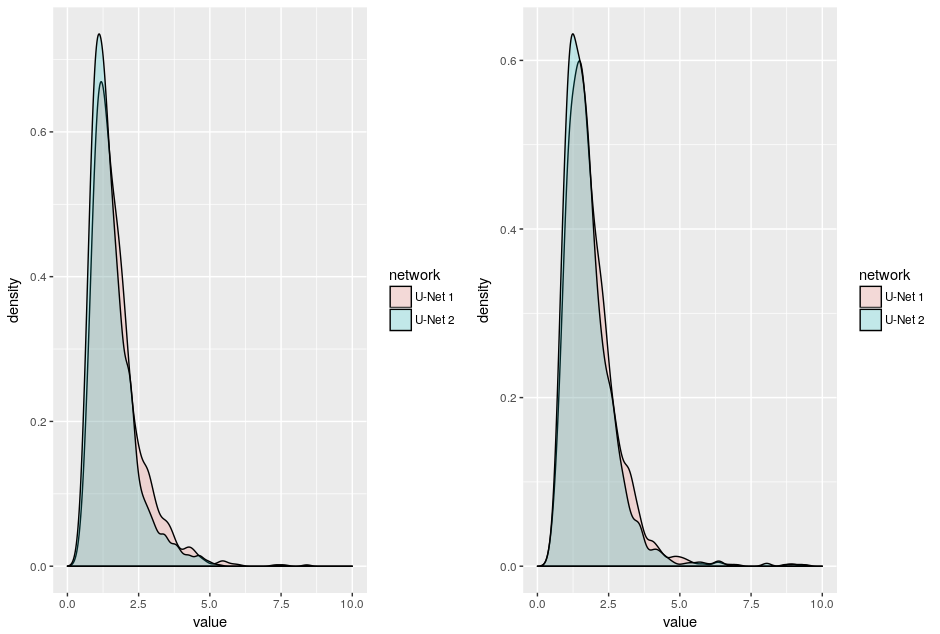
(a) $d_{m}$ endo / epi

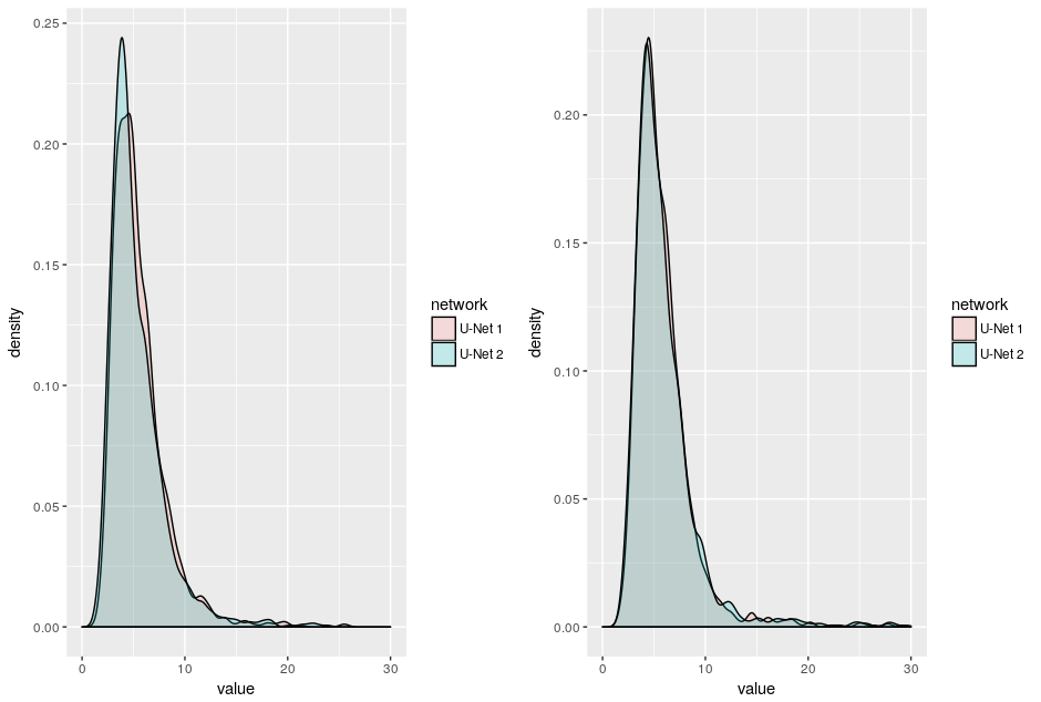
(b) $d_{H}$ endo / epi

Figure 5: $d_{m}$ and $d_{H}$ overlapping distributions from U-Net 1 and U-Net 2

VIII Additional tests performed on ACNNs

VIII-A Auto-encoder implementation and training

The auto-encoders learn to reconstruct all segmentation masks of the training dataset from a low dimensional vector of fixed size with $32$ values. The detailed architecture is given in table IV. Convolutions are not followed by any padding so the image size is gradually reduced in the encoding part and enlarged in the decoding part. L1 regularization is applied on the code so that code coefficients remain small and of similar magnitude for all auto-encoders. ELU activations are used as they showed to lead to a better convergence.

We train the networks during 50 epochs (long after convergence) with a batch size of 50. Cross-Entropy is used as the loss to optimize with the Adam optimizer and a learning rate of 1e-4. Train, validation and test sets are the same as the corresponding segmentation network and all ten auto-encoders achieve an accuracy superior to 92$\%$.

TABLE IV: AUTO-ENCODER ARCHITECTURE

Level	Layer	Kernel size	Activation
Encoder	Conv	16 (3,3)	eLU
	Conv	16 (3,3)	eLU
	Conv	32 (3,3)	eLU
	Conv	32 (3,3)	eLU
	Conv	64 (3,3)	eLU
	Conv	64 (3,3)	eLU
Code	Conv+Flatten	1 (3,3)	eLU
	Dense	32
Decoder	Dense	169	eLU
	Reshape	1 (13,13)
	ConvTranspose	64 (4,4)	eLU
	ConvTranspose	64 (4,4)	eLU
	Conv	64 (3,3)	eLU
	ConvTranspose	32 (4,4)	eLU
	Conv	32 (3,3)	eLU
	ConvTranspose	16 (4,4)	eLU
	Conv	16 (3,3)	eLU
	ConvTranspose	16 (4,4)	eLU
Seg	Conv	4 (3,3)	Softmax

VIII-B Impact of the regularization loss

The regularization loss corresponds to the mean squared error of the code coefficients. As its values do not scale with the ones provided by the segmentation loss, a multiplying factor is applied. In our study, it is set at $10^{4}$ so that the two losses have close initial values. In Table V, we compare the segmentation accuracy reached by our ACNN implementation for two different values of the regularization weight : the chosen one, and one 100 times stronger. From this table, it can be seen that the increase of the regularization weight affects the quality of the results, especially for the dH metric.

TABLE V: Segmentation accuracy for ACNN architecture with different shape regularization strength

Methods *
	$\boldsymbol{LV\textsubscript{Endo}}$			$\boldsymbol{LV\textsubscript{Epi}}$
	D	dm	dH	D	dm	dH
	val.	mm	mm	val.	mm	mm
ACNN - $\lambda=10^{4}$	0.918	1.8	5.9	0.946	1.9	6.4
	$\pm$0.050	$\pm$1.0	$\pm$3.5	$\pm$0.030	$\pm$1.1	$\pm$4.2
ACNN - $\lambda=10^{6}$	0.912	1.9	6.2	0.947	1.9	6.9
	$\pm 0.054$	$\pm 1.1$	$\pm 4.0$	$\pm 0.030$	$\pm 1.1$	$\pm 5.8$

VIII-C Influence of the training set size

To study the influence of the training set of the auto-encoder and segmentation network of ACNNs, we first trained two auto-encoders using the fold 6 as validation set and fold 5 as test set : SR400 was trained on 400 patients while SR15 was trained on 15 patients from the same training set.

We then trained five ACNN networks (using U-Net 1 for the segmentation part of the network) with the same validation and test set. The $50p\_no\_SR$ model involved no shape regularization and was trained on 50 patients (200 images). The $5p\_no\_SR$ model was trained on a smaller set of only $5$ patients (20 images). Models $50p\_with\_SR15$ and $50p\_with\_SR400$ were trained on the same training set as $50p\_no\_SR$ while optimizing the ACNN shape regularization auxiliary loss returned respectively from the $SR15$ and $SR400$ auto-encoders. Finally, the $5p\_SR400$ model was trained on the same training set as the $5p\_no\_SR$ model, with the shape regularization from $SR400$.

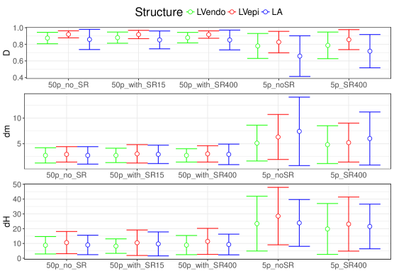
Figure 6: Geometric performance illustrated by standard error bars around the mean values for the 5 segmentation networks.

Fig.6 represent the geometrical results of all five models. It can be observed that : i) Shape regularization does not improve results for an ACNN trained on 50 patients but it does significantly improve the results for a smaller training set of 5 patients; ii) Using for the ACNN an auto-encoder learnt from 15 patients (accuracy of $84\%$) produced close results compared to the one learnt on 400 patients.

These results support the idea that shape regularization will be helpful on datasets for which the training dataset size is not sufficient to learn the annotated shapes’ complexity. For our specific task of 2D echocardiography, it appears that the necessary number of cases is low, inferior to 50 patients, probably because the shape variability is also low, allowing an auto-encoder to roughly infer it from a few number of cases. In the paper experiments, we trained encoder-decoder networks on 400 patients, which explains why the ACNN do not show any significant improvement compared to U-Net 1.

IX Tests on U-Net ++

We provide in table VI a few results obtained from the U-Net ++ architecture, where we studied the influence of averaging the last two segmentation maps and changing the baseline with the succession of layers from U-net 1. Deep Supervision was always applied and no dropout was performed, as it was always detrimental.

TABLE VI: Segmentation accuracy for ACNN architecture with different shape regularization strength

Methods *
	$\boldsymbol{LV\textsubscript{Endo}}$			$\boldsymbol{LV\textsubscript{Epi}}$
	D	dm	dH	D	dm	dH
	val.	mm	mm	val.	mm	mm
U-Net ++ - Mono output	0.909	2.0	6.6	0.941	2.2	7.1
	$\pm$0.063	$\pm$1.6	$\pm$4.8	$\pm$0.033	$\pm$1.2	$\pm$5.0
U-net ++ - 2 outputs	0.905	2.1	7.3	0.936	2.3	8.6
	$\pm 0.070$	$\pm 4.3$	$\pm 7.3$	$\pm 0.040$	$\pm 1.4$	$\pm 6.5$
U-net ++ - U-Net 1	0.915	1.8	6.4	0.942	2.1	7.1
	$\pm 0.055$	$\pm 1.0$	$\pm 4.0$	$\pm 0.030$	$\pm 1.1$	$\pm 4.7$

From table VI, one can observe that averaging the feature maps of the intermediate output (Unet++ - 2 outputs model) worsened the results (especially the standard deviation), showing the uselessness of this operation on our dataset. The best U-Net ++ implementation corresponds to the one keeping the last ouput as final result and replacing the original layers by the design of the U-Net 1 architecture which has been already optimized on the CAMUS dataset. This model was used in all the experiments given in our paper.

X Geometric and clinical scores supplements

X-A Deep learning behavior: Dice box plots

Complementary to the analysis made in section V-B, we provide in Fig.7 the box plots related to the Dice metric. From the derived boxplot, one can see that, unrelated to the structure, the mono and multi-structures approaches produced close results though statistically different. Concerning the effect of poor image quality, the boxplots show that the two different strategies (learning from all the dataset or from the dataset restricted to good and medium quality images) produced results whose differences are statistically unsignificant. From these observations, the same conclusions as the ones made in the paper can be infered: i) learning the segmentation of one structure (e.g. LV Endo ) in the context of the others (e.g. LV Epi & LA) does not improve significantly the Dice results; ii) the $19\%$ (94 patients) of poor image quality do not bring additional information. Outliers are more numerous on the LA, which can be explained by a greater variability in shape and unoptimized acquisitions for this structure.

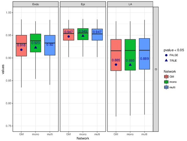
Figure 7: Dice box plots results of the U-Net 1 method for three different schemes (GM for the learning from good & medium image quality, mono for the learning of one structure, multi for the learning of the three structures at the same time). Values in blue displayed under the boxes correspond to mean values computed from each set of measurements. p-values are based on the Wilcoxon signed rank computed with the multi-structures strategy as reference.

X-B Geometric and clinical scores computed on fold $5$

In addition to table III and IV given in the article, we provide in table LABEL:tab:comparison_segmentation_dl_vs_others_fold5 and LABEL:tab:comparison_clinical_indices_dl_vs_others_fold5 of this supplementary material the segmentation accuracy (LV_Endo and LV_Epi) and the clinical scores (LV_EDV, LV_ESV and LV_EF) of the $8$ evaluated methods on fold $5$ restricted to patients having good & medium image quality ($40$ patients). As the results given in the paper, one can see that the EDNs implementations show i) the best segmentation performances on all metrics and structures and ii) the best correlation scores with low biases and standard deviations.

TABLE VII: Segmentation accuracy (LV_Endo and LV_Epi) of $8$ evaluated methods on fold $5$ restricted to good & medium image quality ($40$ patients). The values in bold refer to the best performance for each measure. p-values are based on the Wilcoxon signed rank between the U-Net 1 and 2 methods for each evaluation metric.

Methods *	ED						ES
	$\boldsymbol{LV\textsubscript{Endo}}$			$\boldsymbol{LV\textsubscript{Epi}}$			$\boldsymbol{LV\textsubscript{Endo}}$			$\boldsymbol{LV\textsubscript{Epi}}$
	D	dm	dH	D	dm	dH	D	dm	dH	D	dm	dH
	val.	mm	mm	val.	mm	mm	val.	mm	mm	val.	mm	mm
O1a vs O2	0.919	2.2	6.0	0.913	3.5	8.0	0.873	2.7	6.6	0.890	3.9	8.6
(inter-obs)	$\pm$0.033	$\pm$0.9	$\pm$2.0	$\pm$0.037	$\pm$1.7	$\pm$2.9	$\pm$0.060	$\pm$1.2	$\pm$2.4	$\pm$0.047	$\pm$1.8	$\pm$3.3
O1a vs O3	0.886	3.3	8.2	0.943	2.3	6.5	0.823	4.0	8.8	0.931	2.4	6.4
(inter-obs)	$\pm$0.050	$\pm$1.5	$\pm$2.5	$\pm$0.018	$\pm$0.8	$\pm$2.6	$\pm$0.091	$\pm$2.0	$\pm$3.5	$\pm$0.025	$\pm$1.0	$\pm$2.4
O2 vs O3	0.921	2.3	6.3	0.922	3.0	7.4	0.888	2.6	6.9	0.885	3.9	8.4
(inter-obs)	$\pm$0.037	$\pm$1.2	$\pm$2.5	$\pm$0.036	$\pm$1.5	$\pm$3.0	$\pm$0.058	$\pm$1.3	$\pm$2.9	$\pm$0.054	$\pm$1.9	$\pm$2.8
SRF	0.905	2.4	9.5	0.920	3.0	10.8	0.854	3.0	10.7	0.900	3.3	13.4
	$\pm$0.053	$\pm$1.3	$\pm$6.3	$\pm$0.053	$\pm$1.8	$\pm$7.0	$\pm$0.099	$\pm$1.8	$\pm$8.6	$\pm$0.062	$\pm$1.8	$\pm$9.4
BEASM fully	0.882	3.2	8.5	0.897	3.9	9.9	0.832	3.6	9.3	0.883	4.1	10.4
	$\pm$0.065	$\pm$2.1	$\pm$5.0	$\pm$0.052	$\pm$2.3	$\pm$5.0	$\pm$0.089	$\pm$2.2	$\pm$5.4	$\pm$0.051	$\pm$2.2	$\pm$4.9
BEASM semi	0.922	2.1	5.6	0.916	3.2	7.8	0.868	2.8	7.1	0.904	3.3	8.7
	$\pm$0.031	$\pm$0.8	$\pm$2.0	$\pm$0.040	$\pm$1.6	$\pm$2.8	$\pm$0.057	$\pm$1.2	$\pm$3.1	$\pm$0.036	$\pm$1.4	$\pm$3.0
U-Net 1	0.941	1.5	5.0	0.954	1.7	5.2	0.917	1.6	5.0	0.947	1.8	5.4
	$\pm$0.021	$\pm$0.5	$\pm$1.4	$\pm$0.018	$\pm$0.7	$\pm$1.9	$\pm$0.037	$\pm$0.6	$\pm$2.1	$\pm$0.020	$\pm$0.7	$\pm$2.1
U-Net 2	0.945	1.4	4.9	0.954	1.8	5.7	0.927	1.3	4.9	0.946	1.9	6.0
	$\pm$0.021	$\pm$0.5	$\pm$1.9	$\pm$0.017	$\pm$0.7	$\pm$3.1	$\pm$0.039	$\pm$0.6	$\pm$2.5	$\pm$0.023	$\pm$0.8	$\pm$3.4
ACNN	0.942	1.4	5.0	0.954	1.7	5.5	0.917	1.6	5.0	0.948	1.8	5.9
	$\pm 0.021$	$\pm 0.5$	$\pm 1.5$	$\pm 0.018$	$\pm 0.7$	$\pm 2.3$	$\pm 0.040$	$\pm 0.6$	$\pm 2.0$	$\pm 0.022$	$\pm 0.8$	$\pm 3.1$
SHG	0.941	1.4	5.1	0.952	1.9	5.4	0.918	1.5	4.8	0.944	2.0	5.6
	$\pm 0.024$	$\pm 0.6$	$\pm 2.0$	$\pm 0.019$	$\pm 0.8$	$\pm 2.8$	$\pm 0.04$	$\pm 0.6$	$\pm 1.7$	$\pm 0.025$	$\pm 0.9$	$\pm 2.0$
U-Net ++	0.934	1.6	5.4	0.947	2.0	6.6	0.916	1.5	5.3	0.939	2.1	7.7
	$\pm 0.025$	$\pm 0.6$	$\pm 1.9$	$\pm 0.023$	$\pm 0.9$	$\pm 4.3$	$\pm 0.041$	$\pm 0.7$	$\pm 2.4$	$\pm 0.027$	$\pm 1.1$	$\pm 6.8$
p-values	$\approx 0.053$	$\approx 0.054$	$\approx 0.245$	$\approx 0.710$	$\approx 0.520$	$\approx 0.692$	$\ll 0.05$	$\ll 0.05$	$\approx 0.517$	$\approx 0.926$	$\approx 0.675$	$\approx 0.0988$

TABLE VIII: Clinical metrics of the 8 evaluated methods on fold $5$ restricted to patients having good & medium image quality ($40$ patients in total). The values in bold correspond to the best performance for each measure. p-values are based on the Wilcoxon signed rank between the U-Net 1 and 2 methods for the LV_Endo, LV_Epi and LV_EF.

Methods *	LVEDV			LVESV			LVEF
	corr	bias$\pm\sigma$	mae	corr	bias$\pm\sigma$	mae	corr	bias$\pm\sigma$	mae
	val.	ml	ml	val.	ml	ml	val.	%	%
O1a vs O2 (inter-obs)	0.940	18.7$\pm$12.9	18.7	0.956	18.9$\pm$9.3	18.9	0.801	-9.1$\pm$8.1	10.0
O1a vs O3 (inter-obs)	0.895	39.0$\pm$18.8	39.0	0.860	35.9$\pm$17.1	35.9	0.646	-12.6$\pm$10.0	13.4
O2 vs O3 (inter-obs)	0.926	-20.3$\pm$15.6	21.0	0.916	-17.0$\pm$13.5	17.7	0.569	3.5$\pm$11.0	8.5
SRF	0.843	5.3$\pm$18.6	13.9	0.845	12.4$\pm$15.6	15.9	0.603	-11.9$\pm$10.8	13.1
BEASM fully	0.809	19.1$\pm$23.3	21.3	0.791	23.2$\pm$20.6	24.0	0.776	-12.1$\pm$8.2	12.6
BEASM semi	0.913	12.0$\pm$15.4	15.3	0.875	16.3$\pm$15.1	18.0	0.853	-10.2$\pm$6.7	10.5
U-Net 1	0.973	-7.7$\pm$8.3	8.7	0.945	-3.1$\pm$10.1	7.6	0.820	-2.6$\pm$7.5	5.9
U-Net 2	0.977	-4.0 $\pm$7.3	6.6	0.976	-0.9$\pm$ 7.0	5.2	0.928	-2.3$\pm$4.8	4.0
ACNN	0.970	-3.3$\pm$ 8.4	6.3	0.943	0.8$\pm 9.9$	7.0	0.851	-3.9$\pm$6.8	6.5
SHG	0.967	-3.1$\pm$8.5	6.6	0.947	0.7$\pm$9.6	7.0	0.842	-3.9$\pm$6.9	6.3
U-Net ++	0.971	-11.5$\pm$ 9.0	12.0	0.963	-5.7$\pm$ 9.5	7.9	0.872	-2.0$\pm$ 6.3	4.7
p-values	$<0.05$			$\ll 0.05$			$\ll 0.05$
* LVEDV: End diastolic left ventricular volume; LVESV: End systolic left ventricular volume;
corr: Pearson correlation coefficient; mae: mean absolute error.

X-C Geometric scores computed on the poor quality images ($94$ patients)

In addition to table III given in the article, we provide in table LABEL:tab:comparison_segmentation_dl_vs_others_poor_quality_images of this supplementary material the segmentation accuracy (LV_Endo and LV_Epi) of the $8$ evaluated methods on the ten test sets restricted to patients having poor image quality ($94$ patients). As the results given in the paper, one can see that the EDNs architectures show the best segmentation performances on all metrics and structures except for the $d_{H}$ metric of the LV_Endo  at ED.

TABLE IX: Segmentation accuracy (LV_Endo and LV_Epi) of $8$ evaluated methods on the ten test datasets restricted to patients having poor image quality ($94$ patients in total). The values in bold refer to the best performance for each measure. p-values are based on the Wilcoxon signed rank between the U-Net methods for each evaluation metric.

Methods *	ED						ES
	$\boldsymbol{LV\textsubscript{Endo}}$			$\boldsymbol{LV\textsubscript{Epi}}$			$\boldsymbol{LV\textsubscript{Endo}}$			$\boldsymbol{LV\textsubscript{Epi}}$
	D	dm	dH	D	dm	dH	D	dm	dH	D	dm	dH
	val.	mm	mm	val.	mm	mm	val.	mm	mm	val.	mm	mm
SRF	0.869	3.6	14.3	0.891	4.2	15.9	0.801	4.6	17.0	0.852	4.9	18.0
	$\pm$0.062	$\pm$2.0	$\pm$9.4	$\pm$0.063	$\pm$2.4	$\pm$8.5	$\pm$0.123	$\pm$3.5	$\pm$13.2	$\pm$0.112	$\pm$3.1	$\pm$12.1
BEAS fully	0.857	4.1	10.5	0.888	4.5	11.9	0.801	4.7	12.3	0.873	4.7	12.4
	$\pm$0.083	$\pm$2.6	$\pm$6.3	$\pm$0.058	$\pm$2.6	$\pm$6.2	$\pm$0.102	$\pm$2.7	$\pm$6.6	$\pm$0.063	$\pm$2.6	$\pm$6.2
BEAS semi	0.915	2.4	6.4	0.914	3.4	8.5	0.859	3.3	8.3	0.900	3.6	9.5
	$\pm$0.039	$\pm$1.2	$\pm$2.7	$\pm$0.035	$\pm$1.5	$\pm$2.9	$\pm$0.063	$\pm$1.6	$\pm$3.6	$\pm$0.039	$\pm$1.6	$\pm$3.4
U-Net 1	0.921	2.1	6.5	0.945	2.2	6.8	0.893	2.2	6.8	0.935	2.4	7.2
	$\pm$0.037	$\pm$1.0	$\pm$3.0	$\pm$0.021	$\pm$1.0	$\pm$3.0	$\pm$0.059	$\pm$1.2	$\pm$4.2	$\pm$0.031	$\pm$1.3	$\pm$4.7
U-Net 2	0.921	2.1	6.8	0.947	2.1	7.2	0.898	2.1	6.6	0.937	2.2	7.6
	$\pm$0.037	$\pm$1.0	$\pm$3.3	$\pm$0.023	$\pm$1.0	$\pm$3.8	$\pm$0.057	$\pm$1.2	$\pm$3.6	$\pm$0.032	$\pm$1.2	$\pm$4.8
ACNN	0.915	2.2	7.2	0.939	2.4	8.0	0.885	2.4	7.3	0.929	2.5	8.0
	$\pm 0.041$	$\pm 1.1$	$\pm 3.7$	$\pm 0.027$	$\pm 1.2$	$\pm 5.5$	$\pm 0.059$	$\pm 1.2$	$\pm 4.3$	$\pm 0.034$	$\pm 1.3$	$\pm 4.7$
SHG	0.919	2.1	6.8	0.943	2.3	7.1	0.889	2.3	7.0	0.934	2.4	7.3
	$\pm 0.041$	$\pm 1.2$	$\pm 3.9$	$\pm 0.026$	$\pm 1.2$	$\pm 4.0$	$\pm 0.057$	$\pm 1.2$	$\pm 4.0$	$\pm 0.032$	$\pm 1.3$	$\pm 4.6$
U-Net ++	0.910	2.3	7.9	0.938	2.5	8.8	0.886	2.3	7.9	0.924	2.7	9.6
	$\pm 0.041$	$\pm 1.1$	$\pm 3.8$	$\pm 0.028$	$\pm 1.2$	$\pm 5.1$	$\pm 0.084$	$\pm 1.4$	$\pm$ 5.5	$\pm 0.036$	$\pm 1.4$	$\pm$ 7.2
p-values	$\approx 0.939$	$\approx 0.656$	$\approx 0.409$	$\approx 0.054$	$\approx 0.088$	$\approx 0.541$	$\approx 0.194$	$\approx 0.177$	$\approx 0.708$	$\approx 0.061$	$\approx 0.059$	$\approx 0.278$

From these results, one can see that the performances of all the algorithms (except the SRF) remain close to their corresponding results on good and medium image quality (table III in the article). This suggests that the image quality criteria does not influence so much the quality of the results of automatic solutions. This observation is especially true for encoder-decoder networks since they show less performance drop compared to the non-deep learning techniques. P-values indicate that on this test set of 94 patients, the differences between U-Net 1 and U-Net 2 predictions are not significant.

X-D Bland Altman plots of the LV_EF scores

As complements to the results given in table IV of the article, we provide in Fig. 8 and 9 the Bland Altman plots of the LV_EF measurements between the three cardiologists (inter-variability) and the two set of annotations from the first cardiologist (intra-variability), as well as for the $8$ evaluated methods. For a good visualization and an easy comparison, results are shown for errors between -40 and 40.

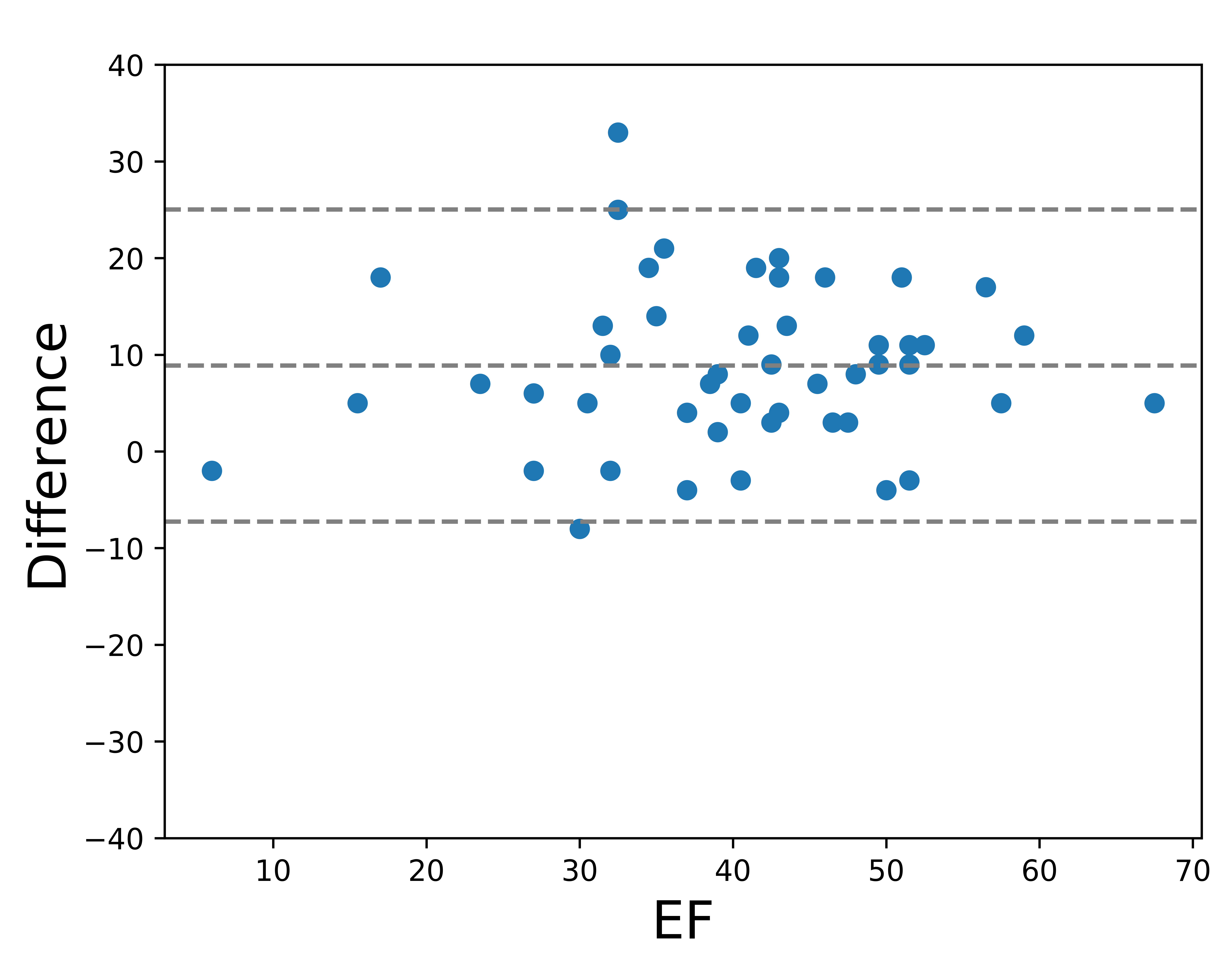
(a) O₂ vs O_1a

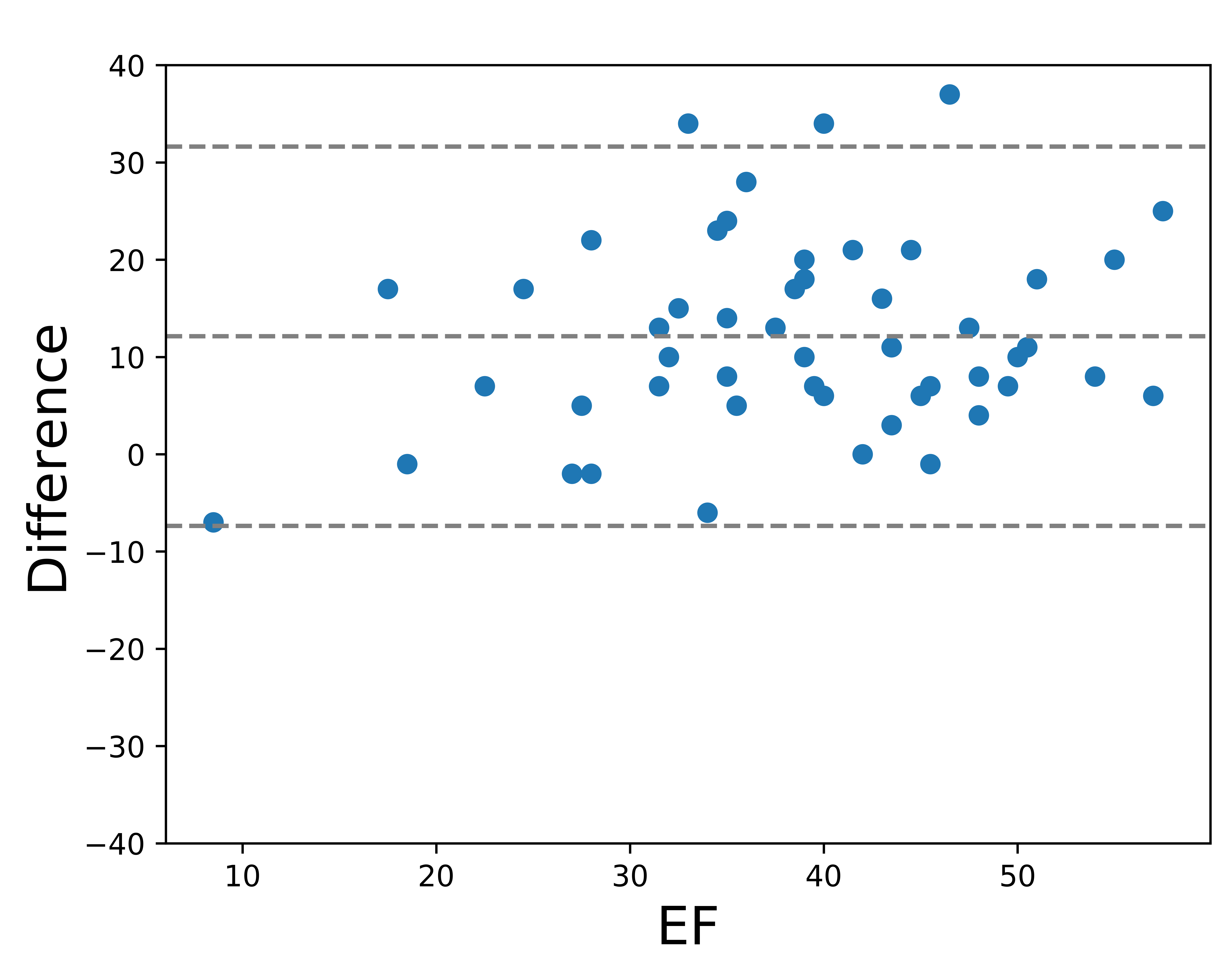
(b) O₃ vs O_1a

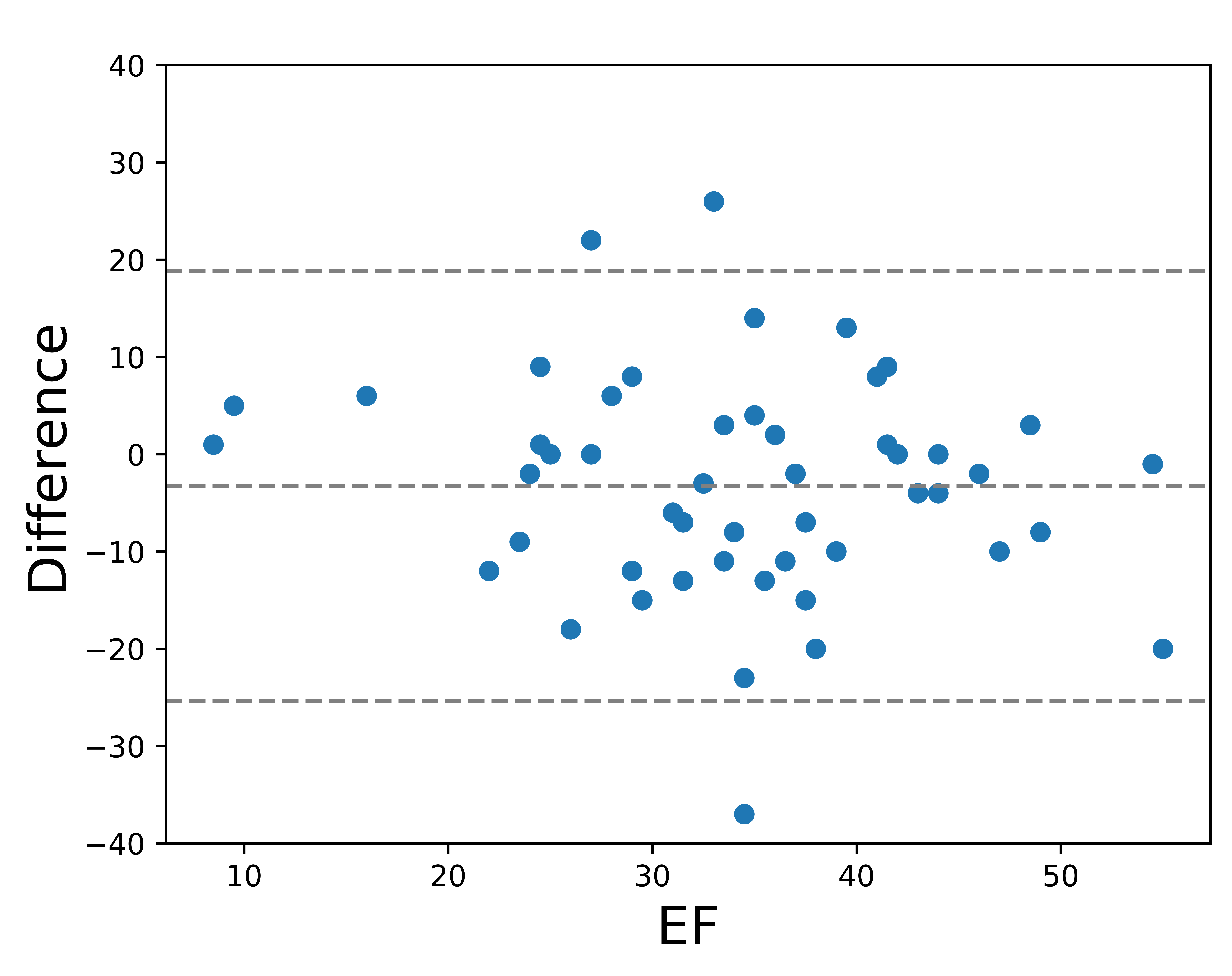
(c) O₃ vs O₂

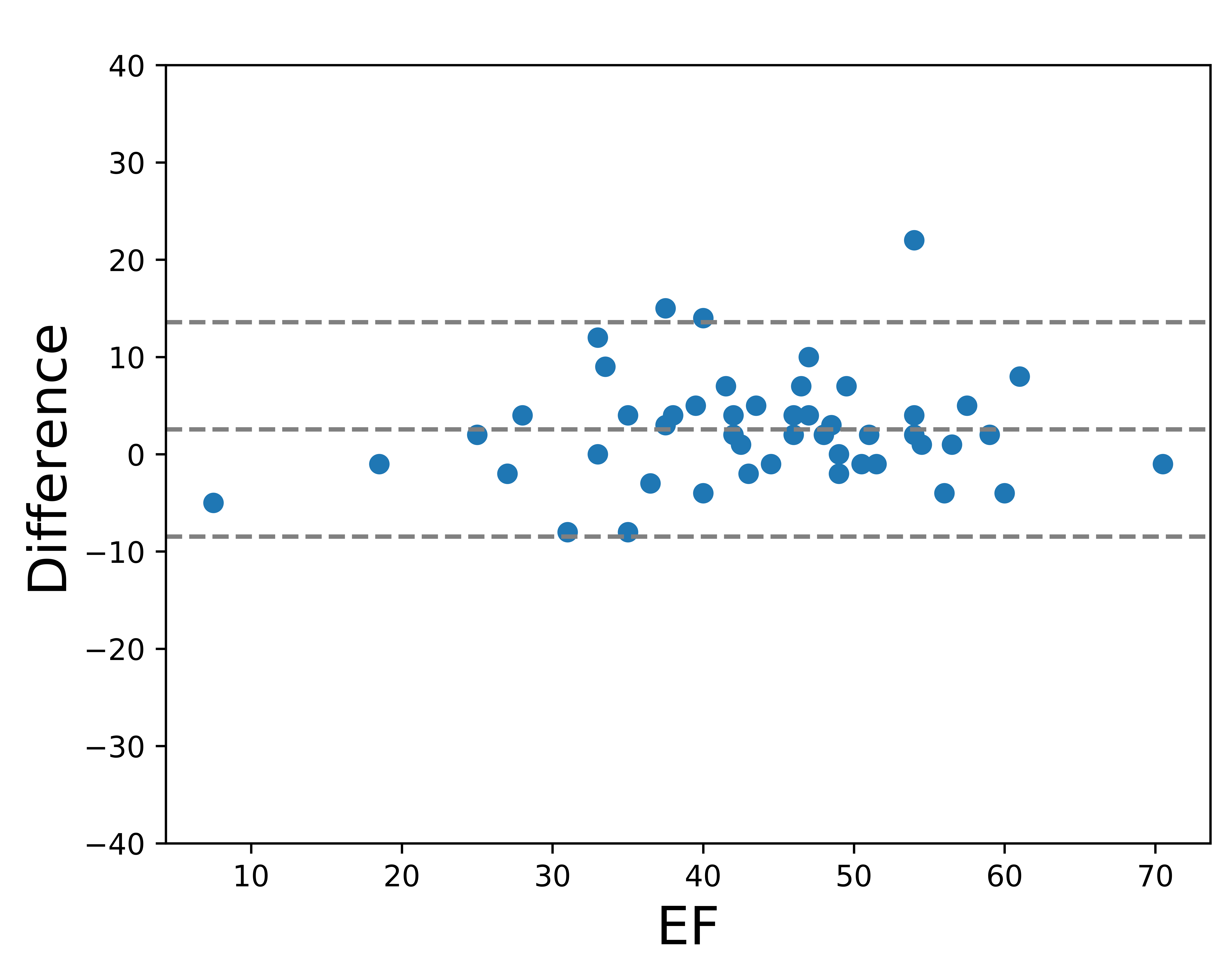
(d) O_1b vs O_1a

Figure 8: Bland Altman plots of the LV_EF scores computed between the cardiologists from fold $5$

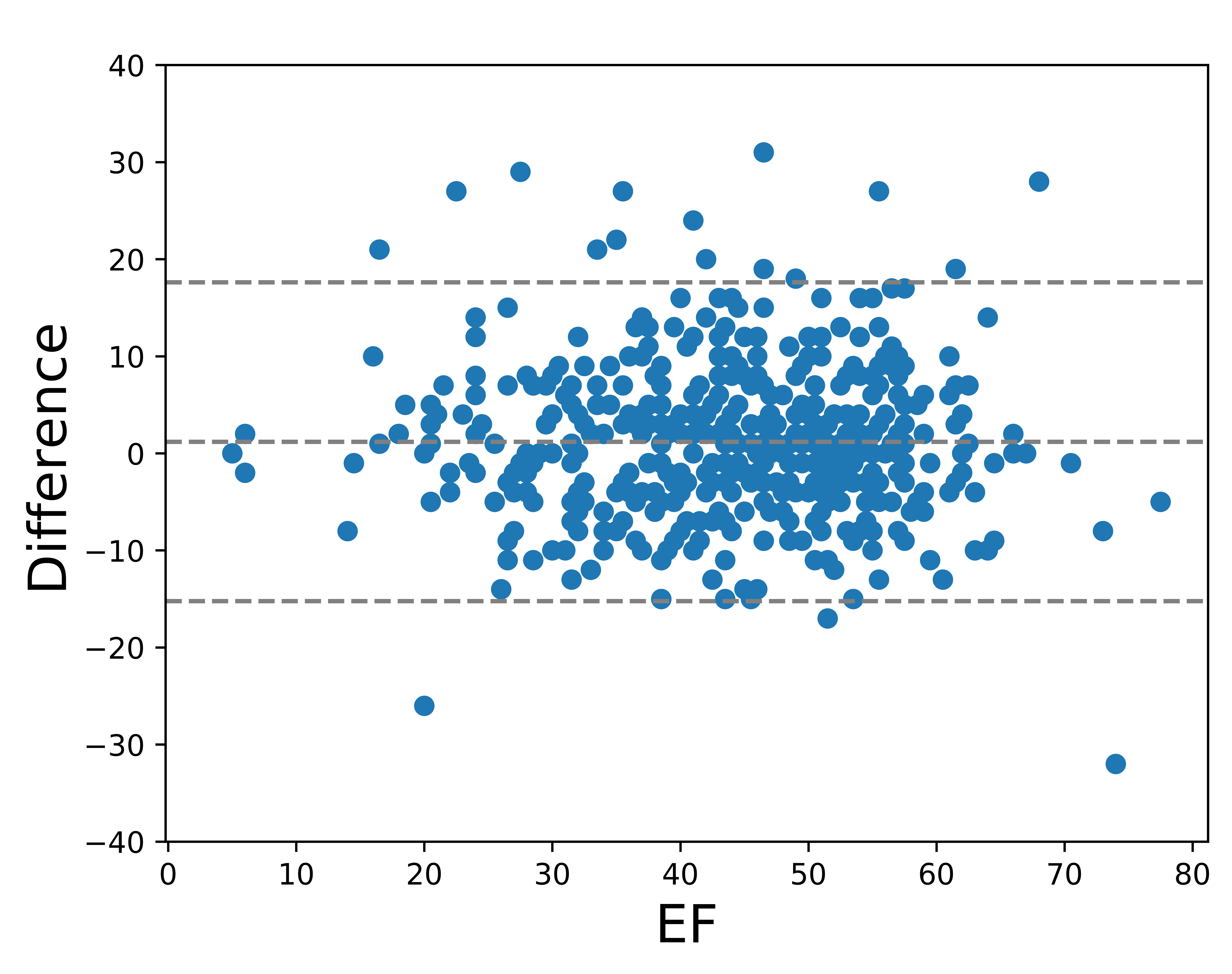
(a) U-Net 1 vs O_1a

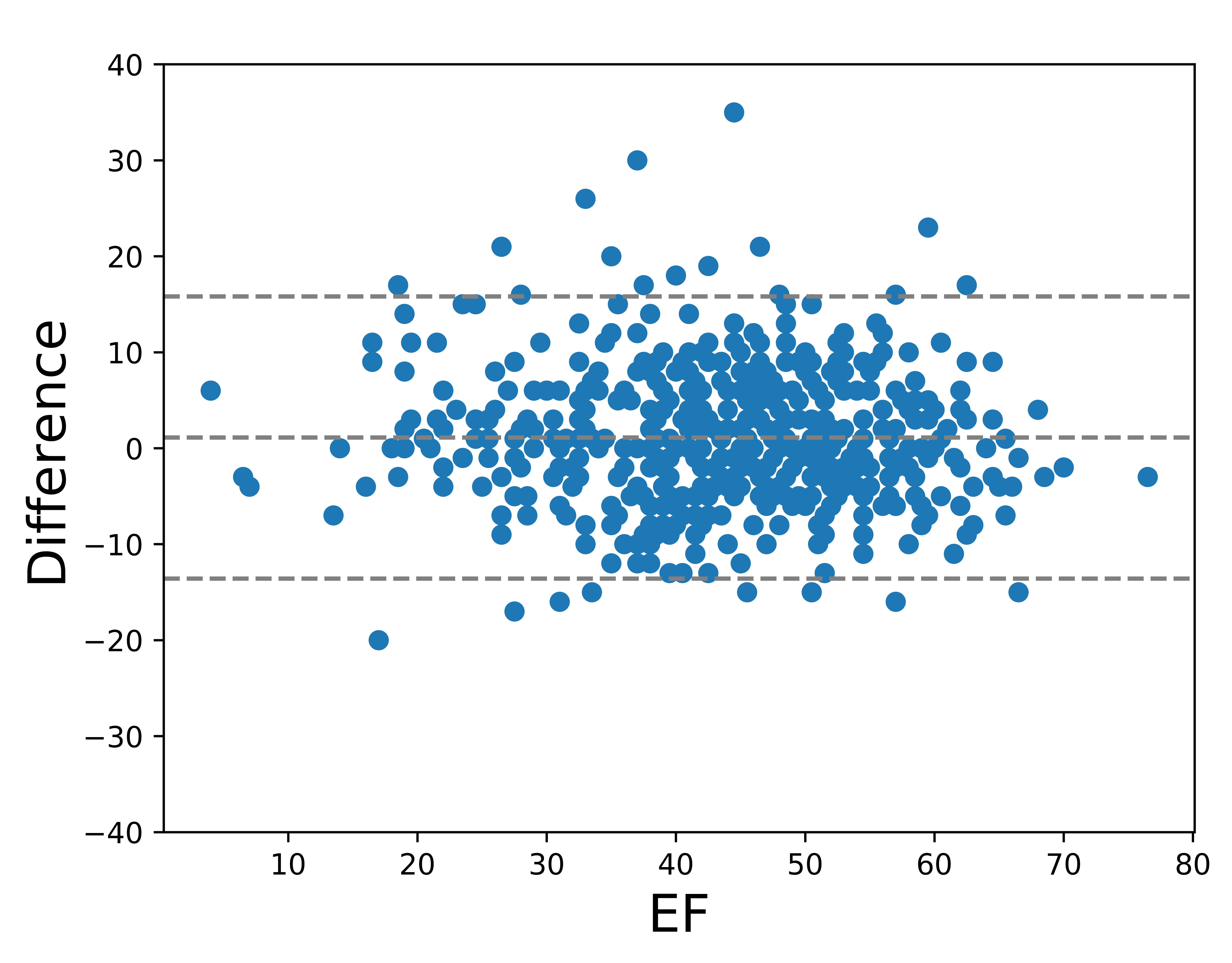
(b) U-Net 2 vs O_1a

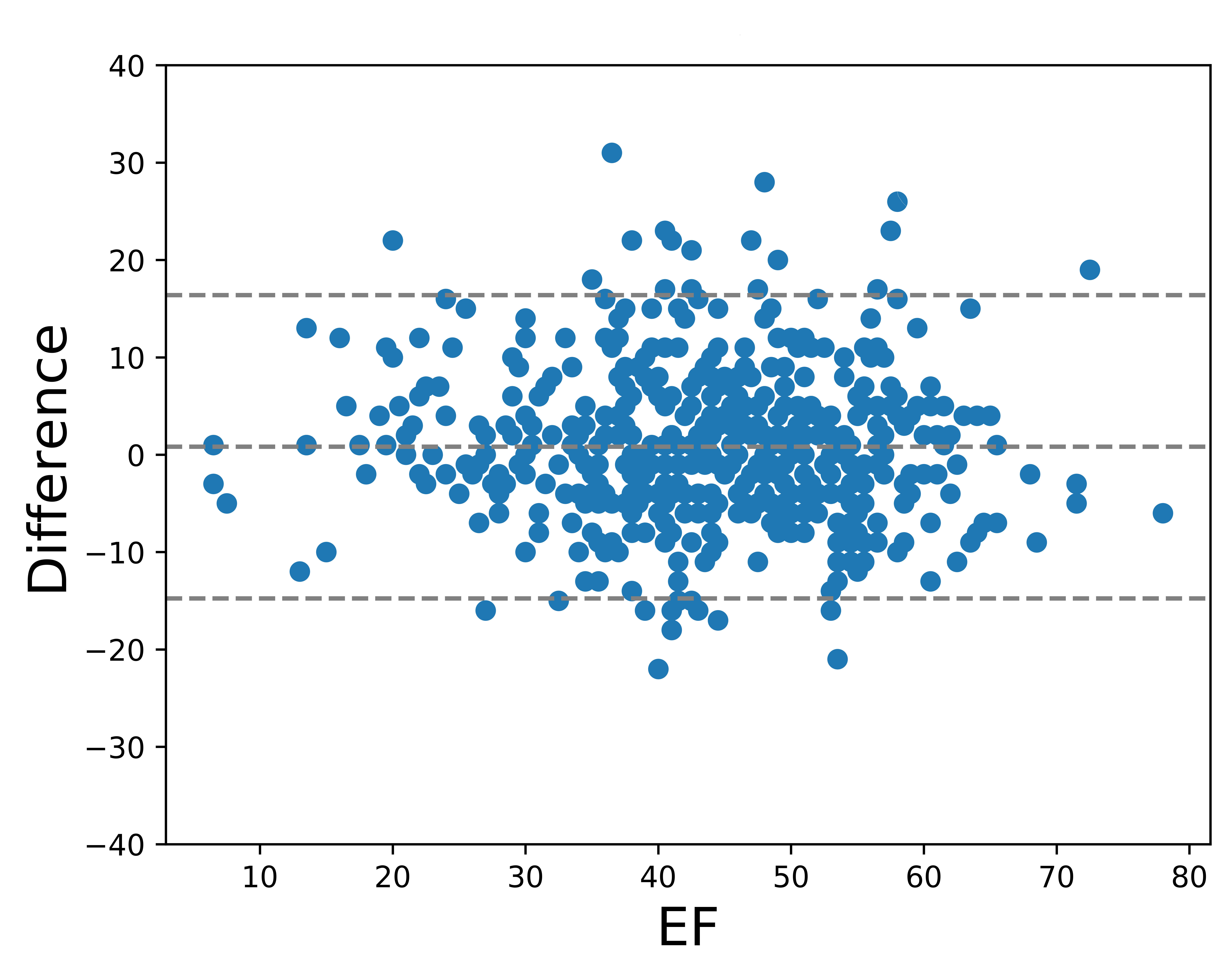
(c) ACNN vs O_1a

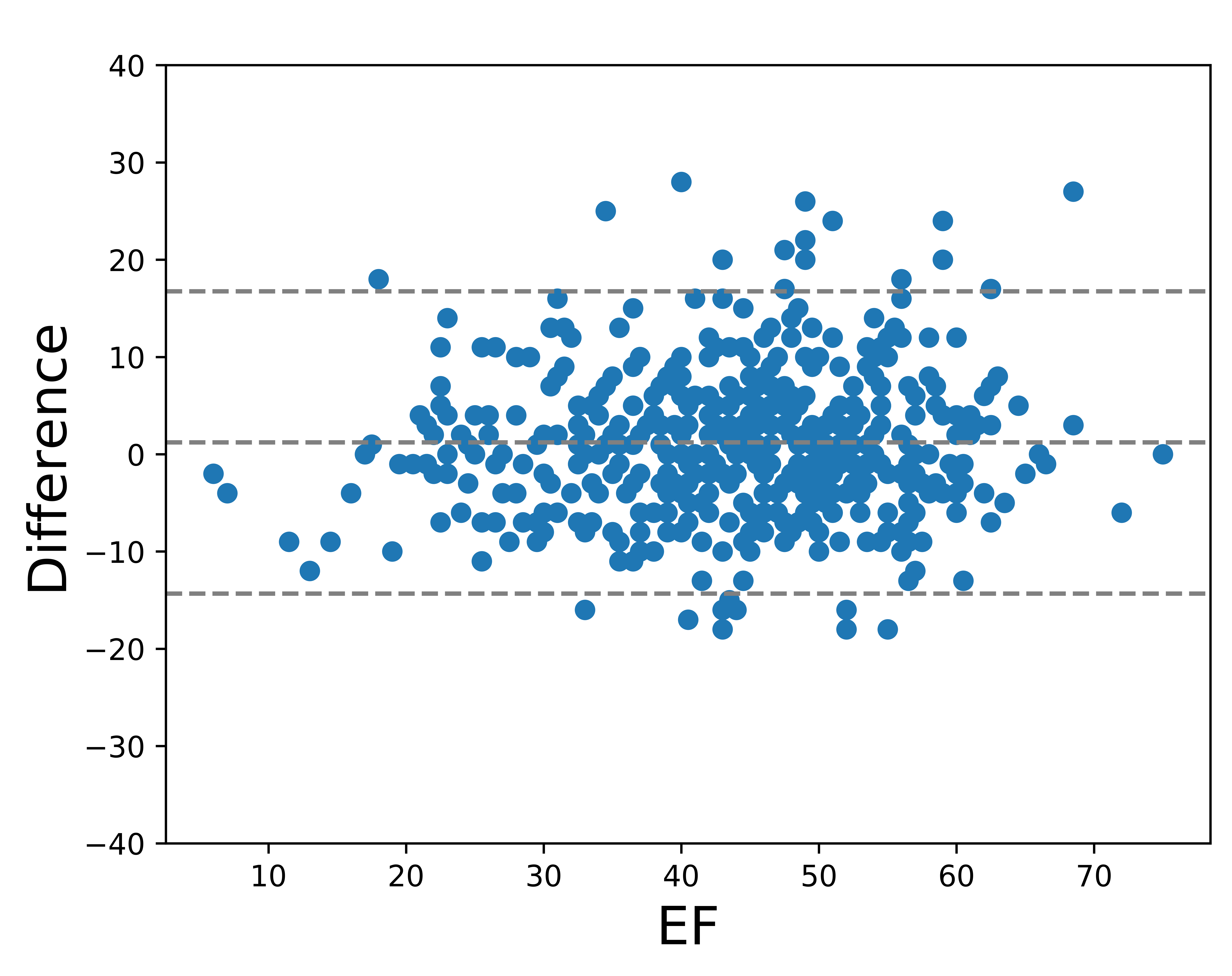
(d) SHG vs O_1a

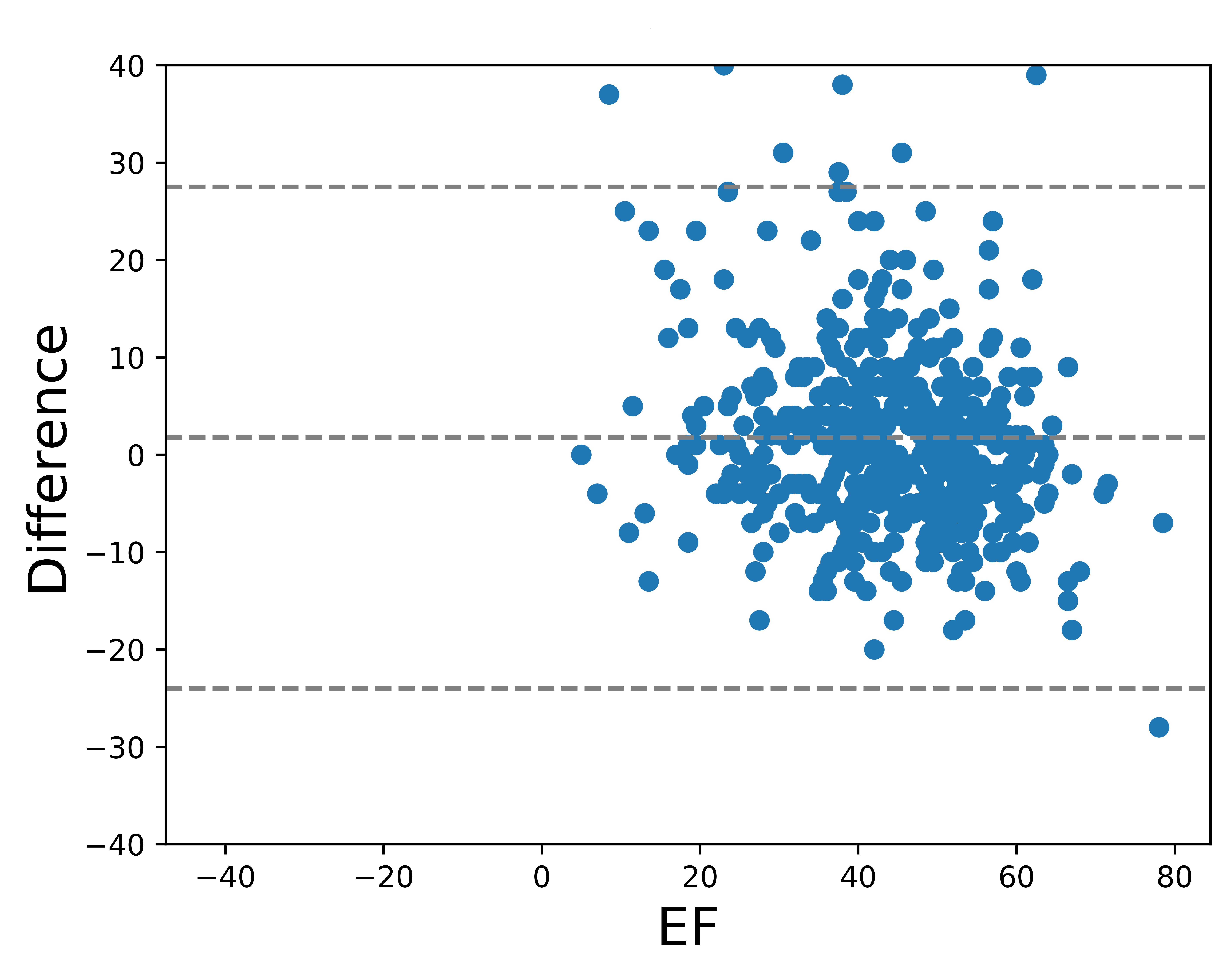
(e) U-Net ++ vs O_1a

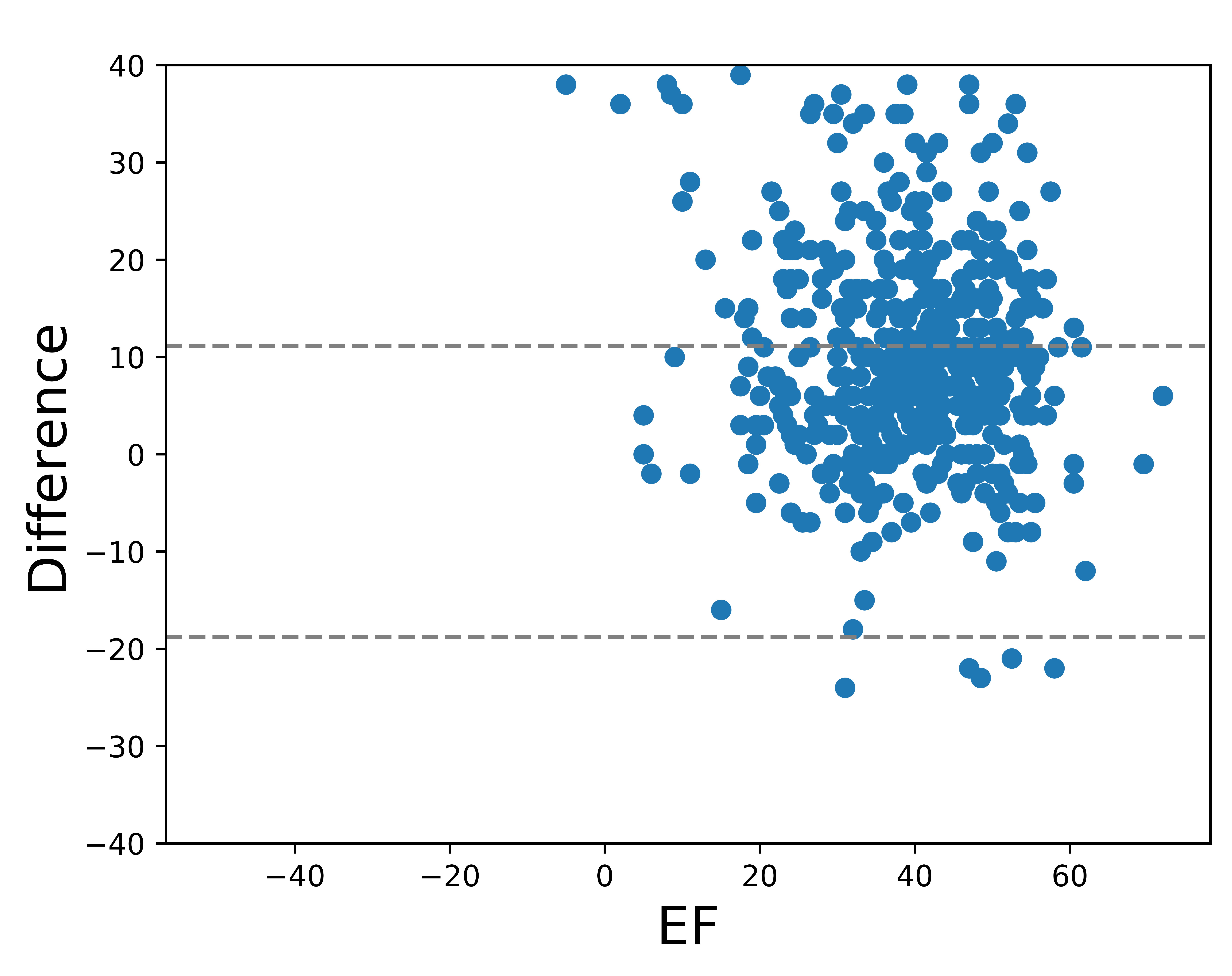
(f) SRF vs O_1a

(g) BEASM-auto vs O_1a

(h) BEASM-semi vs O_1a

Figure 9: Bland Altman plots of the LV_EF scores computed for the $8$ evaluated methods from the full dataset. Mean difference and $95\%$ confidence interval are represented with dotted horizontal lines.

XI Additional insights on outliers

XI-A Influence of the size of the training dataset

In complement to Section VI of the article, Fig. 10 show the evolution of the number of outliers derived from the U-Net 1 model on fold 5 when gradually increasing the training dataset, considering only images of good and medium image quality :

Figure 10: Number of outliers (in % of the CAMUS dataset) produced on fold 5 restricted to patients having good or medium image quality for different training set size.

Interestingly, while the improvement between 50 to 200 patients is quite pronounced (e.g. of the outliers rate from $34\%$ to $13\%$), one can observe a change in the evolution of the performance of the U-Net 1 method for more than 200 patients. Indeed, from this value on, the outliers rate seems to stabilize around 12-13$\%$. These results confirm the observations made from Figure 3 of the article, i.e. the U-Net 1 method needs a training dataset of at least 200 patients to reach highly competitive results, which can slightly be further improved with an even larger training dataset.

XI-B Comparison between methods

As complement, we provide in table LABEL:tab:outliers the outliers rate produced by each of the 8 methods as well as by each expert (using cardiologist $O1_{a}$ as reference) on fold 5, for patients having good & medium image quality (40 patients).

TABLE X: Outliers rate of the 8 methods compared to Observer $O_{1a}$ on the whole dataset and to the cardiologists on the fifth fold, restricted to patients having good & medium image quality (respectively 406 and 40 patients in total).

Outliers	SRF	BEASM-fully	BEASM-semi	U-Net 1	U-Net 2	ACNN	SHG	U-net ++	$O_{2}$	$O_{3}$	$O_{2}|O_{3}$	$O_{1b}$
	69%	79%	59%	18%	18%	22%	18%	30%	56%	58%	46%	13%

XII Visual assessment of the obtained segmentation results

Fig. 11 provides the segmentation results obtained from U-Net1 on a patient with medium quality. This case has been chosen since it reflect on at least one image the median scores obtained by the U-Net 1 algorithm on the full dataset for the endocardium and epicardium: $d_{m}$-endo = 1.6 mm, $d_{m}$-epi = 1.7 mm.

(a) $2$CH-ED: $d_{m}$-endo = 1.0 , $d_{m}$-epi = 2.2 , $d_{H}$-endo = 4.2 , $d_{H}$-epi = 7.1 mm.

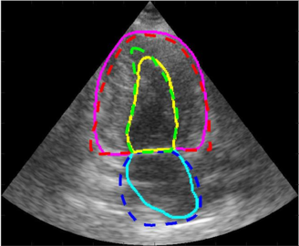
(b) $2$CH-ES: $d_{m}$-endo = 1.3 , $d_{m}$-epi = 2.8 , $d_{H}$-endo = 7.8 , $d_{H}$-epi = 8.3 mm.

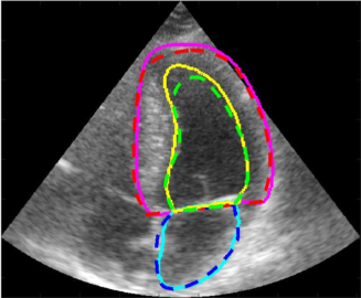
(c) $4$CH-ED: $d_{m}$-endo = 1.7 , $d_{m}$-epi = 1.7 , $d_{H}$-endo = 6.3 , $d_{H}$-epi = 4.0 mm.

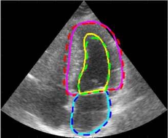
(d) $4$CH-ES: $d_{m}$-endo = 1.5 , $d_{m}$-epi = 1.5 , $d_{H}$-endo = 5.9 , $d_{H}$-epi = 3.7 mm.

Figure 11: Segmentation results obtained by the U-Net 1 architecture on Patient 252 (image defined as medium quality). Ground-truth contours are dotted and prediction contours are drawn in full line.

To allow visual assessment of the segmentation performance of the different methods implemented in our paper, we provide in Fig. 12 to 21 the segmentations results obtained by each of the presented methods and the cardiologists on a given patient with a good image quality.

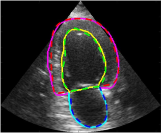
(a) $2$CH-ED: $d_{m}$-endo = 1.4 , $d_{m}$-epi = 1.5 , $d_{H}$-endo = 4.4 , $d_{H}$-epi = 4.8 mm.

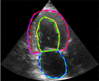
(b) $2$CH-ES: $d_{m}$-endo = 1.6 , $d_{m}$-epi = 2.4 , $d_{H}$-endo = 5.1 , $d_{H}$-epi = 7.7 mm.

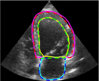
(c) $4$CH-ED: $d_{m}$-endo = 1.0 , $d_{m}$-epi = 2.2 , $d_{H}$-endo = 5.9 , $d_{H}$-epi = 4.5 mm.

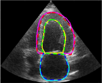
(d) $4$CH-ES: $d_{m}$-endo = 1.0 , $d_{m}$-epi = 1.7 , $d_{H}$-endo = 3.8 , $d_{H}$-epi = 4.5 mm.

Figure 12: Segmentation results obtained by the U-Net 1 architecture on Patient 27 (image defined as good quality). Ground-truth contours are dotted and prediction contours are drawn in full line.

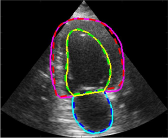
(a) $2$CH-ED : $d_{m}$-endo = 1.1 , $d_{m}$-epi = 1.4 , $d_{H}$-endo = 4.0 , $d_{H}$-epi = 4.0 mm.

(b) $2$CH-ES: $d_{m}$-endo = 1.4 , $d_{m}$-epi = 1.2 , $d_{H}$-endo = 4.4 , $d_{H}$-epi = 4.33 mm.

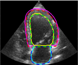
(c) $4$CH-ED: $d_{m}$-endo = 1.6 , $d_{m}$-epi = 2.0 , $d_{H}$-endo = 6.8 , $d_{H}$-epi = 4.6 mm.

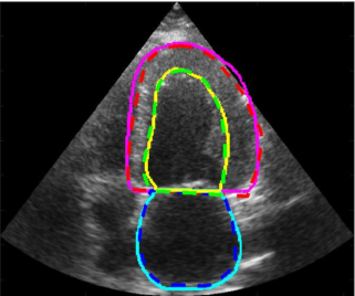
(d) $4$CH-ES: $d_{m}$-endo = 1.6 , $d_{m}$-epi = 1.5 , $d_{H}$-endo = 4.7 , $d_{H}$-epi = 4.3 mm.

Figure 13: Segmentation results obtained by the U-Net 2 architecture on Patient 27.

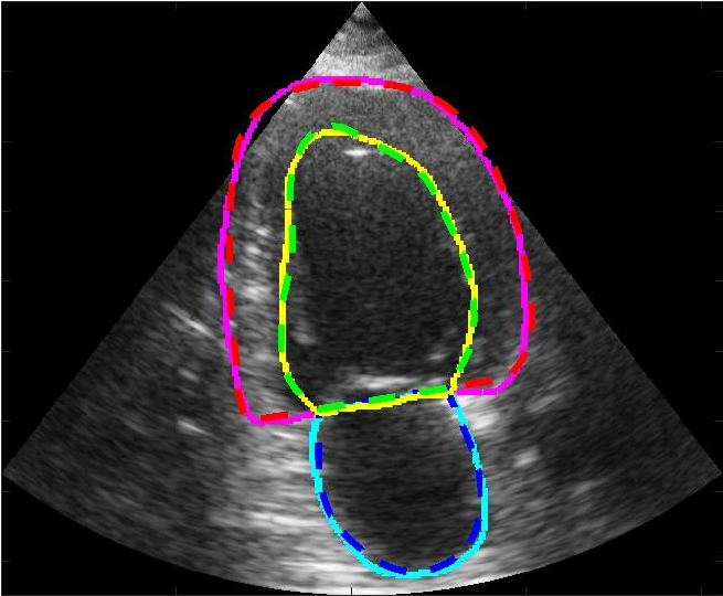
(a) $2$CH-ED : $d_{m}$-endo = 0.7 , $d_{m}$-epi = 1.1 , $d_{H}$-endo = 2.7 , $d_{H}$-epi = 3.3 mm.

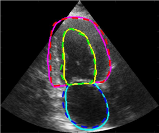
(b) $2$CH-ES: $d_{m}$-endo = 1.2 , $d_{m}$-epi = 1.5 , $d_{H}$-endo = 4.0 , $d_{H}$-epi = 4.0 mm.

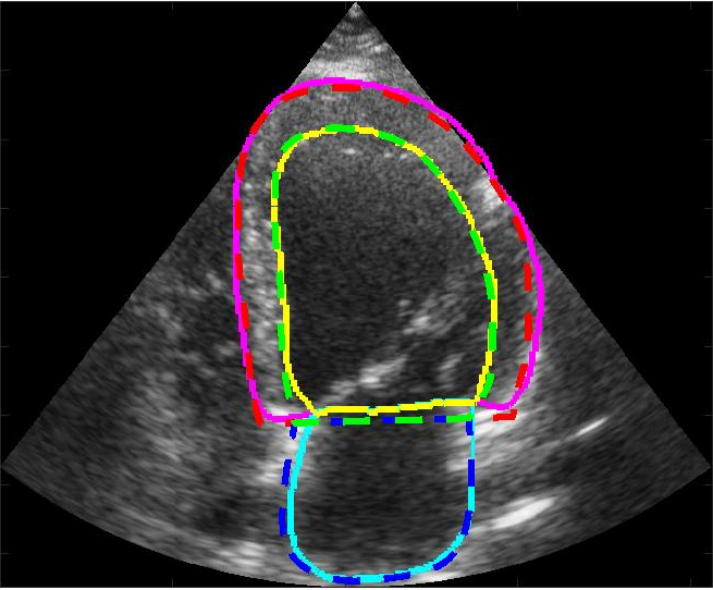
(c) $4$CH-ED: $d_{m}$-endo = 1.2 , $d_{m}$-epi = 1.7 , $d_{H}$-endo = 5.9 , $d_{H}$-epi = 5.1 mm.

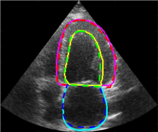
(d) $4$CH-ES: $d_{m}$-endo = 1.3 , $d_{m}$-epi = 1.3 , $d_{H}$-endo = 3.7 , $d_{H}$-epi = 3.7 mm.

Figure 14: Segmentation results obtained by the U-Net 1 ACNN architecture on Patient 27.

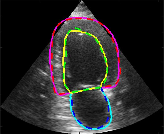
(a) $2$CH-ED : $d_{m}$-endo = 1.1 , $d_{m}$-epi = 1.1 , $d_{H}$-endo = 4.0 , $d_{H}$-epi = 3.1 mm.

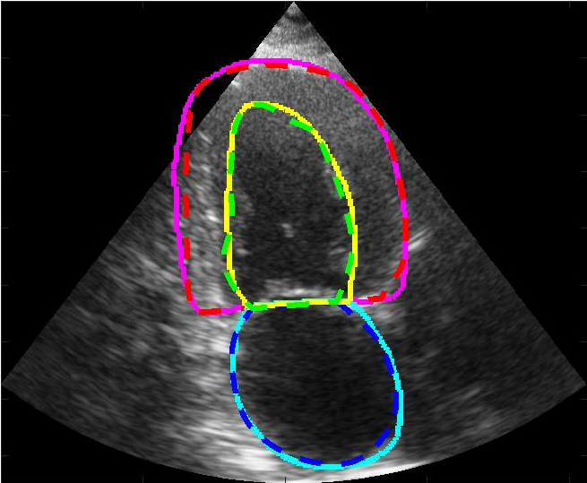
(b) $2$CH-ES : $d_{m}$-endo = 1.2 , $d_{m}$-epi = 1.4 , $d_{H}$-endo = 4.1 , $d_{H}$-epi = 4.7 mm.

(c) $4$CH-ED : $d_{m}$-endo = 1.1 , $d_{m}$-epi = 6.3 , $d_{H}$-endo = 2.7 , $d_{H}$-epi = 5.1 mm.

(d) $4$CH-ES : $d_{m}$-endo = 1.5 , $d_{m}$-epi = 5.5 , $d_{H}$-endo = 1.6 , $d_{H}$-epi = 4.1 mm.

Figure 15: Segmentation results obtained by the U-Net 1 SHG architecture on Patient 27.

(a) $2$CH-ED : $d_{m}$-endo = 1.3 , $d_{m}$-epi = 1.7 , $d_{H}$-endo = 3.7 , $d_{H}$-epi = 4.6 mm.

(b) $2$CH-ES : $d_{m}$-endo = 1.8 , $d_{m}$-epi = 1.7 , $d_{H}$-endo = 4.9 , $d_{H}$-epi = 5.2 mm.

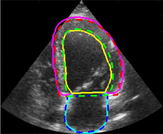
(c) $4$CH-ED : $d_{m}$-endo = 2.5 , $d_{m}$-epi = 2.2 , $d_{H}$-endo = 6.3 , $d_{H}$-epi = 4.7 mm.

(d) $4$CH-ES : $d_{m}$-endo = 1.4 , $d_{m}$-epi = 1.9 , $d_{H}$-endo = 4.1 , $d_{H}$-epi = 4.8 mm.

Figure 16: Segmentation results obtained by the U-Net 1 ++ architecture on Patient 27.

(a) $2$CH-ED: $d_{m}$-endo = 2.7 , $d_{m}$-epi = 1.8 , $d_{H}$-endo = 8.5 , $d_{H}$-epi = 8.1 mm.

(b) $2$CH-ES: $d_{m}$-endo = 3.8 , $d_{m}$-epi = 2.6 , $d_{H}$-endo = 14.0 , $d_{H}$-epi = 7.0 mm.

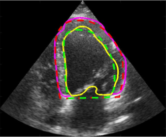
(c) $4$CH-ED: $d_{m}$-endo = 2.3 , $d_{m}$-epi = 2.3 , $d_{H}$-endo = 11.1 , $d_{H}$-epi = 14.2 mm.

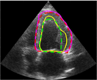
(d) $4$CH-ES: $d_{m}$-endo = 3.2 , $d_{m}$-epi = 1.7 , $d_{H}$-endo = 6.8 , $d_{H}$-epi = 4.8 mm.

Figure 17: Segmentation results obtained by the SRF method on Patient 27.

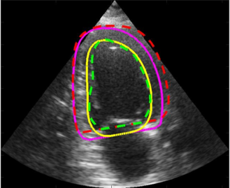
(a) $2$CH-ED: $d_{m}$-endo = 3.0 , $d_{m}$-epi = 3.6 , $d_{H}$-endo = 7.2 , $d_{H}$-epi = 7.7 mm.

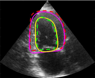
(b) $2$CH-ES: $d_{m}$-endo = 2.9 , $d_{m}$-epi = 2.8 , $d_{H}$-endo = 4.7, $d_{H}$-epi = 5.5 mm.

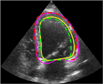
(c) $4$CH-ED: $d_{m}$-endo = 2.4 , $d_{m}$-epi = 1.7 , $d_{H}$-endo = 6.2 , $d_{H}$-epi = 6.6 mm.

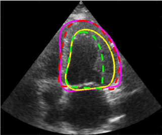
(d) $4$CH-ES: $d_{m}$-endo = 5.0 , $d_{m}$-epi = 2.3 , $d_{H}$-endo = 14.2 , $d_{H}$-epi = 6.5 mm.

Figure 18: Segmentation results obtained by the BEASM method with automatic initialisation on Patient 27.

(a) $2$CH-ED: $d_{m}$-endo = 1.7 , $d_{m}$-epi = 4.9 , $d_{H}$-endo = 4.1 , $d_{H}$-epi = 9.6 mm.

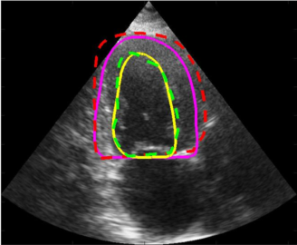
(b) $2$CH-ES: $d_{m}$-endo = 1.5 , $d_{m}$-epi = 3.8 , $d_{H}$-endo = 8.5 , $d_{H}$-epi = 8.5 mm.

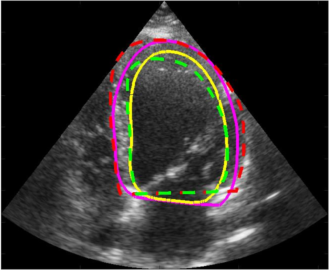
(c) $4$CH-ED: $d_{m}$-endo = 2.1 , $d_{m}$-epi = 3.2 , $d_{H}$-endo = 6.2 , $d_{H}$-epi = 8.2 mm.

(d) $4$CH-ES: $d_{m}$-endo = 3.4 , $d_{m}$-epi = 2.8 , $d_{H}$-endo = 3.5 , $d_{H}$-epi = 7.7 mm.

Figure 19: Segmentation results obtained by the BEASM method with semi-automatic initialisation on Patient 27.

(a) $2$CH-ED: $d_{m}$-endo = 3.1 , $d_{m}$-epi = 4.2 , $d_{H}$-endo = 5.9 , $d_{H}$-epi = 9.0 mm.

(b) $2$CH-ES: $d_{m}$-endo = 3.3 , $d_{m}$-epi = 5.5 , $d_{H}$-endo = 8.1 , $d_{H}$-epi = 9.5 mm.

(c) $4$CH-ED: $d_{m}$-endo = 2.0 , $d_{m}$-epi = 1.4, $d_{H}$-endo = 4.8 , $d_{H}$-epi = 3.4 mm.

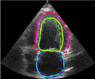
(d) $4$CH-ES: $d_{m}$-endo = 2.4 , $d_{m}$-epi = 1.9 , $d_{H}$-endo = 6.1 , $d_{H}$-epi = 9.0 mm.

Figure 20: Segmentation results obtained by the cardiologist 2 on Patient 27.

(a) $2$CH-ED: $d_{m}$-endo = 4.5 , $d_{m}$-epi = 4.1 , $d_{H}$-endo = 9.7 , $d_{H}$-epi = 4.1 mm.

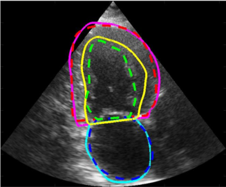
(b) $2$CH-ES: $d_{m}$-endo = 5.9 , $d_{m}$-epi = 4.5 , $d_{H}$-endo = 13.2 , $d_{H}$-epi = 4.5 mm.

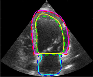
(c) $4$CH-ED: $d_{m}$-endo = 1.7 , $d_{m}$-epi = 4.0 , $d_{H}$-endo = 6.8 , $d_{H}$-epi = 4.0 mm.

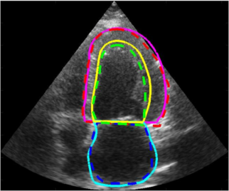
(d) $4$CH-ES: $d_{m}$-endo = 2.7 , $d_{m}$-epi = 4.4 , $d_{H}$-endo = 4.9 , $d_{H}$-epi = 4.4 mm.

Figure 21: Segmentation results obtained by the cardiologist 3 on Patient 27.

XII-A Unsolved cases and limitations

In this section, we show outliers predictions for the U-Net 1 algorithm. Outliers were deemed to constitute $18\%$ of the dataset. Among them, most (about $90\%$) could be associated to anatomically plausible LV and myocardium shapes, but on the last $10\%$ ($1.8\%$ of the full dataset), the provided segmentation can not be assimilated to a heart shape (Figure 22).

Performing error analysis on outlier images reveal that peculiar context of acquisitions can mislead the network:

• non-frequent zoom and probe tilt

• artifacts (shadowed zones, reverberation, fuzzy textures) as can be observed for the epicardium on Figure 23

• locally/globally extremely low contrast, which is patient-dependent (endocardium in Figure 23).

This suggests that artificial data augmentation recreating the conditions in which the network will be applied may be a good lead to ensure good robustness to context variations.

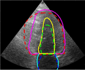
(a) $2$CH-ES: $d_{m}$-endo = 2.5, $d_{m}$-epi = 3.9 , $d_{H}$-endo = 12.6 , $d_{H}$-epi = 13.3 mm.

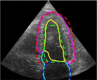
(b) $4$CH-ES: $d_{m}$-endo = 3.0 , $d_{m}$-epi = 2.4 , $d_{H}$-endo = 15.7 , $d_{H}$-epi = 10.1 mm.

Figure 22: Anatomically plausible and inconceivable outliers.

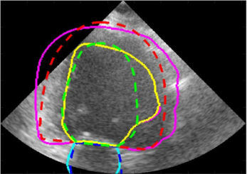
(a) $2$CH-ED: $d_{m}$-endo = 7.3, $d_{m}$-epi = 6.1 , $d_{H}$-endo = 23.2 , $d_{H}$-epi = 16.5 mm.

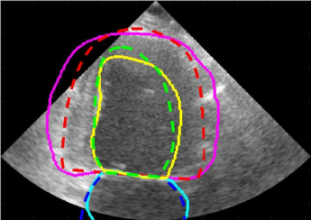
(b) $2$CH-ES: $d_{m}$-endo = 3.8, $d_{m}$-epi = 5.7 , $d_{H}$-endo = 11.1 , $d_{H}$-epi = 12.0 mm.

Figure 23: Outliers that may benefit from temporal coherency on the LV shape.

References

- [1] C. Armstrong, E. P. Ricketts, C. Cox, P. Adler, A. Arynchyn et al., “Quality Control and Reproducibility in M-Mode, Two-Dimensional, and Speckle Tracking Echocardiography Acquisition and Analysis: The CARDIA Study, Year 25 Examination Experience,” Echocardiography, vol. 32, no. 8, pp. 1233–1240, 2015.
- [2] O. Bernard, A. Lalande, C. Zotti, F. Cervenansky, et al., “Deep Learning Techniques for Automatic MRI Cardiac Multi-structures Segmentation and Diagnosis: Is the Problem Solved?” IEEE Transactions on Medical Imaging, in press, 2018.
- [3] O. Bernard, J. G. Bosch, B. Heyde, M. Alessandrini, D. Barbosa, S. Camarasu-Pop, F. Cervenansky, S. Valette, O. Mirea et al., “Standardized Evaluation System for Left Ventricular Segmentation Algorithms in 3D Echocardiography,” IEEE Transactions on Medical Imaging, vol. 35, no. 4, pp. 967–977, 2016.
- [4] D. Barbosa, D. Friboulet, J. D’hooge, and O. Bernard, “Fast tracking of the left ventricle using global anatomical affine optical flow and local recursive block matching,” in Proc. MICCAI Challenge on Echocardiographic Three-Dimensional Ultrasound Segmentation (CETUS), Boston, MIDAS Journal, 2014, pp. 17–24.
- [5] J. Pedrosa, S. Queirós, O. Bernard, J. Engvall, T. Edvardsen, E. Nagel, and J. D’hooge, “Fast and Fully Automatic Left Ventricular Segmentation and Tracking in Echocardiography Using Shape-Based B-Spline Explicit Active Surfaces,” IEEE Transactions on Medical Imaging, vol. 36, no. 11, pp. 2287–2296, 2017.
- [6] J. A. Noble and D. Boukerroui, “Ultrasound image segmentation: a survey,” IEEE Transactions on Medical Imaging, vol. 25, no. 8, pp. 987–1010, 2006.
- [7] G. Carneiro, J. C. Nascimento, and A. Freitas, “The Segmentation of the Left Ventricle of the Heart From Ultrasound Data Using Deep Learning Architectures and Derivative-Based Search Methods,” IEEE Transactions on Image Processing, vol. 21, no. 3, pp. 968–982, 2012.
- [8] K. Y. E. Leung and J. G. Bosch, “Automated border detection in three-dimensional echocardiography: principles and promises,” European Journal of Echocardiography, vol. 11, no. 2, pp. 97–108, 2010.
- [9] C. Wang and O. Smedby, “Model-based left ventricle segmentation in 3d ultrasound using phase image,” in Proc. MICCAI Challenge on Echocardiographic Three-Dimensional Ultrasound Segmentation (CETUS), Boston, MIDAS Journal, 2014, pp. 81–88.
- [10] E. Smistad and F. Lindseth, “Real-time tracking of the left ventricle in 3d ultrasound using kalman filter and mean value coordinates,” in Proc. MICCAI Challenge on Echocardiographic Three-Dimensional Ultrasound Segmentation (CETUS), Boston, MIDAS Journal, 2014, pp. 65–72.
- [11] M. Bernier, P. Jodoin, and A. Lalande, “Automatized evaluation of the left ventricular ejection fraction from echocardiographic images using graph cut,” in Proc. MICCAI Challenge on Echocardiographic Three-Dimensional Ultrasound Segmentation (CETUS), Boston, MIDAS Journal, 2014, pp. 25–32.
- [12] F. Milletari, M. Yigitsoy, N. Navab, and S. Ahmadi, “Left ventricle segmentation in cardiac ultrasound using hough-forests with implicit shape and appearance priors,” in Proc. MICCAI Challenge on Echocardiographic Three-Dimensional Ultrasound Segmentation (CETUS), Boston, MIDAS Journal, 2014, pp. 49–56.
- [13] M. van Stralen, A. Haak, K. Leung, G. van Burken, and J. Bosch, “Segmentation of multi-center 3d left ventricular echocardiograms by active appearance models,” in Proc. MICCAI Challenge on Echocardiographic Three-Dimensional Ultrasound Segmentation (CETUS), Boston, MIDAS Journal, 2014, pp. 73–80.
- [14] O. Oktay, W. Shi, K. Keraudren, J. Caballero, and D. Rueckert, “Learning shape representations for multi-atlas endocardium segmentation in 3D echo images,” in Proc. MICCAI Challenge on Echocardiographic Three-Dimensional Ultrasound Segmentation (CETUS), Boston, MIDAS Journal, 2014, pp. 57–64.
- [15] K. Keraudren, O. Oktay, W. Shi, J. Hajnal, and D. Rueckert, “Endocardial 3d ultrasound segmentation using autocontext random forests,” in Proc. MICCAI Challenge on Echocardiographic Three-Dimensional Ultrasound Segmentation (CETUS), Boston, MIDAS Journal, 2014, pp. 41–48.
- [16] J. Domingos, R. Stebbing, and J. Noble, “Endocardial segmentation using structured random forests in 3D echocardiography,” in Proc. MICCAI Challenge on Echocardiographic Three-Dimensional Ultrasound Segmentation (CETUS), Boston, MIDAS Journal, 2014, pp. 33–40.
- [17] E. Smistad, A. Østvik, B. O. Haugen, and L. Lovstakken, “2D left ventricle segmentation using deep learning,” in 2017 IEEE International Ultrasonics Symposium (IUS), 2017, pp. 1–4.
- [18] O. Ronneberger, P. Fischer, and T. Brox, “U-Net: Convolutional Networks for Biomedical Image Segmentation,” in Proc. MICCAI, 2015, pp. 234–241.
- [19] O. Oktay, E. Ferrante, K. Kamnitsas, M. Heinrich, W. Bai, J. Caballero, S. A. Cook, A. de Marvao, T. Dawes, D. P. O‘Regan, B. Kainz, B. Glocker, and D. Rueckert, “Anatomically Constrained Neural Networks (ACNNs): Application to Cardiac Image Enhancement and Segmentation,” IEEE Transactions on Medical Imaging, vol. 37, no. 2, pp. 384–395, 2018.
- [20] Ö. Çiçek, A. Abdulkadir, S. S. Lienkamp, T. Brox, and O. Ronneberger, “3D U-Net: Learning Dense Volumetric Segmentation from Sparse Annotation,” in Medical Image Computing and Computer-Assisted Intervention – MICCAI 2016. Cham: Springer International Publishing, 2016, pp. 424–432.
- [21] E. D. Folland, A. F. Parisi, P. F. Moynihan, D. R. Jones, C. L. Feldman, and D. E. Tow, “Assessment of left ventricular ejection fraction and volumes by real-time, two-dimensional echocardiography. A comparison of cineangiographic and radionuclide techniques,” Circulation, vol. 60, no. 4, pp. 760–766, 1979.
- [22] R. M. Lang, L. P. Badano, V. Mor-Avi, J. Afilalo et al., “Recommendations for Cardiac Chamber Quantification by Echocardiography in Adults: An Update from the American Society of Echocardiography and the European Association of Cardiovascular Imaging,” Circulation, vol. 28, no. 1, pp. 1–39, 2015.
- [23] G. Litjens, T. Kooi, B. E. Bejnordi, A. A. A. Setio, F. Ciompi, M. Ghafoorian, J. A. van der Laak, B. van Ginneken, and C. I. Sánchez, “A survey on deep learning in medical image analysis,” Med. Image Anal., vol. 42, pp. 60 – 88, 2017.
- [24] A. Newell, K. Yang, and J. Deng, “Stacked hourglass networks for human pose estimation,” in Computer Vision – ECCV 2016, B. Leibe, J. Matas, N. Sebe, and M. Welling, Eds. Cham: Springer International Publishing, 2016, pp. 483–499.
- [25] Z. Zhou, M. Siddiquee, N. Tajbakhsh, and J. Liang, “Unet++: A nested u-net architecture for medical image segmentation,” in in proc. of Deep Learning in Medical Image Analysis and Multimodal Learning for Clinical Decision Support, 2018, pp. 3–11.
- [26] S. Leclerc, T. Grenier, F. Espinosa, and O. Bernard, “A fully automatic and multi-structural segmentation of the left ventricle and the myocardium on highly heterogeneous 2D echocardiographic data,” in IEEE International Ultrasonics Symposium (IUS), 2017.
- [27] P. Dollár and C. L. Zitnick, “Fast Edge Detection Using Structured Forests,” IEEE Transactions on Pattern Analysis and Machine Intelligence, vol. 37, no. 8, pp. 1558–1570, 2015.
- [28] D. Barbosa, T. Dietenbeck, J. Schaerer, J. D’hooge, D. Friboulet, and O. Bernard, “B-Spline Explicit Active Surfaces: An Efficient Framework for Real-Time 3-D Region-Based Segmentation,” IEEE Transactions on Image Processing, vol. 21, no. 1, pp. 241–251, 2012.
- [29] J. Pedrosa, D. Barbosa, B. Heyde, F. Schnell, A. Rösner, P. Claus, and J. D’hooge, “Left Ventricular Myocardial Segmentation in 3-D Ultrasound Recordings: Effect of Different Endocardial and Epicardial Coupling Strategies,” IEEE Transactions on Ultrasonics, Ferroelectrics, and Frequency Control, vol. 64, no. 3, pp. 525–536, March 2017.
- [30] D. Barbosa, T. Dietenbeck, B. Heyde, H. Houle, D. Friboulet, J. D’hooge, and O. Bernard, “Fast and Fully Automatic 3-D Echocardiographic Segmentation Using B-Spline Explicit Active Surfaces: Feasibility Study and Validation in a Clinical Setting,” Ultrasound in Medicine & Biology, vol. 39, no. 1, pp. 89 – 101, 2013.
Supplementary materials for: