Taking rational numbers at random

Abstract

We outline some simple prescriptions to define a distribution on the set $\mathbb{Q}_{0}$ of all the rational numbers in $[0,1]$, and we then explore both a few properties of these distributions, and the possibility of making these rational numbers asymptotically equiprobable in a suitable sense. In particular it will be shown that in the said limit – albeit no uniform distribution can be properly defined on $\mathbb{Q}_{0}$ – the probability allotted to a single $q\in\mathbb{Q}_{0}$ asymptotically vanishes, while that of the subset of $\mathbb{Q}_{0}$ falling in an interval $[a,b]$ goes to $b-a$. We finally give some hints to completely sequencing without repetitions the numbers in $\mathbb{Q}_{0}$ as a prerequisite to the laying down of more distributions on it

Key words: Rational numbers; Discrete distributions; Randomness

1 Introduction

What could the locution taking at random possibly mean? In its most general sense this would indicate that the drawing of an outcome $\omega$ out of a set $\Omega$ is made according to any arbitrary (but legitimate) probability measure assigned on the subsets of $\Omega$, and then that the usual precepts of the probability theory are followed with the result that different probabilities are normally allocated to distinct subsets of $\Omega$. Traditionally however the meaning of the said locution is more circumscribed and stands rather for assuming that there is no reason to think that there are preferred outcomes $\omega\in\Omega$, these being supposed instead to be equally likely. This will be the meaning that we will be interested in all along this paper, or – whether this notion will not be exactly applicable – an asymptotic version of it in some acceptable limiting sense

It is well known indeed that for the sets of real numbers our kind of randomness is enforced either by sheer equiprobability (on the finite sets), or by distribution uniformity (on the bounded, Lebesgue measurable, uncountable sets). On the other hand infinite, countable sets and unbounded, uncountable sets are both excluded from these egalitarian probability attributions because their elements can be made neither equiprobable (with a non vanishing probability), nor uniformly distributed (with a non vanishing probability density). In these occasions it is advisable instead to start with some proper (neither equiprobable, nor uniform) probability distribution, and then to inquire if and how this can be made ever closer – in a suitable, approximate sense – either to an equiprobable or to an uniform one: we will then respectively speak of asymptotic equiprobability and asymptotic uniformity

The focus of our present inquiry, as will be elucidated in the Section 2, are the rational numbers that – even in a bounded interval – constitute an infinite, countable set, with a few relevant, additional peculiarities due to their being also everywhere dense among the real numbers. In the Section 3 we will then supply a procedure to attribute non vanishing probabilities to every rational number $q=\,\!^{n}/_{m}$ in the interval $[0,1]$. The Section 4 is instead devoted to the aftermaths of supposing conditionally equiprobable numerators $n$, and then the Section 5 will show under which hypotheses our distributions can give rise to an asymptotic equiprobability of the rationals in $[0,1]$ such that – without pretending to have a uniform distribution on $\mathbb{Q}_{0}$ – the probability allotted to a single $q\in\mathbb{Q}_{0}$ vanishes in the limit, while that of the subset of $\mathbb{Q}_{0}$ falling in an interval $[a,b]$ goes to $b-a$. Several examples of denominator distributions are elaborated in the Section 6 giving rise to a few closed formulas, and finally in the Section 7 some concluding remarks are added with a glimpse on the open problem of sequencing all the rational numbers in $\mathbb{Q}_{0}$

2 Probability on rational numbers

Rational numbers are famously countable, and hence they can be put in a sequence. Since however they are a dense subset of the real numbers, every rational number is a cluster point, and hence no sequence encompassing all of them can ever converge, not to say be monotone. In any case their countability certainly allows the allotment of discrete distributions with non vanishing probabilities for every rational number: since they are infinite, however, they can never be exactly equiprobable. We will outline in the forthcoming sections a simple procedure to give distributions on the rationals in $[0,1]$, a set that we will shortly denote as $\mathbb{Q}_{0}=\mathbb{Q}\cap[0,1]$, and we will investigate if and how they can be considered asymptotically equiprobable. We will refrain instead for the time being from extending our considerations to the whole of $\mathbb{Q}$ only because in our opinion this – at the present stage of the inquiry – would not add particular insights to our discussion

It is however advisable to assert right away that the distribution of a rv (random variable) $Q$ taking values in $\mathbb{Q}_{0}$ must anyhow be of a discrete type, allotting (possibly non vanishing) probabilities to the individual rational numbers $q\in\mathbb{Q}_{0}$: conceivable continuous set functions – namely with continuous, albeit perhaps not absolutely continuous, cdf (cumulative distribution function) – would turn out to be not countably additive, and hence would not qualify as measures, not to say as probability distributions. Every continuous cdf for $Q$ would indeed entail that at the same time ${\bm{P}}\left\{{Q=q}\right\}=0,\;\forall q\in\mathbb{Q}_{0}$, and ${\bm{P}}\left\{{Q\in\mathbb{Q}_{0}}\right\}=1$, while $\mathbb{Q}_{0}$ apparently is the countable union of the disjoint, negligible sets $\{q\}$: in plain conflict with the countable additivity. This in particular rules out for the numbers in $\mathbb{Q}_{0}$ also the possibility of being in some sense uniformly distributed (an imaginable surrogate of equiprobability suggested by the rationals density): this property would in fact require for $Q$ a cdf of the uniform type

$$F_{Q}(x)={\bm{P}}\left\{{Q\leq x}\right\}=\left\{\begin{array}[]{ll}0&\quad\hbox{$x<0$}\\ x&\quad\hbox{$0\leq x<1$}\\ 1&\quad\hbox{$1\leq x$}\end{array}\right.$$

which is apparently continuous, and would hence attribute probability $0$ to every single $q$, but probability $1$ to $\mathbb{Q}_{0}$

We would like to stress, moreover, that the problem focused on in the present paper is not how to realistically produce – possibly equiprobable – rational numbers at random: this would be performed in a trivial way, for instance, just by taking random, uniformly distributed real numbers, and then by truncating them to a prefixed number $n$ of decimal digits, as always done in practice in every computer simulations of random numbers in $[0,1]$. It is apparent however that in so doing we would shrink $\mathbb{Q}_{0}$ to a finite set of rational numbers (they would be exactly $10^{n}+1$) that could always be made exactly equiprobable, failing instead to allot a non vanishing probability to the remaining, overwhelmingly more numerous, elements of $\mathbb{Q}_{0}$. The aim of our inquiry is instead to find a sensible way to attribute (non vanishing, and possibly not too different from each other) probabilities to every rational number in $\mathbb{Q}_{0}$, their practical simulation being considered here but an eventual side effect of this allocation

Remark that one could be lured to think that a way around the previous snag could consist in drawing again uniformly distributed real numbers, yet truncating the decimal digits to some random number $N$ taking arbitrary, finite but unbounded integer values. Even in this way, however, not every rational number would have a chance to be produced: the said procedure would indeed a priori exclude all the (infinitely many) rational numbers with an infinite, periodic decimal representation, as for instance ${}^{1}/_{3},\,\!^{2}/_{3},\ldots$ and so on. In the light of this preliminary scrutiny the best way to tackle the task of laying down a probability on $\mathbb{Q}_{0}$ seems then to be to exploit the fractional representation $q=\,\!^{n}/_{m}$ of every rational number by attributing some suitable joint distribution to its numerators and denominators

3 Distributions on $\mathbb{Q}_{0}$

Taking advantage of the well known diagram used to prove the countability of the rational numbers, we will consider two dependent rv’s $M$ and $N$ with integer values

$$m=1,2,\ldots\qquad\qquad n=0,1,2,\ldots,m$$

and acting respectively as denominator and numerator of the random rational number $Q=\,^{N}/_{M}\in[0,1]$. As a consequence $Q$ will take the values $q=\,^{n}/_{m}$ arrayed in a triangular scheme as in Table 1.

					$\bm{n}$
$\bm{m}$	$0$	$1$	$2$	$3$	$4$	$5$	$6$	$7$	$8$	$\ldots$
$1$	$0$	$1$
$2$	$0$	${}^{1}/_{2}$	$1$
$3$	$0$	${}^{1}/_{3}$	${}^{2}/_{3}$	$1$
$4$	$0$	${}^{1}/_{4}$	${}^{2}/_{4}$	${}^{3}/_{4}$	$1$
$5$	$0$	${}^{1}/_{5}$	${}^{2}/_{5}$	${}^{3}/_{5}$	${}^{4}/_{5}$	$1$
$6$	$0$	${}^{1}/_{6}$	${}^{2}/_{6}$	${}^{3}/_{6}$	${}^{4}/_{6}$	${}^{5}/_{6}$	$1$
$7$	$0$	${}^{1}/_{7}$	${}^{2}/_{7}$	${}^{3}/_{7}$	${}^{4}/_{7}$	${}^{5}/_{7}$	${}^{6}/_{7}$	$1$
$8$	$0$	${}^{1}/_{8}$	${}^{2}/_{8}$	${}^{3}/_{8}$	${}^{4}/_{8}$	${}^{5}/_{8}$	${}^{6}/_{8}$	${}^{7}/_{8}$	$1$
$\vdots$	$\vdots$									$\ddots$

Table 1: Table of rational numbers $q=\,\!^{n}/_{m}$ with repetitions: many fractions are reducible to canonical forms already present in earlier positions

It is apparent however that in this way every rational number $q$ shows up infinitely many times due to the presence of reducible fractions: for instance – with the usual notation for repeating decimals – we have

$$0.5=\,\!^{1}/_{2}=\,\!^{2}/_{4}=\,\!^{3}/_{6}=\ldots\qquad 0.\overline{3}=\,\!^{1}/_{3}=\,\!^{2}/_{6}=\ldots\qquad 0.75=\,\!^{3}/_{4}=\,\!^{6}/_{8}=\ldots$$

and hence, to avoid repetitions, the rational numbers in $[0,1]$ should rather be listed with blanks as in Table 2. While always possible in principle, however, it would be uneasy to assign probabilities directly to the elements of the said Table 2: there is in fact no simple way to attribute a progressive index to them (what for instance is the $1\,000^{th}$ element?) since the numbers $\nu_{m}$ of the different rationals in every row sharing a common irreducible denominator $m$ constitute a rather irregular sequence, as we will briefly discuss in the Section 7. As a consequence it is advisable to take advantage of the complete Table 1 by introducing a joint distributions of $N$ and $M$

						$\bm{n}$
$\bm{\nu_{m}}$	$\bm{m}$	$0$	$1$	$2$	$3$	$4$	$5$	$6$	$7$	$\ldots$
2	$1$	$0$	$1$
1	$2$		${}^{1}/_{2}$
2	$3$		${}^{1}/_{3}$	${}^{2}/_{3}$
2	$4$		${}^{1}/_{4}$		${}^{3}/_{4}$
4	$5$		${}^{1}/_{5}$	${}^{2}/_{5}$	${}^{3}/_{5}$	${}^{4}/_{5}$
2	$6$		${}^{1}/_{6}$				${}^{5}/_{6}$
6	$7$		${}^{1}/_{7}$	${}^{2}/_{7}$	${}^{3}/_{7}$	${}^{4}/_{7}$	${}^{5}/_{7}$	${}^{6}/_{7}$
4	$8$		${}^{1}/_{8}$		${}^{3}/_{8}$		${}^{5}/_{8}$		${}^{7}/_{8}$
$\vdots$	$\vdots$		$\vdots$							$\ddots$

Table 2: Table of rational numbers $q\doteq\,\!^{n}/_{m}$ without repetitions: only irreducible fractions are represented, along with the number $\nu_{m}$ of the different rationals sharing a common irreducible denominator $m$

$${\bm{P}}\left\{{M=m}\right\}\qquad\qquad\qquad\;m=1,2,\ldots$$

$${\bm{P}}\left\{{N=n\left|M=m\right.}\right\}\qquad\quad\,n=0,1,2,\ldots,m$$

$${\bm{P}}\left\{{N=n,M=m}\right\}={\bm{P}}\left\{{N=n\left|M=m\right.}\right\}\,{\bm{P}}\left\{{M=m}\right\}$$

For a rational number $q$ we will also adopt the notation

$$q\doteq\,\!^{n}/_{m}$$

to indicate that ${}^{n}/_{m}$ is the irreducible representation of $q$, namely that $n$ and $m$ are co-primes: for instance in the previous examples it will be

$$0.5\doteq\,\!^{1}/_{2}\qquad\quad 0.\overline{3}\doteq\,\!^{1}/_{3}\qquad\quad 0.75\doteq\,\!^{3}/_{4}$$

For every rational $q\doteq\,\!^{n}/_{m}$ we will then have the discrete distribution

$${\bm{P}}\left\{{Q=q}\right\} = \sum_{\ell=1}^{\infty}{\bm{P}}\left\{{N=\ell n,M=\ell m}\right\}$$ (1)

$$= \sum_{\ell=1}^{\infty}{\bm{P}}\left\{{N=\ell n\left|M=\ell m\right.}\right\}\,{\bm{P}}\left\{{M=\ell m}\right\}$$

which gives a probability to every rational number $0\leq q\leq 1$. This also allows to define the cdf of $Q$ as (here of course $x\in{\mathbb{R}}$)

$$F_{Q}(x) = {\bm{P}}\left\{{Q\leq x}\right\}={\bm{P}}\left\{{N\leq Mx}\right\}=\sum_{m=1}^{\infty}{\bm{P}}\left\{{N\leq mx\left|M=m\right.}\right\}{\bm{P}}\left\{{M=m}\right\}$$ (2)

$$= \sum_{m=1}^{\infty}F_{N}(mx|M=m){\bm{P}}\left\{{M=m}\right\}$$

and hence also the probability of $Q$ falling in $(a,b]$ for $0\leq a<b\leq 1$ real numbers:

$${\bm{P}}\left\{{a<Q\leq b}\right\} = F_{Q}(b)-F_{Q}(a)$$ (3)

$$= \sum_{m=1}^{\infty}\big{[}F_{N}(mb|M=m)-F_{N}(ma|M=m)\big{]}{\bm{P}}\left\{{M=m}\right\}$$

Notice that the conditional cdf of $N$ can also be given as

$$F_{N}(x|M=m) = {\bm{P}}\left\{{N\leq x\left|M=m\right.}\right\}=\sum_{n=0}^{m}{\bm{P}}\left\{{N=n\left|M=m\right.}\right\}\vartheta(x-n)$$ (4)

$$= \sum_{n=0}^{\lfloor x\rfloor}{\bm{P}}\left\{{N=n\left|M=m\right.}\right\}$$

where

$$\vartheta(x)=\left\{\begin{array}[]{ll}1&\qquad x\geq 0\\ 0&\qquad x<0\end{array}\right.$$

is the Heaviside function, while for every real number $x$, the symbol $\lfloor x\rfloor$ denotes the floor of $x$, namely the greatest integer less than or equal to $x$. As a consequence the equations (2) and (3) also take the form

$$F_{Q}(x)\!\! = \!\!\sum_{m=1}^{\infty}{\bm{P}}\left\{{M=m}\right\}\sum_{n=0}^{\lfloor mx\rfloor}{\bm{P}}\left\{{N=n\left|M=m\right.}\right\}$$ (5)

$${\bm{P}}\left\{{a<Q\leq b}\right\}\!\! = \!\!\sum_{m=1}^{\infty}{\bm{P}}\left\{{M=m}\right\}(1-\delta_{\lfloor ma\rfloor,\lfloor mb\rfloor})\!\!\!\sum_{n=\lfloor ma\rfloor+1}^{\lfloor mb\rfloor}\!\!\!\!{\bm{P}}\left\{{N=n\left|M=m\right.}\right\}$$ (6)

where the Kronecker delta takes into account the fact that when $\lfloor mb\rfloor=\lfloor ma\rfloor$ the term vanishes, so that $\lfloor mb\rfloor\geq\lfloor ma\rfloor+1$. We moreover have for the expectations and the characteristic function

$${\bm{E}}\,\!\left[{Q}\right] = {\bm{E}}\,\!\left[{\,\!{}^{N}/_{M}}\right]={\bm{E}}\,\!\left[{\frac{1}{M}{\bm{E}}\,\!\left[{N|M}\right]}\right]=\sum_{m=1}^{\infty}\frac{{\bm{P}}\left\{{M=m}\right\}}{m}{\bm{E}}\,\!\left[{N|M=m}\right]$$ (7)

$${\bm{E}}\,\!\left[{Q^{2}}\right] = \sum_{m=1}^{\infty}\frac{{\bm{P}}\left\{{M=m}\right\}}{m^{2}}{\bm{E}}\,\!\left[{\left.N^{2}\right|M=m}\right]$$ (8)

$$\varphi_{Q}(u) = {\bm{E}}\,\!\left[{e^{iuN/M}}\right]=\sum_{m=1}^{\infty}{\bm{P}}\left\{{M=m}\right\}\sum_{n=0}^{m}e^{iun/m}{\bm{P}}\left\{{N=n\left|M=m\right.}\right\}$$ (9)

$$= \sum_{m=1}^{\infty}{\bm{P}}\left\{{M=m}\right\}\varphi_{N}\left({}^{u}/_{m}\left|M=m\right.\right)$$

where we also adopted the shorthand notation

$$\varphi_{N}\left(u\left|M=m\right.\right)={\bm{E}}\,\!\left[{e^{iuN}\left|M=m\right.}\right]=\sum_{n=0}^{m}e^{iun}{\bm{P}}\left\{{N=n\left|M=m\right.}\right\}$$

The actual joint distributions of $N$ and $M$ can now be chosen in several ways, and we go on now in the next sections to survey a few particular cases

4 Equiprobable numerators

Let us suppose now for simplicity that for a given denominator $m\geq 1$ the $m+1$ possible values of the numerator $n=0,1,\ldots,m$ are equiprobable in the sense that

$${\bm{P}}\left\{{N=n\left|M=m\right.}\right\}=\frac{1}{m+1}\qquad\quad n=0,1,\ldots,m$$

We then have (see [1] $\bm{0.121}$)

$${\bm{E}}\,\!\left[{N|M=m}\right] = \sum_{n=0}^{m}\frac{n}{m+1}=\frac{1}{m+1}\,\frac{m(m+1)}{2}=\frac{m}{2}$$

$${\bm{E}}\,\!\left[{\left.N^{2}\right|M=m}\right] = \sum_{n=0}^{m}\frac{n^{2}}{m+1}=\frac{1}{m+1}\,\frac{m(m+1)(2m+1)}{6}=\frac{m(2m+1)}{6}$$

and hence from (7) and (8)

$${\bm{E}}\,\!\left[{Q}\right] = \sum_{m=1}^{\infty}\frac{{\bm{P}}\left\{{M=m}\right\}}{m}\,\frac{m}{2}=\frac{1}{2}\sum_{m=1}^{\infty}{\bm{P}}\left\{{M=m}\right\}=\frac{1}{2}$$

$${\bm{E}}\,\!\left[{Q^{2}}\right] = \sum_{m=1}^{\infty}\frac{{\bm{P}}\left\{{M=m}\right\}}{m^{2}}{\bm{E}}\,\!\left[{N^{2}|M=m}\right]=\sum_{m=1}^{\infty}\frac{2m+1}{6m}{\bm{P}}\left\{{M=m}\right\}$$

$$= \frac{1}{3}\sum_{m=1}^{\infty}{\bm{P}}\left\{{M=m}\right\}+\frac{1}{6}\sum_{m=1}^{\infty}\frac{{\bm{P}}\left\{{M=m}\right\}}{m}=\frac{1}{3}+\frac{1}{6}{\bm{E}}\,\!\left[{\frac{1}{M}}\right]$$

$${\bm{V}}\left[{Q}\right] = {\bm{E}}\,\!\left[{Q^{2}}\right]-{\bm{E}}\,\!\left[{Q}\right]^{2}=\frac{1}{12}+\frac{1}{6}{\bm{E}}\,\!\left[{\frac{1}{M}}\right]$$

As for the distribution, with $n,m$ co-primes and $0\leq n\leq m$, from (1) we have

$${\bm{P}}\left\{{Q=q}\right\}=\sum_{\ell=1}^{\infty}\frac{{\bm{P}}\left\{{M=\ell m}\right\}}{\ell m+1}\qquad\quad q\doteq\,\!^{n}/_{m}$$ (10)

which is apparently independent from $n$ and is contingent only on the value of the irreducible denominator $m$. The characteristic function (9) moreover is

$$\varphi_{N}\left(u\left|M=m\right.\right)=\frac{1}{m+1}\sum_{n=0}^{m}e^{iun}\qquad\quad\varphi_{Q}(u)=\sum_{m=1}^{\infty}\frac{{\bm{P}}\left\{{M=m}\right\}}{m+1}\sum_{n=0}^{m}e^{iun/m}$$

while for the cdf (5) we have from (4)

$$F_{N}\left(mx\left|M=m\right.\right) = \frac{1}{m+1}\sum_{n=0}^{m}\vartheta\left(mx-n\right)=\left\{\begin{array}[]{ll}0&\quad\hbox{$x<0$}\\ \frac{\lfloor mx\rfloor+1}{m+1}&\quad\hbox{$0\leq x<1$}\\ 1&\quad\hbox{$1\leq x$}\end{array}\right.$$ (14)

$$F_{Q}(x) = \sum_{m=1}^{\infty}\frac{{\bm{P}}\left\{{M=m}\right\}}{m+1}\sum_{n=0}^{m}\vartheta\left(mx-n\right)$$ (18)

$$= \left\{\begin{array}[]{ll}0&\quad\hbox{$x<0$}\\ \sum_{m\geq 1}{\bm{P}}\left\{{M=m}\right\}\frac{\lfloor mx\rfloor+1}{m+1}&\quad\hbox{$0\leq x<1$}\\ 1&\quad\hbox{$1\leq x$}\end{array}\right.$$

and the probability (6) with $0\leq a<b\leq 1$ becomes

$${\bm{P}}\left\{{a<Q\leq b}\right\}=\sum_{m=1}^{\infty}{\bm{P}}\left\{{M=m}\right\}\frac{\lfloor mb\rfloor-\lfloor ma\rfloor}{m+1}$$ (19)

It is apparent then that – but for the value of the expectation ${\bm{E}}\,\!\left[{Q}\right]=\,\!^{1}/_{2}$ – all these quantities depend on the choice of the denominator distribution. That notwithstanding we will show in the next section that, under reasonable conditions on the denominators $M$, the distribution of $Q$ can in fact be made as near as we want to – but not exactly coincident with – a uniform distribution in $[0,1]$: a behavior that we dubbed asymptotic equiprobability

5 Asymptotic equiprobability

For the equiprobable numerators introduced in the previous section, and by denoting for short as $p_{m}={\bm{P}}\left\{{M=m}\right\}$ the distribution of $M$, and as $s=\sup_{m}p_{m}$ the supremum of all its values, let us take now a sequence of denominators $\{M_{k}\}_{k\geq 1}$ with distributions $\{p_{m}(k)\}_{k\geq 1}$, and with $s_{k}$ vanishing for $k\to\infty$ in such a way that

$$\lim_{k}\,s_{k}\ln k=0$$ (20)

In other words we consider a sequence of distributions that are increasingly (and uniformly) flattened toward zero, so that the denominators too are increasingly equiprobable. Ready examples of these sequences with $k=1,2,\ldots$ are for instance that of the finite equiprobable distributions

$$p_{m}(k)=\left\{\begin{array}[]{ll}{}^{1}/_{k}&\hbox{$m=1,2,\ldots,k$}\\ 0&\hbox{$m>k$}\end{array}\right.$$

where apparently $s_{k}=\,\!^{1}/_{k}\buildrel k\over{\longrightarrow}0\,$; that of the geometric distributions

$$p_{m}(k)=w_{k}(1-w_{k})^{m-1}\quad\qquad m=1,2,\ldots$$

with infinitesimal $w_{k}$ so that $s_{k}=w_{k}\buildrel k\over{\longrightarrow}0\,$; and finally that of the Poisson distributions

$$p_{m}(k)=e^{-\lambda_{k}}\frac{\lambda_{k}^{m-1}}{(m-1)!}\quad\qquad m=1,2,\ldots$$

with divergent $\lambda_{k}$, where again the modal values are infinitesimal: we know indeed that a Poisson distribution attains its maximum in $\lfloor\lambda_{k}\rfloor+1$, so that for $\lambda_{k}\buildrel k\over{\longrightarrow}+\infty$ its modal value $s_{k}$ essentially behaves as (see [1] $\bm{8.327.1}$)

$$s_{k}=e^{-\lambda_{k}}\frac{\lambda_{k}^{\lambda_{k}-1}}{\Gamma(\lambda_{k})}=\frac{1}{\sqrt{2\pi\lambda_{k}}\big{(}1+{O}(\lambda_{k}^{-1})\big{)}}\buildrel k\over{\longrightarrow}0$$

Lemma 5.1.

Within the previous notations and conditions we have

$$\mu_{k}={\bm{E}}\,\!\left[{\,\!{}^{1}/_{M_{k}}}\right]=\sum_{m=1}^{\infty}\frac{p_{m}(k)}{m}\buildrel k\over{\longrightarrow}0$$ (21)

Proof:  The positive series defining $\mu_{k}$ is certainly convergent because

$$\mu_{k}=\sum_{m=1}^{\infty}\frac{p_{m}(k)}{m}<\sum_{m=1}^{\infty}p_{m}(k)=1$$

and hence we can always write

$$\mu_{k}=\sum_{m=1}^{\infty}\frac{p_{m}(k)}{m}=\sum_{m=1}^{k}\frac{p_{m}(k)}{m}+R_{k}$$

where

$$R_{k}=\sum_{m=k+1}^{\infty}\frac{p_{m}(k)}{m}\buildrel k\over{\longrightarrow}0$$

is an infinitesimal remainder. Remark that now $k$ plays both the roles of index of the distribution sequence, and of series cut-off. On the other hand, under our stated conditions

$$\sum_{m=1}^{k}\frac{p_{m}(k)}{m}<s_{k}\sum_{m=1}^{k}\frac{1}{m}=s_{k}H_{k}$$

where $H_{k}$ denotes the $k^{th}$ harmonic number, namely the sum of the reciprocal integers up to ${}^{1}/_{k}$: it is well known ([1] $\bm{0.131}$) that for $k\to\infty$ the $H_{k}$ grow as $\ln k$, so that from (20) we have $s_{k}H_{k}\buildrel k\over{\longrightarrow}0$, and finally $\mu_{k}=s_{k}H_{k}+R_{k}\buildrel k\over{\longrightarrow}0$ $\blacksquare$

Proposition 5.2.

If $Q=\,\!^{N}/_{M}$ and $F_{Q}(x)$ is its cdf, then, within the notation and conditions outlined above, we have

$$\lim_{k}{\bm{P}}\left\{{Q=q}\right\}=0\qquad\qquad\lim_{k}{\bm{P}}\left\{{a<Q\leq b}\right\}=b-a$$ (22)

$$\qquad\qquad\quad\lim_{k}F_{Q}(x)=\left\{\begin{array}[]{ll}0&\quad\hbox{$x<0$}\\ x&\quad\hbox{$0\leq x<1$}\\ 1&\quad\hbox{$1\leq x$}\end{array}\right.$$ (26)

Proof:  Since our series have positive terms the first result in (22) follows from (10) and (21) because, with $q\doteq\,\!^{n}/_{j}$

$${\bm{P}}\left\{{Q=q}\right\}=\sum_{\ell=1}^{\infty}\frac{p_{\ell j}(k)}{\ell j+1}<\sum_{m=1}^{\infty}\frac{p_{m}(k)}{m+1}<\sum_{m=1}^{\infty}\frac{p_{m}(k)}{m}=\mu_{k}\buildrel k\over{\longrightarrow}0$$

As for the second result in (22), since for every real number $x$ it is $x-1\leq\lfloor x\rfloor\leq x$, for every $k=1,2,\ldots$, and $0\leq a<b\leq 1$, we have from (19)

$$\sum_{m=1}^{\infty}p_{m}(k)\frac{m(b-a)-1}{m+1}\leq\,{\bm{P}}\left\{{a<Q\leq b}\right\}\,\leq\sum_{m=1}^{\infty}p_{m}(k)\frac{m(b-a)+1}{m+1}$$

namely

$$b-a+(a-b-1)\sum_{m=1}^{\infty}\frac{p_{m}(k)}{m+1}\leq\,{\bm{P}}\left\{{a<Q\leq b}\right\}\,\leq b-a+(a-b+1)\sum_{m=1}^{\infty}\frac{p_{m}(k)}{m+1}$$

so that, since $a-b-1\leq 0$ and $a-b+1\geq 0$, it is

$$b-a+(a-b-1)\mu_{k}\leq\,{\bm{P}}\left\{{a<Q\leq b}\right\}\,\leq b-a+(a-b+1)\mu_{k}$$

The second result (22) follows then from (21). In a similar way we finally find for (26) that

$$\sum_{m=1}^{\infty}p_{m}(k)\frac{mx}{m+1}\leq F_{Q}(x)\leq\sum_{m=1}^{\infty}p_{m}(k)\frac{mx+1}{m+1}\qquad\quad 0\leq x\leq 1$$

namely

$$x-x\sum_{m=1}^{\infty}\frac{p_{m}(k)}{m+1}\leq F_{Q}(x)\leq x+(1-x)\sum_{m=1}^{\infty}\frac{p_{m}(k)}{m+1}$$

and hence

$$x-x\,\mu_{k}<F_{Q}(x)<x+(1-x)\mu_{k}$$

so that the result again follows from (21) $\blacksquare$

From this proposition we see that in the limit $k\to\infty$, while the probability of every single rational number rightly vanishes, the probability of these numbers lumped together in intervals does not: a behavior highly reminiscent of what happens to continuously distributed real rv’s. For the reasons presented in the Section 2, however, the previous result by no means imply that we can implement a uniform limit distribution on $\mathbb{Q}_{0}$ (as we said, there is not such a thing), but it rather suggests that our random rational numbers $Q$ – at least for denominators $m$ distributed in a fairly flat way, and numerators $n$ conditionally equiprobable between $0$ and $m$ – asymptotically behave as uniformly distributed in $[0,1]$, and hence they quite reasonably correspond to our intuitive idea of taking rational numbers at random. In this perspective remark also that, under our conditions, we have for the variance

$${\bm{V}}\left[{Q}\right]=\frac{1}{12}+\frac{1}{6}\,{\bm{E}}\,\!\left[{\frac{1}{M}}\right]=\frac{1}{12}+\frac{\mu_{k}}{6}\buildrel k\over{\longrightarrow}\frac{1}{12}$$

again in agreement with an approximate uniform distribution in $[0,1]$

6 Denominator distributions

6.1 Geometric denominators

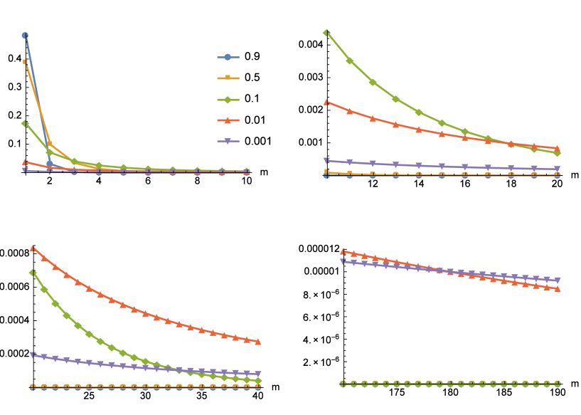
Figure 1: Probabilities attributed to rational numbers as a function of the irreducible, geometrically distributed denominators $m$, and for decreasing ($0.9,0.5,0.1,0.01,0.001$) values of $w$: by choosing different $m$ intervals, the pictures show how these probabilities level down to infinitesimal equiprobability for $w\to 0$

A few closed formulas about the rv $Q$ are available for particular denominator distributions: let us suppose for instance that the denominator $M$ be geometrically distributed as

$${\bm{P}}\left\{{M=m}\right\}=w\,(1-w)^{m-1}\qquad\quad w>0,\qquad m=1,2,\ldots$$

In this case we first find

$${\bm{E}}\,\!\left[{M}\right]=\frac{1}{w}\quad\qquad{\bm{E}}\,\!\left[{\frac{1}{M}}\right]=\sum_{m=1}^{\infty}\frac{w(1-w)^{m-1}}{m}=\frac{w}{1-w}\sum_{m=1}^{\infty}\frac{(1-w)^{m}}{m}=-\frac{w\,\ln w}{1-w}$$

and hence

$${\bm{V}}\left[{Q}\right]=\frac{1}{12}-\frac{w\,\ln w}{6(1-w)}$$

while for the cdf we do not go beyond its formal definition

$$F_{Q}(x)=\left\{\begin{array}[]{ll}0&\quad\hbox{$x<0$}\\ \sum_{m\geq 1}w\,(1-w)^{m-1}\frac{\lfloor mx\rfloor+1}{m+1}&\quad\hbox{$0\leq x<1$}\\ 1&\quad\hbox{$1\leq x$}\end{array}\right.$$

As for the $Q$ distribution instead, taking $q\doteq\,\!^{n}/_{m}$, we find with $j=\ell-1$ the analytic expression

$${\bm{P}}\left\{{Q=q}\right\} = \sum_{\ell=1}^{\infty}\frac{w(1-w)^{\ell m-1}}{\ell m+1}=w(1-w)^{m-1}\sum_{\ell=1}^{\infty}\frac{(1-w)^{m(\ell-1)}}{\ell m+1}$$ (27)

$$= w(1-w)^{m-1}\sum_{j=0}^{\infty}\frac{(1-w)^{mj}}{m(j+1)+1}$$

$$= \frac{w(1-w)^{m-1}}{m+1}\,_{2}F_{1}\left(1,1+\,\!^{1}/_{m}\,;2+\,\!^{1}/_{m}\,;(1-w)^{m}\right)$$

where ${}_{2}F_{1}(a,b;c;z)$ is a hypergeometric function [1] that gauges the deviation of ${\bm{P}}\left\{{Q=q}\right\}$ from the corresponding joint probability of $N,M$

$${\bm{P}}\left\{{N=n,M=m}\right\}=\frac{w(1-w)^{m-1}}{m+1}$$

This formula allows a graphic representation of ${\bm{P}}\left\{{Q=q}\right\}$ as a function of the irreducible denominators $m$ displayed in the Figure 1 where it is apparent how the initial ($m=1$) ordering of the probabilities (increasing with the $w$ values going from $w=0.001$ to $w=0.9$) becomes totally overturned for $m$ large enough. Remark that each value of the probability (27) should be understood as attributed to every rational number with the same $m$ as irreducible denominator, for instance (see Table 2): for $m=1$ we get the probability of $q\doteq 0$ and $1$; for $m=2$ the probability of $q\doteq\,\!^{1}/_{2}$ alone; for $m=3$ that of $q\doteq\,\!^{1}/_{3}\,,^{2}/_{3}\,$; for $m=4$ that of $q\doteq\,\!^{1}/_{4}\,,^{3}/_{4}\,;\,\ldots\,$ and so on. This allows, in particular, to steer clear of an easy misunderstanding: it must be noticed indeed that, while apparently

$$\sum_{m=1}^{\infty}\sum_{n=0}^{m}{\bm{P}}\left\{{N=n,M=m}\right\}=\sum_{m=1}^{\infty}\sum_{n=0}^{m}\frac{w(1-w)^{m-1}}{m+1}=\sum_{m=1}^{\infty}w(1-w)^{m-1}=1$$

we find instead

$$\sum_{m=1}^{\infty}\sum_{n=0}^{m}\frac{w(1-w)^{m-1}}{m+1}\,_{2}F_{1}\left(1,1+\,\!^{1}/_{m}\,;2+\,\!^{1}/_{m}\,;(1-w)^{m}\right)<1$$

as can be seen from the fact that for $0<w<1$

$${}_{2}F_{1}\left(1,1+\,\!^{1}/_{m}\,;2+\,\!^{1}/_{m}\,;(1-w)^{m}\right)\;\left\{\begin{array}[]{ll}=1&\qquad\hbox{$m=1$}\\ <1&\qquad\hbox{$m=2,3,\ldots$}\end{array}\right.$$

This however is not in contradiction with the mandatory requirement that

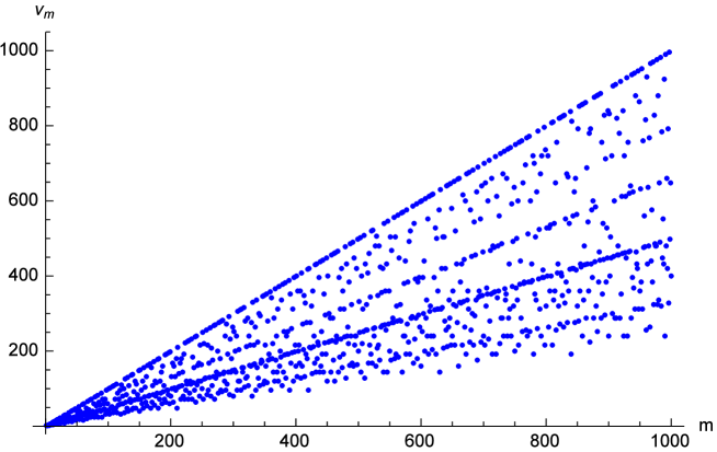
Figure 2: Numerosity $\nu_{m}$ of the different rational numbers $q\doteq\,\!^{n}/_{m}$ sharing a common, irreducible denominator $m$

$$\sum_{q\in\mathbb{Q}_{0}}{\bm{P}}\left\{{Q=q}\right\}=1$$ (28)

precisely because – as previously remarked – the probability associated to an $m$ must be attributed to several different rational numbers $q$: if $\nu_{m}$ is the number of rationals $q$ that have $m$ as its irreducible denominator, then we should rather pay attention to ascertain the normalization in the form

$$\sum_{q\in\mathbb{Q}_{0}}{\bm{P}}\left\{{Q=q}\right\} = \sum_{m=1}^{\infty}\sum_{n=0}^{m}\nu_{m}\,\frac{w(1-w)^{m-1}}{m+1}\,_{2}F_{1}\left(1,1+\,\!^{1}/_{m}\,;2+\,\!^{1}/_{m}\,;(1-w)^{m}\right)$$

$$= \sum_{m=1}^{\infty}\nu_{m}\,w(1-w)^{m-1}\,_{2}F_{1}\left(1,1+\,\!^{1}/_{m}\,;2+\,\!^{1}/_{m}\,;(1-w)^{m}\right)=1$$

Yet this result – that we can consider as secured by construction and definition – is not easy to check by direct calculation because a closed form for the sequence $\nu_{m}$ is not readily available: its behavior is indeed rather irregular, albeit on average steadily growing, as can be seen from an empirical plot of its first values displayed in the Figure 2. We postpone to the Section 7 a few additional remarks about this point showing in particular how the previous normalization condition can instead be used to sequentially calculate the values of $\nu_{m}$

6.2 Poisson and equiprobable denominators

When on the other hand the denominators are distributed according to other (albeit simple) laws we unfortunately no longer find elementary closed forms for ${\bm{P}}\left\{{Q=q}\right\}$. If the for instance $M$ is Poisson distributed as

$${\bm{P}}\left\{{M=m}\right\}=e^{-\lambda}\,\frac{\lambda^{m-1}}{(m-1)!}\qquad\quad\lambda>0,\qquad m=1,2,\ldots$$

we find ${\bm{E}}\,\!\left[{M}\right]=1+\lambda$ and

$${\bm{E}}\,\!\left[{\frac{1}{M}}\right]=\sum_{m=1}^{\infty}\frac{e^{-\lambda}}{m}\,\frac{\lambda^{m-1}}{(m-1)!}=\frac{e^{-\lambda}}{\lambda}\sum_{m=1}^{\infty}\frac{\lambda^{m}}{m!}=\frac{e^{-\lambda}}{\lambda}\left(\sum_{m=0}^{\infty}\frac{\lambda^{m}}{m!}-1\right)=\frac{1-e^{-\lambda}}{\lambda}$$

while for the variance we have

$${\bm{V}}\left[{Q}\right]=\frac{1}{12}+\frac{1-e^{-\lambda}}{6\lambda}$$

but the cdf is

$$F_{Q}(x)=\left\{\begin{array}[]{ll}0&\quad\hbox{$x<0$}\\ e^{-\lambda}\,\sum_{m\geq 1}\frac{\lambda^{m-1}}{(m-1)!}\,\frac{\lfloor mx\rfloor+1}{m+1}&\quad\hbox{$0\leq x<1$}\\ 1&\quad\hbox{$1\leq x$}\end{array}\right.$$

and for the distribution, taking $q\doteq\,\!^{n}/_{m}$, we find

$${\bm{P}}\left\{{Q=q}\right\}=\sum_{\ell=1}^{\infty}\frac{e^{-\lambda}}{\ell m+1}\,\frac{\lambda^{\ell m-1}}{(\ell m-1)!}$$

with no closed expression readily available

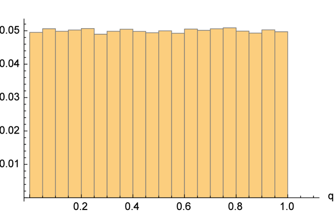
Figure 3: Typical histogram of the relative frequencies of a sample of $10^{5}$ random rationals generated following the procedure described in the Section 6.2: here the maximum value of the equiprobable denominators is chosen to be $k=10^{5}$

Consider instead denominators $M$ taking only a finite number $k=1,2,\ldots$ of equiprobable values $m$:

$${\bm{P}}\left\{{M=m}\right\}=\left\{\begin{array}[]{ll}{}^{1}/_{k}&\hbox{$m=1,2,\ldots,k$}\\ 0&\hbox{$m>k$}\end{array}\right.$$

We then have

$${\bm{E}}\,\!\left[{M}\right]=\frac{k+1}{2}\qquad\qquad{\bm{E}}\,\!\left[{\frac{1}{M}}\right]=\frac{1}{k}\sum_{m=1}^{k}\frac{1}{m}=\frac{H_{k}}{k}$$

and hence

$${\bm{V}}\left[{Q}\right]=\frac{1}{12}+\frac{H_{k}}{6k}$$

while for the cdf it is

$$F_{Q}(x)=\frac{1}{k}\sum_{m=1}^{k}\frac{\lfloor mx\rfloor+1}{m+1}$$

and the discrete distribution probabilities are

$${\bm{P}}\left\{{Q=q}\right\}=\frac{1}{k}\sum_{\ell=1}^{\lfloor\,\!^{k}/_{m}\rfloor}\frac{1}{\ell m+1}\qquad\quad q\doteq\,\!^{n}/_{m}$$

where, since $m\leq k$, it is always $\lfloor\,\!^{k}/_{m}\rfloor=1,2,\ldots$.

Even in this case we have then no closed formulas to show, but since the sums involved are now always finite this seems to hint to a simple – but essentially trivial – procedure to simulate an asymptotically equiprobable sample of rational numbers in $[0,1]$: choose first a large enough number $k$, then sample a random integer $m$ among the equiprobable numbers $1,2,\ldots,k$, and finally a random integer $n$ among the equiprobable numbers $0,1,\ldots,m$ and put $q=\,\!^{n}/_{m}$. By repeating this procedure a number of times large enough we get a sample almost uniformly distributed in $[0,1]$ as shown in Figure 3. The drawback of this procedure, however, as already remarked in the Section 2, is that not every number in $\mathbb{Q}_{0}$ would have the chance of being drawn because only a finite number among them would actually be taken into account. This large but finite set of numbers could also be made, in principle, exactly equiprobable, but the infinitely many remaining rational numbers would instead be totally excluded with strictly zero probability

7 Sequencing rational numbers

Other examples of distributions on the rational numbers in $[0,1]$ are of course possible: for instance, with $0<p<1$ and for a given denominator $m=1,2,\ldots$, it is possible to suppose that the numerators are binomially – instead of equiprobably – distributed as

$${\bm{P}}\left\{{N=n\left|M=m\right.}\right\}={m\choose n}p_{(}1-p)^{m-n}\qquad\quad n=0,1,\ldots,m$$

By choosing then a suitable distribution for the denominator $M$ we can define the global distribution of $Q=\,\!^{N}/_{M}$. However, rather than indulging in displaying these further examples, we would like to conclude this paper with a few remarks about a particular residual open problem

								$\bm{n}$
$\bm{\sigma_{m}}$	$\bm{\nu_{m}}$	$\bm{m}$	$0$	$1$	$2$	$3$	$4$	$5$	$6$	$7$	$8$	$9$	$10$
$1$	$2$	$1$	$0$	$1$
${}^{1}/_{2}$	$1$	$2$		${}^{1}/_{2}$
$1$	$2$	$3$		${}^{1}/_{3}$	${}^{2}/_{3}$
$1$	$2$	$4$		${}^{1}/_{4}$		${}^{3}/_{4}$
$2$	$4$	$5$		${}^{1}/_{5}$	${}^{2}/_{5}$	${}^{3}/_{5}$	${}^{4}/_{5}$
$1$	$2$	$6$		${}^{1}/_{6}$				${}^{5}/_{6}$
$3$	$6$	$7$		${}^{1}/_{7}$	${}^{2}/_{7}$	${}^{3}/_{7}$	${}^{4}/_{7}$	${}^{5}/_{7}$	${}^{6}/_{7}$
$2$	$4$	$8$		${}^{1}/_{8}$		${}^{3}/_{8}$		${}^{5}/_{8}$		${}^{7}/_{8}$
$3$	$6$	$9$		${}^{1}/_{9}$	${}^{2}/_{9}$		${}^{4}/_{9}$	${}^{5}/_{9}$		${}^{7}/_{9}$	${}^{8}/_{9}$
$2$	$4$	$10$		${}^{1}/_{10}$		${}^{3}/_{10}$				${}^{7}/_{10}$		${}^{9}/_{10}$
$5$	$10$	$11$		${}^{1}/_{11}$	${}^{2}/_{11}$	${}^{3}/_{11}$	${}^{4}/_{11}$	${}^{5}/_{11}$	${}^{6}/_{11}$	${}^{7}/_{11}$	${}^{8}/_{11}$	${}^{9}/_{11}$	${}^{10}/_{11}$
$\vdots$	$\vdots$	$\vdots$		$\vdots$									$\vdots$

Table 3: Table of rational numbers $q\doteq\,\!^{n}/_{m}$ without repetitions, along with the progressive number $\nu_{m}$ of the different rationals sharing a common irreducible denominator $m$, and their sums $\sigma_{m}$

We said from the beginning that since $\mathbb{Q}_{0}$ is countable its elements $0\leq q\leq 1$ can certainly be arranged in a sequence. If on the other hand we can manage to have in this sequence all the rational numbers without repetitions, this would greatly facilitate the task of giving a distribution on $\mathbb{Q}_{0}$. In order however to put in a sequence without repetitions $q_{k}$ all these rational numbers in $[0,1]$ – as listed for instance in the triangular, infinite Table 3 – we should at least be able to find regularities in their arrangement allowing to say with relative easy both what is the rational number $q$ associated to an arbitrary given index $k$, and viceversa what is the place (index $k$) of an arbitrary given rational number $q$. But this quest is baffled by the rather irregular running of the entries in the said triangular table where, for instance, even the occurrence among the denominators $m$ of the prime numbers (the only ones identifying rows with no blanks beyond the extremes) is famously not immediately predictable. It is apparent however that the possibility of effectively sequencing all the numbers in $\mathbb{Q}_{0}$ is primarily contingent on some knowledge about $\nu_{m}$, namely the number of the non-blank entries in the $m^{th}$ row of Table 3

Without pretending to treat thoroughly this topic, we will just confine ourselves to a few remarks about some simple properties of the numbers $\nu_{m}$ (the number of rational numbers present in a row of Table 3 sharing a common irreducible denominator $m$) and $\sigma_{m}$ (the sum of the said rational numbers). First of all it should be said that the normalization condition (28) can be used to find a procedure to progressively calculate the values of $\nu_{m}$. For instance, as stated in the Section 6.1, when denominators are geometrically distributed and numerators are conditionally equiprobable, the distribution of $Q$ is (27) and the normalization (28) must be enforced by taking into account the number $\nu_{m}$ of the equiprobable numbers sharing the same irreducible denominator. It is easy to see then that, by taking $z=1-w$ in (27), the normalization condition (28) becomes

$$\sum_{q\in\mathbb{Q}_{0}}{\bm{P}}\left\{{Q=q}\right\}=\frac{1-z}{z^{2}}\sum_{m=1}^{\infty}\nu_{m}\sum_{\ell=1}^{\infty}\frac{z^{m\ell+1}}{m\ell+1}=1$$

namely with a power expansion

$$\sum_{m=1}^{\infty}\nu_{m}\sum_{\ell=1}^{\infty}\frac{z^{m\ell+1}}{m\ell+1}=\frac{z^{2}}{1-z}=\sum_{j=0}^{\infty}z^{j+2}$$ (29)

This relation can be used to find the values of $\nu_{m}$ by equating the coefficients of the identical powers of $z$: by explicitly writing indeed the first terms of (29) we find

$$\nu_{1}\left(\frac{z^{2}}{2}+\frac{z^{3}}{3}+\frac{z^{4}}{4}+\frac{z^{5}}{5}+\ldots\right)+\nu_{2}\left(\frac{z^{3}}{3}+\frac{z^{5}}{5}+\frac{z^{7}}{7}+\frac{z^{9}}{9}+\ldots\right)$$

$$\qquad\qquad+\nu_{3}\left(\frac{z^{4}}{4}+\frac{z^{7}}{7}+\frac{z^{10}}{10}+\frac{z^{13}}{13}+\ldots\right)+\nu_{4}\left(\frac{z^{5}}{5}+\frac{z^{9}}{9}+\frac{z^{13}}{13}+\frac{z^{17}}{17}+\ldots\right)+\ldots$$

$$\qquad=z^{2}+z^{3}+z^{4}+z^{5}+\ldots$$

and hence we progressively have

$${}^{\nu_{1}}/_{2}=1 \nu_{1}=2$$

$${}^{\nu_{1}}/_{3}+\,\!^{\nu_{2}}/_{3}=1 \nu_{2}=1$$

$${}^{\nu_{1}}/_{4}+\,\!^{\nu_{3}}/_{4}=1 \nu_{3}=2$$

$${}^{\nu_{1}}/_{5}+\,\!^{\nu_{2}}/_{5}+\,\!^{\nu_{4}}/_{5}=1 \nu_{4}=2$$

$$\ldots \ldots$$

and so on, in apparent agreement with the corresponding entries of the Table 3. It must be added that this procedure can not be contingent on the specific distribution of $Q$ because $\nu_{m}$ is always the same sequence and the normalization condition (28) must hold for every legitimate distribution

We will finally list a few elementary properties of $\nu_{m}$ and $\sigma_{m}$ that can be helpful for every future advance: here $m=1,2,\ldots$ are the denominators, $n=0,1,\ldots,m$ the numerators and we call them accepted when ${}^{n}/_{m}$ appears in the Table 3, namely if it is an irreducible fraction:

1. $\bm{\nu_{m}\leq m-1}$ for $\bm{m\geq 2}$: in our table $n=0$ and $n=m$ are accepted only for $m=1$ so that in every row with $m\geq 2$ the first and last number are always missing; then apparently $\nu_{m}=(m+1)-2=m-1$; in particular $\bm{\nu_{m}=m-1}$ only for $\bm{m}$ prime number

2. for $\bm{m\geq 3}$, if $\bm{n=k\geq 1}$ is accepted, then also $\bm{n=m-k\leq m-1}$ is accepted because, if ${}^{k}/_{m}$ is irreducible, then also ${}^{(m-k)}/_{m}=1-\,\!^{k}/_{m}$ is irreducible, namely the accepted values always show up in pairs; in particular, since $n=1$ is always accepted, then also $n=m-1$ is always accepted and hence $\bm{\nu_{m}\geq 2}$ for $\bm{m\geq 3}$ (the two numbers coincide for $m=2$, so that $\nu_{2}=1$)

3. $\bm{\nu_{m}}$ always is an even number for $\bm{m\geq 3}$ because according to the point 2 the accepted numerators $n$ always show up in pairs; moreover if $\bm{m\geq 3}$ is even, then $\bm{n=\,\!^{m}/_{2}}$ is not accepted because for $m=2\ell$ (and $\ell\geq 2$) the numerator would be $n=\,\!^{m}/_{2}=\ell$, and ${}^{n}/_{m}=\,\!^{\ell}/_{2\ell}$ would be a reducible fraction

4. for $\bm{m\geq 3}$ the sum of an accepted pair always is $\bm{1}$ because we are adding ${}^{k}/_{m}$ and ${}^{(m-k)}/_{m}=1-\,\!^{k}/_{m}$; as a consequence the sum of the irreducible fractions sharing a common denominator $\bm{m}$ is $\bm{\sigma_{m}=\,\!^{\nu_{m}}/_{2}}$ because there are $\,{}^{\nu_{m}}/_{2}$ accepted pairs; looking moreover at the Table 3 we see that this last result holds also for $m=1$ ($\nu_{1}=2,\,\sigma_{1}=1$) and $m=2$ ($\nu_{2}=1,\,\sigma_{2}=\,\!^{1}/_{2}$)

References

- [1] I.S. Gradshteyn and I.M. Ryzhik, Table of Integrals, Series and Products (Academic Press, Burlington 2007)