Large-scale Environmental Data Science with ExaGeoStatR

Abstract

Parallel computing in exact Gaussian process calculations becomes necessary for avoiding computational and memory restrictions associated with large-scale environmental data science applications. The exact evaluation of the Gaussian log-likelihood function requires $O(n^{2})$ storage and $O(n^{3})$ operations where $n$ is the number of geographical locations. Thus, exactly computing the log-likelihood function with a large number of locations requires exploiting the power of existing parallel computing hardware systems, such as shared-memory, possibly equipped with GPUs, and distributed-memory systems, to solve this exact computational complexity. In this paper, we present ExaGeoStatR, a package for exascale Geostatistics in R that supports a parallel computation of the exact maximum likelihood function on a wide variety of parallel architectures. Furthermore, the package allows scaling existing Gaussian process methods to a large spatial/temporal domain. Prohibitive exact solutions for large geostatistical problems become possible with ExaGeoStatR. Parallelization in ExaGeoStatR depends on breaking down the numerical linear algebra operations in the log-likelihood function into a set of tasks and rendering them for a task-based programming model. The package can be used directly through the R environment on parallel systems without the user needing any C, CUDA, or MPI knowledge. Currently, ExaGeoStatR supports several maximum likelihood computation variants such as exact, Diagonal Super Tile (DST) and Tile Low-Rank (TLR) approximations, and Mixed-Precision (MP). ExaGeoStatR also provides a tool to simulate large-scale synthetic datasets. These datasets can help assess different implementations of the maximum log-likelihood approximation methods. Herein, we show the implementation details of ExaGeoStatR, analyze its performance on various parallel architectures, and assess its accuracy using synthetic datasets with up to 250K observations. The experimental analysis covers the exact computation of ExaGeoStatR to demonstrate the parallel capabilities of the package. We provide a hands-on tutorial to analyze a sea surface temperature real dataset. The performance evaluation involves comparisons with the popular packages GeoR, fields, and bigGP for exact Gaussian likelihood evaluation. The approximation methods in ExaGeoStatR are not considered in this paper since they were analyzed in previous studies.

I Introduction

Massive data require a delicate analysis to extract meaningful information from their complex structure. With the availability of large data volumes coming from different sources, an objective of data science is to combine a set of principles and techniques from data mining, machine learning, and statistics to support a better understanding of the given data. Like other sciences, environmental science has been very much impacted by the field of data science. Indeed, a vast pool of techniques has been developed to understand spatial and spatio-temporal data coming from intelligent sensors or satellite images. However, new challenges have arisen with today’s data sizes that require a unique treatment paradigm.

Environmental applications deal with measurements regularly or irregularly located across a geographical region. Gaussian processes (GPs), or Gaussian Random Fields (GRFs), are among the most useful tools in applications for fitting spatial datasets. For the last two decades, GPs have been used extensively to model spatial data and are able to cover a wide range of spatial data with different specifications [Gelfand and Schliep, 2016]. Spatial data can also be described as random effects, hence they can often be modeled with a Gaussian distribution. Therefore, the dependencies in spatial data can be described through a Gaussian process.

GRFs also serve as building blocks for numerous non-Gaussian models in spatial statistics such as trans-Gaussian random fields, mixture GRFs and skewed GRFs. For example, Xu and Genton [2017] introduced the Tukey $g$-and-$h$ random field which modifies the GRF by a flexible form of variable transformation; Andrews and Mallows [1974], West [1987], and Rue and Held [2005] considered the scale-mixture of Gaussian distributions and GRFs; and Allard and Naveau [2007] and Azzalini [2005] proposed many skewed GRFs and their variations. However, likelihood-based inference methods for GP models are computationally expensive for large-scale spatial datasets. It is crucial to provide fast computational tools to fit a GP model to large-scale spatial datasets often available in many real-world applications.

Specifically, suppose $Z({\mathbf{s}})$ is a stationary GRF with mean function $m({\mathbf{s}})$ and covariance function $C({\mathbf{s}},{\mathbf{s}}^{\prime})$, and we observe data on a domain $D\subset\mathbb{R}^{d}$ at $n$ locations, $\mathbf{s}_{1},\ldots,\mathbf{s}_{n}$. Then, the random vector $\{Z(\mathbf{s}_{1}),\ldots,Z(\mathbf{s}_{n})\}^{\top}$ is assumed to follow a multivariate Gaussian distribution:

$$\forall\{\mathbf{s}_{1},\ldots,\mathbf{s}_{n}\}\subset D,\quad\{Z(\mathbf{s}_{1}),\ldots,Z(\mathbf{s}_{n})\}^{\top}\sim{\cal N}_{n}(\boldsymbol{\mu},{\mathbf{\Sigma}}),$$ (1)

where $\boldsymbol{\mu}=\{m(\mathbf{s}_{1}),\ldots,m(\mathbf{s}_{n})\}^{\top}$ and ${\mathbf{\Sigma}}$ are the mean vector and the covariance matrix of the $n$-dimensional multivariate normal distribution. Given $\boldsymbol{\mu}$ and ${\mathbf{\Sigma}}$, the (Gaussian) likelihood of observing $\mathbf{z}=\{z(\mathbf{s}_{1}),\ldots,z(\mathbf{s}_{n})\}^{\top}$ at the $n$ locations is

$$L(\boldsymbol{\mu},\mathbf{\Sigma})=\frac{1}{(2\pi)^{n/2}|{\mathbf{\Sigma}}|^{1/2}}\exp\left\{-\frac{1}{2}(\mathbf{z}-\boldsymbol{\mu})^{\top}{\mathbf{\Sigma}}^{-1}(\mathbf{z}-\boldsymbol{\mu})\right\}.$$ (2)

The $(i,j)$-th element of $\mathbf{\Sigma}$ is $\Sigma_{ij}=C(\mathbf{s}_{i},\mathbf{s}_{j})$, where the covariance function $C(\mathbf{s}_{i},\mathbf{s}_{j})$ is assumed to have a parametric form with unknown vector of parameters $\boldsymbol{\theta}$. Various classes of covariance functions can be found in e.g. Cressie [2015]. For simplicity, in this work, we assume the mean vector $\boldsymbol{\mu}$ to be zero to focus on estimating the covariance parameters. We choose the most popular isotropic Matérn covariance kernel, which is specified as,

$$\Sigma_{ij}=C(\|\mathbf{s}_{i}-\mathbf{s}_{j}\|)=\frac{\sigma^{2}}{2^{\nu-1}\Gamma(\nu)}\left(\frac{\|\mathbf{s}_{i}-\mathbf{s}_{j}\|}{\beta}\right)^{\nu}\mathcal{K}_{\nu}\left(\frac{\|\mathbf{s}_{i}-\mathbf{s}_{j}\|}{\beta}\right),$$ (3)

where $\|\mathbf{s}_{i}-\mathbf{s}_{j}\|$ is the Euclidean distance between $\mathbf{s}_{i}$ and $\mathbf{s}_{j}$, $\Gamma(\cdot)$ is the gamma function, $\mathcal{K}_{\nu}(\cdot)$ is the modified Bessel function of the second kind of order $\nu$, and $\sigma^{2}$, $\beta>0$, and $\nu>0$ are the key parameters of the covariance function controlling the variance, spatial range, and smoothness, respectively. The Matérn covariance kernel is highly flexible and includes the exponential ($\nu=1/2$) and Gaussian ($\nu=\infty$) kernels as special cases. The variance, spatial range, and smoothness parameters, $\sigma^{2}$, $\beta$, and $\nu$ determine the properties of the GRF.

The typical inference for GRFs includes parameter estimation, stochastic simulation, and kriging (spatial prediction). Among these tasks, parameter estimation, or model fitting, is the most time-consuming. Once the parameters are estimated, one can easily simulate multiple realizations of the GRF or obtain predictions at new locations. To obtain the maximum likelihood estimator (MLE), we need to optimize the likelihood function in Equation (2) over $\boldsymbol{\theta}=(\sigma^{2},\beta,\nu)^{\top}$. However, the likelihood for a given $\boldsymbol{\theta}$ requires computing the inverse ($\mathbf{\Sigma(\boldsymbol{\theta})}^{-1}$) and the determinant ($|\mathbf{\Sigma(\boldsymbol{\theta})}|$) of the covariance matrix $\mathbf{\Sigma}(\boldsymbol{\theta})$, and performing the triangular linear solve ($\mathbf{\Sigma(\boldsymbol{\theta})}^{-1}\mathbf{Z}$). The most time-consuming operation to compute the likelihood function is the Cholesky factorization for $\mathbf{\Sigma}(\boldsymbol{\theta})$, which requires $O(n^{3})$ operations and $O(n^{2})$ memory. This factorization is required to compute the inverse and the determinant of $\mathbf{\Sigma}(\boldsymbol{\theta})$. Due to the likelihood estimation complexity, the standard methods and traditional algorithms for GRFs are computationally infeasible for large datasets.

On the other hand, technological advances in sensor networks along with the investments in data monitoring, collection, resource management provide massive open-access spatial datasets [Finley et al., 2015]. The unprecedented data availability and the challenging computational complexity call for novel methods, algorithms, and software packages to deal with modern “Big Data” problems in spatial statistics.

A broad literature focuses on developing efficient methodologies by approximating the covariance function in the GP model, so that the resulting covariance matrix is easier to compute. Sun et al. [2012], Bradley et al. [2016], and Liu et al. [2020] systematically reviewed these methods. Some popular approximation methods are covariance tapering [Furrer et al., 2006, Kaufman et al., 2008], discrete process convolutions [Higdon, 2002, Lemos and Sansó, 2009], fixed rank kriging [Cressie and Johannesson, 2008], lattice kriging [Nychka et al., 2015], and predictive processes [Banerjee et al., 2008, Finley et al., 2009]. Meanwhile, some studies proposed to approximate the Gaussian likelihood function using conditional distributions [Vecchia, 1988, Katzfuss and Guinness, 2021] or composite likelihoods [Varin et al., 2011, Eidsvik et al., 2014], and some seek for equivalent representation of GPs using spectral density [Fuentes, 2007] and stochastic partial differential equations [Lindgren et al., 2011].

A recent direction of this research aims at developing parallel algorithms [Paciorek et al., 2015, Katzfuss and Hammerling, 2017, Datta et al., 2016, Guhaniyogi and Banerjee, 2018] and using modern computational architectures, such as multicore systems, GPUs, and supercomputers, in order to avoid insufficient approximation of the GP [Simpson et al., 2012, Stein, 2014]. Aggregating computing power through High-Performance Computing (HPC) becomes an important tool in scaling existing software in different disciplines to handle the exponential growth of datasets generated in these fields [Vetter, 2013]. However, the literature lacks a well-developed HPC software that practitioners can use to support their applications with HPC capabilities. Although most studies provide reproducible source codes, they are difficult to extend to new applications, especially when the algorithms require certain hardware setups. R [Ihaka and Gentleman, 1996] is the most popular software in statistics, applied analytics, and interactive exploration of data by far. As a high-level language, however, R is relatively weak for high-performance computing compared to lower-level languages, such as C, C++, and Fortran. Scaling statistical software and bridging high-performance computing with the R language can be performed using two different strategies. One strategy has been followed by the pbdR [Ostrouchov et al., 2012] project, Programming with Big Data in R, which transfers the HPC libraries to the R environment by providing a high-level R interface to a set of HPC libraries such as MPI, ScaLAPACK, ZeroMQ, to name a few. However, one drawback of this strategy is that the R developer should have enough background in HPC to be able to use the provided interfaces to scale his/her code. Another strategy that we adopt in this paper is to implement the statistical functions using an HPC-friendly language such as C. Then it is easier to directly wrap the C functions into R functions. In this case, these functions can directly be used inside the R environment without the need to understand the underlying HPC architectures or the development environment.

This paper presents ExaGeoStatR, a high-performance package in R for large-scale environmental data science and geostatistical applications that depends on a unified C-based software called ExaGeoStat [Abdulah et al., 2018a]. ExaGeoStat is able to fit Gaussian process models and provide spatial predictions and simulations for geostatistics applications in large-scale domains. ExaGeoStat provides both exact and approximate computations for large-scale spatial datasets. Besides the exact method, the software also supports three approximation methods: Diagonal Super Tile (DST), Tile Low-Rank (TLR), and Mixed-Precision (MP) computations. This study highlights the capabilities of the ExaGeoStatR exact computations since it can be considered a benchmark for the performance of other computation methods. Moreover, the evaluation of the DST and the TLR approximations has already been covered in Abdulah et al. [2018a, b, 2019], Hong et al. [2021], Abdulah et al. [2022b]. The software also includes a synthetic dataset generator for generating large spatial datasets with the exact prespecified covariance function. Such large datasets can be used to perform broader scientific experiments related to large-scale computational geostatistics applications. Besides its ability to deal with different hardware architectures such as multicore systems, GPUs, and distributed systems, ExaGeoStatR utilizes the underlying hardware architectures to its full extent. Existing assessments on ExaGeoStat show the ability of the software to handle up to 3.4 million spatial locations on manycore systems with exact calculations [Abdulah et al., 2022b].

Existing R packages for fitting GRFs include GeoR [Ribeiro Jr and Diggle, 2016], fields [Nychka et al., 2017], spBayes [Finley et al., 2007a, 2015], RandomFields [Schlather et al., 2019, 2015a], INLA [Rue et al., 2009, Martins et al., 2013], bigGP [Paciorek et al., 2015]. These packages feature different degrees of flexibility as well as computational capacity. The spBayes package fits GP models in the context of Bayesian or hierarchical modeling based on MCMC. The RandomFields package implements the Cholesky factorization method, the circulant embedding method [Dietrich and Newsam, 1996], and an extended version of Matheron’s turning bands method [Matheron, 1973] for the maximum likelihood estimation of GRFs. The INLA package uses an integrated nested Laplace approximation to tackle additive models with a latent GRF, which outperforms the MCMC method. The bigGP package utilizes distributed memory systems through RMPI [Gropp et al., 1999] to implement the estimation, prediction, and simulation of GRFs. The packages GeoR and fields both estimate the GRF covariance structures designed for spatial statistics while GeoR provides more flexibilities, such as estimating the mean structure and the variable transformation parameters. Among these popular packages, only the bigGP package, according to our knowledge, focuses on distributed computing, which is essential for solving problems in data-rich environments in exact mode. The bigGP package was built using the RMPI and OpenMP libraries to facilitate GP calculations on manycore systems. The bigGP package relies on block-based algorithms to perform the underlying linear algebra operations required to perform the GP calculations. Compared to the bigGP package, ExaGeoStatR provide better performance since it depends on the state-of-the-art parallel linear algebra operations through applying tile-based algorithms to perform the required linear solvers. Table I provides a summary of some of the existing packages for fitting GRFs. The comparison includes common features for each package and if it supports parallel execution or not.

Our package ExaGeoStatR, at the current stage, performs data generation, parameter estimation, and spatial prediction for the univariate GRF with mean zero and a Matérn covariance structure, which is a fundamental model in spatial statistics. We feature breakthroughs in the optimization routine for the maximum likelihood estimation and the utilization of heterogeneous computational units. Specifically, we build on the optimization library NLopt [Johnson, 2014] and provide a unified Application Programming Interface (API) for multicore systems, GPUs, clusters, and supercomputers. The package also supports using the great circle distance on the sphere in constructing the covariance matrix. These parallelization features largely reduce the time-per-iteration in computing exact maximum likelihood estimations compared with existing packages and make GRFs even with $10^{6}$ locations estimable on hardware accessible to most institutions.

The remainder of this paper is organized as follows. Section II states the basics of ExaGeoStatR, and the package components for keen readers. Section III compares the estimation accuracy and time of ExaGeoStatR with two aforementioned exact computation packages, i.e., GeoR and fields, with simulated data. It demonstrates the efficiency that can be gained when the ExaGeoStatR package utilizes powerful architectures including GPUs and distributed memory systems. Section IV is a tutorial to fit a Gaussian random field to a sea surface temperature dataset with more than ten thousand spatial locations per day and perform kriging with the estimated parameter values. Section V concludes with the contributions of the ExaGeoStatR package. In the Appendix, we provide a user guide for installing the ExaGeoStatR package on different hardware environments.

II Software Overview

II-A ExaGeoStat Outline

ExaGeoStat is a C-based software that targets environmental applications through a high-performance parallel implementation of the Maximum Likelihood Estimation (MLE) operation that is widely used for geospatial statistics [Abdulah et al., 2018a]. This software provides a novel solution to deal with the scaling limitation impact of the MLE operation by exploiting the computational power of emerging hardware architectures. ExaGeoStat permits exploring the MLE computational limits using state-of-the-art high-performance dense linear algebra libraries by leveraging a single source code to run on various cutting-edge parallel architectures with the aide of runtime systems software. The “separation of concerns” philosophy adopted by ExaGeoStat from the beginning permits improving the software from different perspectives by allowing fast linear solvers and porting the code to different hardware architectures.

ExaGeoStat is developed to solve the MLE problem for a given set of data observed at $n$ geographical locations on a large scale and to provide a prediction solution for unobserved values at new locations. The software also allows for exact synthetic data generations with a given covariance function, which can be used to test and compare different approximation methods. To sum up, ExaGeoStat includes three primary tools: large-scale synthetic data generator, the Gaussian maximum likelihood estimator, and the geospatial predictor.

In ExaGeoStat, the MLE operation is implemented in four different ways: Fully-Dense (Exact), Diagonal Super Tile (DST) [Abdulah et al., 2018a], Tile Low-Rank (TLR) [Abdulah et al., 2018b], and mixed-precision [Abdulah et al., 2019, 2022b]. The four different implementations rely on state-of-the-art parallel algebraic computations by exploiting advances in algorithmic solutions and manycore computer architectures. The parallel implementation consists in dividing the given covariance matrix into a set of small tiles where a single processing unit can process a single tile at a time. The main difference between different implementations is the structure of the underlying covariance matrix. In dense computation, matrix tiles are represented in fully double-precision format as shown by Figure 1 (a). The provided solution is exact but with the cost of more computing power and storage space. The DST implementation depends on annihilating some of the off-diagonal tiles because their contributions and qualitative impact on the overall statistical problem may be limited while depending on diagonal tiles, which should have a stronger influence on the underlying model. Choosing the number of tiles to be ignored is up to the user who should expect losing some accuracy with more zero tiles. Figure 1 (b) depicts the covariance matrix in the case of DST representation where two-diagonal tiles are represented in dense format while all the other tiles are set to zero. The TLR implementation depends on representing the tiles in low-rank format. Currently, ExaGeoStat supports the Singular Value Decomposition (SVD) technique to compress the off-diagonal tiles in low-rank while other compression methods exist in the literature. The TLR computation depends on the TLR linear algebra operations that can provide fast computation with appropriate accuracy. In Figure 1 (c), the TLR approximation method is used where the $k$ most significant singular values/vectors are captured for each off-diagonal tile to maintain the overall fidelity of the numerical model depending on the application-specific accuracy. Finally, the mixed-precision implementation is inspired by the DST approximation technique. Instead of ignoring some off-diagonal tiles and setting their elements as zero, ExaGeoStat represents their elements in lower-precision, i.e., single or half. In this case, we can speed up the computation compared to the fully-dense implementation but with higher accuracy than the DST approximation. Figures 1 (d) depicts the mixed-precision covariance matrix structure supported by ExaGeoStat.

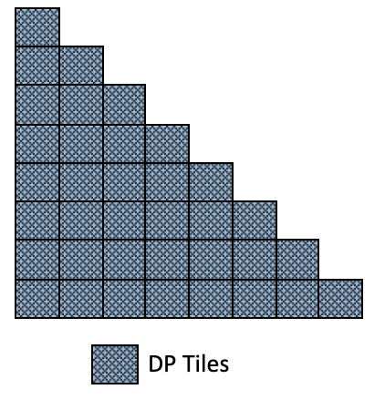
(a) Fully dense (Exact)

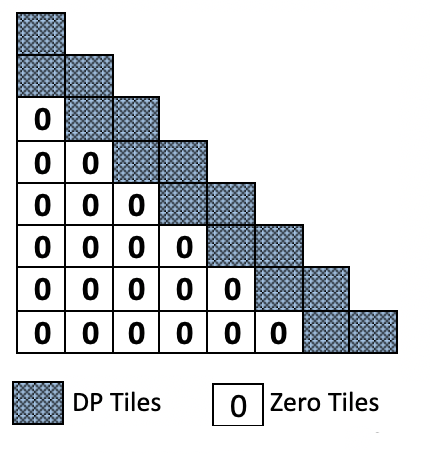
(b) Diag. Super-Tile (DST)

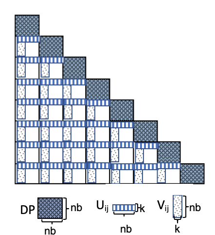
(c) Tile Low-Rank (TLR)

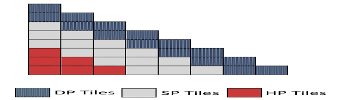
(d) Mixed-Precision (MP)

Figure 1: ExaGeoStat supports various computation methods. The tile is a subset of the matrix with size $ts\times ts$. Here $ts$ should be tuned for performance on parallel systems. DP refers to double-precision (64-bit) tile, SP refers to single-precision (32-bit) tile, and HP refers to half-precision (16-bit) tile.

II-B The ExaGeoStat Infrastructure

To provide the different computational variants shown above, ExaGeoStat internally relies on three parallel linear algebra libraries to construct the basic linear algebra operations for the MLE computation. Exact, DST, and mixed-precision approximation computations rely on the Chameleon library, a high-performance numerical library that provides high-performance dense linear solvers [cha, 2022] or the DPLASMA library, dense linear algebra algorithms on massively parallel architectures [Bosilca et al., 2011]. The TLR approximation computation depends on the HiCMA library, a hierarchical linear algebra library on manycore architectures, that provides parallel approximation solvers [Abdulah et al., 2022a]. The HiCMA is associated with the STARS-H library, a high-performance $\mathcal{H}$-matrix generator library on large-scale systems, which provides test cases for the HiCMA library [sta, 2022]. Both Chameleon and HiCMA libraries provide linear algebra operations through a set of sequential task-based algorithms.

For hardware portability, ExaGeoStat features the StarPU [Augonnet et al., 2011] and PaRSEC [Bosilca et al., 2013] dynamic runtime systems as backends. The runtime system proposes a kind of abstraction to improve the user’s productivity and creativity. For example, Chameleon and HiCMA provide sequential task-based linear algebra operations through a sequential task flow (STF) programming model. StarPU is able to execute the set of given sequential tasks in parallel with given hints of the data dependencies (e.g., read, write, and read-write). The main advantage of using runtime systems that rely on task-based implementations is becoming oblivious to the targeted hardware architecture. Multiple implementations of the same tasks are generated for: CPU, CUDA, OpenCL, OpenMP, and MPI, to name a few. To achieve the highest performance, the runtime system decides which implementation will achieve the highest performance at runtime. For the first execution, the runtime system generates a set of cost models that determine the best hardware for optimal performance during the given tasks. This set of cost models may be saved for future executions.

The top layer of ExaGeoStat is the optimization toolbox. ExaGeoStat relies on an open-source C/C++ nonlinear optimization toolbox, NLopt [Johnson, 2014], to perform the MLE optimization operation. Among 20 global and local optimization algorithms supported by the NLopt library, we selected the Bound Optimization BY Quadratic Approximation (BOBYQA) algorithm to be our optimization algorithm. BOBYQA performs well with our target nonlinear problem with a global maximum point. BOBYQA is a numeric, global, derivative-free, and bound-constrained optimization algorithm. It generates a new computed point on each iteration by solving a trust-region subproblem subject to given constraints. In ExaGeoStat, only upper and lower bound constraints are used. Though BOBYQA does not require evaluating the derivatives of the cost function, it iteratively employs an updated quadratic model of the objective, so there is an implicit assumption of smoothness.

In summary, ExaGeoStat relies on a set of software that expands the software portability capabilities. Figure 2 shows the ExaGeoStat infrastructure with four main layers: the BOBYQA algorithm from the NLopt library for optimization purpose; the log-likelihood estimation upper-level operation; the Chameleon/HiCMA/DPLASMA libraries, which provide exact (the focus of this study) and approximate solvers for the linear algebra operations using task-based parallel algorithms; and the StarPU/PaRSEC dynamic runtime systems, which translate the software for execution on the appropriate underlying hardware. Table II summarizes the complete list of software dependencies. An optimized BLAS library should be available based on the hardware architecture, e.g., Intel MKL for CPU and OpenBLAS for GPU. The hwloc library is used to abstract the underlying hardware topology to the runtime system. In contrast, the GSL library provides a vast set of numerical functions that are needed by some of the covariance functions. For instance, the Bessel and gamma functions for the Matérn covariance function.

Figure 2: ExaGeoStat infrastructure.

II-C ExaGeoStatR Package

To facilitate the use of large-scale executions in the R environment, we present a package in R, i.e., ExaGeoStatR , on top of our ExaGeoStat software that provides high-performance geospatial statistics functions in R. This package in R should help disseminate our software to a large computational and spatial statistics community. To the best of our knowledge, most of the existing R solutions for the MLE problem are sequential and restricted to limited data sizes. A few of them depend on running on multiple cores within the same shared memory system by enabling OpenMP support. ExaGeoStatR targets all the existing parallel hardware architectures, including GPUs and distributed memory systems, with a high-level abstraction of the underlying hardware architecture for the user. Table III gives an overview of current ExaGeoStatR functions with a description of their main operations. We provide an ExaGeoStatR installation tutorial in the Appendix.

III Simulation Studies

In this section, we provide a set of examples with associated code to better understand the ExaGeoStatR package. The examples possess three goals: 1) provide step-by-step instructions of using ExaGeoStatR on multiple different tasks; 2) assess the performance and accuracy of the proposed exact computation compared to existing R packages; and 3) assess the performance of the ExaGeoStatR package using different hardware architectures. All the upcoming experiments rely on the Chameleon linear algebra library and StarPU runtime system when executing the ExaGeoStatR functions.

III-A Performance Evaluation of ExaGeoStatR

The performance of ExaGeoStatR is evaluated on various systems: the experiments in Examples 1 and 2 below are implemented on a Ubuntu 16.04.5 LTS workstation with a dual-socket 8-core Intel Sandy Bridge Intel Xeon E5-2650 without any GPU acceleration; Example 3 is assessed on a dual-socket 14-core Intel Broadwell Intel Xeon CPU E5-2680 v3 running at 2.40 GHz and equipped with 8 NVIDIA K80s (2 GPUs per board), and Example 4 is tested on KAUST’s Cray XC40 supercomputer system, Shaheen II, with 6174 nodes, each node is dual-socket 16-core Intel Haswell processor running at 2.30 GHz and 128 GB of DDR4 memory, and Example 5 is tested on KAUST Ibex cluster with up to 16 nodes. Two popular R packages, GeoR [Ribeiro Jr and Diggle, 2016] and fields [Nychka et al., 2017], are selected as our references for exact computations.

Since ExaGeoStatR works with multiple cores and different hardware architectures, users need to initialize their preferred settings using the exageostat_init function. When users want to change or terminate the current hardware allocation, the exageostat_finalize function is required:

⬇

> library("exageostatr")

> hardware = list (ncores = 2, ngpus = 0, ts = 320, pgrid = 1, qgrid = 1)

> exageostat_init(hardware)

> exageostat_finalize()

The hardware = list() specifies the required hardware to execute the code. Here, ncores and ngpus are the numbers of CPU cores and GPU accelerators to deploy, ts denotes the tile size used for parallelized matrix operations, pgrid and qgrid are the cluster topology parameters in case of distributed memory system execution.

III-B Performance Optimization Options

In general, the performance of the ExaGeoStatR package on shared memory, GPUs, and distributed memory systems can be optimized by explicitly using StarPU optimization environment variables. For example, the STARPU_SCHED environment variable is used to select appropriate parallel tasks scheduling policies provided by StarPU, such as random, eager, and stealing. It determines how to distribute individual tasks to different processing units. The user needs to try various schedulers to satisfy the best performance on the target hardware. Other examples of environment variables are STARPU_LIMIT_MAX_SUBMITTED_TASKS and STARPU_LIMIT_MIN_SUBMITTED_TASKS which control the number of submitted tasks and enable cache buffer reuse in main memory.

III-C Example 1: Data Generation

ExaGeoStatR offers two functions to generate realizations from Gaussian random fields with zero mean and Matérn covariance function shown in Equation (3). The simulate_data_exact function generates a GRF at a set of irregularly spaced random locations. Five inputs need to be given. The $kernel$ input accepts one of seven covariance functions: univariate Gaussian stationary Matérn - space (ugsm-s), bivariate Gaussian stationary flexible Matérn - space (bgsfm-s), bivariate Gaussian stationary parsimonious Matérn - space (bgspm-s), trivariate Gaussian stationary parsimonious Matérn - space (tgspm-s), univariate Gaussian stationary Matérn - space-time (ugsm-st), and bivariate Gaussian stationary Matérn - space-time (bgsm-st). Table IV summarizes the current covariance functions supported by ExaGeoStatR.

The $theta$ input is a vector of the initial model parameters used to generate the simulated target geospatial dataset. The $theta$ vector length depends on the chosen $kernel$. The dmetric input accepts two values: euclidean for Euclidean distance or great_circle for great circle distance in case of spherical data [Veness, 2010]. The $n$ input accepts the number of geospatial locations of the generated data in the unit square as mentioned in  Abdulah et al. [2018a]. The code below gives a simple example of generating a realization from a univariate Gaussian stationary random field at 1600 random locations using the simulate_data_exact function:

⬇

> hardware = list(ncores = 4, ngpus = 0, ts = 320, pgrid = 1, qgrid = 1)

> exageostat_init(hardware)

> data.exageo.irreg = simulate_data_exact(kernel = "ugsm-s", theta= c(1, 0.1, 0.5),

dmetric = "euclidean",n = 1600, seed = 0)

> exageostat_finalize()

The code starts with defining the hardware resources which will be used to run the example. The second line initiates a new ExaGeoStatR instance. The third line simulates synthetic data using a given covariance function with a given parameter vector. Finally, the last line closes the active ExaGeoStatR instance. The results are stored as a list, data=list{x,y,z}, where x and y are coordinates, and z stores the simulated realizations. Here, x and y are generated from a uniform distribution on $[0,1]$. Therefore, the generated locations are irregular on $[0,1]\times[0,1]$ with simulate_data_exact function. To generate data on a regular grid, outside the range of $[0,1]\times[0,1]$, or at specific locations, one can use the simulate_obs_exact function by providing the coordinates x and y. The following code shows an example of generating a GRF on a $[0,2]\times[0,2]$ spatial grid with 1600 locations:

⬇

> hardware = list(ncores = 2, ngpus = 0, ts = 320, pgrid = 1, qgrid = 1)

> exageostat_init(hardware)

> xy = expand.grid((1 : 40) / 20,(1 : 40) / 20)

> x = xy[,1]

> y = xy[,2]

> data.exageo.reg = simulate_obs_exact(x = x, y = y, kernel = "ugsm-s",

theta= c(1, 0.1, 0.5), dmetric = "euclidean")

> exageostat_finalize()

Line 5 in the code simulates synthetic data on given 2d locations using a predefined covariance function and a given parameter vector. In Figure 3, some examples of data simulated using the ExaGeoStatR package at $1600$ locations in the unit square using the univariate Matérn stationary covariance function. The data was generated using $seed=1$.

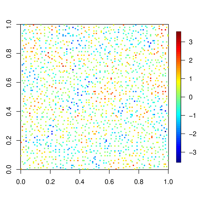
(a) (1, 0.03, 0.5)

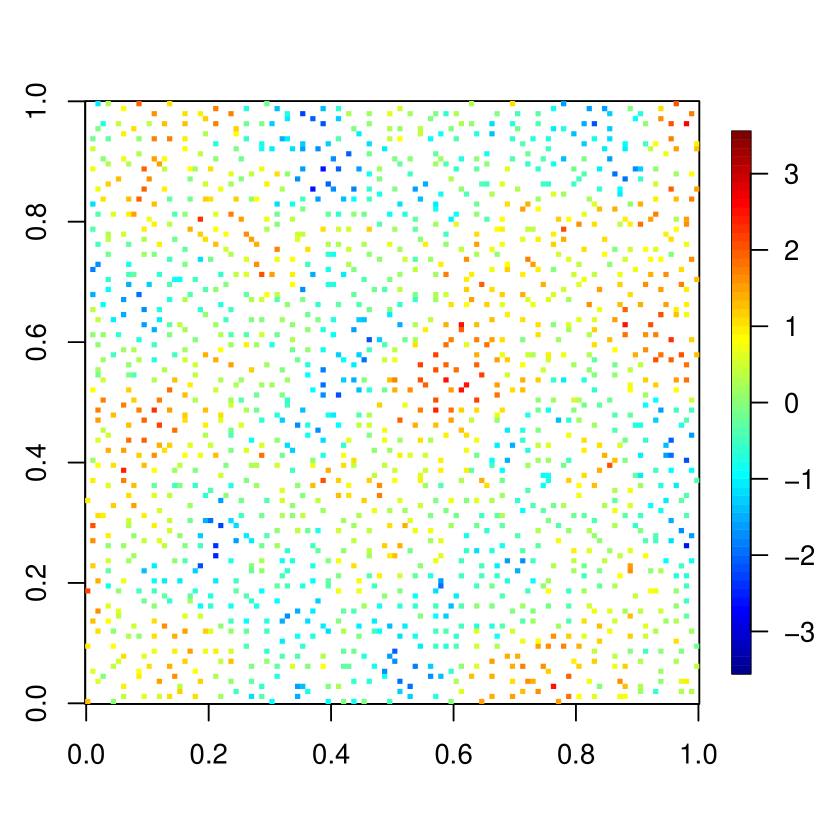
(b) (1, 0.1, 0.5)

(c) (1, 0.3, 0.5)

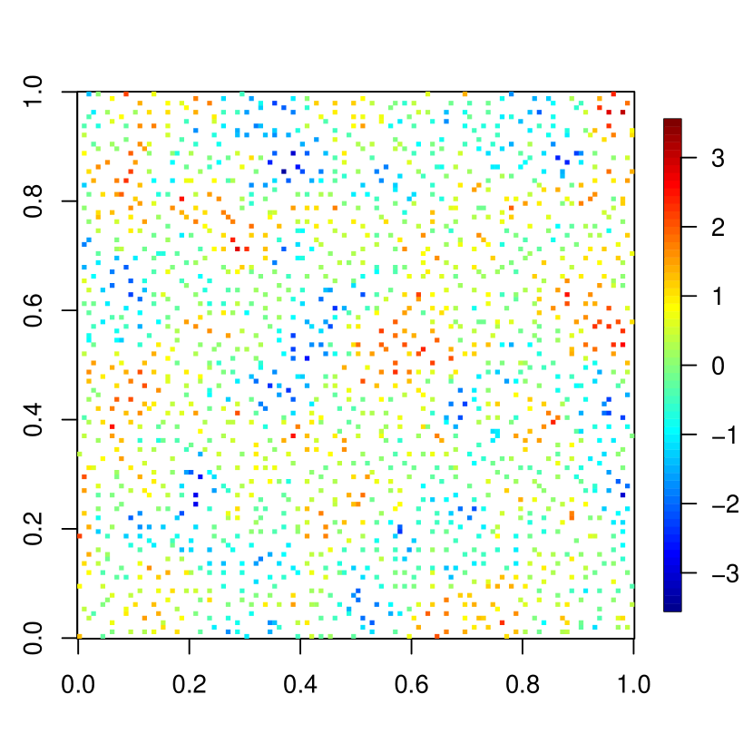
(d) (1, 0.03, 1)

(e) (1, 0.1, 1)

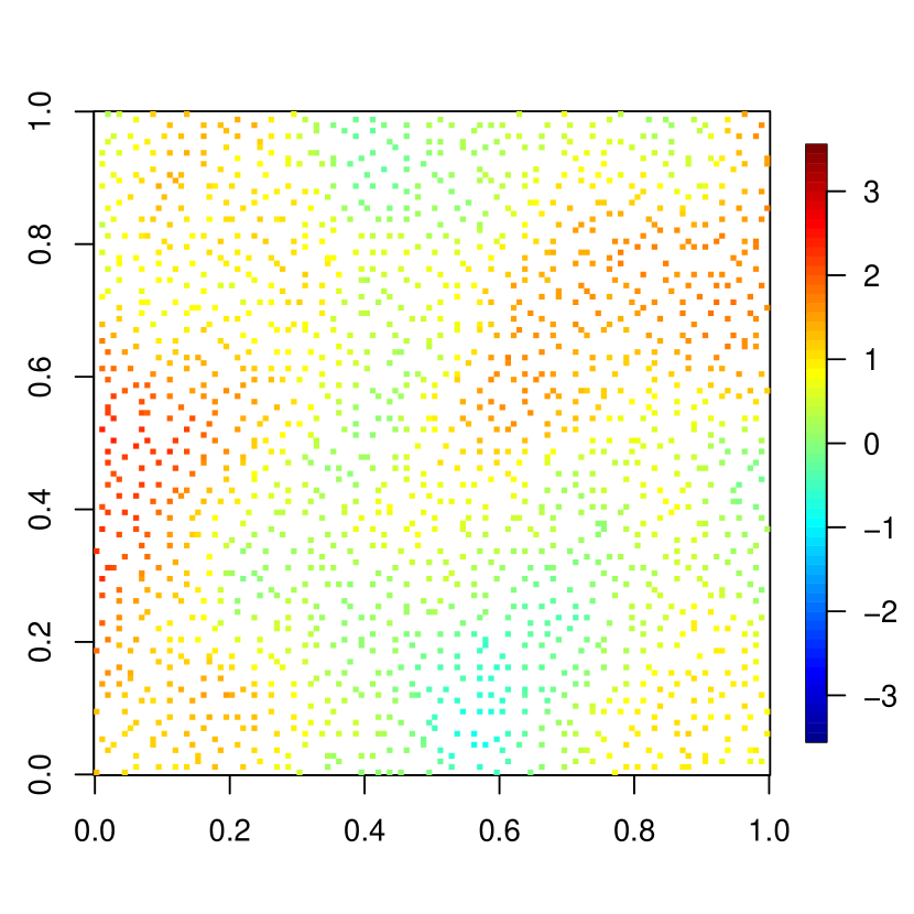
(f) (1, 0.3, 1)

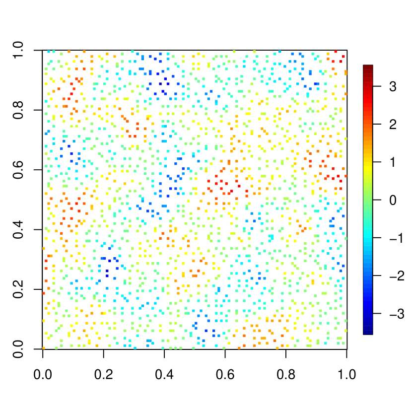
(g) (1, 0.03, 2)

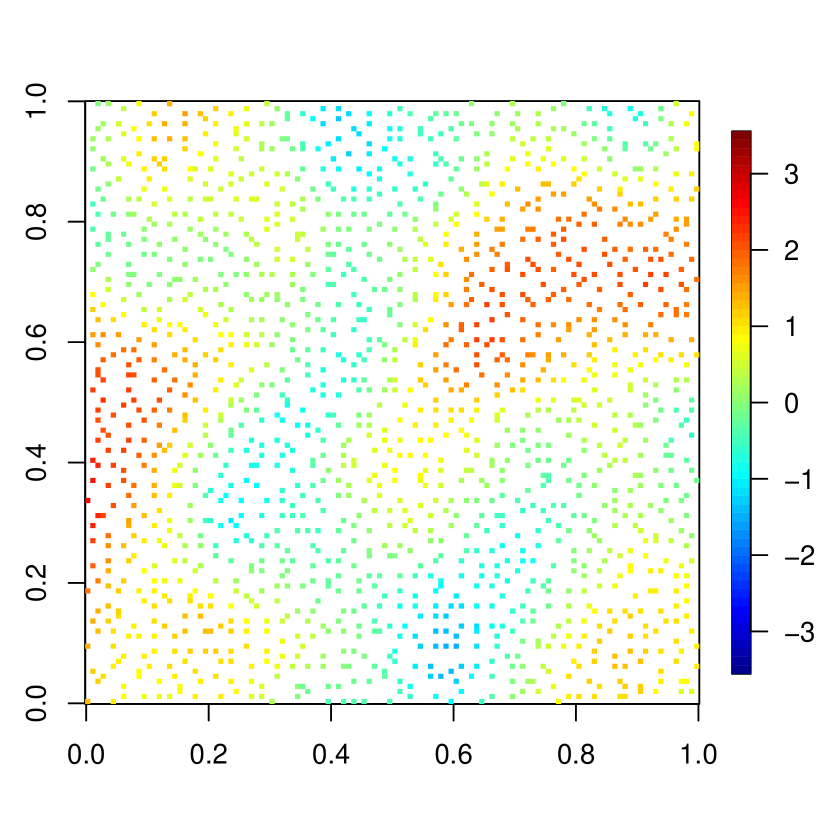
(h) (1, 0.1, 2)

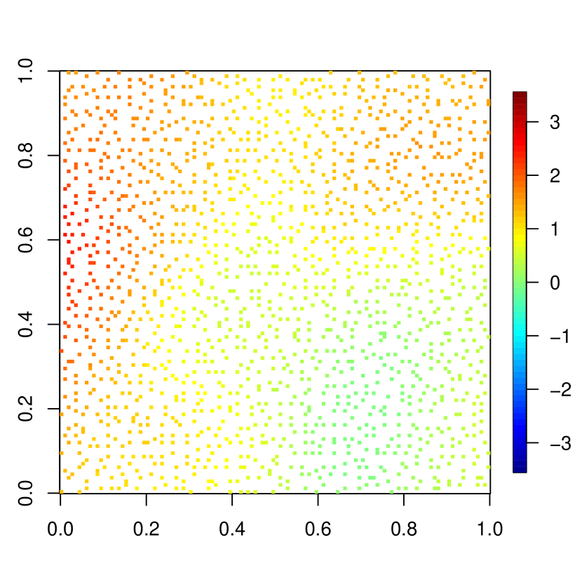
(i) (1, 0.3, 2)

Figure 3: Data simulated using ExaGeoStatR with univariate Matérn stationary covariance function in ($\sigma^{2}$, $\beta$, $\nu$) form at $1600$ geospatial locations in the unit square.

For comparison purpose, we also show how the sim.rf function of fields and the grf function of GeoR generate similar GRFs:

⬇

> library(geoR)

> sims = grf(n = 1600, grid = "reg", cov.pars = c(1, 0.1), kappa = 0.5)

> data.geoR.reg = list(x = sims$coords[, 1], y = sims$coords[, 2], z = sims$data)

⬇

> library(fields)

> sigma_sq = 1

> grid = list(x = (1 : 40) / 20,y = (1 : 40) / 20)

> xy = expand.grid(x=(1 : 40) / 20, y=(1 : 40) / 20)

> obj = matern.image.cov(grid = grid, theta = 0.1, smoothness = 0.5, setup = TRUE)

> sims.fields = sqrt(sigma_sq) * sim.rf(obj)

> data.fields.reg = list(x = xy[, 1], y = xy[, 2], z = c(sims.fields))

As can be seen, the three packages offer different types of flexibility in terms of data generation. However, when the goal is to generate a large GRF on an irregular grid with more than $20$K locations, both the sim.rf function and the grf function are not feasible. The sim.rf function simulates a stationary GRF only on a regular grid, and the grf function shows memory issues for large size (i.e., Error:vector memory exhausted). On the other hand, the simulate_data_exact function can easily generate the GRF within one minute with the following code:

⬇

> n = 25600

> hardware = list(ncores = 4, ngpus = 0, ts = 320, pgrid = 1, qgrid = 1)

> exageostat_init(hardware)

> data.exageo.reg = simulate_data_exact(kernel = "ugsm-s", theta= c(1, 0.1, 0.5),

dmetric = "euclidean", n, seed = 0)

> exageostat_finalize()

Simulating data on a large scale requires enough memory and computation resources. Thus, we recommend the users be consistent when generating large datasets with the available hardware resources. We also provide a set of synthetic and real large spatial data examples that can be downloaded from https://ecrc.github.io/exageostat/md_docs_examples.html for experimental needs.

III-D Example 2: Performance on Shared Memory Systems for Moderate and Large Sample Size

To investigate the estimation of parameters based on the exact computation, we use the exact_mle function in ExaGeoStatR. On a shared memory system with a moderate sample size, the number of cores (ncores) and tile size (ts) significantly affect the performance (see Figure 4). The following code shows the usage of the exact_mle function and returns execution time per iteration for one combination of n, ncores and ts:

⬇

> hardware = list (ncores = 4, ngpus = 0, ts = 160, pgrid = 1, qgrid = 1)

> exageostat_init(hardware)

> data.exageo.reg = simulate_data_exact(kernel = "ugsm-s", theta= c(1, 0.1, 0.5),

dmetric = "euclidean", n = 1600, seed = 0)

> result = exact_mle(data.exageo.reg, kernel = "ugsm-s", dmetric = "euclidean", optimization =

list(clb = c(0.001, 0.001, 0.001), cub = c(5, 5, 5 ), tol = 1e-4, max_iters = 20))

> time = result$time_per_iter

> exageostat_finalize()

In the exact_mle function, the first argument, data = list{x, y, z}, is a list that defines a set of locations in two-dimensional coordinates, x and y, and the measurement z of the variable of interest. The $kernel$ input defines the required covariance function. Here, dmetric is a distance parameter, the same as in the simulate_data_exact function. The optimization list specifies the optimization settings including the lower and upper bounds vectors, clb and cub, tol is the optimization tolerance and max_iters is the maximum number of iterations to terminate the optimization process. The optimization function uses the clb vector as the starting point of the optimization.

The above example has been executed using three different sample sizes, 16 different numbers of cores, and four different tile sizes to assess the parallel execution performance of ExaGeoStatR. We visualize the results by using the ggplot function in ggplot2 [Wickham, 2016] as shown in Figure 4. The figure shows the computational time for the estimation process using a different number of cores up to 16 cores. The y-axis shows the total computation time per iteration in seconds, while the x-axis represents the number of cores. The three sub-figures show the performance with different $n$ values: 400, 900, and 1600. Different curves represent different tile sizes which impact the performance of different hardware architectures. The figure shows that on our Intel Sandy Bridge machine, the best-selected tile size is 100. Tiling helps parallel execution to achieve the highest performance by increasing the reuse of data already loaded from the main memory (RAM) to the processor cache and reducing the data movements from RAM to cache. So, obtaining the best tile size depends on the processor cache size. Moving a complete tile from RAM to cache should increase the computation efficiency of the underlying algorithm. However, small tiles can also impact performance by satisfying better load balancing between the running processes, making determining the best tile size tricky. The simplest way to obtain the best tile size is to tune it on new hardware architectures before running large problems. We recommend trying different tile sizes to get the best performance from the ExaGeoStatR package.

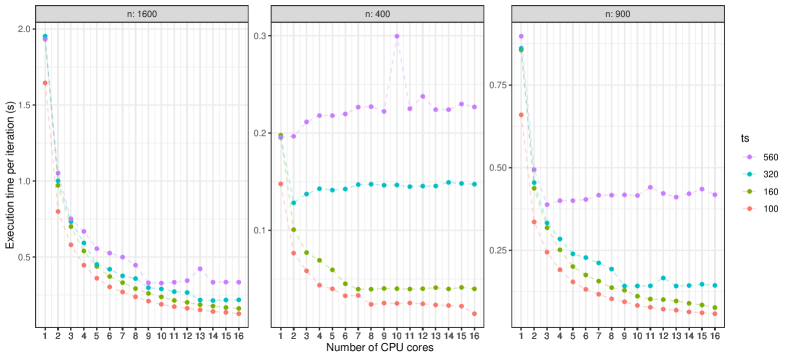
Figure 4: Parallel execution performance of ExaGeoStatR under different hardware settings. Each subfigure corresponds to a single sample size $n$ and shows the execution time in seconds per iteration with regards to the number of cores up to 16. Curves with different colors provide the effect of tile size (ts). (Red: ts=100. Green: ts=160. Blue: ts=320. Purple: ts=560).

After specifying the hardware environment settings, we test the accuracy of the likelihood-based estimation of ExaGeoStatR in comparison with GeoR and fields. The counterparts to the exact_mle function are likfit in GeoR and spatialProcess in fields. The simulated datasets from Example 1 are used as the input to assess the performance of parameter estimations. The synthetic datasets are generated on n=1600 points in $[0,1]\times[0,1]$. We take a moderate sample size that costs GeoR and fields approximately ten minutes to obtain enough results with different scenarios and iterations. The mean structure is assumed to be constantly zero across the region. One hundred replicates of samples are generated with different seed (seed$=1,\dots,100$) to quantify the uncertainty. We estimate the parameter values for each sample and obtain 100 sets of estimates independently. A Matérn covariance kernel is selected to generate the covariance matrix with nine different scenarios. Specifically, the variance is always chosen to be one, sigma_sq = 1.0, the spatial range takes three different values representing high, medium, and low spatial correlation, beta = c(0.3, 0.1, 0.03), and the smoothness also takes three values from rough to smooth, nu = c(0.5, 1, 2). The simulated datasets with moderate sample size are generated by the grf function. We choose the grf function in GeoR due to its flexibility in changing the parameter settings and in switching between regular and irregular grids. Herein, we depend on irregular grids to generate the data.

We set the absolute tolerance to $10^{-5}$ and unset the maximum number of iterations (max_iters = 0) to avoid non-optimized results. Hence, each package can show its best performance to estimate the correct value of each parameter. The simulated GRFs are generated by the grf function and stored as a list called data:

⬇

> library(geoR)

> sigma_sq = 1

> beta = 0.1 #choose one from c(0.3, 0.1, 0.03)

> nu = 0.5 #choose one from c(0.5, 1, 2)

> sims = grf(n = 1600, grid = "reg", cov.pars = c(sigma_sq, beta), kappa = nu)

> data = list(x = sims$coords[,1], y = sims$coords[,2], z = sims$data)

We have tried to keep the irrelevant factors as consistent as possible when comparing ExaGeoStatR with GeoR and fields. However, we identified some differences between the three packages that can hardly be reconciled. For example, GeoR estimates the mean structure together with the covariance structure, and fields does not estimate the smoothness parameter, $\nu$, in our package. In addition, in terms of the optimization methods, both GeoR and fields call the optim function in stats to maximize the likelihood function. The optim function includes six methods such as Nelder-Mead and BFGS. However, ExaGeoStatR uses the BOBYQA algorithm, which is one of the optimization algorithms of the sequential NLopt library in C/C++. The BOBYQA algorithm has the best performance in terms of MLE estimation. However, it is not available in the optim function. Table V lists the differences between the three packages.

Multiple algorithms are offered by the optim function and further implemented by GeoR and fields. However, many studies in the literature point out that the optim function is not numerically stable for a large number of mathematical functions, especially when a re-parameterization exists [Mullen et al., 2014, Nash et al., 2011, 2014]. Based on the 100 simulated samples, we show that ExaGeoStatR provides faster computation and gives more accurate and robust estimations with regards to the initial value and grid type.

We first estimate the parameters by exact_mle in ExaGeoStatR. We use the number of cores to be eight to reproduce the results on most machines. Users can specify their settings and optimize the performance by referring to the results in Figure 4. The final results also report the time per iteration, total time, and the number of iterations for each optimization:

⬇

> hardware = list (ncores = 8, ngpus = 0, ts = 100, pgrid = 1, qgrid = 1)

> exageostat_init(hardware)

> result = exact_mle(data, kernel = "ugsm-s", dmetric = "euclidean", optimization =

list(clb = c(0.001, 0.001, 0.001), cub = c(5, 5, 5 ), tol = 1e-4, max_iters = 20))

> para_mat = result$est_theta

> time_mat = c(result$time_per_iter, result$total_time, result$no_iters)

> exageostat_finalize()

Then we estimate the parameters under the same scenarios using the likfit function in GeoR and the spatialProcess function in fields. For GeoR and fields, the chosen optimization options are method = c("Nelder-Mead"), abstol = 1e-5, and maxit = 500, where the maximum number of iterations set as 500 could never be reached. Because fields does not optimize the smoothness, $\nu$, so we set it as the true value (an advantageous favor for fields). GeoR has to optimize the mean parameter, at least a constant, but it is treated to be independent of the covariance parameters as the mean value of data. In addition, to accelerate the optimization of fields, we minimize the irrelevant computation by setting gridN = 1:

⬇

> result = spatialProcess(x = cbind(data$x,data$y), y = data$z,

cov.args = list(Covariance = "Matern", smoothness = nu), gridN = 1, reltol = 1e-05)

> para_mat = c( result$MLESummary[[7]],result$MLESummary[[8]], result$args$smoothness)

> time_mat = c(result$timingTable[3,2]/dim(result$MLEJoint$lnLike.eval)[1],

result$timingTable[3,2], dim( result$MLEJoint$lnLike.eval)[1])

Using the GeoR package:

⬇

> time = system.time( fit_obj <- likfit( coords = cbind(data$x, data$y),

data = data$z, trend = "cte", ini.cov.pars = c(0.001, 0.001), fix.nugget = TRUE,

nugget = 0, fix.kappa = FALSE, kappa = 0.001, cov.model = "matern", lik.method = "ML",

limits = pars.limits(sigmasq = c(0.001, 5), phi = c(0.001, 5), kappa = c(0.001, 5)),

method = "Nelder-Mead", control = list(abstol = 1e-5, maxit = 500)))[3]

> time_mat = c(time / fit_obj$info.minimisation.function$counts[1],

time, fit_obj$info.minimisation.function$counts[1])

> para_mat = c(fit_obj$sigmasq, fit_obj$phi, fit_obj$kappa)

The computational efficiency is compared based on the average execution time per iteration and the average number of iterations. As shown in Table VI, the running time per iterations of ExaGeoStatR is about 12X and 7X faster than GeoR and fields, respectively. The running time per iteration is robust between different scenarios. Since fields does not estimate the smoothness parameter, it runs faster than GeoR. Although GeoR also estimates an extra constant mean parameter, it does not affect the computation much because the mean parameter is simply the mean of the measurements z and is estimated separately. Table VI also shows the number of iterations to reach the tolerance. We can see that ExaGeoStatR requires more iterations but much less time to reach the accuracy.

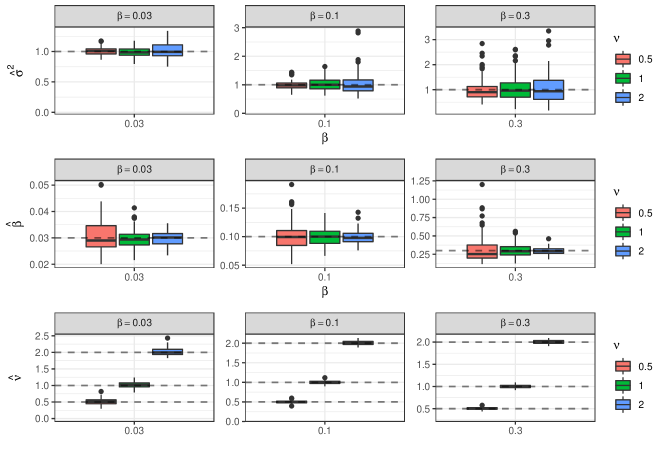
Figure 5: The estimation accuracy of ExaGeoStatR with different sets of parameter vectors. Each row shows the estimation of a parameter among variance, $\sigma^{2}$, spatial range, $\beta$, and smoothness, $\nu$. Each column corresponds to one setting of spatial range, $\beta$, and the color of the boxplots identifies a type of smoothness, $\nu$. True values are represented by a horizontal dashed line.

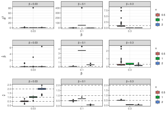
Figure 6: The estimation accuracy of GeoR with different sets of parameter vectors.

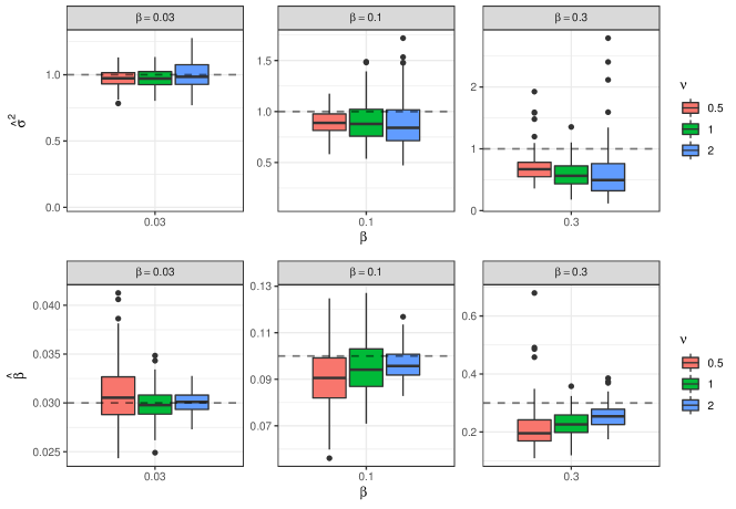
Figure 7: The estimation accuracy of fields with different sets of parameter vectors. The results related to fields only have two rows since the package does not estimate $\nu$.

Figures 5, 6, and 7 show the estimation accuracy between the three packages using boxplots. It is clear that ExaGeoStatR outperforms GeoR and fields. Together with Table VI, we can see that ExaGeoStatR requires more iterations when $\nu$ increases since we set the initial values to be 0.001 for all scenarios. It implies that even under the circumstance of bad initial values, e.g., $\nu=2$ and $\beta=0.3$, ExaGeoStatR can reach the global maximum by taking more iterations. However, the estimation performance of both GeoR and fields becomes worse when the initial values deviate from the truth. In particular, GeoR reaches a local maximum only after about 20 iterations for medium and large smoothness and spatial range, so that its estimated values are even not inside the range of fields and ExaGeoStatR.

The result is mainly due to the numerical optimization of $\nu$, which involves the non-explicit Bessel function in the Matérn kernel. Therefore, fields has a more robust estimation because it does not estimate the smoothness (we fix it as the truth), although fields calls the same optim function as GeoR. However, even though ExaGeoStatR estimates the smoothness parameter, our package still outperforms fields in terms of $\beta$ and $\sigma^{2}$, especially for medium and large spatial range correlation.

Other optimization methods rather than “Neader-Mead” are also explored, such as the default optimization option of fields, “BFGS”. As a quasi-Newton method, “BFGS” is fast but not stable in many cases. Similar to the worst result of GeoR, the optimization jumps out after only a few steps and reports incorrect results even with a decent guess of initial values. Even worse, both GeoR and fields report errors in computing the inverse of the covariance matrix (i.e., Error:error in solve.default(v$varcov, xmat):system is computationally singular).

The experiment above shows that the optim function used by both GeoR and fields is not stable with regards to the initial values, no matter what algorithm we choose. In addition, by simulating GRFs on an irregular grid (grid = "irreg"), few simulated GRFs can get the output without any error. For data on an irregular grid, locations can be dense so that the distances between certain points are very close to each other. Therefore, the columns of the covariance matrix corresponding to the dense locations can be numerically equal. For the data on a unit square, we find that ExaGeoStatR may only have the singularity problem when the closest distance is less than 1e-8. On the contrary, the problem occurs when the smallest distance is close to 1e-4 for fields and GeoR. As a result, although ExaGeoStatR is designed to provide a faster computation by making use of manycore systems, the optimization algorithm it is based upon gives a more accurate and robust estimation than any algorithm in the optim function.

We also investigate the computational time of the three packages as $n$ increases. The hardware settings remain the same for ExaGeoStatR with 8 CPU cores. The max number of iterations is set to 20 for all three packages to accelerate the estimation. The results report the total computational time. The tested number of locations ranges from 100 to 90,000. However, both GeoR and fields take too much time when $n$ is large. For example, the estimation with GeoR for 22,500 locations requires more than 17 hours. Thus we stop the simulation for GeoR and fields at the size of 22,500 and only show the execution time of ExaGeoStatR for larger $n$ with 8 CPU cores. The results are shown in Figure 8. It can be seen that, when $n=22,500$, ExaGeoStatR is 33 times faster than fields and 92 times faster than GeoR.

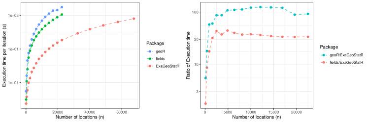
Figure 8: The execution time per iteration as $n$ increases for GeoR, fields, and ExaGeoStatR with 8 CPU cores. The covariance parameters are set to be $(\sigma^{2},\beta,\nu)=(1,0.1,0.5)$. Each curve on the left panel shows the exact running time per iteration of one package, and each curve on the right panel gives the ratio of execution time compared to ExaGeoStatR. The $y$-axis is shown in $\log_{10}$ scale.

III-E Example 3: Extreme Computing on GPU Systems

Since the main advantage of ExaGeoStatR is the multi-architecture compatibility, here we provide another example of using ExaGeoStatR on GPU systems. We choose the number of locations ranging from 1600 to approximately 100K. The R code below shows an example of how to use 26 CPU cores and 1 GPU core with $n=25{,}600$:

⬇

> n = 25600

> hardware = list (ncores = 26, ngpus = 1, ts=960, pgrid=1, qgrid=1)

> exageostat_init(hardware)

> data = simulate_data_exact(kernel = "ugsm-s", theta = c(1, 0.1, 0.5),

dmetric = "euclidean", n, seed = 0)

> result_cpu = exact_mle(data, kernel = "ugsm-s", dmetric = "euclidean", optimization =

list(clb = c(0.001, 0.001, 0.001), cub = c(5, 5, 5 ), tol = 1e-4, max_iters = 20))

> time_cpu = result_cpu$time_per_iter

> exageostat_finalize()

The above code shows that ExaGeoStatR has a user-friendly interface to abstract the underlying hardware architecture to the user. The user needs only to specify the number of cores and GPUs required for one’s execution. Figure 9 reports the performance with different numbers of GPU accelerators: 1, 2, and 4. The figure also shows the curve using the maximum number of cores (28-core) on the machine without GPU support. The figure demonstrates how GPUs speed up the execution time compared to CPU-based running. Moreover, the figure shows the scalability using different numbers of GPUs.

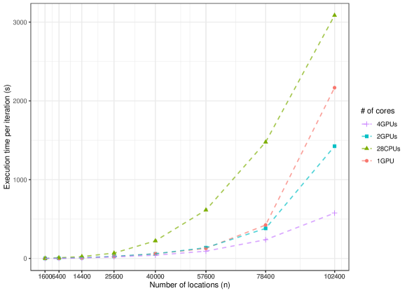
Figure 9: Execution performance of ExaGeoStatR under different CPU and GPU combinations. The covariance parameters are set to be $(\sigma^{2},\beta,\nu)=(1,0.1,0.5)$. Each curve corresponds to the execution time per iteration with regards to different sample sizes, $n$.

III-F Example 4: Extreme Computing on Distributed Memory Systems

This subsection gives an example of using ExaGeoStatR on distributed memory systems (i.e., supercomputer Shaheen II Cray XC40). As for shared memory and GPU systems, the ExaGeoStatR package abstracts the underlying hardware to a set of parameters. With distributed systems, the user needs to define four main parameters: pgrid and qgrid which represent a set of nodes arranged in a pgrid $\times$ qgrid rectangular array of nodes (i.e, two-dimensional block-cyclic distribution), ncores which represents the number of physical cores in each node, and ts which represents the optimized tile size. Another example of the usage of ExaGeoStatR on a distributed memory system with 31 CPU cores, $4\times 4$ rectangular array of nodes, ts=960 and, n=250,000 is shown below:

⬇

> n = 250000

> hardware = list (ncores = 31, ts=960, pgrid=4, qgrid=4)

> exageostat_init(hardware)

> data = simulate_data_exact(kernel = "ugsm-s", theta = c(1, 0.1, 0.5),

dmetric = "euclidean", n, seed = 0)

> result_cpu = exact_mle(data, result_cpu = exact_mle(data, kernel = "ugsm-s",

dmetric = "euclidean", optimization = list(clb = c(0.001, 0.001, 0.001),

cub = c(5, 5, 5 ), tol = 1e-4, max_iters = 20)

> time_cpu = result_cpu$time_per_iter

> exageostat_finalize()

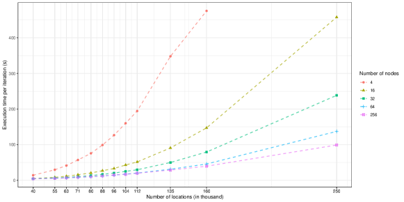
Figure 10: Performance of ExaGeoStatR using different numbers of nodes. The time per iteration is averaged over $20$ iterations. The realization is generated from a zero-mean GRF under the Matérn covariance structure with the parameters $(\sigma^{2},\beta,\nu)=(1,0.1,0.5)$.

Figure 10 shows the performance results of running different problem sizes on Shaheen II Cray XC40 using different numbers of nodes. The distribution of the nodes are $2\times 2$, $4\times 4$, $8\times 4$, $8\times 8$, and $16\times 16$. The figure shows strong scalability of ExaGeoStatR with different numbers of nodes up to 64 nodes. The reported performance is the time per iteration averaged over $20$ iterations with settings:

⬇

> export STARPU_SCHED = eager.

> export STARPU_LIMIT_MIN_SUBMITTED_TASKS = 9000.

> export STARPU_LIMIT_MAX_SUBMITTED_TASKS = 10000.

III-G Example 5: ExaGeoStatR Versus bigGP on Distributed Systems

This subsection gives an example of using ExaGeoStatR on the Ibex HPC cluster from KAUST (https://www.hpc.kaust.edu.sa/ibex) using up to 16 40-core Intel Skylake and 40-core Intel Cascadelake nodes. We intend in this example to compare ExaGeoStatR with bigGP from a performance perspective on a distributed system. We focus on the performance of the Cholesky factorization operation since it is the most time-consuming operation when evaluating the likelihood function. We rely on the Matérn covariance function to build the target covariance matrix.

As in Example 4, the user needs to define four main parameters to be able to run ExaGeoStatR script on distributed systems: pgrid and qgrid which represent a set of nodes arranged in a pgrid $\times$ qgrid rectangular array, ncores which represents the number of cores used in each node, and ts, which represents the tuned tile size.

The bigGP package uses $RMPI$ [Yu, 2002], an MPI interface in R, to perform the GP modeling in a distributed manner. Below is an example of bigGP code to calculate the Cholesky factorization for a given matrix that can be executed on distributed-memory systems:

⬇

> library("bigGP")

> p = 4

> bigGP.init(p-1)

> m = 100

> gd <- seq(0, 1, length = m)

> locs = expand.grid(x = gd, y = gd)

> theta <- c(1, 0.1, 0.5)

> mpi.bcast.Robj2slave(theta)

> mpi.bcast.Robj2slave(covfunc)

> mpi.bcast.Robj2slave(locs)

> mpi.bcast.cmd(indices <- localGetTriangularMatrixIndices(nrow(locs)))

> mpi.bcast.cmd(C <- covfunc(theta, locs, indices))

> remoteLs()

> remoteCalcChol('C', 'L', n = m^2)

> bigGP.quit()

Here $p$ represents the total number of nodes to run the script. bigGP relies on one master process and $p-1$ slave processes. The user has to submit the jobs with $p$ processes. In line 3, a bigGP instance is initiated using 3 slaves nodes. $n$ represents the number geospatial locations where $n=m^{2}$. $locs$ is the set of locations, and $theta$ is the parameter vector to use with a predefined covariance function kernel. The $remoteCalcChol$ function is the Cholesky factorization function in the bigGP package.

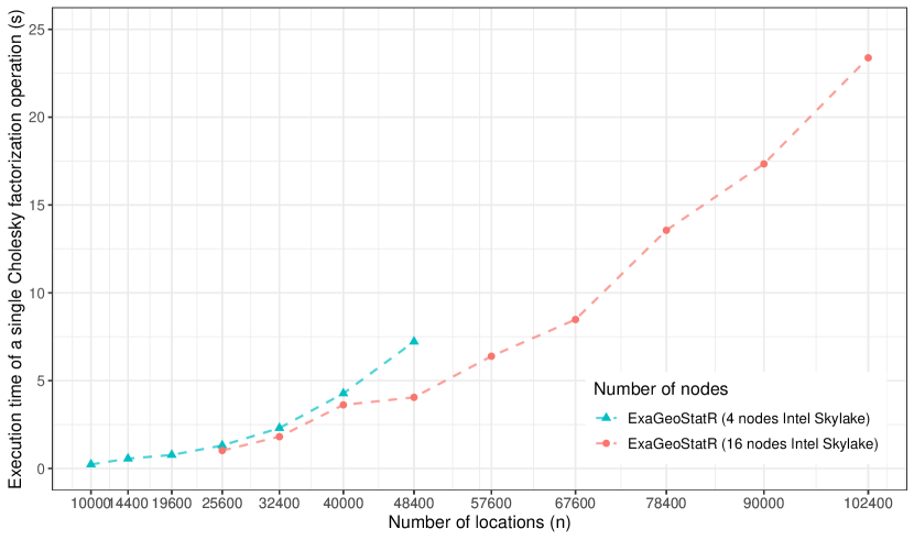
(a) ExaGeoStatR on Intel Skylake

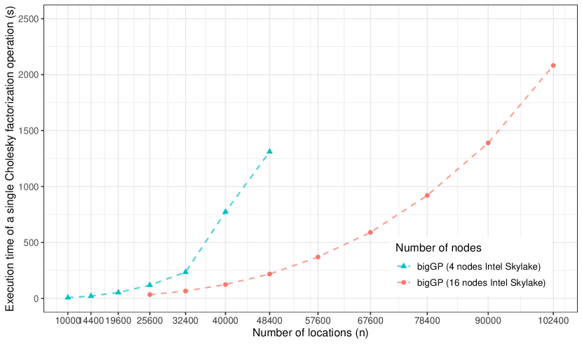
(b) bigGP on Intel Skylake

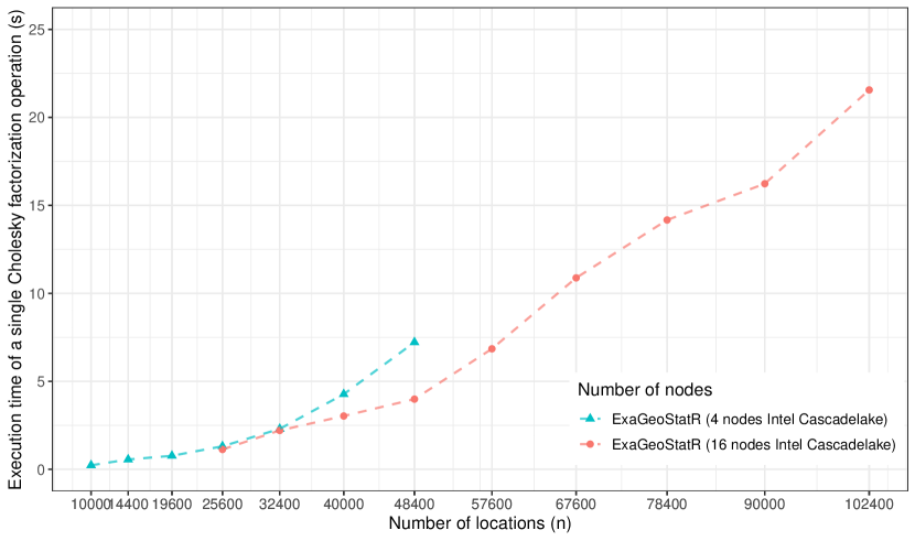
(c) ExaGeoStatR on Intel Cascadelake

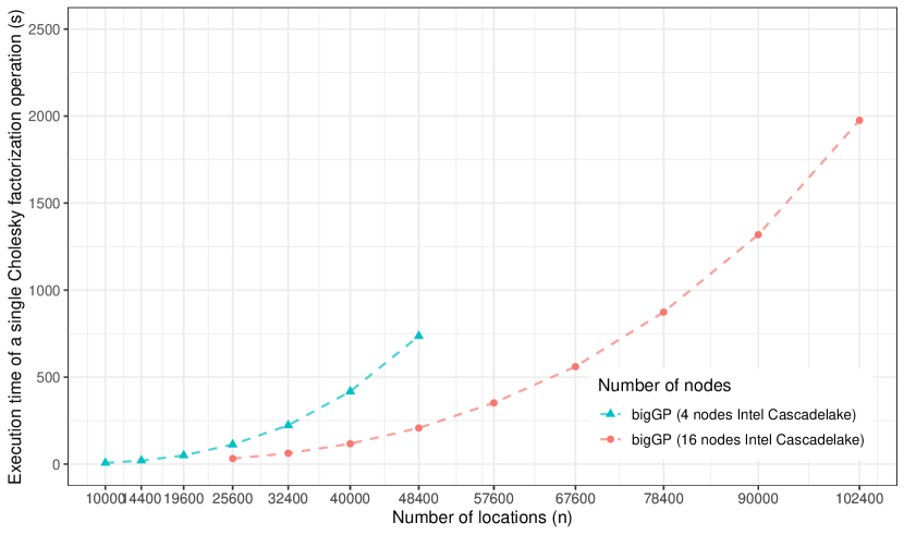
(d) bigGP on Intel Cascadelake

Figure 11: Performance of the Cholesky factorization operation using ExaGeoStatR (a-c) and bigGP (b-d) packages on 4 and 16 nodes on the KAUST Ibex HPC Cluster, where each node is a 40-core Intel Skylake/Cascadelake processors.

Due to the high network congestion of the cluster, we repeated each run five times and selected the best execution time for both ExaGeoStatR and bigGP. Figure 11 shows the execution time for running a single Cholesky factorization on 4 and 16 Intel Skylake/Cascadelake nodes using the Ibex cluster. The figure shows how both ExaGeoStatR and bigGP can take advantage of increasing the number of nodes to improve the overall performance of the Cholesky factorization. On both architectures, it is demonstrated that ExaGeoStatR outperforms bigGP using a different number of nodes which shows the benefits of tile-based parallel solvers and runtime systems compared to the block-based parallel solvers and pure OpenMP/MPI implementation.

IV Application to Sea Surface Temperature Data: A tutorial

West-blowing trade winds in the Indian Ocean push warm surface waters against the eastern coast of Africa. These waters move south along the coastline, eventually spilling out along the Indian and Atlantic Oceans boundary. This jet of warm water, known as the Agulhas Current, collides with the cold, west-to-east-flowing Antarctic Circumpolar Current, producing a dynamic series of meanders and eddies as the two waters mix. The result makes for an interesting target for spatial analysis that we illustrate as a tutorial.

This application study provides an example where the MLE is computed in high dimensions, and ExaGeoStatR facilitates the procedure on many-core systems. We use the sea surface temperature collected by satellite for the Agulhas and surrounding areas off the shore of South Africa. The data covers 331 days, from January 1 to November 26, 2004. The region is abstracted into a $72\times 240$ regular grid, with the grid lines denoting the latitudes and longitudes and the spatial resolution is approximately $25$ kilometers, though exact values depend on latitude. Although fields and geoR do not have input dimension limits, the computation with ExaGeoStatR has a distinct advantage on parallel architectures, hence more suitable for MLE with more optimization iterations to reach convergence.

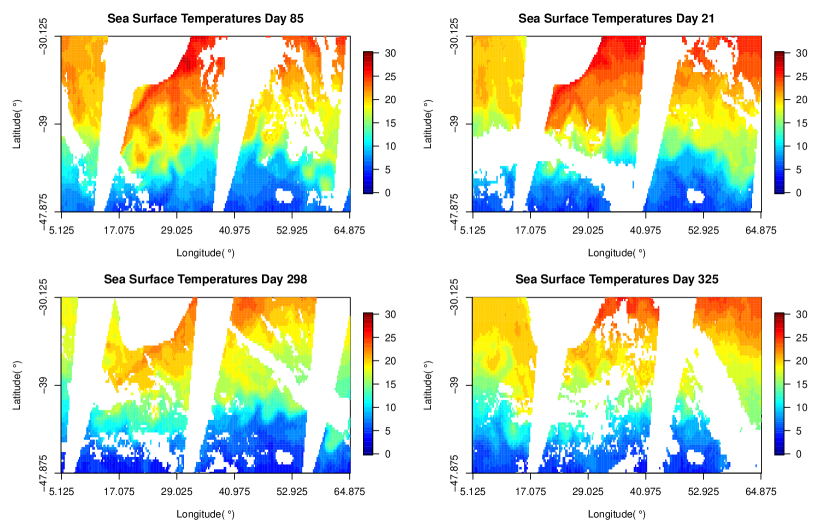
(a)

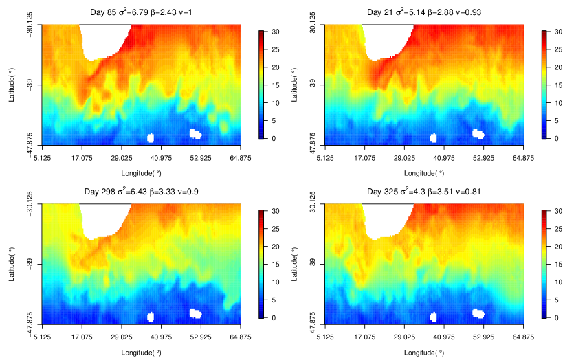
(b)

Figure 12: Panels (a) are the original sea surface temperatures in Celsius (°C) where the locations with NA values are colored in white. Panels (b) are the predicted sea surface temperatures in Celsius (°C) based on the linear mean structure and the kriging results where the land area is not predicted and colored in white. Parameter estimates are provided for each panel.

Our analysis considers only the spatial structure in the spatio-temporal dataset and hence, assumes independence between the parameters on different days. Before introducing our model, we first present some exploratory data analysis. In Figure 12(a), we use the image.plot function from the fields package to plot the heatmap of the sea surface temperature on selected four days that are also used for showing the kriging results later. Numerous gaps are present in the data, corresponding to three main causes: 1) land: specifically South Africa and Lesotho, visible in the left-center of the top of the plot, as well as two small islands towards the southern boundary; 2) clipping: the large wedge-shaped voids cutting N-S across the picture resulting from the satellite’s orbital path; and 3) cloud cover: all or most of the remaining swirls and dots present in the image. Various forms of kriging can be used to attempt to fill those gaps caused by orbital clipping and cloud cover. Of course, it does not make sense to estimate sea surface temperatures for gaps caused by the presence of land. A pronounced temperature gradient is visible from highs of over 25^∘ C in the north of the study area to a low of 3.5^∘ C towards the southern boundary. This indicates spatial correlation in the dataset, but it also shows that the data are not stationary, as the mean temperature must vary considerably with latitude.

We plot the mean and standard deviation along each latitude on the four days in Figure 13.

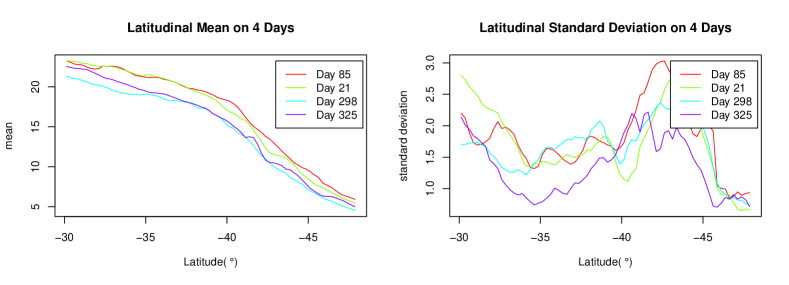
Figure 13: Exploratory data analysis on Days 85, 21, 298, and 325. The mean and standard deviation are computed with missing values removed.

The longitudinal mean and standard deviation (not shown) are relatively stable, although there are spikes and troughs due to the missing data. Since the locations are sufficient for a regression with only three parameters, we also include the longitude as a regression variable and assume the following linear model with Gaussian noise for the sea surface temperature, $T(\lambda,\alpha)$:

$$T(\lambda,\alpha) =\mu(\lambda,\alpha)+\epsilon(\lambda,\alpha;\sigma^{2},\beta,\nu),$$

$$\mu(\lambda,\alpha) =c+a\cdot\lambda+b\cdot\alpha,$$

where $\lambda$ denotes longitude, $\alpha$ denotes latitude, and $\epsilon(\lambda,\alpha)$ is a GRF with zero mean and a Matérn covariance structure parameterized as in (3). Here, $a$, $b$, and $c$ are the linear coefficients for the mean structure, which we compute prior to the covariance structure based on the least square estimation. Maximum likelihood estimation is only applied to $\sigma^{2},\beta$, and $\nu$ at the second stage because non-convex optimization for six parameters requires a larger sample size and significantly more iterations. The original data have different proportions of missing values, varying from Day 1 to Day 331. We ignore those days whose missing value proportion exceeds $50\%$ so that the number of predictions is not more than the original number of observations.

The model fitting is done with the exact_mle function from the ExaGeoStatR package, which maximizes the exact likelihood. Specifically, the function call is:

⬇

> x = x[!is.na(z)]

> y = y[!is.na(z)]

> z = z[!is.na(z)]

> mydf = data.frame(x, y, z)

> mymdl = lm(formula = z ~ x + y , data = mydf)

> z = as.numeric(mymdl$residuals)

> mytime = system.time(theta_out = exact_mle(data, kernel = "ugsm-s",

dmetric = "euclidean", optimization = list(clb = c(0.001, 0.001, 0.001),

cub = c(5, 5, 5 ), tol = 1e-4, max_iters = 20))[3]

Referring to Section III, n is the number of spatial locations, ncore and ngpu are the numbers of CPU cores and GPU accelerators to deploy, ts denotes the tile size used for parallelized matrix operations, pgrid and qgrid are the cluster topology parameters, x and y store either the Cartesian coordinates or the spherical coordinates of the geometry, z is one realization of the spatial variables of dimension n, clb and cub define the search range for the three parameters, dmetric is a boolean indicating whether the Euclidean distance or the great circle distance is used for the covariance matrix, tol and niter specify the stopping criteria which supports both a tolerance level for reckoning convergence and the maximum number of iterations. This application study uses $16$ Intel Sandy Bridge Xeon E5-2650 processors without any GPU acceleration.

The tile size is initialized at $160$, and the grid dimensions are both $1$ for simplicity. In order to compare with the geoR and fields packages, we set niter to $20$ and measure the time cost of fitting the GRF to the data on Day 1, which has over $8{,}800$ valid (not NA) locations. The following is the code calling the likfit and spatialProcess functions while the function call for exact_mle was already shown above:

⬇

> time = system.time(fit_obj = spatialProcess(cbind(x, y), z, cov.args = list(

Covariance = "Matern", smoothness = 0.8), verbose = T, theta.start = 0.1,

theta.range = c(0.1, 5), optim.args = list(method = "Nelder-Mead",

control = list(maxit = 20, tol = 1e-4))))[3]

> data_obj = as.geodata(cbind(x, y, z))

> time = system.time(fit_obj = likfit(geodata = data_obj, trend = "cte",

ini.cov.pars = c(0.1, 0.1), fix.nugget = TRUE, nugget = 0, fix.kappa = FALSE,

kappa = 0.1, cov.model = "matern", lik.method = "ML", limits = pars.limits(

sigmasq = c(0.01, 20), phi = c(0.01, 20), kappa = c(0.01, 5)), print.pars = TRUE,

method = "Nelder-Mead", control = list(maxit = 20,abstol = 1e-4)))[3]

The exact_mle function was executed with $15$ CPUs and took $147$ seconds, the likfit function from the geoR package cost $2{,}286$ seconds, and the spatialProcess function from the fields package needed $4{,}049$ seconds. It usually requires more than $100$ iterations to reach convergence, which renders the geoR and fields packages very difficult to use for fitting high-dimensional GRFs, whereas the ExaGeoStatR package utilizes parallel architectures and reduces the time cost by more than one order of magnitude. Hence, ExaGeoStatR allows to fill many spatial images quickly.

We select $(0.01,20.0)$ as the searching range for $\sigma^{2}$ and $\beta$ and $(0.01,5.00)$ for $\nu$ to guarantee the results not landing on boundary values. The initial values for all three parameters are the corresponding lower bounds of the searching ranges by default, and the optimization continues without any limit on the number of iterations until convergence is reached within a tolerance level of $10^{-4}$. There are $174$ days whose missing value percentages are below $50\%$, and Table VII summarizes the independently-estimated parameters for these days.

Here, $\nu$ has the most consistent estimations among the three parameters while $\sigma^{2}$ and $\beta$ have similar variability. Based on the estimated parameters, we predict the sea surface temperature at locations where the data are missing with kriging, which computes the conditional expectation using a global neighborhood. The kriging is done with exact_predict() from the ExaGeoStatR package as indicated below:

⬇

> hardware = list (ncores = 2, ngpus = 0, ts = 320, pgrid = 1, qgrid = 1)

> exageostat_init(hardware)

> Data_train_list <- list("x" = x_known, "y" = y_known, "z" = z_known )

> Data_predict_list <- list("x" = x_unknown, "y" = y_unknown)

> prediction_result <- exact_predict(Data_train_list,

Data_predict_list,"ugsm-s", dmetric, est_theta, 0)

> exageostat_finalize()

In Figure 12 we show the original and the predicted sea surface temperature for the four days corresponding to the $99\%$, $66\%$, $33\%$, and $1\%$ quantiles of the estimated $\nu$ to visualize the smoothness change. Day 85 seemingly has more details than Day 325, although the main factor governing the temperature change is the mean structure.

V Discussion

Statistical modeling methods have been widely used to analyze and understand the behavior of geospatial data in environmental data science applications. For example, the Maximum Likelihood Estimation (MLE) is used to model environmental data by building a covariance matrix to describe the relations between the observations at geographical locations. This operation has $O(n^{3})$ computation complexity and $O(n^{2})$ memory complexity due to the need to perform an inverse function to a generated covariance matrix with dimension equal to the number of locations, $n$.

Environmental data have increased tremendously in size due to recent advances in observational techniques and existing tools cannot easily handle them, especially in the statisticians’ preferred programming environment, i.e., R. Therefore, in this work, we tackled the computational complexity of the MLE operation on large-scale systems within the R environment. We presented the ExaGeoStatR package that allows large-scale geospatial modeling and prediction using the MLE operation. By exploiting the current state-of-the-art parallel linear algebra solvers and dynamic runtime systems, ExaGeoStatR can compute the Gaussian maximum likelihood function on different parallel architectures (i.e., shared memory, GPUs, and distributed systems). Large-scale Gaussian calculations in R become possible with ExaGeoStatR by mitigating its memory space and computing restrictions.

The ExaGeoStatR package provides four options to evaluate the MLE operation, i.e., exact, Diagonal Super-Tile (DST), Tile Low-Rank (TLR), and Mixed-Precision (MP). However, this work was only concerned with analyzing and assessing the performance of the exact computation variant (the focus of comparison in this paper) against existing well-known R packages, such as GeoR and fields. We focused on exact computations to highlight the parallel capabilities of ExaGeoStatR with the exact solution over the aforementioned R packages and its ability to run on different hardware architectures. Of course, parallelizing the approximation methods and scaling them on a large system will allow crossing the memory threshold of these methods with large problem sizes. However, we did not cover the approximation capabilities of ExaGeoStatR since it was well-covered in previous studies [Abdulah et al., 2018a, b, 2019, Hong et al., 2021, Abdulah et al., 2022b].

The evaluation demonstrates a significant difference in ExaGeoStatR performance compared to the other two packages. The accuracy evaluation also shows that ExaGeoStatR performs very well on synthetic datasets compared to GeoR and fields. The evaluations of the other ExaGeoStatR computation methods (DST, TLR, MP) can be found in Abdulah et al. [2018a, b, 2019, 2022b]. ExaGeoStatR also includes seven covariance functions. In this work, we evaluated the performance of univariate stationary Gaussian random fields with Matérn covariance function. Other studies include the evaluation of other covariance functions such as multivariate models [Salvana et al., 2021], and space-time models [Salvaña et al., 2022]. ExaGeoStatR can also include a nugget effect in all of its kernels.

We aimed from the beginning to abstract the parallel execution functions away from the concerns of the R developer. The developer only needs to specify some parameters to define the underlying hardware architecture and the package will automatically optimize the execution on the target hardware through the internal runtime system. In this way, we improve the portability of our software and make it more suitable for the R community developers. The current version of ExaGeoStatR only supports a zero mean to provide a robust and efficient estimation of covariance. However, the package can also be helpful in many other problems. First, when the mean function is not zero, the simplest approach is to estimate the mean and the covariance function independently, as we did in the application tutorial. Theoretically, this independent maximum likelihood estimation will result in a biased random effect and can be improved by the restricted maximum likelihood (REML) techniques. However, as fields suggests, using REML typically does not make much difference. Second, we can predict at new locations (kriging) with uncertainties once the covariance parameters are estimated. The prediction is calculated by the conditional distribution of the multivariate Gaussian. Third, even when spatial nonstationarity is observed, we can still apply ExaGeoStatR by assuming local stationarity. This idea is implemented in convoSPAT [Risser and Calder, 2017]. Once we obtain the estimated parameters locally, we can reconstruct the nonstationary covariance function. Finally, ExaGeoStatR is also useful for space-time and multivariate GRFs, where the covariance function we use should be replaced by a spatio-temporal covariance function and a cross-covariance function, respectively. As for our future work, ExaGeoStatR will provide the necessary built-in functions to support the extensions mentioned above for more complex applications.

VI Acknowledgment

The research in this manuscript was supported by funding from the King Abdullah University of Science and Technology (KAUST) in Thuwal, Saudi Arabia. We would like to thank the Supercomputing Laboratory (KSL) at KAUST for providing the hardware resources used in this work, including the Ibex cluster and Shaheen-II Cray XC40 supercomputer. Finally, the authors would like to thank Bilel Hadri and Greg Wickham from the KSL team for their valuable help in running the experiments in this publication.

Appendix: ExaGeoStatR Installation Tutorial

Herein, we provide a detailed description of how to install the ExaGeoStatR package with different capabilities. ExaGeoStatR is currently supported on both macOS and Linux systems. To automatically compile several dependencies, ExaGeoStatR requires a source of BLAS, CBLAS, LAPACK and LAPACKE routines (e.g., Intel MKL and OpenBLAS) that must be available on the system before installing ExaGeoStatR. The package is hosted in a GitHub repository and can be downloaded and installed directly from there. The ExaGeoStatR package is available through https://github.com/ecrc/exageostatR GitHub repository. We also provide an ExaGeoStatR docker image to increase the reusability of the package. The docker image can be found at https://hub.docker.com/r/ecrc/exageostat-r.

ExaGeoStatR includes a self-installation configuration file that helps the user installation of different software dependencies as mentioned in Section II. Thus, to directly install ExaGeoStatR from GitHub:

⬇

> install.packages("devtools")

> library("devtools")

> install_git(url = "https://github.com/ecrc/exageostatR")

The $install\_git$ command can be edited to change the default configuration of the ExaGeoStatR package to support several installation modes:

• To enable MPI support for distributed memory systems (i.e., an MPI library should be available on the system (e.g. MPICH, OpenMPI, and IntelMPI)):

  ⬇

  > install_git(url = "https://github.com/ecrc/exageostatR",

  configure.args = c('–enable-mpi'))

• To enable CUDA support for GPU systems (i.e., the CUDA library should be available on the system):

  ⬇

  > install_git(url = "https://github.com/ecrc/exageostatR",

  configure.args = c('–enable-cuda'))

• If all ExaGeoStatR software dependencies have been already installed on the system (i.e., install ExaGeoStatR package without dependencies):

  ⬇

  > install_git(url = "https://github.com/ecrc/exageostatR",

  configure.args = c('–no-build-deps'))

The Docker image can be also an easy way to use the ExaGeoStatR package but the performance could be impacted on different hardware architectures. The Docker pull command for ExaGeoStatR package is:

⬇

docker pull ecrc/exageostat-r

To independently install ExaGeoStatR dependencies, the user can follow the complete installation guide at: https://github.com/ecrc/exageostatR/blob/master/InstallationGuide.md

TABLE I: Comparison of some existing Gaussian process software.

Package	Platform	Version	Exact Calc.	Approx. Calc.	Supports Parallel Execution	Reference
bigGP	R	V0.1-7	✓	✗	✓	[Paciorek et al., 2015]
ExaGeoStatR	R	V1.0.1	✓	✓	✓	This work
fields	R	V14.1	✓	✗	✗	[Nychka et al., 2017]
GeoR	R	V1.9-2	✓	✗	✗	[Ribeiro Jr and Diggle, 2016]
GPfit	R	V1.0-8	✓	✗	✗	[MacDonald et al., 2015]
GpGp	R	V0.4.0	✗	✓	✗	[Guinness, 2021]
GPvecchia	R	V0.1.3	✓	✓	✗	[Katzfuss et al., 2020]
GPy	Python	V1.0.7	✓	✓	✗	[Matthews et al., 2017]
gstat	R	V2.0-9	✓	✗	✗	[Pebesma, 2004]
INLA	R	V22.05.07	✗	✓	✓	[Lindgren and Rue, 2015]
LaGP	R	V1.5-7	✗	✓	✓	[Gramacy, 2016]
mlegp	R	V3.1.9	✓	✗	✓	[Dancik and Dorman, 2008]
RandomFields	R	V3.1.50	✓	✗	✗	[Schlather et al., 2015b]
spBayes	R	V0.4-6	✓	✗	✓	[Finley et al., 2007b]

TABLE II: ExaGeoStat software dependencies.

Software	Description
NLopt	Nonlinear optimization library: provides a common interface for several optimization algorithms implementations.
Chameleon	A dense linear algebra software relying on sequential task-based algorithms and dynamic runtime systems.
HiCMA	Hierarchical Computations on Manycore Architectures: a low rank matrix computation library exploiting the data sparsity of the matrix operator.
DPLASMA	A dense linear algebra package for distributed heterogeneous systems.
StarPU	A runtime system library for task-based programming model running on shared/distributed-system architectures as well as GPU-based systems.
PaRSEC	A generic framework for architecture aware scheduling and management of micro-tasks on distributed many-core heterogeneous architectures.
STARS-H	Software for Testing Accuracy, Reliability, and Scalability of Hierarchical computations: a high performance low-rank matrix approximation library generating low-rank matrices on shared/distributed-memory systems.
Intel MKL/OpenBLAS	Optimized linear algebra libraries implementations for CPU/GPU.
hwloc	Portable Hardware Locality: provides a portable abstraction of the hierarchical topology of modern architecture.
GSL	GNU Scientific Library: provides a set of numerical computing routines.

TABLE III: Overview of ExaGeoStatR functions.

Function Name	Description
exageostat_init	Initiate ExaGeoStat instance, defining the underlying hardware (i.e., number of CPU/GPU cores and the tile size).
simulate_data_exact	Generate $\mathbf{z}$ measurements vector at $n$ unstructured random 2D locations.
simulate_obs_exact	Generate $\mathbf{z}$ measurements vector at $n$ given 2D locations.
exact_mle	Compute the MLE model parameters (exact computation).
dst_mle	Compute the MLE model parameters (DST approximation computation).
tlr_mle	Compute the MLE model parameters (TLR approximation computation).
mp_mle	Compute the MLE model parameters (mixed-precision approximation computation).
exact_predict	Predict measurements at new locations with given model parameters (exact computation).
exact_mloe_mmom	Compute MLOE and MMOM metrics [Hong et al., 2021] based on new locations with given model parameters (exact computation).
exact_fisher	Compute Fisher information matrix with given model parameters (exact computation).
exageostat_finalize	Finalize current active ExaGeoStat instance.

TABLE IV: ExaGeoStatR supported covariance functions.

Kernel	Description
ugsm-s	Univariate Gaussian stationary Matérn - space
bgsfm-s	Bivariate Gaussian stationary flexible Matérn - space
bgspm-s	Bivariate Gaussian stationary parsimonious Matérn - space
tgspm-s	Trivariate Gaussian stationary parsimonious Matérn - space
ugsm-st	Univariate Gaussian stationary Matérn - space-time
bgsm-st	Bivariate Gaussian stationary Matérn - space-time

TABLE V: Differences between the estimation functions of GeoR, fields, and ExaGeoStatR

Package	GeoR	fields	ExaGeoStatR
Function name	likfit	spatialProcess	exact_mle
Mean	estimated	estimated	fixed as zero
Variance	estimated	estimated	estimated
Spatial Range	estimated	estimated	estimated
Smoothness	estimated	fixed	estimated
Default optimization method	Nelder-Mead	BFGS1	BOBYQA2
1BFGS: Broyden-Fletcher-Goldfarb-Shanno 2BOBYQA: bound optimization by quadratic approximation

TABLE VI: The average execution time per iteration and the average number of iterations to reach the tolerance based on 100 samples. Nine scenarios with three smoothness parameters, $\nu$, and three spatial ranges, $\beta$, are assessed. The variance, $\sigma^{2}$, is set to be one. Smallest values are in bold.

The average execution time per iteration (seconds)
Package	GeoR			fields			ExaGeoStatR
	0.03	0.1	0.3	0.03	0.1	0.3	0.03	0.1	0.3
$0.5$	1.39	1.49	1.47	0.75	0.97	0.99	0.10	0.12	0.12
$1$	1.35	1.49	1.56	0.66	0.90	0.90	0.09	0.13	0.13
$2$	1.34	1.56	1.57	0.67	0.91	0.93	0.09	0.13	0.13
The average number of iterations to reach the tolerance
	0.03	0.1	0.3	0.03	0.1	0.3	0.03	0.1	0.3
$0.5$	160	157	135	73	72	70	231	204	237
$1$	193	33	23	75	75	80	318	320	275
$2$	216	25	20	100	70	85	427	436	332

TABLE VII: Summary statistics for the estimated parameters across 174 days of sea surface temperature.

	Min	25% Q	Median	Mean	75% Q	Max
$\sigma^{2}$	$3.41$	$5.78$	$6.44$	$6.33$	$6.76$	$14.40$
$\beta$	$1.99$	$2.76$	$3.02$	$3.03$	$3.27$	$4.60$
$\nu$	$0.81$	$0.89$	$0.91$	$0.91$	$0.93$	$1.00$

References

- cha [2022] Chameleon library, a dense linear algebra software for heterogeneous architectures. https://solverstack.gitlabpages.inria.fr/chameleon/, 2022. [Online; accessed October 2022].
- sta [2022] STARS-H, a high performance parallel software for testing accuracy, reliability and scalability of hierarchical computations. https://github.com/ecrc/stars-h, 2022. [Online; accessed October 2022].
- Abdulah et al. [2018a] S. Abdulah, H. Ltaief, Y. Sun, M. G. Genton, and D. E. Keyes. ExaGeoStat: A high performance unified software for geostatistics on manycore systems. IEEE Transactions on Parallel and Distributed Systems, 29(12):2771–2784, 2018a.
- Abdulah et al. [2018b] S. Abdulah, H. Ltaief, Y. Sun, M. G. Genton, and D. E. Keyes. Parallel approximation of the maximum likelihood estimation for the prediction of large-scale geostatistics simulations. In 2018 IEEE International Conference on Cluster Computing (CLUSTER), pages 98–108. IEEE, 2018b.
- Abdulah et al. [2019] S. Abdulah, H. Ltaief, Y. Sun, M. G. Genton, and D. E. Keyes. Geostatistical modeling and prediction using mixed precision tile Cholesky factorization. In 2019 IEEE 26th International Conference on High Performance Computing, Data, and Analytics (HiPC), pages 152–162. IEEE, 2019.
- Abdulah et al. [2022a] S. Abdulah, K. Akbudak, W. Boukaram, A. Charara, D. Keyes, H. Ltaief, A. Mikhalev, D. Sukkari, and G. Turkiyyah. Hierarchical computations on manycore architectures (HiCMA), 2022a.
- Abdulah et al. [2022b] S. Abdulah, Q. Cao, Y. Pei, G. Bosilca, J. Dongarra, M. G. Genton, D. E. Keyes, H. Ltaief, and Y. Sun. Accelerating geostatistical modeling and prediction with mixed-precision computations: A high-productivity approach with parsec. IEEE Transactions on Parallel and Distributed Systems, 33(04):964–976, 2022b.
- Allard and Naveau [2007] D. Allard and P. Naveau. A new spatial skew-normal random field model. Communications in Statistics—Theory and Methods, 36(9):1821–1834, 2007.
- Andrews and Mallows [1974] D. F. Andrews and C. L. Mallows. Scale mixtures of normal distributions. Journal of the Royal Statistical Society: Series B (Methodological), 36(1):99–102, 1974.
- Augonnet et al. [2011] C. Augonnet, S. Thibault, R. Namyst, and P.-A. Wacrenier. StarPU: A unified platform for task scheduling on heterogeneous multicore architectures. Concurrency and Computation: Practice and Experience, 23(2):187–198, 2011.
- Azzalini [2005] A. Azzalini. The skew-normal distribution and related multivariate families. Scandinavian Journal of Statistics, 32(2):159–188, 2005.
- Banerjee et al. [2008] S. Banerjee, A. E. Gelfand, A. O. Finley, and H. Sang. Gaussian predictive process models for large spatial data sets. Journal of the Royal Statistical Society: Series B (Statistical Methodology), 70(4):825–848, 2008.
- Bosilca et al. [2011] G. Bosilca, A. Bouteiller, A. Danalis, M. Faverge, A. Haidar, T. Herault, J. Kurzak, J. Langou, P. Lemarinier, H. Ltaief, et al. Flexible development of dense linear algebra algorithms on massively parallel architectures with dplasma. In 2011 IEEE International Symposium on Parallel and Distributed Processing Workshops and Phd Forum, pages 1432–1441. IEEE, 2011.
- Bosilca et al. [2013] G. Bosilca, A. Bouteiller, A. Danalis, M. Faverge, T. Hérault, and J. J. Dongarra. PaRSEC: Exploiting heterogeneity to enhance scalability. Computing in Science & Engineering, 15(6):36–45, 2013.
- Bradley et al. [2016] J. R. Bradley, N. Cressie, and T. Shi. A comparison of spatial predictors when datasets could be very large. Statistics Surveys, 10:100–131, 2016.
- Cressie [2015] N. Cressie. Statistics for Spatial Data. John Wiley & Sons, 2015.
- Cressie and Johannesson [2008] N. Cressie and G. Johannesson. Fixed rank kriging for very large spatial data sets. Journal of the Royal Statistical Society: Series B (Statistical Methodology), 70(1):209–226, 2008.
- Dancik and Dorman [2008] G. M. Dancik and K. S. Dorman. mlegp: statistical analysis for computer models of biological systems using r. Bioinformatics, 24(17):1966–1967, 2008.
- Datta et al. [2016] A. Datta, S. Banerjee, A. O. Finley, and A. E. Gelfand. Hierarchical nearest-neighbor Gaussian process models for large geostatistical datasets. Journal of the American Statistical Association, 111(514):800–812, 2016.
- Dietrich and Newsam [1996] C. Dietrich and G. Newsam. A fast and exact method for multidimensional gaussian stochastic simulations: Extension to realizations conditioned on direct and indirect measurements. Water Resources Research, 32(6):1643–1652, 1996.
- Eidsvik et al. [2014] J. Eidsvik, B. A. Shaby, B. J. Reich, M. Wheeler, and J. Niemi. Estimation and prediction in spatial models with block composite likelihoods. Journal of Computational and Graphical Statistics, 23(2):295–315, 2014.
- Finley et al. [2007a] A. O. Finley, S. Banerjee, and B. P. Carlin. spBayes: An R package for univariate and multivariate hierarchical point-referenced dpatial models. Journal of Statistical Software, 19(4):1–24, 2007a. URL http://www.jstatsoft.org/v19/i04/.
- Finley et al. [2007b] A. O. Finley, S. Banerjee, and B. P. Carlin. spbayes: an r package for univariate and multivariate hierarchical point-referenced spatial models. Journal of statistical software, 19(4):1, 2007b.
- Finley et al. [2009] A. O. Finley, H. Sang, S. Banerjee, and A. E. Gelfand. Improving the performance of predictive process modeling for large datasets. Computational Statistics and Data Analysis, 53(8):2873–2884, 2009.
- Finley et al. [2015] A. O. Finley, S. Banerjee, and A. E. Gelfand. spBayes: A package for large univariate and multivariate point-referenced spatio-temporal data models. Journal of Statistical Software, 63(13):1–28, 2015. URL http://www.jstatsoft.org/v63/i13/.
- Fuentes [2007] M. Fuentes. Approximate likelihood for large irregularly spaced spatial data. Journal of the American Statistical Association, 102(477):321–331, 2007.
- Furrer et al. [2006] R. Furrer, M. G. Genton, and D. Nychka. Covariance tapering for interpolation of large spatial datasets. Journal of Computational and Graphical Statistics, 15(3):502–523, 2006.
- Gelfand and Schliep [2016] A. E. Gelfand and E. M. Schliep. Spatial statistics and Gaussian processes: A beautiful marriage. Spatial Statistics, 18:86–104, 2016.
- Gramacy [2016] R. B. Gramacy. lagp: large-scale spatial modeling via local approximate gaussian processes in r. Journal of Statistical Software, 72:1–46, 2016.
- Gropp et al. [1999] W. D. Gropp, W. Gropp, E. Lusk, and A. Skjellum. Using MPI: Portable Parallel Programming with the Message-Passing Interface, volume 1. MIT press, 1999.
- Guhaniyogi and Banerjee [2018] R. Guhaniyogi and S. Banerjee. Meta-kriging: Scalable Bayesian modeling and inference for massive spatial datasets. Technometrics, 60(4):430–444, 2018.
- Guinness [2021] J. Guinness. Gaussian process learning via fisher scoring of vecchia’s approximation. Statistics and Computing, 31(3):1–8, 2021.
- Higdon [2002] D. Higdon. Space and space-time modeling using process convolutions. In Quantitative Methods for Current Environmental Issues, pages 37–56. Springer, 2002.
- Hong et al. [2021] Y. Hong, S. Abdulah, M. G. Genton, and Y. Sun. Efficiency assessment of approximated spatial predictions for large datasets. Spatial Statistics, 43:100517, 2021.
- Ihaka and Gentleman [1996] R. Ihaka and R. Gentleman. R: A language for data analysis and graphics. Journal of Computational and Graphical Statistics, 5(3):299–314, 1996.
- Johnson [2014] S. Johnson. The NLopt nonlinear-optimization package [software], 2014.
- Katzfuss and Guinness [2021] M. Katzfuss and J. Guinness. A general framework for Vecchia approximations of Gaussian processes. Statistical Science, 36(1):124–141, 2021.
- Katzfuss and Hammerling [2017] M. Katzfuss and D. Hammerling. Parallel inference for massive distributed spatial data using low-rank models. Statistics and Computing, 27(2):363–375, 2017.
- Katzfuss et al. [2020] M. Katzfuss, M. Jurek, D. Zilber, W. Gong, J. Guinness, J. Zhang, and F. Schäfer. Gpvecchia: Fast gaussian-process inference using vecchia approximations. R package version 0.1, 3, 2020.
- Kaufman et al. [2008] C. G. Kaufman, M. J. Schervish, and D. W. Nychka. Covariance tapering for likelihood-based estimation in large spatial data sets. Journal of the American Statistical Association, 103(484):1545–1555, 2008.
- Lemos and Sansó [2009] R. T. Lemos and B. Sansó. A spatio-temporal model for mean, anomaly, and trend fields of North Atlantic sea surface temperature. Journal of the American Statistical Association, 104(485):5–18, 2009.
- Lindgren and Rue [2015] F. Lindgren and H. Rue. Bayesian spatial modelling with r-inla. Journal of statistical software, 63:1–25, 2015.
- Lindgren et al. [2011] F. Lindgren, H. Rue, and J. Lindström. An explicit link between Gaussian fields and Gaussian Markov random fields: The stochastic partial differential equation approach. Journal of the Royal Statistical Society: Series B (Statistical Methodology), 73(4):423–498, 2011.
- Liu et al. [2020] H. Liu, Y.-S. Ong, X. Shen, and J. Cai. When Gaussian process meets big data: A review of scalable GPs. IEEE Transactions on Neural Networks and Learning Systems, 31(11):4405–4423, 2020.
- MacDonald et al. [2015] B. MacDonald, P. Ranjan, and H. Chipman. Gpfit: An r package for fitting a gaussian process model to deterministic simulator outputs. Journal of Statistical Software, 64:1–23, 2015.
- Martins et al. [2013] T. G. Martins, D. Simpson, F. Lindgren, and H. Rue. Bayesian computing with INLA: New features. Computational Statistics & Data Analysis, 67:68–83, 2013.
- Matheron [1973] G. Matheron. The intrinsic random functions and their applications. Advances in Applied Probability, 5(3):439–468, 1973.
- Matthews et al. [2017] A. G. d. G. Matthews, M. Van Der Wilk, T. Nickson, K. Fujii, A. Boukouvalas, P. León-Villagrá, Z. Ghahramani, and J. Hensman. Gpflow: A gaussian process library using tensorflow. J. Mach. Learn. Res., 18(40):1–6, 2017.
- Mullen et al. [2014] K. M. Mullen et al. Continuous global optimization in R. Journal of Statistical Software, 60(6):1–45, 2014.
- Nash et al. [2011] J. C. Nash, R. Varadhan, et al. Unifying optimization algorithms to aid software system users: optimx for R. Journal of Statistical Software, 43(9):1–14, 2011.
- Nash et al. [2014] J. C. Nash et al. On best practice optimization methods in R. Journal of Statistical Software, 60(2):1–14, 2014.
- Nychka et al. [2015] D. Nychka, S. Bandyopadhyay, D. Hammerling, F. Lindgren, and S. Sain. A multiresolution Gaussian process model for the analysis of large spatial datasets. Journal of Computational and Graphical Statistics, 24(2):579–599, 2015.
- Nychka et al. [2017] D. Nychka, R. Furrer, J. Paige, and S. Sain. fields: Tools for spatial data, 2017. URL github.com/NCAR/Fields. R package version 9.7.
- Ostrouchov et al. [2012] G. Ostrouchov, W.-C. Chen, D. Schmidt, and P. Patel. Programming with big data in R, 2012. URL http://r-pbd.org/.
- Paciorek et al. [2015] C. J. Paciorek, B. Lipshitz, W. Zhuo, Prabhat, C. G. Kaufman, and R. C. Thomas. Parallelizing Gaussian process calculations in R. Journal of Statistical Software, 63(10):1–23, 2015. URL http://www.jstatsoft.org/v63/i10/.
- Pebesma [2004] E. J. Pebesma. Multivariable geostatistics in s: the gstat package. Computers & geosciences, 30(7):683–691, 2004.
- Ribeiro Jr and Diggle [2016] P. J. Ribeiro Jr and P. J. Diggle. geoR: Analysis of Geostatistical Data, 2016. URL https://CRAN.R-project.org/package=geoR. R package version 1.7-5.2.
- Risser and Calder [2017] M. D. Risser and C. A. Calder. Local likelihood estimation for covariance functions with spatially-varying parameters: The convoSPAT package for R. Journal of Statistical Software, 81(14):1–32, 2017. doi: 10.18637/jss.v081.i14.
- Rue and Held [2005] H. Rue and L. Held. Gaussian Markov Random Fields: Theory and Applications. Chapman and Hall/CRC, 2005.
- Rue et al. [2009] H. Rue, S. Martino, and N. Chopin. Approximate Bayesian inference for latent Gaussian models by using integrated nested Laplace approximations. Journal of the Royal Statistical Society: Series B (Statistical Methodology), 71(2):319–392, 2009.
- Salvaña et al. [2022] M. L. O. Salvaña, S. Abdulah, H. Ltaief, Y. Sun, M. G. Genton, and D. E. Keyes. Parallel space-time likelihood optimization for air pollution prediction on large-scale systems. In Proceedings of the Platform for Advanced Scientific Computing Conference, PASC ’22, 2022. URL https://doi.org/10.1145/3539781.3539800.
- Salvana et al. [2021] M. L. O. Salvana, S. Abdulah, H. Huang, H. Ltaief, Y. Sun, M. G. Genton, and D. E. Keyes. High performance multivariate geospatial statistics on manycore systems. IEEE Transactions on Parallel and Distributed Systems, 32(11):2719–2733, 2021.
- Schlather et al. [2015a] M. Schlather, A. Malinowski, P. J. Menck, M. Oesting, and K. Strokorb. Analysis, simulation and prediction of multivariate random fields with package RandomFields. Journal of Statistical Software, 63(8):1–25, 2015a. URL http://www.jstatsoft.org/v63/i08/.
- Schlather et al. [2015b] M. Schlather, A. Malinowski, P. J. Menck, M. Oesting, and K. Strokorb. Analysis, simulation and prediction of multivariate random fields with package randomfields. Journal of Statistical Software, 63:1–25, 2015b.
- Schlather et al. [2019] M. Schlather, A. Malinowski, M. Oesting, D. Boecker, K. Strokorb, S. Engelke, J. Martini, F. Ballani, O. Moreva, J. Auel, P. J. Menck, S. Gross, U. Ober, P. Ribeiro, B. D. Ripley, R. Singleton, B. Pfaff, and R Core Team. RandomFields: Simulation and Analysis of Random Fields, 2019. URL https://cran.r-project.org/package=RandomFields. R package version 3.3.6.
- Simpson et al. [2012] D. Simpson, F. Lindgren, and H. Rue. Think continuous: Markovian Gaussian models in spatial statistics. Spatial Statistics, 1:16–29, 2012.
- Stein [2014] M. L. Stein. Limitations on low rank approximations for covariance matrices of spatial data. Spatial Statistics, 8:1–19, 2014.
- Sun et al. [2012] Y. Sun, B. Li, and M. G. Genton. Geostatistics for large datasets. In Advances and Challenges in Space-Time Modelling of Natural Events, pages 55–77. Springer, 2012.
- Varin et al. [2011] C. Varin, N. Reid, and D. Firth. An overview of composite likelihood methods. Statistica Sinica, 21:5–42, 2011.
- Vecchia [1988] A. V. Vecchia. Estimation and model identification for continuous spatial processes. Journal of the Royal Statistical Society: Series B (Methodological), 50(2):297–312, 1988.
- Veness [2010] C. Veness. Calculate distance, bearing and more between latitude/longitude points. Movable Type Scripts, pages 2002–2014, 2010.
- Vetter [2013] J. S. Vetter. Contemporary High Performance Computing: From Petascale toward Exascale. Chapman and Hall/CRC, 2013.
- West [1987] M. West. On scale mixtures of normal distributions. Biometrika, 74(3):646–648, 1987.
- Wickham [2016] H. Wickham. ggplot2: Elegant Graphics for Data Analysis. Springer-Verlag New York, 2016. ISBN 978-3-319-24277-4. URL http://ggplot2.org.
- Xu and Genton [2017] G. Xu and M. G. Genton. Tukey g-and-h random fields. Journal of the American Statistical Association, 112(519):1236–1249, 2017.
- Yu [2002] H. Yu. Rmpi: Parallel statistical computing in r. R News, 2(2):10–14, 2002. URL https://cran.r-project.org/doc/Rnews/Rnews_2002-2.pdf.