Probability Estimation with Truncated Inverse Binomial Sampling

Abstract

In this paper, we develop a general theory of truncated inverse binomial sampling. In this theory, the fixed-size sampling and inverse binomial sampling are accommodated as special cases. In particular, the classical Chernoff-Hoeffding bound is an immediate consequence of the theory. Moreover, we propose a rigorous and efficient method for probability estimation, which is an adaptive Monte Carlo estimation method based on truncated inverse binomial sampling. Our proposed method of probability estimation can be orders of magnitude more efficient as compared to existing methods in literatures and widely used softwares.

1 Introduction

In science and engineering, it is an ubiquitous problem to estimate the probability of event based on Monte Carlo simulation. For instance, in engineering technology, a critical concern is the probability of failure or risk, which is generally considered as the probability that certain pre-specified requirements for the relevant system are violated in the presence of uncertainties. Ever since the advent of modern computers, extensive research works have been devoted to quantitative approaches of risk evaluation for engineering systems (see, e.g., [2, 9, 10, 12, 17, 19, 21] and the references therein). In additional to theoretical development, many softwares have been developed for risk evaluation. For example, for control systems, a software called RACT has been developed for evaluating the risk of uncertain systems [8, 22]. Many softwares such as APMC [14], PRISM [16], UPPAAL [7], have been developed for evaluating the risk of stochastic discrete event systems (see, [2] and the references therein).

One of the remarkable achievements of existing theories and softwares is the rigorous control of error in the estimation of probability, that is, the probability of relevant event can be evaluated with certified reliability. Theoretically, for a priori given $\alpha,\;\delta\in(0,1)$, existing methods are able to produce an estimate $\widehat{p}$ for the true value of the probability $p$ so that one can be $100(1-\delta)\%$ confident that $|\widehat{p}-p|<\alpha$ holds. Unfortunately, existing methods suffer from huge computational complexity as the margin of absolute error $\alpha$ is small, e.g. $10^{-3}$. The sobering fact is that in many applications, the probability of failure can be of orders of magnitude smaller than $10^{-3}$. In order to manage such an extremely small but critical probability of failure, we must evaluate it within an error much smaller than its value. Since the evaluation of probability of failure is the basis for refinement of an engineering design to achieve a lower risk, it is of paramount mount to improve its efficiency without scarifying rigorousness.

The remainder of the paper is organized as follows. In Section 2, we review existing methods of probability estimation. In Section 3, we first develop a general theory of truncated inverse binomial sampling. After, we derive error control theory of fixed size sampling from the general theory. Finally, we derive error control theory for inverse binomial sampling from the general theory. In Section 4, we propose a new method of probability estimation. In Section 5, we investigate the worst-case efficiency of the proposed method of probability estimation. Section 6 is the conclusion.

In this paper, we use the following notations. The set of positive integers is denoted by $\mathbb{N}$. The probability of event is denoted by $\Pr\{.\}$. The mathematical expectation is denoted by $\mathbb{E}[.]$. The other notations will be made clear as we proceed.

2 Conventional Methods for Probability Estimation

In most engineering applications, the relevant event that the specified requirements are not satisfied is so complicated that it is impossible to calculate its probability in any deterministic sense. As the advent of modern computers, the Monte Carlo simulation techniques have been developed for the estimation of probability. The general procedure is as follows:

(i) Build a mathematical model for the event with uncertainties represented by random variables.

(ii) Use a computer program to implement the mathematical model.

(iii) Generate independent and identically distributed samples for the random variables and check the occurrence of the random event for each sample.

Each generation of random sample and checking of the occurrence of event is considered as one simulation. For $n=1,2,\cdots$, let $S_{n}$ denote the number of occurrences among $n$ simulations. The ratio of $S_{n}$ to $n$ is called the relative frequency.

According to the law of large numbers, the relative frequency,

$$\widehat{p}_{n}=\frac{S_{n}}{n},$$

tends to the probability $p$ as the number of simulations $n$ tends to infinity. To control the accuracy in the evaluation of the probability, an absolute error criterion is frequently used. Specifically, for a priori given margin of absolute error $\alpha\in(0,1)$ and confidence parameter $\delta\in(0,1)$, one seeks a positive number $n$ such that, with a probability higher than $1-\delta$, the relative frequency $\widehat{p}_{n}$ differs from the true value $p$ by an amount at most $\alpha$, that is,

$$\Pr\left\{\left|\widehat{p}_{n}-p\right|<\alpha\right\}>1-\delta$$ (1)

in a mathematic language.

In order to satisfy (1), the number of simulations $n$ has to be sufficiently large. For the sake of efficiency, $n$ is expected to be as small as possible. This gives rise to the critical question: how large $n$ should be to ensure (1) ?

An approximate answer to this question is derived from the central limit theorem [11], which suggests that the number of simulations should be chosen as

$$n\approx\frac{Z^{2}}{4\alpha^{2}},$$ (2)

where $Z$ is the positive number such that the integration of the function $\frac{1}{\sqrt{2\pi}}e^{-x^{2}/2}$ from $Z$ to infinity is equal to $\frac{\delta}{2}$. The major criticism of the formula (2) is that one never knows the difference between the desired confidence level $1-\delta$ and the probability of $\left|\widehat{p}_{n}-p\right|<\alpha$ (see, e.g., [12, 13] and the references therein).

The best rigorous result in the literature is due to Chernoff and Hoeffding [6, 15], which asserts that $(\ref{statement})$ holds provide that

$$n>\frac{\ln\frac{2}{\delta}}{2\alpha^{2}}.$$ (3)

It has been well-known that the Chernoff-Hoeffding bound is the tightest possible to guarantee the absolute criterion $(\ref{statement})$ when no information of $p$ is available, which is common in applications. Since the Chernoff-Hoeffding bound is the tightest and rigorous, it has become the gold standard for risk evaluation, documented in engineering handbooks, encyclopedia and textbooks, and research articles. Specially, it has been applied to control of uncertain systems [3, 4, 9, 10, 21], machine learning [18, 23, 24, 25], operation research [12], statistical model checking [17, 26], randomized algorithms for probability and computing [19, 20], etc. It has been implemented at the heart of the simulation engines of many softwares [2, 7, 8, 14, 16, 22]. Although the Chernoff-Hoeffding bound is shown to be tight, a huge computational complexity can be induced in applications. For example, if $\alpha=10^{-6}$ and $\delta=10^{-3}$, the number of simulations suggested by the Chernoff-Hoeffding bound (3) is $3,800,451,229,772$. Table 1 at below shows the required number of simulations for $\delta=10^{-3}$ and various values of $\alpha$, calculated with the Chernoff-Hoeffding bound.

Table 1: Number of Simulations $N_{\mathrm{CH}}$ from Chernoff-Hoeffding Bound ($\delta=10^{-3}$)

$\alpha$	$10^{-3}$	$10^{-4}$	$10^{-5}$	$10^{-6}$	$10^{-7}$
$N_{\mathrm{CH}}$	$3,800,452$	$380,045,123$	$38,004,512,298$	$3,800,451,229,772$	$380,045,122,977,105$

From Table 1, it can be seen that the required number of simulations becomes an astronautical number for $\alpha<10^{-3}$. This indicates that the Chernoff-Hoeffding bound is not applicable to the evaluation of probability of failure for many engineering applications.

3 Truncated Inverse Binomial Sampling

In this section, we shall develop a general theory of truncated inverse binomial sampling. The focus of the theory is on the error control for the estimation of the underlying binomial parameter.

3.1 General Theory

The following result is a restatement of Theorem 4.1 of Chen [5].

Theorem 1

Let $0<\delta<1$ and $0<\alpha<\beta$ with $\frac{\alpha}{\beta}+\frac{\alpha}{2}\leq\frac{1}{2}$. Let $X_{1},X_{2},\cdots$ be a sequence of independent and identically distributed Bernoulli random variables having the same distribution as $X$ such that $\Pr\{X=1\}=1-\Pr\{X=0\}=p\in(0,1)$. Define

$$A=\frac{\beta\ln\frac{2}{\delta}}{\alpha(1+\beta)\ln(1+\beta)+(\beta-\alpha-\alpha\beta)\ln\left(1-\frac{\alpha\beta}{\beta-\alpha}\right)},\qquad\qquad\qquad B=\left(\frac{\alpha}{\beta}+\alpha\right)A.$$

Let $L$ and $W$ be real numbers such that $L\geq A$ and $W\geq B$. Define

$$\boldsymbol{m}=\min\left\{n\in\mathbb{N}:n>L\;\text{or}\;\sum_{i=1}^{n}X_{i}>W\right\},\qquad\qquad\qquad\widehat{\boldsymbol{p}}=\frac{1}{\boldsymbol{m}}\sum_{i=1}^{\boldsymbol{m}}X_{i}.$$

Then,

$$\Pr\left\{|\widehat{\boldsymbol{p}}-p|<\alpha\;\;\text{or}\;\;\left|\frac{\widehat{\boldsymbol{p}}-p}{p}\right|<\beta\right\}>1-\delta.$$

Making use of Theorem 1, we have derived the following result.

Theorem 2

Let $0<\delta<1$ and $0<\alpha<\beta$ with $\frac{\alpha}{\beta}+\frac{\alpha}{2}\leq\frac{1}{2}$. Let $X_{1},X_{2},\cdots$ be a sequence of independent and identically distributed Bernoulli random variables having the same distribution as $X$ such that $\Pr\{X=1\}=1-\Pr\{X=0\}=p\in(0,1)$. Define

$$A=\frac{\beta}{(1+\beta)\ln(1+\beta)-\beta}\;\frac{\ln\frac{2}{\delta}}{\alpha},\qquad\qquad\qquad B=\left(\frac{\alpha}{\beta}+\alpha\right)A.$$

Let $L$ and $W$ be real numbers such that $L\geq A$ and $W\geq B$. Define

$$\boldsymbol{m}=\min\left\{n\in\mathbb{N}:n>L\;\text{or}\;\sum_{i=1}^{n}X_{i}>W\right\},\qquad\qquad\qquad\widehat{\boldsymbol{p}}=\frac{1}{\boldsymbol{m}}\sum_{i=1}^{\boldsymbol{m}}X_{i}.$$

Then,

$$\Pr\left\{|\widehat{\boldsymbol{p}}-p|<\alpha\;\;\text{or}\;\;\left|\frac{\widehat{\boldsymbol{p}}-p}{p}\right|<\beta\right\}>1-\delta.$$

Proof.

To show the theorem, it suffices to show that

$$\frac{\beta\ln\frac{2}{\delta}}{\alpha(1+\beta)\ln(1+\beta)+(\beta-\alpha-\alpha\beta)\ln\left(1-\frac{\alpha\beta}{\beta-\alpha}\right)}\leq\frac{\beta}{(1+\beta)\ln(1+\beta)-\beta}\;\frac{\ln\frac{2}{\delta}}{\alpha}.$$ (4)

This amounts to show

$$\alpha(1+\beta)\ln(1+\beta)+(\beta-\alpha-\alpha\beta)\ln\left(1-\frac{\alpha\beta}{\beta-\alpha}\right)\geq\alpha[(1+\beta)\ln(1+\beta)-\beta]$$

or equivalently

$$(\beta-\alpha-\alpha\beta)\ln\left(1-\frac{\alpha\beta}{\beta-\alpha}\right)\geq-\alpha\beta,$$

which can be written as

$$\ln\left(1-x\right)\geq\frac{-x}{1-x}$$

with $x=\frac{\alpha\beta}{\beta-\alpha}$. This inequality holds because $0<x=\frac{\alpha\beta}{\beta-\alpha}<1$ as a consequence of the assumption on $\alpha$ and $\beta$.

$\Box$

Making use of Theorem 2, we have derived the following result.

Theorem 3

Let $0<\delta<1$ and $0<\alpha<\beta<1$ with $\frac{\alpha}{\beta}+\frac{\alpha}{2}\leq\frac{1}{2}$. Let $X_{1},X_{2},\cdots$ be a sequence of independent and identically distributed Bernoulli random variables having the same distribution as $X$ such that $\Pr\{X=1\}=1-\Pr\{X=0\}=p\in(0,1)$. Define

$$A=\frac{1}{\ln 4-1}\;\frac{\ln\frac{2}{\delta}}{\alpha\beta},\qquad\qquad\qquad B=\left(\frac{\alpha}{\beta}+\alpha\right)A.$$

Let $L$ and $W$ be real numbers such that $L\geq A$ and $W\geq B$. Define

$$\boldsymbol{m}=\min\left\{n\in\mathbb{N}:n>L\;\text{or}\;\sum_{i=1}^{n}X_{i}>W\right\},\qquad\qquad\qquad\widehat{\boldsymbol{p}}=\frac{1}{\boldsymbol{m}}\sum_{i=1}^{\boldsymbol{m}}X_{i}.$$

Then,

$$\Pr\left\{|\widehat{\boldsymbol{p}}-p|<\alpha\;\;\text{or}\;\;\left|\frac{\widehat{\boldsymbol{p}}-p}{p}\right|<\beta\right\}>1-\delta.$$

Proof.

Define $C(\beta)=\frac{\beta^{2}}{(1+\beta)\ln(1+\beta)-\beta}$ for $\beta>0$. We claim that

$$C(\beta)<C(1)=\frac{1}{\ln 4-1}\quad\text{for $0<\beta<1$.}$$ (5)

To show the claim, it suffices to show that $C(\beta)$ is an increasing function of $\beta>0$. For this purpose, define $\varphi(\beta)=\frac{1}{C(\beta)}$ and $h(\beta)=\beta\ln(1+\beta)-2(1+\beta)\ln(1+\beta)+2\beta$ for $\beta>0$. Then,

$$\varphi^{\prime}(\beta)=\frac{h(\beta)}{\beta^{3}}<0$$

if $h(\beta)<0$, which indeed holds because $h^{\prime}(\beta)=\frac{\beta}{1+\beta}-\ln(1+\beta)<0$ for $\beta>0$. Therefore, the claim is proven. The proof of the theorem can be completed by applying the established claim and Theorem 2.

$\Box$

3.2 Fixed-Size Sampling

In this section, we shall demonstrate that the general theory of truncated inverse binomial sampling can be applied to derive error control method for estimating binomial parameter based on fixed-size sampling.

3.2.1 Mixed Criterion

To estimate the parameter of Bernoulli distribution with a mixed error criterion based on fixed-size sampling, we have the following result.

Theorem 4

Let $0<\delta<1$ and $0<\alpha<\beta$ with $\frac{\alpha}{\beta}+\frac{\alpha}{2}\leq\frac{1}{2}$. Let $X_{1},X_{2},\cdots$ be a sequence of independent and identically distributed Bernoulli random variables having the same distribution as $X$ such that $\Pr\{X=1\}=1-\Pr\{X=0\}=p\in(0,1)$. Define

$$\widehat{p}_{n}=\frac{1}{n}\sum_{i=1}^{n}X_{i}$$

for $n\in\mathbb{N}$. Then,

$$\Pr\left\{|\widehat{p}_{n}-p|<\alpha\;\;\text{or}\;\;\left|\frac{\widehat{p}_{n}-p}{p}\right|<\beta\right\}>1-\delta$$

provided that

$$n>\frac{\beta\ln\frac{2}{\delta}}{\alpha(1+\beta)\ln(1+\beta)+(\beta-\alpha-\alpha\beta)\ln\left(1-\frac{\alpha\beta}{\beta-\alpha}\right)}.$$

Proof.

Consider the context of Theorem 1. Let $n$ be a positive integer greater than

$$A=\frac{\beta\ln\frac{2}{\delta}}{\alpha(1+\beta)\ln(1+\beta)+(\beta-\alpha-\alpha\beta)\ln\left(1-\frac{\alpha\beta}{\beta-\alpha}\right)}.$$

Define

$$L=\frac{1}{2}\times\left(n+\max\{n-1,A\}\right).$$

Then, $L>A$ and $\lfloor L\rfloor+1=n$. Let $W>L+1$. Then,

$$\boldsymbol{m}=n,\qquad\widehat{\boldsymbol{p}}=\widehat{p}_{n}$$

with

$$n=\lfloor L\rfloor+1>A.$$

It follows from Theorem 1 that

$$\Pr\left\{|\widehat{p}_{n}-p|<\alpha\;\;\text{or}\;\;\left|\frac{\widehat{p}_{n}-p}{p}\right|<\beta\right\}=\Pr\left\{|\widehat{\boldsymbol{p}}-p|<\alpha\;\;\text{or}\;\;\left|\frac{\widehat{\boldsymbol{p}}-p}{p}\right|<\beta\right\}>1-\delta.$$

$\Box$

As a consequence of (4) and Theorem 4, we have the following result.

Theorem 5

Let $0<\delta<1$ and $0<\alpha<\beta$ with $\frac{\alpha}{\beta}+\frac{\alpha}{2}\leq\frac{1}{2}$. Let $X_{1},X_{2},\cdots$ be a sequence of independent and identically distributed Bernoulli random variables having the same distribution as $X$ such that $\Pr\{X=1\}=1-\Pr\{X=0\}=p\in(0,1)$. Define

$$\widehat{p}_{n}=\frac{1}{n}\sum_{i=1}^{n}X_{i}$$

for $n\in\mathbb{N}$. Then,

$$\Pr\left\{|\widehat{p}_{n}-p|<\alpha\;\;\text{or}\;\;\left|\frac{\widehat{p}_{n}-p}{p}\right|<\beta\right\}>1-\delta$$

provided that

$$n>\frac{\beta}{(1+\beta)\ln(1+\beta)-\beta}\times\frac{\ln\frac{2}{\delta}}{\alpha}.$$

As a consequence of (5) and Theorem 5, we have the following result.

Theorem 6

Let $0<\delta<1$ and $0<\alpha<\beta<1$ with $\frac{\alpha}{\beta}+\frac{\alpha}{2}\leq\frac{1}{2}$. Let $X_{1},X_{2},\cdots$ be a sequence of independent and identically distributed Bernoulli random variables having the same distribution as $X$ such that $\Pr\{X=1\}=1-\Pr\{X=0\}=p\in(0,1)$. Define

$$\widehat{p}_{n}=\frac{1}{n}\sum_{i=1}^{n}X_{i}$$

for $n\in\mathbb{N}$. Then,

$$\Pr\left\{|\widehat{p}_{n}-p|<\alpha\;\;\text{or}\;\;\left|\frac{\widehat{p}_{n}-p}{p}\right|<\beta\right\}>1-\delta$$

provided that

$$n>\frac{1}{\ln 4-1}\;\frac{\ln\frac{2}{\delta}}{\alpha\beta}.$$

3.2.2 Reducing to Chernoff-Hoeffding Bound

Formally, the famous Chernoff-Hoeffding bound can be stated as follows.

Theorem 7

Let $0<\delta<1$ and $0<\alpha<1$. Let $X_{1},X_{2},\cdots$ be a sequence of independent and identically distributed Bernoulli random variables having the same distribution as $X$ such that $\Pr\{X=1\}=1-\Pr\{X=0\}=p\in(0,1)$. Define

$$\widehat{p}_{n}=\frac{1}{n}\sum_{i=1}^{n}X_{i}$$

for $n\in\mathbb{N}$. Then,

$$\Pr\left\{|\widehat{p}_{n}-p|<\alpha\right\}>1-\delta$$

provided that

$$n>\frac{\ln\frac{2}{\delta}}{2\alpha^{2}}.$$

Making use of Theorem 4, we can readily derive the famous Chernoff-Hoeffding bound. Our argument is as follows.

Define

$$\mathscr{H}(u,v)=u\ln\frac{u}{v}+(1-u)\ln\frac{1-u}{1-v}$$

for $u\in(0,1)$ and $v\in(0,1)$. For $p\in(0,1)$, let

$$\beta>\max\left\{\frac{\alpha}{1-\alpha},\;\frac{\alpha}{p}\right\}.$$

Note that

$$\Pr\left\{|\widehat{p}_{n}-p|<\alpha\;\;\text{or}\;\;\left|\frac{\widehat{p}_{n}-p}{p}\right|<\beta\right\}=\Pr\left\{|\widehat{p}_{n}-p|<\alpha\right\}$$

as a consequence of $\beta>\frac{\alpha}{p}$. Hence, according to Theorem 4,

$$\Pr\left\{|\widehat{p}_{n}-p|<\alpha\right\}=\Pr\left\{|\widehat{p}_{n}-p|<\alpha\;\;\text{or}\;\;\left|\frac{\widehat{p}_{n}-p}{p}\right|<\beta\right\}>1-\delta$$

for $\beta>\max\left\{\frac{\alpha}{1-\alpha},\;\frac{\alpha}{p}\right\}$ with $\frac{\alpha}{\beta}+\frac{\alpha}{2}\leq\frac{1}{2}$ provided that

$$n>\frac{\ln\frac{2}{\delta}}{\mathscr{H}\left(\frac{\alpha}{\beta}+\alpha,\frac{\alpha}{\beta}\right)}=\frac{\beta\ln\frac{2}{\delta}}{\alpha(1+\beta)\ln(1+\beta)+(\beta-\alpha-\alpha\beta)\ln\left(1-\frac{\alpha\beta}{\beta-\alpha}\right)}.$$

As a consequence of $\beta>\max\left\{\frac{\alpha}{1-\alpha},\;\frac{\alpha}{p}\right\}$, we have

$$0<\frac{\alpha}{\beta}+\alpha<1.$$

Since $\mathscr{H}(\lambda,\lambda)=0,\;\frac{\partial\mathscr{H}(\lambda+\alpha,\lambda)}{\partial\alpha}=0$ for $\alpha=0$, and

$$\frac{\partial^{2}\mathscr{H}(\lambda+\alpha,\lambda)}{\partial\alpha^{2}}=\frac{1}{(\lambda+\alpha)(1-\lambda-\alpha)}\geq 4$$

for $0<\alpha<1-\lambda$, it follows from Taylor’s series expansion formula that

$$\mathscr{H}\left(\frac{\alpha}{\beta}+\alpha,\frac{\alpha}{\beta}\right)\geq 2\alpha^{2}.$$

Hence,

$$\Pr\left\{|\widehat{p}_{n}-p|<\alpha\right\}>1-\delta$$

provided that

$$n>\frac{\ln\frac{2}{\delta}}{2\alpha^{2}}.$$

This is the classical Chernoff-Hoeffding bound.

3.3 Inverse Binomial Sampling

In this section, we shall demonstrate that the general theory of truncated inverse binomial sampling reduces to the theory of inverse binomial sampling by letting $\alpha\to 0$.

To estimate the parameter of Bernoulli distribution with a relative error criterion based on inverse binomial sampling, we have the following result.

Theorem 8

Let $0<\delta<1$ and $\beta>0$. Let $X_{1},X_{2},\cdots$ be a sequence of independent and identically distributed Bernoulli random variables having the same distribution as $X$ such that $\Pr\{X=1\}=1-\Pr\{X=0\}=p\in(0,1)$. Define

$$N=\min\left\{n\in\mathbb{N}:\sum_{i=1}^{n}X_{i}>\frac{(1+\beta)\ln\frac{2}{\delta}}{(1+\beta)\ln(1+\beta)-\beta}\right\},\qquad\qquad\qquad\widetilde{p}=\frac{1}{N}\sum_{i=1}^{N}X_{i}.$$

Then,

$$\Pr\left\{\left|\frac{\widetilde{p}-p}{p}\right|<\beta\right\}\geq 1-\delta.$$

Proof.

Consider the context of Theorem 1. Define

$$Z^{*}=\begin{cases}1&\text{if}\;\left|\frac{\widetilde{p}-p}{p}\right|<\beta\\ 0&\text{otherwise}\end{cases}$$

and

$$Z_{\alpha}=\begin{cases}1&\text{if}\;|\widehat{\boldsymbol{p}}-p|<\alpha\;\;\text{or}\;\;\left|\frac{\widehat{\boldsymbol{p}}-p}{p}\right|<\beta\\ 0&\text{otherwise}\end{cases}$$

for $\alpha>0$. Observing that

$$B = \left(\frac{\alpha}{\beta}+\alpha\right)\times\frac{\beta\ln\frac{2}{\delta}}{\alpha(1+\beta)\ln(1+\beta)+(\beta-\alpha-\alpha\beta)\ln\left(1-\frac{\alpha\beta}{\beta-\alpha}\right)}$$

$$= \frac{(1+\beta)\ln\frac{2}{\delta}}{(1+\beta)\ln(1+\beta)+(\frac{\beta}{\alpha}-1-\beta)\ln\left(1-\frac{\alpha\beta}{\beta-\alpha}\right)}$$

and that

$$\left(\frac{\beta}{\alpha}-1-\beta\right)\ln\left(1-\frac{\alpha\beta}{\beta-\alpha}\right)\to-\beta$$

as $\alpha\to 0$, we have

$$B\to\frac{(1+\beta)\ln\frac{2}{\delta}}{(1+\beta)\ln(1+\beta)-\beta}$$

as $\alpha\to 0$. Hence,

$$W\to\frac{(1+\beta)\ln\frac{2}{\delta}}{(1+\beta)\ln(1+\beta)-\beta}$$

as $\alpha\to 0$. It follows that $\boldsymbol{m}\to N$ almost surely as $\alpha\to 0$. By the convergence of $\boldsymbol{m}$ and the definition of $Z_{\alpha}$, we have that $Z_{\alpha}\to Z^{*}$ almost surely as $\alpha\to 0$. By Theorem 1,

$$\lim_{\alpha\downarrow 0}\mathbb{E}[Z_{\alpha}]=\lim_{\alpha\downarrow 0}\Pr\left\{|\widehat{\boldsymbol{p}}-p|<\alpha\;\;\text{or}\;\;\left|\frac{\widehat{\boldsymbol{p}}-p}{p}\right|<\beta\right\}\geq 1-\delta.$$

Note that $Z_{\alpha}$ is a bounded random variable. Applying the bounded convergence theorem (or monotone convergence theorem), we have

$$\Pr\left\{\left|\frac{\widetilde{p}-p}{p}\right|<\beta\right\}=\mathbb{E}[Z^{*}]=\lim_{\alpha\downarrow 0}\mathbb{E}[Z_{\alpha}]=\lim_{\alpha\downarrow 0}\Pr\left\{|\widehat{\boldsymbol{p}}-p|<\alpha\;\;\text{or}\;\;\left|\frac{\widehat{\boldsymbol{p}}-p}{p}\right|<\beta\right\}\geq 1-\delta.$$

Hence, we have the desired result.

$\Box$

4 New Method of Probability Estimation

In this section, we shall propose a novel method for probability estimation with substantially lower computational complexity, while guaranteeing rigorousness.

4.1 A Mixed Criterion

We propose to use a mixed criterion for probability estimation based on the following philosophy:

In applications, the accuracy of probability estimation can be measured in terms of absolute error or relative error, while the margin of absolute error can be substantially smaller than the margin of relative error.

Specifically, for a priori given margin of absolute error $\alpha\in(0,1)$, margin of relative error $\beta\in(0,1)$ and confidence parameter $\delta\in(0,1)$, we seek a procedure which produces an estimate $\widehat{\boldsymbol{p}}$ such that with a probability higher than $1-\delta$, either the absolute error $|\widehat{\boldsymbol{p}}-p|$ is less than $\alpha$ or the relative error $\left|\frac{\widehat{\boldsymbol{p}}-p}{p}\right|$ is less than $\beta$, that is,

$$\Pr\left\{\left|\widehat{\boldsymbol{p}}-p\right|<\alpha\quad\text{or}\quad\left|\frac{\widehat{\boldsymbol{p}}-p}{p}\right|<\beta\right\}>1-\delta.$$ (6)

The mixed criterion is a relaxation of the absolute error criterion. It is important to note that when $p<\frac{\alpha}{\beta}$, the mixed criterion is equivalent to the absolute criterion.

4.2 Rectangular Random Walk

Making use of Theorem 2, we define a rectangular domain and a random walk starting from its left-lower vertex and through such domain as shown by Figure 1. The slope of the line connecting the exit point and the staring vertex is taken as an estimate of the risk. Specifically, define

$$L=\frac{\beta}{(1+\beta)\ln(1+\beta)-\beta}\;\frac{\ln\frac{2}{\delta}}{\alpha},\qquad\qquad W=\left(\frac{\alpha}{\beta}+\alpha\right)L.$$

As in Section 2, for $n\in\mathbb{N}$, let $S_{n}$ be the number of occurrence of event among $n$ simulations. Let $\mathbb{B}$ be a rectangular domain in the $(x,y)$-plane of length $L$ and width $W$ which consists of points with coordinate $(x,y)$ satisfying $0\leq x\leq L$ and $0\leq y\leq W$, that is,

$$\mathbb{B}=\{(x,y):0\leq x\leq L,\;0\leq y\leq W\}.$$

The stopping rule is as follows:

Observe the tuple $(n,S_{n})$ for $n=1,2,\cdots$ until $n$ reach some number $\boldsymbol{m}$ such that $(\boldsymbol{m},S_{\boldsymbol{m}})$ falls outside of the box $\mathbb{B}$, that is, $\boldsymbol{m}>L$ or $S_{\boldsymbol{m}}>W$.

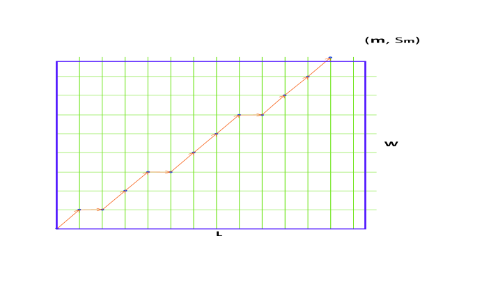
Figure 1: Rectangular Random Walk

Define the relative frequency

$$\widehat{\boldsymbol{p}}=\frac{S_{\boldsymbol{m}}}{\boldsymbol{m}}$$

as an estimator for the desired probability $p$. According to Theorem 2, the mixed criterion (6) is satisfied. We call the above random walk as Rectangular Random Walk as the point with coordinate $(n,S_{n})$ is moving until it is out of the rectangular domain $\mathbb{B}$.

5 Worst-Case Analysis

In this section, we shall investigate the worst-case performance of the method for probability estimation proposed in Section 4. Clearly, the maximum number of simulations is no greater than $L+1$. This is a good thing, since the user can plan the worst requirement of computational resources.

Most importantly, the proposed method is remarkably efficient. Under the assumption that the margin of relative error $\beta$ is small, we can show that the worst-case improvement upon the Chernoff-Hoeffding bound is about a quarter of the ratio of the relative error margin to the absolute error margin, that is,

$$\frac{\text{ Number of simulations by Chernoff-Hoeffding Bound }}{\text{Maximum number of simulations of the proposed method}}\approx\frac{1}{4}\times\frac{\beta}{\alpha}.$$ (7)

As a consequence of the stopping rule for the retangular random walk, the required number of simulations of our method can be much smaller than the worst case bound $L+1$. Hence, the average improvement of our method upon the Chernoff-Hoeffding bound can be much greater than

$$\frac{1}{4}\times\frac{\beta}{\alpha}.$$

To justify the approximate formula (7), we employ Taylor series expansion theory to investigate the ratio

$$\frac{\text{ Number of simulations by Chernoff-Hoeffding Bound }}{\text{Maximum number of simulations of the proposed method}}.$$

Clearly,

$$\frac{\text{ Number of simulations by Chernoff-Hoeffding Bound }}{\text{Maximum number of simulations of the proposed method}}\approx\frac{\frac{\ln\frac{2}{\delta}}{2\alpha^{2}}}{L},$$

where

$$L=\frac{\beta}{(1+\beta)\ln(1+\beta)-\beta}\frac{\ln\frac{2}{\delta}}{\alpha}.$$

Hence,

$$\frac{\text{ Number of simulations by Chernoff-Hoeffding Bound }}{\text{Maximum number of simulations of the proposed method}}\approx\frac{1}{2}\frac{\beta}{\alpha}\times\frac{(1+\beta)\ln(1+\beta)-\beta}{\beta^{2}}.$$

By Taylor series expansion theory, we have

$$\ln(1+x)\approx x-\frac{x^{2}}{2}$$

for small $|x|$. Hence,

$$\frac{(1+\beta)\ln(1+\beta)-\beta}{\beta^{2}}\approx\frac{(1+\beta)(\beta-\frac{\beta^{2}}{2})-\beta}{\beta^{2}}=\frac{1}{2}(1-\beta)\approx\frac{1}{2},$$

which implies (7).

The approximate formula (7) indicates that our proposed method offers an extremely significant advancement in terms of efficiency, without loss of rigorousness. The rationale is that in practices, one can accept a relative margin in orders of magnitude larger than an absolute margin. For example, to estimate the probability $p$ of a critical failure, it is expected to estimate $p$ within an absolute error of $10^{-6}$. The required number of simulations calculated with the Chernoff-Hoeffding bound is $3,800,451,229,772$ for $\delta=10^{-3}$. Even with current super computers, it is unthinkable to perform such an astronomical number of simulations. To overcome such difficulty of computational complexity, we use the mixed criterion proposed in Section 4.1. We consider a very mild relaxation by introducing a requirement of relative error. According to the approximate formula (7), our method can lead to a reduction of computation by a factor of

$$\frac{1}{4}\times\frac{10^{-2}}{10^{-6}}=2,500.$$

Note that an estimate of one percent relative error is an extremely stringent requirement of accuracy. More reduction of computation is possible if the margin of relative error is increased. For example, if the margin of relative error is $0.1$, the computation can be reduced by a factor of

$$\frac{1}{4}\times\frac{10^{-1}}{10^{-6}}=25,000.$$

6 Conclusion

We have developed a general theory of truncated inverse binomial sampling. The theory have been applied to estimate the probability of event. Worst-case analysis shows that the proposed method is extremely efficient as compared to the widely used Chernoff-Hoeffding bound, without scarifying the rigorousness of error control in the estimation of probability of event.

References

- [1]
- [2] G. Agha and K. Palmskog, “A survey of statistical model checking,” ACM Transactions on Modeling and Computer Simulation, vol. 28, pp. 1–39, 2018.
- [3] E. Capello and R. Tempo, “A randomized approach for robust control of uncertain UAVs,” 2nd IFAC Workshop on Research, Education and Development of Unmanned Aerial Systems, pp. 226–231, Compiegne, France, November 2013.
- [4] E. Capello and R. Tempo, “A simulation-based approach for control design of uncertain UAVs,” IEEE Conference on Decision and Control, pp. 3086–3091, December 10-13, 2012. Maui, Hawaii, USA.
- [5] X. Chen, “A theory of truncated inverse sampling,” Sequential Analysis, vol. 37, pp. 455–486, 2019.
- [6] H. Chernoff, “A measure of asymptotic efficiency for tests of a hypothesis based on the sum of observations,” Annals of Mathematical Statistics, vol. 23, pp. 493–507, 1952.
- [7] A. David, K. Larsen, A. Legay, M. Mikucionis, and D. Poulsen, “Uppaal SMC tutorial”, International Journal on Software Tools for Technology Transfer, vol. 17, pp. 397–415, 2015.
- [8] F. Dabbene, C. Lagoa, P. Shcherbakov, and A. Tremba, “RACT - Randomized algorithms control toolbox: A tutorial introduction,” IEEE International Symposium on Intelligent Control, 2008.
- [9] F. Dabbene and R. Tempo,“Randomized methods for control of uncertain systems,” Encyclopedia of Systems and Control, Springer-Valag, 2014.
- [10] F. Dabbene and R. Tempo, “Probabilistic and randomized tools for control design,” The Control System Handbook – Control System Advanced Methods, CRC Press, Second Edition, 2011.
- [11] M. M. Desu and D. Raghavarao, Sample Size Methodology, Academic Press, 1990.
- [12] G. S. Fishman, Monte Carlo: Concepts, Algorithms, and Applications, Springer, 2003.
- [13] F. Hampel, “Is statistics too difficult?” The Canadian Journal of Statistics, vol. 26, pp. 497-513, 1998.
- [14] T. Hrault, S. Peyronnet, and R. Lassaigne, “APMC 3.0: Approximate verification of discrete and continuous time Markov chains,” Proceedings of International Conference on Quantitative Evaluation of Systems, pp. 129–130, Riverside, California, 2006.
- [15] W. Hoeffding, “Probability inequalities for sums of bounded random variables,” Journal of the American Statistical Association, vol. 58, pp. 13–30, 1963.
- [16] M. Kwiatkowska, G. Norman, and D. Parker, “PRISM 4.0: Verification of probabilistic real-time systems,” Lecture Notes in Computer Science, vol. 6806, pp. 585–591, Springer, 2011.
- [17] A. Legay, B. Delahaye, and S. Bensalem, “Statistical model checking: An overview,” Lecture Notes in Computer Science, vol. 6418, Springer, Berlin, 2010.
- [18] T. Mitchell, Machine Learning, Mc Graw Hill, 1997.
- [19] M. Mitzenmacher and E. Upfal, Probability and Computing: Randomized Algorithms and Probabilistic Analysis, Cambridge University Press, Second edition, 2017.
- [20] R. Motwani and P. Raghavan, Randomized Algorithms, Cambridge University Press, 1995.
- [21] R. Tempo, G. Calafiore, and F. Dabbene, Randomized Algorithms for Analysis and Control of Uncertain Systems: With Applications, Second edition, Springer, 2013.
- [22] A. Tremba, G. Calafiore, F. Dabbene, E. Gryazina, B. Polyak, P. Shcherbakov, and R. Tempo, “RACT: Randomized algorithms control toolbox for MATLAB,” Proceedings of the 17th World Congress of The International Federation of Automatic Control, pp. 390–395, Seoul, Korea, July 2008.
- [23] V. N. Vapnik, The Nature of Statistical Learning, Springer, 1995.
- [24] V. N. Vapnik, Statistical Learning Theory, Wiley, 1998.
- [25] M. Vidyasagar, Learning and Generalisation: With Applications to Neural Networks, Springer, 2nd ed., 2002.
- [26] H. L. S. Younes, “Error control for probabilistic model checking,” Proceedings of International Workshop on Verification, Model Checking, and Abstract Interpretation, pp. 142–156, 2006.