A persistent homology approach to heart rate variability analysis with an application to sleep-wake classification

Abstract.

Persistent homology (PH) is a recently developed theory in the field of algebraic topology to study shapes of datasets. It is an effective data analysis tool that is robust to noise and has been widely applied. We demonstrate a general pipeline to apply PH to study time series; particularly the instantaneous heart rate time series for the heart rate variability (HRV) analysis. The first step is capturing the shapes of time series from two different aspects – the PH’s and hence persistence diagrams of its sub-level set and Taken’s lag map. Second, we propose a systematic and computationally efficient approach to summarize persistence diagrams, which we coined persistence statistics. To demonstrate our proposed method, we apply these tools to the HRV analysis and the sleep-wake, REM-NREM (rapid eyeball movement and non rapid eyeball movement) and sleep-REM-NREM classification problems. The proposed algorithm is evaluated on three different datasets via the cross-database validation scheme. The performance of our approach is better than the state-of-the-art algorithms, and the result is consistent throughout different datasets.

1. Introduction

Heart rate variability (HRV) is the physiological phenomenon of variation in the lengths of consecutive cardiac cycles, or the rhythm of heart rate [29]. Interest in HRV has a long history [11], and there have been several theories describing how the heart rate rhythm, including, for example, the polyvagal theory [62] and the model of neurovisceral integration [72]. In short, HRV results from an integration of complicated interactions between various physiological systems and external stimuli [76, 29, 65] on various scales, and the autonomic nervous system (ANS) plays a critical role [62, 72]. A correct quantification of HRV yields dynamical information of various physiological systems and has various clinical applications [69], including improving diagnostic accuracy and treatment quality [76].

In practice, the heart rhythm is quantified by the time series called instantaneous heart rate (IHR) coming from intervals between consecutive pairs of heart beats, which is usually determined from the R peak to R peak interval (RRI) by reading the electrocardiogram (ECG). To quantify HRV, a common approach is studying various statistics of IHR. There have been a lot of efforts trying to quantify HRV, and proposed statistics could be briefly classified into four major categories – time domain approach, frequency domain approach [71], nonlinear geometric approach [80, 51], and information theory based approach [27]. It is worth mentioning that while there have been a lot of researches in this direction with several proposed statistics, there is limited consensus and it is still an active research field due to the non-stationarity nature of the IHR time series [61, 37].

Topological data analysis (TDA) is a data analysis framework based on tools from algebraic topology [34, 16]. In the past decades, its theoretical foundation has been actively established, and various algorithms have been proposed to study datasets from different fields. The basic idea underlying TDA is that the data organization can be well captured by counting holes. Theoretically, the number of holes of different dimensions characterizes how the data is organized. Thus, researchers design useful statistics based on the information of holes. This simple yet powerful idea has been applied to different fields. Specifically, there have been several efforts applying TDA to analyze time series. For example, the Vietoris-Rips (VR) complex filtration and the bottleneck or Wasserstein distances among persistence diagrams (PDs) are applied to study voices and body motions [64, 78]. A transformation of the PD, called persistence landscapes [15], has been applied to study trading records [36], EEG signals [81] and cryptocurrency trend forecasting [46]. However, to the best of our knowledge, its application to HRV is not yet considered. Moreover, existing TDA approaches usually suffer from computational issues, which limits its application to large scale database. Finding a computationally efficient TDA algorithm is thus critical.

In this article, motivated by the complicated interaction among different physiological systems over various scales and inter-individual variability, the need for a useful tool for the HRV analysis, and the numerical limitation of the recently developed TDA tools, we hypothesize that topological information could be useful to quantify the HRV, and propose a computationally efficient approach to analyze time series via TDA.

1.1. Our contribution

Based on the flexibility of TDA tools, and due to the non-stationarity of complicated time series we commonly encounter in real life, like the IHR, we propose a systematic, principled, and computationally efficient approach to study complicated time series by the TDA tools.

Our main scheme for studying a complicated time series is shown in Fig. 1, which is divided into three steps that we will detail later. First, consider two filtrations, the Vietoris-Rips (VR) complex filtration of the Takens’ lag map [70] and the sub-level set filtration of the time series, and persistent homology (PH). Second, compute corresponding PDs. Finally, calculate persistence statistics (PS) as a novel statistic of the time series of interest. We mention that compared with existing TDA approach for time series analysis, our proposed PS features based on both sub-level set and VR complexes filtrations are intuitive, straightforward to implement, and also computationally efficient.

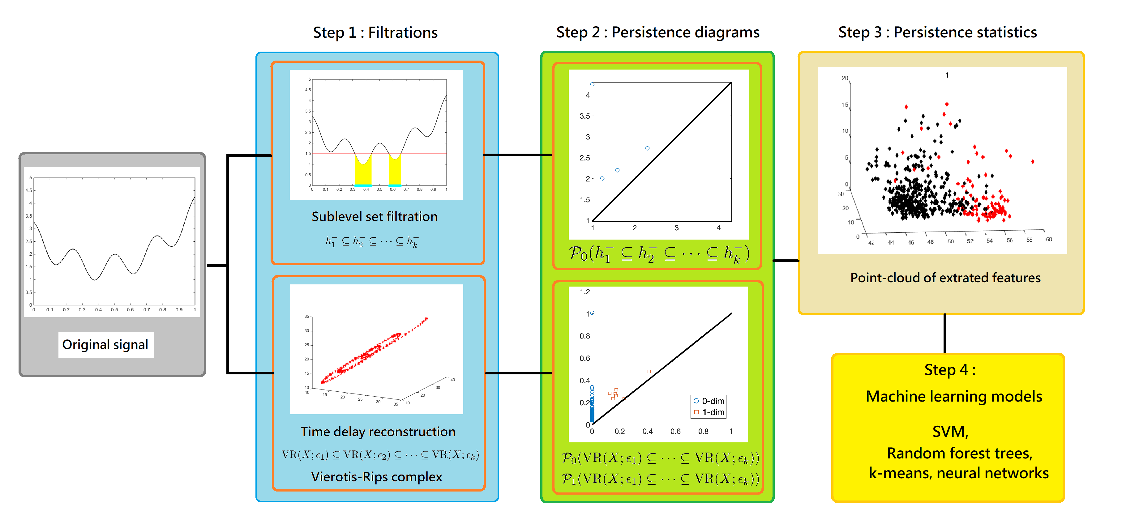
Figure 1. The scheme of our proposed time series analysis can be separated by three steps: constructing filtrations, computing PD’s and extracting PS as features. The features are applied to train a machine learning model for the classification purpose.

1.2. Application – Sleep dynamics

To demonstrate the usefulness of the proposed PS, we apply it to study IHR time series recorded during sleep, and use obtained statistics to classify sleep stages. Sleep is a universal recurrent physiological phenomenon. Sleep impacts the whole body, so we can read sleep via reading different physiological signals. Taking ECG into account is specifically attractive, since the ECG sensor is easy to install, and it is now widely available in mobile health devices. HRV of a subject is usually quantified by analyzing ECG, and it has been shown to be related to sleep dynamics [84, 77, 73, 14, 33, 21, 60]. In other words, the heart rate rhythm provides a non-invasive window for researchers to study sleep. While there have been several studies trying to classify sleep stages based on HRV [48, 52, 49, 82, 3, 83, 50], it still remains a challenging problem in the field. The challenge and difficulty of this mission can be appreciated from the reported results. In this article, we apply the proposed PS to quantify HRV during sleep, and propose a new prediction algorithm for the sleep stage; for example, an automatic classification of wake and sleep, REM and NREM, and wake, REM and NREM. We remark that while we focus on the HRV and sleep stage classification, the result indicates the potential of applying TDA-based approaches to study other complicated time series.

1.3. Organization

In Section 2, we review the mathematical background of the PH and PD. In Section 3, we demonstrate two ways to use the PH to study time series, and propose a new approach to summarize the PD, called the PS. The classification model based on the PS for the sleep stage classification will be discussed in detail in Section 4. The discussion of our classification performance and a comparison with the state-of-arts results will be included in Section 5. More technical details and numerical results are postponed to the Online Supplementary.

2. Mathematical Background

In this section, we describe the mathematical background, including simplicial complex, homology, filtration of sets and the PH. Although these topics can be studied in an abstract and general way (see e.g. [56]), to enhance the readability, we present them in a relatively concrete way without losing critical information.

2.1. Simplicial Complexes

To investigate the complicated structure of an object, an intuitive way is to use simple objects as building blocks to approximate the original object. In TDA, the main building block is the simplicial complex, which we briefly recall now. See Section SI.1.1 for more detailed mathematical background and illustrative examples.

We start with the simplex. Intuitively, a simplex is a “triangle” of different dimension. Let $x_{0},x_{1},\ldots,x_{q}$ be affinely independent points in $\mathbb{R}^{d}$, where $d,q\in\mathbb{N}$ and $d\geq q$. The $q$-simplex, denoted by $\sigma:=\langle x_{0},x_{1},\ldots,x_{q}\rangle$, is defined to be the convex hull of $x_{0},x_{1},\ldots,x_{q}$. Denote ${\rm Vert}(\sigma):=\{x_{0},x_{1},\ldots,x_{q}\}$. Any $q$-simplex is a $q$-dimensional object consisting of lower degree simplexes. We are interested in the relation among simplexes of different dimensions. Since any $V\subset{\rm Vert}(\sigma)$ is also affinely independent, the convex hull of $V$, called a face of $\sigma$, forms a simplex of dimension $|V|\leq q$, where $|V|$ is the cardinality of $V$. If $|V|=k$, the face $\tau=\langle V\rangle$ is called a $k$-face of $\sigma$. A simplicial complex $\mathcal{K}$ in $\mathbb{R}^{d}$ is a collection of finite simplexes $\sigma$ in $\mathbb{R}^{d}$ so that any intersection of two arbitrary simplexes is a face to each of them; that is,

• If $\sigma\in\mathcal{K}$ and $\tau$ is a face of $\sigma$, then $\tau\in\mathcal{K}$;

• If $\sigma_{1},\sigma_{2}\in\mathcal{K}$, then $\sigma_{1}\cap\sigma_{2}$ is a face of $\sigma_{1}$ and $\sigma_{2}$. In particular, $\sigma_{1}\cap\sigma_{2}\in\mathcal{K}$.

2.2. Homology and Betti numbers

In order to study the topological information of a given simplicial complex, we study relations among simplexes of different dimensions, and hence the “holes”. Homology and Betti numbers are classic subjects in the algebraic topology [56], which capture “holes” of geometric objects of different dimensions. While we can discuss these topics in a more general setup, in this work, we mainly consider simplicial complexes as our target object. See Section SI.1.2 for more information and illustrative examples.

We need an algebraic structure of simplexes. Given $q$-simplexes $\sigma_{1},\sigma_{2},\ldots,\sigma_{n}$ in a simplicial complex $\mathcal{K}$, define the sum over $\mathbb{Z}_{2}$ as $c=\sum_{i=1}^{n}\nu_{i}\sigma_{i}$, where $\nu_{i}\in\mathbb{Z}_{2}$. This formal sum is commonly known as a $q$-chain. One could also define an addition operator as $\sum_{i=1}^{n}\nu_{i}\sigma_{i}+\sum_{i=1}^{n}\mu_{i}\sigma_{i}:=\sum_{i=1}^{n}(\nu_{i}+\mu_{i})\sigma_{i}$. We consider the collection of all $q$-chains, denoted as

(1) $$C_{q}(\mathcal{K}):=\bigg{\{}\sum_{i=1}^{n}\nu_{i}\sigma_{i}~{}\Big{|}~{}\nu_{i}\in\mathbb{Z}_{2},~{}\sigma_{i}\in\mathcal{K},~{}\dim(\sigma_{i})=q\bigg{\}}.$$

One could prove that $C_{q}(\mathcal{K})$ is actually a vector space over $\mathbb{Z}_{2}$ with the above addition. There is a natural relation between $C_{q}(\mathcal{K})$ and $C_{q-1}(\mathcal{K})$, called the boundary map [56, Sec. 1.5, p. 30]. The $q^{\rm th}$ boundary map $\partial_{q}:C_{q}(\mathcal{K})\rightarrow C_{q-1}(\mathcal{K})$ over $\mathbb{Z}_{2}$ is defined by

(2) $$\partial_{q}(\langle x_{0},x_{1},\cdots,x_{q}\rangle):=\sum_{i=0}^{q}\langle x_{0},\cdots,\widehat{x_{i}},\cdots x_{q}\rangle,$$

where $\langle x_{0},x_{1},\cdots,x_{q}\rangle\in\mathcal{K}$ and the $\widehat{\bullet}$ denotes the drop-out operation. With the boundary maps, there is a nested relation among chains

(3) $$\cdots\xrightarrow[]{\partial_{n+1}}C_{n}(\mathcal{K})\xrightarrow[]{\partial_{n}}C_{n-1}(\mathcal{K})\xrightarrow[]{\partial_{n-1}}\cdots C_{1}(\mathcal{K})\xrightarrow[]{\partial_{1}}C_{0}(\mathcal{K}).$$

This nested relation among chains is known as the chain complex, which is denoted as $\mathcal{C}=\{C_{q},\partial_{q}\}_{q\in\mathbb{Z}}$.

A fundamental result in the homology theory ([56] Lemma 5.3 Sec. 1.5, p. 30) is that the composition of any two consecutive boundary maps is trivial, i.e. $\partial_{q-1}\circ\partial_{q}=0$. This result allows one to define the following quotient space. Denote cycles and boundaries by $Z_{q}$ and $B_{q}$, respectively, which are defined as

$$Z_{q} :=\ker(\partial_{q})=\{c\in C_{q}\ |\ \partial_{q}(c)=0\},\,B_{q}:={\rm im}(\partial_{q+1})=\{\partial_{q+1}(z)\in C_{q}\ |\ z\in C_{q+1}\}.$$

Note that each $B_{q}$ is a subspace of $Z_{q}$ since $\partial_{q-1}\circ\partial_{q}=0$. Therefore, we can define the $q^{\rm th}$ homology to be the quotient space

(4) $$H_{q}(\mathcal{K}):=\frac{Z_{q}}{B_{q}}=\frac{\ker(\partial_{q})}{{\rm im}(\partial_{q+1})},$$

which is again a vector space. The $q^{\rm th}$ Betti number is defined to be the dimension of the $q^{\rm th}$ homology; that is,

(5) $$\beta_{q}(\mathcal{K})=\dim(H_{q}(\mathcal{K}))\,,$$

which measures the number of $q$-dimensional holes. As a result, given a simplicial complex $\mathcal{K}$, the homology of $\mathcal{K}$ is a collection of vector spaces $\{H_{q}(\mathcal{K})\}_{q=0}^{\infty}$, and its Betti numbers is denoted as $\beta(\mathcal{K}):=\{\beta_{q}(\mathcal{K})\}_{q=0}^{\infty}$.

2.3. Persistent Homology

We now introduce a natural generalization of homology, the PH, that is suitable for data analysis. PH is more suitable for data analysis than homology due to this capability of dealing with inevitable noise in real world dataset. It depends on the notion of filtration to handle noise. In general, filtration is a sequence of simplicial complexes (see Fig. 2 for an example). We are interested in how the “holes” vary in the filtration. Intuitively, if certain holes are “robust”, they will survive in the filtration.

Definition 1 ([30] Sec. III.4, p. 70).

For an index set $I$, a filtration is a sequence of simplicial complexes, $\{\mathcal{K}_{t}\}_{t\in I}$, satisfying

(6) $$\mathcal{K}_{t_{1}}\subseteq\mathcal{K}_{t_{2}},\text{ whenever }t_{1}\leq t_{2}.$$

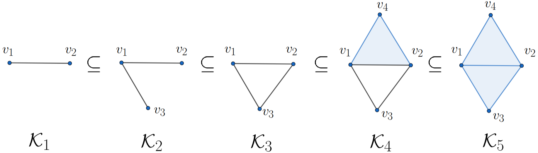
Figure 2. Illustration of a filtration of simplicial complexes $\mathcal{K}_{1},\mathcal{K}_{2},\mathcal{K}_{3},\mathcal{K}_{4}$ and $\mathcal{K}_{5}$.

From the previous discussion, for each $\mathcal{K}_{t}$ in a filtration, one could compute its homology group and Betti number. Because of the nested subset relation in a filtration, there exist relations among simplicial complexes. This allows one to track and record the changes of the homology group and the Betti numbers, which we detail now. Given a fixed $q\geq 0$, each $\mathcal{K}_{i}$ induces homology $H_{q}(\mathcal{K}_{i})$. Denote $\iota_{i}:\mathcal{K}_{i}\rightarrow\mathcal{K}_{i+1}$ to be the inclusion map. Then $\iota_{i}(Z_{q}(\mathcal{K}_{i}))\subseteq Z_{q}(\mathcal{K}_{i+1})$ and $\iota_{i}(B_{q}(\mathcal{K}_{i}))\subseteq B_{q}(\mathcal{K}_{i+1})$ ([30] Sec. IV.4, p. 95). Therefore, the mapping

(7) $$\iota_{i,H_{q}}:H_{q}(\mathcal{K}_{i})\rightarrow H_{q}(\mathcal{K}_{i+1}),\ \ \overline{c}\longmapsto\overline{\iota_{i}(c)}$$

induced by $\iota_{i}$ is a well-defined linear transformation over $\mathbb{Z}_{2}$. We also define a linear transformation

(8) $$\rho_{q}^{i,i+k}:=\iota_{i+k-1,H_{q}}\circ\cdots\circ\iota_{i+1,H_{q}}\circ\iota_{i,H_{q}},$$

which maps $H_{q}(\mathcal{K}_{i})$ to $H_{q}(\mathcal{K}_{i+k})$. The following definition is crucial for defining lifespans of connected components or holes in homology theory.

Definition 2 ([30] Sec. VII.1, p. 151).

Let $\{\mathcal{K}_{i}\}_{i=0}^{n}$ be a filtration of simplicial complexes. For $q\in\mathbb{Z}_{\geq 0}$ and $i,j\in\mathbb{Z}_{\geq 0}$ with $i\leq j$, we define the PH as

(9) $$\ H_{q}^{i,j}:=\frac{Z_{q}(\mathcal{K}_{i})}{B_{q}(\mathcal{K}_{j})\cap Z_{q}(\mathcal{K}_{i})}.$$

Since $\mathcal{K}_{0}\subseteq\mathcal{K}_{1}\subseteq\cdots\subseteq\mathcal{K}_{n}$, we have inclusions of $q$-chains: $C_{q}(\mathcal{K}_{0})\subseteq C_{q}(\mathcal{K}_{1})\subseteq\cdots\subseteq C_{q}(\mathcal{K}_{n})$ for all $q\geq 0$. Hence, the intersection $B_{q}(K_{j})\cap Z_{q}(\mathcal{K}_{i})$ is a well-defined subspace of $Z_{q}(\mathcal{K}_{i})$. Moreover, for $i\leq j$, the kernel of the linear transformation

$$\phi:Z_{q}(\mathcal{K}_{i})\longrightarrow\frac{Z_{q}(\mathcal{K}_{j})}{B_{q}(\mathcal{K}_{j})},\ \ c\longmapsto\overline{c}=c+B_{q}(\mathcal{K}_{j})$$

induced by the inclusion map is $B_{q}(\mathcal{K}_{j})\cap Z_{q}(\mathcal{K}_{i})$. By the first isomorphism theorem, we obtain an injective linear transformation

$$\overline{\phi}:\frac{Z_{q}(\mathcal{K}_{i})}{B_{q}(\mathcal{K}_{j})\cap Z_{q}(\mathcal{K}_{i})}\longrightarrow\frac{Z_{q}(\mathcal{K}_{j})}{B_{q}(\mathcal{K}_{j})}\,.$$

Via the one-to-one linear mapping $\overline{\phi}$, the vector space $H_{q}^{i,j}$ may be viewed as a subspace of $H_{q}(\mathcal{K}_{j})$. In particular, if $i=j$, then $H_{q}^{i,j}=H_{q}(\mathcal{K}_{i})=H_{q}(\mathcal{K}_{j})$, which means that the PH is a generalization of the homology. With the inclusion $H_{q}^{i,j}\hookrightarrow H_{q}(\mathcal{K}_{j})$, we define the moments of birth and death of a “hole” in the filtration.

Definition 3 ([30] Sec. VII.1, p. 151).

Let $\{\mathcal{K}_{i}\}_{i=0}^{n}$ be a filtration of simplicial complexes and $q\in\mathbb{Z}_{\geq 0}$.

• A $q$-th class $\overline{c}$ ($c\in Z_{q}(\mathcal{K}_{i})$) is born at $\mathcal{K}_{i}$ if $\overline{c}\in H_{q}(\mathcal{K}_{i})\setminus\{0\}$, but $\overline{c}\notin{\rm{\rm im}}(\rho_{q}^{i-1,i})$;

• A $q$-th class $\overline{c}$ ($c\in Z_{q}(\mathcal{K}_{i})$) dies at $\mathcal{K}_{j}$ if $\rho_{q}^{i,j-1}(\overline{c})\notin H_{q}^{i-1,j-1}$, but $\rho_{q}^{i,j}(\overline{c})\in H_{q}^{i-1,j}$.

We use Fig. 2 to explain the relation between these two abstract definitions. For instance, the non-trivial class $\overline{c}$ represented by $1$-chain

$$\begin{split}c&=\langle v_{1},v_{2}\rangle+\langle v_{2},v_{3}\rangle+\langle v_{3},v_{1}\rangle\end{split}$$

in $H_{1}(\mathcal{K}_{3})$ is born at $\mathcal{K}_{3}$ i.e. $\overline{c}\notin{\rm im}(\rho_{1}^{2,3})$ because $H_{1}(\mathcal{K}_{2})=\{0\}$ and $\mathbb{Z}_{2}=H_{1}(\mathcal{K}_{3})=\langle\overline{c}\rangle$. On the other hand, the fact $\{0\}\subseteq H_{1}^{2,5}\subseteq H_{1}(\mathcal{K}_{5})=\{0\}$ shows that $\rho_{1}^{3,5}(\overline{c})\in H_{1}(\mathcal{K}_{5})=H_{1}^{2,5}$ and $\rho_{1}^{3,4}(\overline{c})\notin H_{1}^{2,4}$ because $H_{1}^{2,4}=\{0\}$ (since $Z_{1}(\mathcal{K}_{2})=\{0\}$) and $\mathbb{Z}_{2}=H_{1}(\mathcal{K}_{4})=\langle\rho_{1}^{3,4}(\overline{c})\rangle$, thus $\overline{c}$ dies at $\mathcal{K}_{5}$. We refer readers with interest to [30] for more details in PH.

2.4. Persistence Diagram

Persistence diagram (PD) proposed in [31] or equivalently persistence barcodes proposed in [17] is a tool to visualize the complicated lifespans of holes in a given filtration for data analysis. We use PD in this paper.

The PD possesses the desired stability property [24] – a bounded perturbation of a given filtration leads to a bounded perturbation of the corresponding PD. Due to the inevitable noise in real data, this stability property renders PD-based approaches suitable for data analysis. The bottleneck and Wasserstein distances [24] are typical ways to measure differences among PDs. The formal statements of the stability property based on these two distances are provided in Section 3.1 and Section 3.2. We refer readers with interest to [30] for details in PD.

Definition 4 ([30] Sec. VII.1, p. 152).

Let $\{\mathcal{K}_{i}\}_{i=0}^{n}$ be a filtration of simplicial complexes and $q\in\mathbb{Z}_{\geq 0}$. The $q^{\text{th}}$ PD, denoted as $\mathcal{P}_{q}(\{\mathcal{K}_{i}\}_{i=0}^{n})$, of the filtration is the multiset of $q$-dimension holes in the filtration. More precisely, $\mathcal{P}_{q}(\{\mathcal{K}_{i}\}_{i=0}^{n})$ is the multiset of all tuples $(b,d)$ corresponding to $q$-dimensional holes $\overline{c}$ which satisfy $\rho_{q}^{b,d-1}(\overline{c})\notin H_{q}^{b-1,d-1}$ and $\rho_{q}^{b,d}(\overline{c})\in H_{q}^{b-1,d}$.

In other words, a $q$-dimensional hole in a filtration is recorded by a pair $(b,d)$ of integers where $b$ and $d$ are called the birth and death of the hole respectively [30]. Although the above definition of PD seems technical, its interpretation is intuitive. For instance, consider the filtration shown in Fig. 2. We look for the “changes” of topological structure (holes). Note that since a connected component is born at $\mathcal{K}_{1}$ (specifically, $\langle v_{1},v_{2}\rangle$), its birth value is $b=1$; since it lives throughout the filtration, its death value is $\infty$. We now turn our focus to the 1-dimensional hole. Note that a 1-dimensional hole (specifically, $\langle v_{1},v_{2}\rangle+\langle v_{2},v_{3}\rangle+\langle v_{1},v_{3}\rangle$) is formed at $\mathcal{K}_{3}$, so its birth value is $3$; note also that this hole is filled at $\mathcal{K}_{5}$, so its death value is $5$. Since there is no more change of holes, we have the persistence diagrams $\mathcal{P}_{0}(\{\mathcal{K}_{i}\}_{i=1}^{5})=\{(1,\infty)\}$ and $\mathcal{P}_{1}(\{\mathcal{K}_{i}\}_{i=1}^{5})=\{(3,5)\}$.

Before closing this subsection, we illustrate how PH and PD work by taking a noisy point cloud sampled from a circle contaminated by Gaussian noise shown in Fig. 3(a). If there is no noise, the 1st Betti number of the circle is $\beta_{1}=1$. In the noisy case, the Betti number information is contained in the form of the PD as shown in Fig. 3(b), where each point represents one 1-dimensional hole associated with its birth and death value. In Fig. 3(b), we observe that there is an outstanding point with long lifespan (located around birth value 0.05 and death value 0.25), while lifespans for other points are very small. This suggests that the noisy point cloud has a strong/robust 1-dimensional hole. This captures the main topology information, $\beta_{1}=1$, about this data.

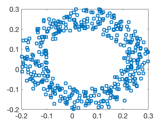
(a) Point cloud data $X$.

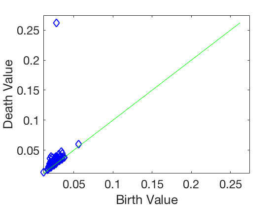
(b) $\mathcal{P}_{1}(X)$.

Figure 3. Toy example of the persistent homology. (a) Data points are sampled from a circle with the Gaussian noise. (b) 1st dimensional persistence diagram.

2.5. Data analysis with PD and commonly considered TDA statistics

Usually, researchers design statistics on the PD of a given dataset via the chosen filtration. One basic result supporting this approach is [53], where authors showed that the space of PDs with certain metric is complete and separable. This result forms a theoretic foundation for any statistical methods. In [35, 12], authors derived confidence sets of PDs in order to separate the long lifespan holes from noisy ones, and also proposed four ways to estimated them. While these theoretical results shed light on applying TDA to analyze complex data, however, any operation in the space of PDs is complicated and difficult to compute. For example, computing bottleneck or Wasserstein distances among PDs is a difficult task and can be time consuming, even for the state-of-art algorithm [45]. Another result indicates that the mean in the space of PDs may not be unique [74]. This computational burden renders it less applicable to data analysis.

To get around the computational issue when working with those distances, one major approach is to “vectorize” PDs; that is, researchers map the space of PDs into another space. For example, persistence landscapes [15] map PDs into a Banach space, specifically $L^{p}$ space. More examples include persistence image [1], generalized persistence landscapes [8], persistence path [19], persistence codebook [85], persistence curves [23], kernel based methods [63, 47], and persistent entropy [5, 20]. These methods have been studied and applied to different applications. In Fig. 4, we provide a chart depicting the relationship among existing TDA tools. We mention that the proposed PS in Section 3 could be viewed as a computationally efficient vectorization of PD’s.

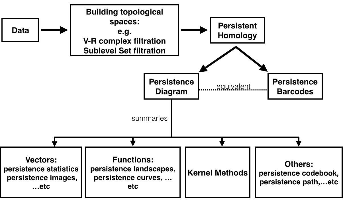
Figure 4. A chart depicting relationship among existing TDA tools.

3. TDA for time series analysis and features extraction

Armed with the theoretical background in Section 2, we are ready to describe how to apply TDA for time series analysis. To apply the PH to analyze complicated time series, we introduce two useful filtrations, the sub-level set filtration and the VR complexes filtration. With these two filtrations, we introduce a novel features extraction methods, coined PS, based on the PDs of the sub-level set filtration and the VR complexes filtration.

3.1. First useful filtration – Sub-level set Filtration

To simplify the discussion and illustrate the idea, we identify a time series as a discretization of a continuous function $f:[0,T]\rightarrow\mathbb{R}$, where $T$ is some fixed constant. For each $h\in\mathbb{R}$, the sub-level set of $f$ is defined as

(10) $$f_{h}:=f^{-1}((-\infty,h])=\{t\in[0,T]\ |\ f(t)\leq h\}.$$

Clearly, $f_{h_{1}}\subseteq f_{h_{2}}$ whenever $h_{1}\leq h_{2}$. Therefore, for any increasing sequence $\{h_{i}\}_{i}$, the collection of sub-level sets, $\{f_{h_{i}}\}$, forms a filtration. Intuitively, the sub-level set filtration reveals the oscillating information of the functions. Since each $f_{h}$ is a subset of $[0,T]\subseteq\mathbb{R}$, it only contains $0$-dimensional structures, i.e., connected components. Hence, the only non-trivial PD in this case is $\mathcal{P}_{0}$. For simplicity, when there is no danger of confusion, for a given function $f$, we use $\mathcal{P}_{0}(f)$ to denote $\mathcal{P}_{0}(\{f\}_{h_{i}})$, the PD associated with the sub-level sets filtration of $f$. As discussed in [30], each element in $\mathcal{P}_{0}$ is a min-max pair in the original function $f(t)$. The concept of this filtration is closely related to the size function theory (see [10] and references therein) and is commonly used as a shape descriptor [10]. In practice, PD is robust to noise under the bottleneck distance. This fact renders PD an useful data analysis quantity. A precise statement of this robustness is below.

Theorem 3.1.1.

Let $X$ be an $n$-dimensional rectangle in $\mathbb{R}^{n}$. Take two continuous functions $f,g:X\rightarrow\mathbb{R}$ with finitely many local extremums (minimums or maximums). Then, we have for $q\in\mathbb{N}$,

$$d_{B}(\mathcal{P}_{q}(f),\mathcal{P}_{q}(g))\leq\|f-g\|_{\infty},$$

where $d_{B}$ is the bottleneck distance defined as $d_{B}(M,N)=\inf_{\gamma}\sup_{m\in M}\|m-\gamma(m)\|_{\infty}$, where $\gamma$ ranges over all bijections from multisets $M$ to $N$. Here we interpret each point with multiplicity $k$ as $k$ individual points and the bijection is between the resulting sets.

In fact, Theorem 3.1.1 is a special form of a stability theorem (Main Theorem in [24], p. 109). See Section SI.1.3 for an illustrative example of the sub-level sets filtration.

3.2. Second useful filtration – Vietoris-Rips Complexes Filtration

To introduce Vietoris-Rips (VR) complexes filtration for a given time series, we first embed the time series into a high dimension point cloud via Taken’s lag map [70], which is constructed in the following way. Take $p\in\mathbb{N}$ to be the dimension of the embedding, and $\tau\in\mathbb{N}$ to be the lag step. For a given time series $H:\mathbb{Z}\to\mathbb{R}$, the lag map with lag $\tau$ and dimension $p$ is defined as

(11) $$R_{p,\tau}(H)=\{(H(t),H(t-\tau),H(t-2\tau),\ldots,H(t-(p-1)\tau))^{\top}|\,t\in\mathbb{Z}\}\,,$$

which is a subset of $\mathbb{R}^{p}$. We postpone details of Taken’s lag map to Section SI.2. With the point cloud $R_{p,\tau}\subset\mathbb{R}^{p}$, we are ready to introduce the VR complex.

In general, given a point cloud $\mathcal{X}=\{x_{1},\ldots,x_{N}\}\subset\mathbb{R}^{p}$, the main idea of VR complex is to build simplicial complexes from $\mathcal{X}$ if points in $\mathcal{X}$ are closed enough. A formal definition is given below.

Definition 5 ([30] Sec. III.2, p. 61).

Let $X=\{x_{1},x_{2},\ldots,x_{N}\}\subseteq\mathbb{R}^{p}$ be a point cloud and take $\epsilon>0$. The VR complex is a collection of all $q$-simplexes $\sigma$ with vertices in $X$ with ${\rm diam}(\sigma)\leq 2\epsilon$, where ${\rm diam}(\sigma)$ is the diameter of $\sigma$; that is,

(12) $${\rm VR}(X;\epsilon):=\bigcup_{q=0}^{p}\left\{q{\rm-simplex}\ \sigma\ |\ {\rm diam}(\sigma)\leq 2\epsilon,{\rm Vert}(\sigma)\subseteq X\right\}.$$

Clearly, for an increasing sequence $\epsilon_{1}<\epsilon_{2}<\cdots<\epsilon_{N}$, the corresponding sequence of VR complexes forms a filtration:

(13) $${\rm VR}(X;\epsilon_{1})\subseteq{\rm VR}(X;\epsilon_{2})\subseteq\cdots\subseteq{\rm VR}(X;\epsilon_{N}).$$

After determining the representation rules of connected components, the lifespan of holes of different dimensions can be computed easily. See Section SI.1.3 for an illustrative example of the VR filtration.

For simplicity, we denote the $q$-th PD associated the VR filtration as $\mathcal{P}_{q}(R_{p,\tau}):=\mathcal{P}_{q}(\{{\rm VR}(R_{p,\tau};~{}\epsilon)\}_{\epsilon})$. In parallel with Theorem 3.1.1, the stability of PDs extracted from a VR filtration has been discussed in [18].

Theorem 3.2.1 ([18], Theorem 5.2).

For finite metric spaces $(X,d_{X})$ and $(Y,d_{Y})$, then for $q\in\mathbb{N}$,

$$d_{B}(\mathcal{P}_{q}({\rm VR}(X)),\mathcal{P}_{q}({\rm VR}(Y)))\leq 2d_{GH}(X,Y),$$

where $d_{B}$ is the bottleneck distance and $d_{GH}$ is the Gromov-Hausdorff distance.

3.3. Persistence Statistics

We now introduce a set of new features to represent PDs. It is computationally efficient and straightforward to implement. Motivated by features considered in [22] to classify different types of skin lesions, and those considered in [55] to study bifurcations and chaos in complex dynamic systems, we propose to explore distributions of the birth $b$ and the death $d$ of all possible holes. To be more specific, given a PD $\mathcal{P}$, we transform it into two multi-sets of numbers, $M$ and $L$, defined as

(14) $$M=\left\{\frac{d+b}{2}~{}\Big{|}~{}(b,d)\in\mathcal{P}\right\}\text{ and }L=\left\{d-b~{}\Big{|}~{}(b,d)\in\mathcal{P}\right\}\,.$$

Note that for the VR complex filtration, $\frac{d+b}{2}$ captures the “size” of the associated hole, and $d-b$ captures the robustness of the associated hole. On the other hand, for the sublevel set filtration, $\frac{d+b}{2}$ reveals the locations of holes, and $d-b$ captures the differences between low and high peaks in a time series. Note that since the hole $(0,\infty)$ always exists in the PD as is shown in the previous section, it is omitted.

In this paper, for each persistence diagram, we consider eight summary statistics to represent the multi-set $M$, including mean, standard deviation, skewness, kurtosis, 25th, 50th, 75th percentile and the persistent entropy [20]. We number them from $1$ to $8$. We consider the same summary statistics for the multi-set $L$, and number them from $9$ to $16$.

Definition 6 (Persistence Statistics).

Given a PD, the PS is defined as a map, $\Phi^{(\texttt{PS})}$, that transforms the PD to $\mathbb{R}^{16}$.

The persistent entropy of $L$ and $M$, denoted as $E(L)$ and $E(M)$ respectively, describes the complexity of $L$ and $M$. It has been used to study the cell arrangements [4] and emotion recognition [39]. From the theoretical perspective, it has been shown that the $E(L)$ is a stability measurement [6]. On the other hand, $E(M)$ is the new quantity that we propose. It would be interesting to investigate theoretic properties of $E(M)$ for the future work.

Note that while intuitively, holes with long lifespans are considered important features and those with short lifespans are considered noises, in our proposed features, we do not discriminate holes with long or short lifespans. In other words, we take all holes into consideration. This approach is supported by a recent discovery that those considered as noisy holes might actually contain important information. For example, in the drivers’ behavior classification [7], authors transformed the space of PDs into “binned” diagrams, and found that the main differences occurred in those short lifespan holes. Another work on the leave classification [59] also suggested that holes with short lifespans could better distinguish different types of leaves.

4. Application to sleep stage classification

In recent decades, a growing body of evidence shows that sleep is not only intimately related to personal health [44, 43] but also has a direct impact on public health [26]. In clinics, sleep experts score sleep stage by reading the electroencephalogram (EEG), electrooculogram (EOG) and electromyogram (EMG) based on the American Academy of Sleep Medicine (AASM) criteria [41, 9]. Sleep, however, impacts the whole body, and we can read sleep via reading physiological signals other than EEG, particularly ECG and HRV mentioned in Introduction. The relationship between HRV and sleep dynamics has been widely studied in the physiology society [84, 77, 73, 14, 33, 21, 60]. Specifically, when a subject is awake, since the sympathetic tone of the ANS is dominant, he/she has a higher heart rate and a less stable heart rhythm due to external stimuli [67]. When a subject is asleep, the heart rate is lower, and it reaches its lowest value during deep (slow wave) sleep [66]. During NREM (non-rapid eye movement) sleep, the parasympathetic nervous system dominates the sympathetic tone and the energy restoration and metabolic rates reach their lowest levels, so the heart rate decreases and the rhythm of the heart stabilizes [67].

The above physiological facts indicate that the heart rate rhythm provides a non-invasive window for researchers to study sleep. There have been several studies trying to classify sleep stages based solely on HRV. Most of them focus on classifying wake and sleep [48, 49, 3, 83, 50], some focus on detecting drowsiness [79], and some focus on classifying rapid eye movement (REM) and NREM [52], or wake, REM and NREM [82]. The challenge and difficulty of this mission can be appreciated from the reported results. In this section, we apply the TDA tool and the proposed PS to study this problem.

4.1. Datasets

The databases we use here are the same as those used in [50]. Here we summarize them and refer readers with interest in the database details to [50]. The CGMH-training database consists of standard polysomnogram (PSG) signals on patients suspicious of sleep apnea syndrome at the sleep center in Chang Gung Memorial Hospital (CGMH), Linkou, Taoyuan, Taiwan. The Institutional Review Board of CGMH approved the study protocol (No. 101-4968A3). All recordings were acquired on the Alice 5 data acquisition system (Philips Respironics, Murrysville, PA). Each recording lasts for at least 5 hours. The sleep stages, including wake, REM and NREM (REM and NREM constitute the sleep stage), were annotated by two experienced sleep specialists according to the AASM 2007 guidelines [41], and a consensus was reached. According to the protocol, the sleep specialists provide annotation for non-overlapping 30 seconds long epochs. In this study, we focus on the second lead of the ECG recording, which was sampled at $200$ Hz. There are 90 participants without sleep apnea (each with apnea-hypopnea index (AHI) less than $5$) in this database, among which we consider only $56$ participants who have at least $10\%$ epochs labeled as wake to avoid the imbalanced data issue.

We consider three validation databases. The first one is the CGMH-validation database. This database consists of $27$ participants acquired independently of CGMH-training from the same sleep laboratory in CGMH under the same Institutional Review Board. The other two validation databases are publicly available. The DREAMS Subjects Database (DREAMS), consists of $20$ recordings from healthy participants, where the ECG recordings were acquired by the Brainnet™ system (Medatec, Brussels, Belgium). The sampling rate is $200$ $\mathrm{Hz}$, and the minimum recording duration is $7$ hours. Although the race information is not provided, we may assume that its population constitution is different from that of the CGMH databases since it is collected from Belgium. This database is chosen to assess the model’s performance on participants of a different race recorded from different recording machine. The third database is the St. Vincent’s University Hospital/University College Dublin Sleep Apnea Database (UCDSADB) from Physionet [38] . It consists of $25$ participants with sleep apnea of various severities. The ECG signal was recorded by Holter monitor at the sampling rate of $128$ Hz. The minimum recording is $6$ hours long. We focus on the first ECG lead in this study. The UCDSADB is chosen to assess the model’s performance on recordings which come from participants with sleep disorders. We remark the these validation databases are not used to tune the model’s parameters, and no subject is rejected.

4.2. Time series to analyze – Instantaneous Heart Rate

The data preprocessing steps are the same as those shown in [50]. Here we summarize those steps and refer readers to [50] for more details. First, apply a standard automatic R peak detection algorithm [32]. Suppose there are $n_{k}$ R peaks in the $k$-th subject’s ECG recording. Denote $\{r_{k,i}\}_{i=1}^{n_{k}}$ the location in time (sec) of the detected R peaks of the $k$-th subject. We apply the $5$-beat median filter to remove artifacts in the detected R peaks; that is, if a detected beat is too close or too far from their preceding beats, it is removed or interpolated. Then, the IHR of the $k$-th recording, denoted as $H_{k}$, is determined by the shape-preserving piecewise cubic interpolation [71] over the nonuniform sampling

(15) $$H_{k}(r_{k,i})=60(r_{k,i}-r_{k,i-1})^{-1}.$$

$H_{k}$ describes the IHR at each time in beats-per-minute. The IHR is sampled at a sampling rate of $4$ Hz. We break the IHR signal into $30$-second epochs following the same epoch segmentation in the experts’ annotations. We discard all epochs with fewer than five detected R peaks. This step is adjusted by physiological knowledge. For each labeled epoch, we build a time series of 90 seconds in length by concatenating the epoch with the preceding 2 epochs. For the sake of handling the inter-individual variance, each 90 seconds time series is normalized by subtracting its median value. Thus, for the $j$-th epoch of the $k$-th recording, the associated time series we consider is

(16) $$H^{(k,j)}:=\, \big{[}H_{k}(t_{j}-359/4),H_{k}(t_{j}-358/4),\ldots,H_{k}(t_{j}-1/4),H_{k}(t_{j})\big{]}^{\top}$$

$$\,{-\texttt{median}\{H_{k}(t_{j}-(q-1)/4)|\,q=1,\ldots,360\}\in\mathbb{R}^{360},}$$

where $t_{j}$ indicates the ending time of the $j$-th epoch.

4.3. IHR time series and their PDs

Following the discussion in Section 3, we apply TDA to IHR time series defined in (16), $H^{(k,j)}$. More precisely, we consider $\mathcal{P}_{0}(H^{(k,j)})$ via the sub-level set filtration, and $\mathcal{P}_{i}(R_{120,1}(H^{(k,j)}))$ for $i=0,~{}1$, via the VR complex filtration. We extract PS from both $\mathcal{P}_{0}(H^{(k,j)})$ and $\mathcal{P}_{i}(R_{120,1}(H^{(k,j)}))$, where $i=0,~{}1$. We summarize Section 3 and highlight our approach in the following pseudocode. See also Fig. 1 for an illustration.

Algorithm: Feature Extraction Scheme

0:  A time series, $H(t)$.

0:  Topological features used in this article.

  1. Calculate $\mathcal{P}_{0}(H)$ via sublevel set filtration (as in Section 3.1).

  2. Calculate $\mathcal{P}_{i}(R_{120,1}(H))$ via VR complex filtration (as in Section 3.2).

  3. Calculate PS features:$\Big{[}\Phi^{(\texttt{PS})}(\mathcal{P}_{0}(H)),~{}\Phi^{(\texttt{PS})}(\mathcal{P}_{0}(R_{120,1}(H))),~{}\Phi^{(\texttt{PS})}(\mathcal{P}_{1}(R_{120,1}(H)))\Big{]}$ (as in Section 3.3).

We illustrate the IHR time series and their PD’s with different filtrations in Fig. 5 and Fig. 6. From a IHR time series during a wake (resp. sleep) epoch shown in Fig. 5(a) (resp. Fig. 6), we observe that these IHR’s seem to be different: wake epoch seems to have more variability than sleep one does. Sub-level set filtration captures such variability in the form of the PD. As shown in Fig. 5(b) and Fig. 6(b), their PD’s of sub-level set filtration are different. Points in Fig. 5(b) spread widely while most points in Fig. 6(b) are clustered around lower left portion of the diagram. Moreover, Fig. 5(b) seems to have more long-lived points than Fig. 6 (b) does. Next, we examine the PD’s of VR complex filtration. In this work, we take $(p,\tau)=(120,1)$, where $p=120$ is equivalent to a 30 seconds long time series. Therefore, $H^{(k,j)}$ denotes its lag map by $R_{120,1}(H^{(k,j)})\subseteq\mathbb{R}^{120}$. Fig. 5(c) and Fig. 6(c) show examples of $R_{120,1}(H^{(k,j)})$ projected onto their first three principal components. Visually, the point clouds of Fig. 5(c) and Fig. 6(c) have different shapes (former seems to have a “lamp” shape while the latter does not), and their PDs shown in Fig. 5(d) and Fig. 6(d) are also different. For instance, the red points in Fig. 5(d) cluster around birth values $10\sim 20$, the red points in Fig. 6(d) have three clusters around the birth values $15\sim 25$, $30\sim 40$, and $55$. It is important to note that the computations on $\mathcal{P}_{0}(R_{120,1}(H^{k,j}))$ are done on the $\mathbb{R}^{120}$ space, and projection onto their first three principal components is merely for the visualization purpose.

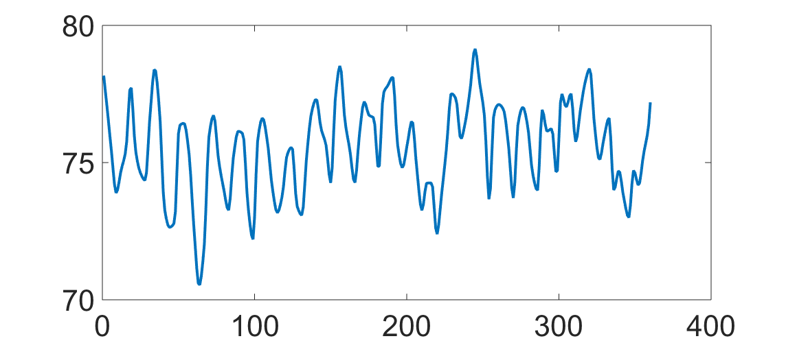
(a) Waking epoch

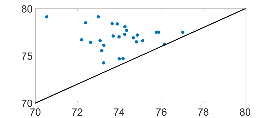
(b) $\mathcal{P}_{0}(H^{(k,j)})$

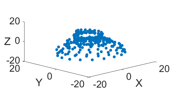
(c) $R_{120,1}(H^{k,j})$

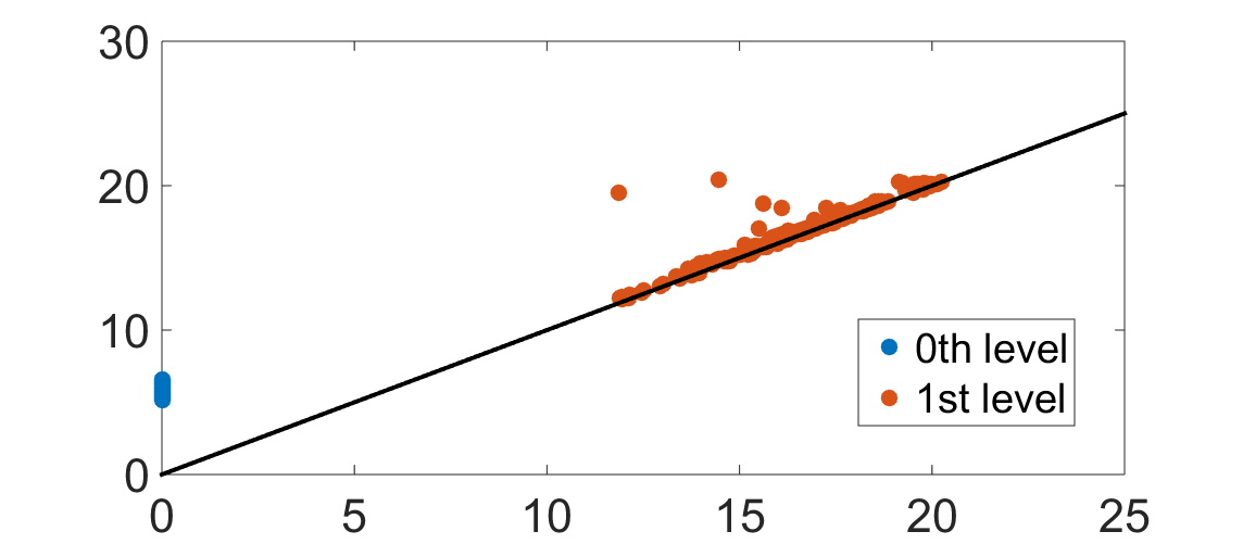
(d) $\mathcal{P}_{q}(R_{120,1}(H^{k,j}))$

Figure 5. An illustration of the IHR during the wake stage. (a) the IHR signal $H^{(k,j)}$; (b) the PD of the sub-level set filtration, $\mathcal{P}_{0}(H^{(k,j)})$; (c) The first three principal components of the point cloud $R_{120,1}(H^{k,j})$; (d) the PD’s of the VR filtration, $\mathcal{P}_{0}(R_{120,1}(H^{k,j}))$ and $\mathcal{P}_{1}(R_{120,1}(H^{k,j}))$ are superimposed, where blue and red points represent $q=0$ and $q=1$ respectively.

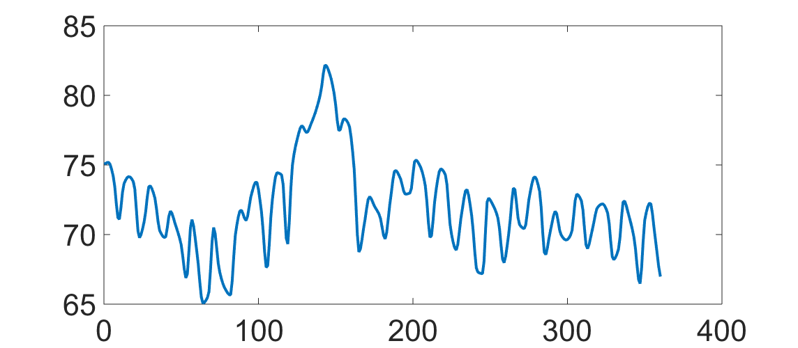
(a) Sleep epoch

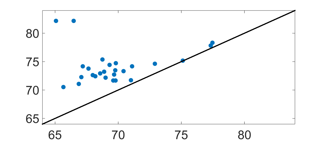
(b) $\mathcal{P}_{0}(H^{(k,j)})$

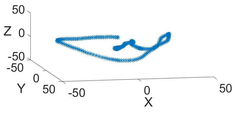
(c) $R_{120,1}(H^{k,j})$.

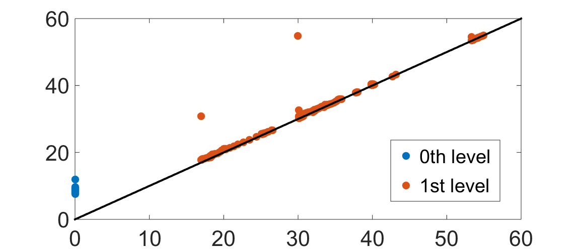
(d) $\mathcal{P}_{q}(R_{120,1}(H^{k,j}))$

Figure 6. An illustration of the IHR during the sleep stage. (a) the IHR signal $H^{(k,j)}$; (b) The PD of the sub-level set filtration, $\mathcal{P}_{0}(H^{(k,j)})$; (c) The first three principal components of the point cloud $R_{120,1}(H^{k,j})$; (d) the PD’s of the VR filtration $\mathcal{P}_{0}(R_{120,1}(H^{k,j}))$ and $\mathcal{P}_{1}(R_{120,1}(H^{k,j}))$ are superimposed, where blue and red points represent $q=0$ and $q=1$ respectively.

As discussed in Section 2.4, while it is possible to analyze the data via PD’s, it is usually computationally challenging. The proposed PS allows us to further summarize the PD’s and quantify the above observations. To examine the PS features, take $\cup_{k}\{\Phi^{(\texttt{PS})}(\mathcal{P}_{0}(H^{(k,j)}))\}_{j=1}^{n_{k}}$ as an example. In order to compare them on the same scale, we perform the standard $z$-score normalization for each subject. We abuse the notation and use $\Phi^{(\texttt{PS})}(\mathcal{P}_{0}(H^{(k,j)}))$ to denote the normalized parameters. In Fig. 7(a), we show the boxplot of each normalized PS parameter, where blue (red) bars represent the PS associated with an IHR time series associated with the sleep (wake) stage. We performed a rank sum test with the null hypothesis that two samples have equal medians with a significance level of $0.05$ with the Bonferroni correction. We found that there are significant differences between waking and sleeping features for all PS parameters, except for the kurtosis of $M$ (labeled as 4 in Fig. 7(a)), and the median of $L$ (labeled as 14 in Fig. 7(a)). The boxplot as shown in Fig. 7(a) shows that the mean and standard deviation of $M$ are the most distinguishable PS parameters between sleep and wake epochs. To further visualize these features, we apply the principle component analysis (PCA) to $\cup_{k}\{\Phi^{(\texttt{PS})}(\mathcal{P}_{0}(H^{(k,j)}))\}_{j=1}^{n_{k}}$, and plot the first three principal components in $\mathbb{R}^{3}$ as shown Fig. 7(b). We observe a separation between sleep and wake features. The visualization of $\Phi^{(\texttt{PS})}(\mathcal{P}_{i}(R_{120,1}(H^{k,j})))$, where $i=0,1$, is shown in Fig. SI.12.

Motivated by the above observation and discussion, we consider the following features for $H^{(k,j)}$ to distinguish sleep and wake epochs:

(17) $$[\Phi^{(\texttt{PS})}(\mathcal{P}_{0}(H^{(k,j)})),~{}\Phi^{(\texttt{PS})}(\mathcal{P}_{0}(R_{120,1}(H^{k,j}))),~{}\Phi^{(\texttt{PS})}(\mathcal{P}_{1}(R_{120,1}(H^{k,j})))].$$

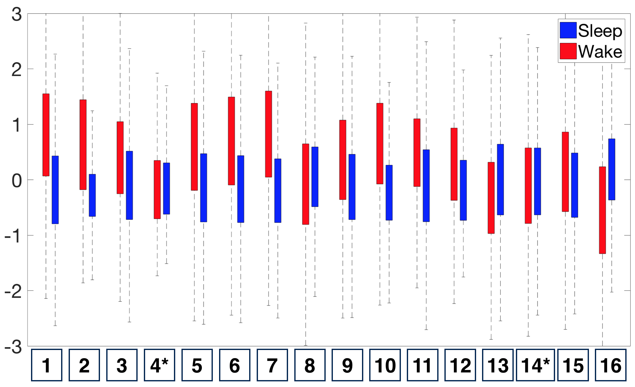
(a) Boxplot.

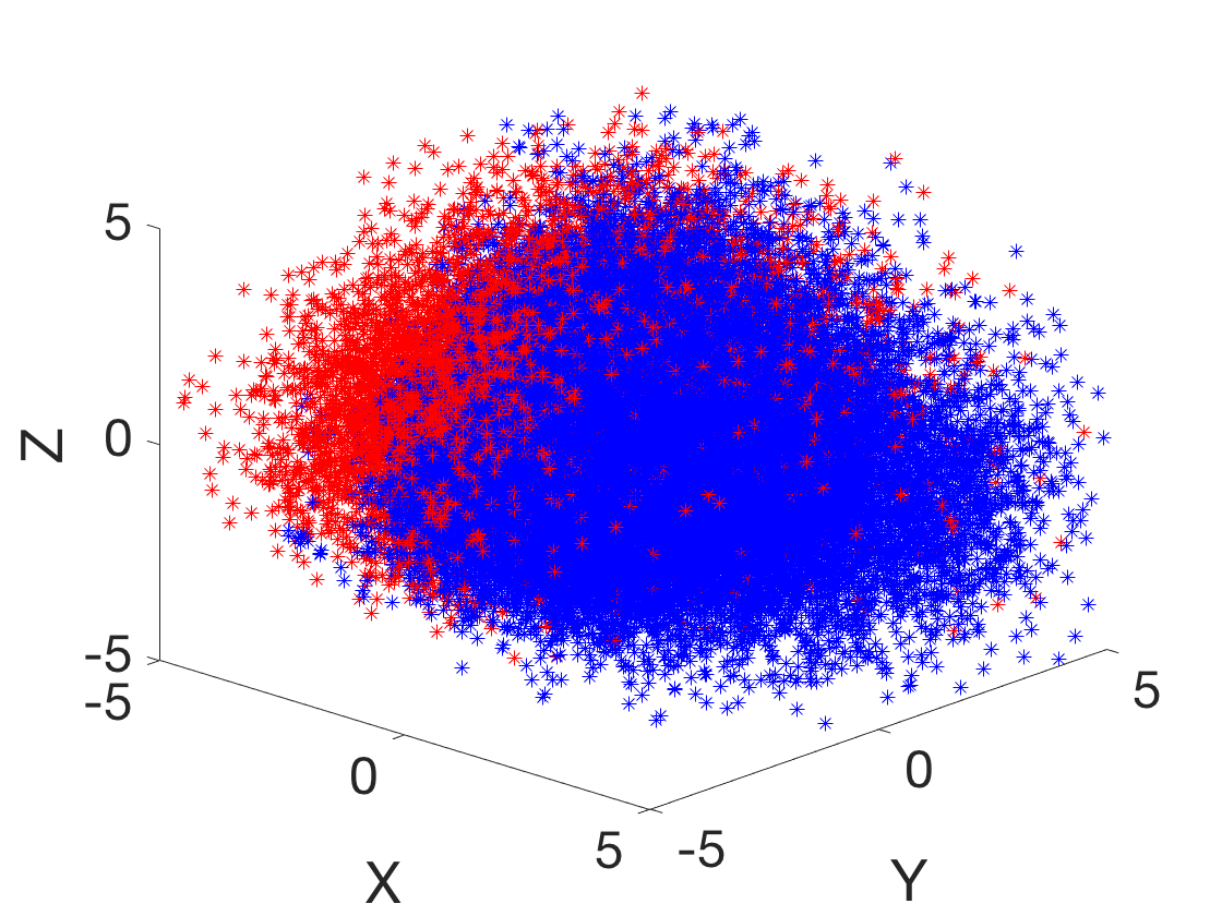
(b) Scatter plot.

Figure 7. Distribution of normalized PS features, $\Phi^{(\texttt{PS})}(\mathcal{P}_{0}(H^{(k,j)}))$. (a) Boxplot of the $\Phi^{(\texttt{PS})}(\mathcal{P}_{0}(H^{(k,j)})).$ The numbers listed on the horizontal axis indicates the number of PS. * indicates that the feature fails to reject the null hypothesis (that two samples have equal medians) of the significance level of $0.05$ on the rank sum test with Bonferroni correction. (b) Visualization of $\cup_{k}\{\Phi^{(\texttt{PS})}(\mathcal{P}_{0}(H^{(k,j)}))\}_{j=1}^{n_{k}}$ by the first three principal components.

4.4. Automatic sleep stage annotation system

4.4.1. Support Vector Machine as the learning model

We consider the widely applied classifier with a solid theoretical foundation, the support vector machine (SVM), to establish the heartbeat classification model. This is Step 4 (machine learning step) shown in Fig. 1. The linear function kernel is considered in this work and we use the Matlab built-in function fitcsvm with default parameters. The input data are features shown in (17), which are calculated by the publicly available libraries DIPHA (https://github.com/DIPHA/dipha) and Ripser (https://github.com/Ripser/ripser). When there are more than 2 classes, we apply the Error-Correcting Output Codes (ECOC) [28] with one-versus-one design. Specifically, we use the Matlab built-in function fitcecoc with default parameters. The Matlab version is 2014b.

4.4.2. Statistics

We carry out the cross-database validation. Specifically, we train the SVM model on one database, and evaluate the performance on the other databases. One of the main challenges in this automatic annotation problem is that the datasets are usually imbalanced; for example, the number of wake epochs is usually much smaller than that of sleep epochs (e.g., in the CGMH-training, the total number of wake epochs is $9,150$, while the total number of sleep epochs is $54,547$). In order to account for the imbalanced dataset, we adopt a down-sampling process. Let $E_{s}$ and $E_{w}$ be the collection of all sleep and wake epochs respectively across all subjects in the training set, and denote their cardinality by $|E_{s}|$ and $|E_{w}|$ respectively. We take all epochs in $E_{w}$, and randomly select $|E_{w}|$ epochs from $E_{s}$. The SVM model will then be built on these balanced epochs. Once the model is built on the training dataset, we test it on the entire testing dataset.

We report the following performance measurement indices. When there are $m$ labels, denote $M\in\mathbb{R}^{m\times m}$ to be the confusion matrix of the automatic classification model, where $M_{kl}$ represents the count of epochs whose known group labels are $k$ and whose predicted group labels are $l$. The sensitivity (SE), positive predictivity (+P) and F1 for the $k$-th class, the Cohen kappa, and the overall accuracy (Acc) are defined as

(18) $$SE_{k}=\frac{M_{kk}}{\sum_{l=1}^{m}M_{kl}},\,\,{+P_{k}=\frac{M_{kk}}{\sum_{l=1}^{m}M_{lk}}},\,\,{F1}_{k}=\frac{2(+P_{k})\cdot SE_{k}}{(+P_{k})+SE_{k}}$$

(19) $$Acc=\frac{\sum_{k=1}^{m}M_{kk}}{\sum_{k=1}^{m}\sum_{l=1}^{m}M_{kl}},\,\,Kappa=\frac{Acc-{EA}}{1-{EA}}$$

respectively, where EA means the expected accuracy and is defined by

(20) $${EA}=\frac{\sum_{p=1}^{m}\left(\sum_{q=1}^{m}M_{pq}\right)\times\left(\sum_{q=1}^{m}M_{qp}\right)}{\left(\sum_{p,q=1}^{m}M_{pq}\right)^{2}}.$$

When $m=3$, $k=1$ means wake, $k=2$ means REM, and $k=3$ means NREM. When classifying wake and sleep stages, $k=1$ means wake, and $k=2$ means sleep; when classifying REM and NREM stages, $k=1$ means REM, and $k=2$ means NREM. When $m=2$, $SE_{1}$ is reduced to the usual sensitivity (SE), $SE_{2}$ is reduced to the usual specificity (SP), and $+P_{1}$ is reduced to the precision (PR). For each database and each performance measurement, we report the mean $\pm$ standard deviation of all subjects.

All experiments in this and next sections were done using Windows 7 operating system environment equipped with i5-4570 CPU and 32 GB RAM. Under this computational environment, given a random seed, the whole training process of an SVM model takes $5\sim 7$ minutes on average. For the reproducibility purpose, the Matlab code is available in the GitHub repository website.

4.4.3. Automatic sleep stage classification result

We performed three classification tasks—sleep v.s. wake, REM v.s. NREM, and finally wake v.s. REM v.s. NREM. The random seed is fixed to $1$ in all cases when we ran the subsampling scheme. The results are shown in Tables 1, 2, and 3, where the SVM model was trained on the CGMH-training dataset and tested on CGMH-validation, DREAMS, and UCDSADB, respectively. For the interested readers, we also include extensive experimental results with different settings in SI.3, such as results of training on different datasets, and different random seeds. All results are similar to those reported in the main article.

Table 1. SVM cross-database performance of subjects for Wake and Sleep classification with a single random seed. The training database is CGMH-training. For each database and each performance measurement, we report the mean $\pm$ standard deviation of all subjects.

CGMH-training CGMH-validation DREAMS UCDSADB TP 76 $\pm$ 43 76 $\pm$ 44 101 $\pm$ 55 85 $\pm$ 44 FP 151 $\pm$ 49 126 $\pm$ 48 175 $\pm$ 61 149 $\pm$ 59 TN 462 $\pm$ 68 449 $\pm$ 102 592 $\pm$ 112 448 $\pm$ 110 FN 27 $\pm$ 33 42 $\pm$ 43 56 $\pm$ 45 73 $\pm$ 52 SE $(\%)$ 78.3 $\pm$ 14.7 70.9 $\pm$ 16.0 66.9 $\pm$ 16.1 57.6 $\pm$ 15.5 SP $(\%)$ 76.0 $\pm$ 6.1 78.9 $\pm$ 5.4 77.6 $\pm$ 5.8 75.3 $\pm$ 5.5 Acc $(\%)$ 75.2 $\pm$ 5.4 75.8 $\pm$ 4.4 74.7 $\pm$ 5.0 70.6 $\pm$ 5.4 PR $(\%)$ 34.0 $\pm$ 17.0 38.1 $\pm$ 19.6 37.0 $\pm$ 18.8 35.6 $\pm$ 17.3 F1 0.438 $\pm$ 0.161 0.452 $\pm$ 0.140 0.445 $\pm$ 0.146 0.407 $\pm$ 0.140 AUC 0.839 $\pm$ 0.084 0.824 $\pm$ 0.090 0.789 $\pm$ 0.090 0.702 $\pm$ 0.094 Kappa 0.320 $\pm$ 0.146 0.322 $\pm$ 0.123 0.308 $\pm$ 0.148 0.238 $\pm$ 0.133

Table 1 lists the result of classifying wake and sleep stages with different testing sets. For each testing database, we show the mean$\pm$standard deviation of each prediction outcome measurement of all subjects in that database. Table 1 shows the performances of training the model on CGMH-training and testing it on CGMH-validation, DREAMS, and UCDSADB. When considering the CGMH database, the (SE, SP) pair for CGMH-training and CGMH-validation are $(78.3\pm 14.7\%,76.0\pm 6.1\%)$ and $(70.9\pm 16.0\%,78.9\pm 5.4\%)$ respectively. When testing on DREAMS, the (SE, SP) pair becomes $(66.9\pm 16.1\%,77.6\pm 5.8\%)$. SP remains in the range of $70\%$, although SE falls below $70\%$. This result of the cross database testing is similar to that of validation result. When tested on UCDSADB, the pair of (SE, SP) becomes $(57.6\pm 15.5\%,75.3\pm 5.5\%)$. The overall performance on UCDSADB drops as expected since it contains sleep apnea subjects, and their sleep dynamics is disturbed by the sleep apnea. Overall, the cross-database validation results suggest that our model does not overfit. Moreover, we found that the down-sampling scheme alleviates the imbalance database issue.

Table 2 shows the performance for the REM and NREM classification. In this task, since the number of NREM epochs is much more than that of REM epochs, we apply the same down-sampling process to NREM as discussed in Section 4.4.2. Table 2 and Table 1 have several similarities.

Table 2. SVM cross-database performance for REM and NREM classification with a single random seed in the training procedure. The training database is CGMH-training. The subject $\#24$ in CGMH-validation and subject $\#9$ in UCDSADB were dropped because they do not have REM epochs. For each database and each performance measurement, we report the mean $\pm$ standard deviation of all subjects.

CGMH-training CGMH-validation DREAMS UCDSADB TP 75 $\pm$ 31 68 $\pm$ 30 93 $\pm$ 34 64 $\pm$ 34 FP 113 $\pm$ 32 106 $\pm$ 43 138 $\pm$ 51 133 $\pm$ 35 TN 400 $\pm$ 68 391 $\pm$ 94 490 $\pm$ 97 373 $\pm$ 68 FN 25 $\pm$ 23 20 $\pm$ 17 46 $\pm$ 27 50 $\pm$ 37 SE $(\%)$ 76.3 $\pm$ 16.0 78.1 $\pm$ 17.4 67.5 $\pm$ 16.7 58.0 $\pm$ 18.0 SP $(\%)$ 78.0 $\pm$ 4.8 79.6 $\pm$ 6.5 78.4 $\pm$ 5.2 73.7 $\pm$ 5.8 Acc $(\%)$ 77.4 $\pm$ 5.6 77.8 $\pm$ 8.3 76.3 $\pm$ 6.4 70.4 $\pm$ 6.4 PR $(\%)$ 39.4 $\pm$ 13.6 41.4 $\pm$ 19.0 41.0 $\pm$ 15.4 31.9 $\pm$ 16.0 F1 0.505 $\pm$ 0.138 0.510 $\pm$ 0.160 0.503 $\pm$ 0.144 0.390 $\pm$ 0.156 AUC 0.842 $\pm$ 0.094 0.849 $\pm$ 0.108 0.796 $\pm$ 0.115 0.711 $\pm$ 0.120 Kappa 0.382 $\pm$ 0.150 0.393 $\pm$ 0.175 0.312 $\pm$ 0.175 0.227 $\pm$ 0.162

Finally, Table 3 shows the performance for the wake, REM, and NREM classification. In this experiment, since the number of NREM is much more than those of wake and REM, the down-sampling scheme is applied to NREM. The Acc’s in all cases are about $60\%$, except the UCDSADB. The SE’s of wake, REM, and NREM are balanced and consistent across databases, except UCDSADB. Again, this result might be due to the fact that UCDSADB contains subjects with sleep apnea. On the other hand, note that the +P of NREM is higher than other classes, which is expected due to the dependence of +P on the database prevalence. In the Online Supplementary, we provide more cross-database validation results.

5. Discussion and Conclusion

In this work, the TDA tools are considered to analyze time series. Specifically, we propose a set of novel PS features to quantify HRV by analyzing IHR time series by TDA tools. The proposed HRV features are applied to predict sleep stages, ranging from wake, REM and NREM. In addition to being computationally efficient, the algorithm is theoretically sound supported by mathematical and statistical results. Note that while we focus on the HRV analysis for the sleep stage annotation, the proposed algorithm has a potential to be applied to analyze other time series and study the HRV for other clinical problems.

Table 3. SVM cross-database performance for Wake, REM and NREM classification with a single random seed in the training procedure. The training database is CGMH-training. The subject $\#24$ in CGMH-validation and the subject $\#9$ in UCDSADB were dropped because they do not have REM epochs. For each database and each performance measurement, we report the mean $\pm$ standard deviation of all subjects.

CGMH-training CGMH-validation DREAMS UCDSADB SE $(\%)$ (Wake) 63.7 $\pm$ 15.3 61.1 $\pm$ 19.0 56.2 $\pm$ 14.5 39.5 $\pm$ 11.9 SE $(\%)$ (REM) 62.8 $\pm$ 17.4 67.1 $\pm$ 20.9 57.0 $\pm$ 18.0 48.4 $\pm$ 19.6 SE $(\%)$ (NREM) 71.9 $\pm$ 6.7 72.6 $\pm$ 6.4 72.5 $\pm$ 6.8 66.0 $\pm$ 7.6 +P $(\%)$ (Wake) 40.6 $\pm$ 19.1 43.7 $\pm$ 16.6 44.1 $\pm$ 18.3 39.3 $\pm$ 17.9 +P $(\%)$ (REM) 39.1 $\pm$ 14.9 40.0 $\pm$ 17.7 39.4 $\pm$ 15.5 28.5 $\pm$ 15.8 +P $(\%)$ (NREM) 89.3 $\pm$ 8.8 85.6 $\pm$ 16.0 83.7 $\pm$ 8.6 76.6 $\pm$ 9.2 Acc $(\%)$ 68.3 $\pm$ 6.4 67.6 $\pm$ 9.2 66.3 $\pm$ 6.4 57.1 $\pm$ 7.1 Kappa 0.401 $\pm$ 10.2 0.390 $\pm$ 0.117 0.372 $\pm$ 0.116 0.244 $\pm$ 0.108

5.1. Theoretical Supports and Open Problems

We find that empirically, $M$ and $L$ are simple yet effective representations of the PD and reveal signatures about the underlying object. It would be interesting to investigate, in theory, the probability distribution of $M$ and $L$ for a given simplicial complex. However, to the best of our knowledge, while there have been several works in this direction, it is still a relatively open problem. Recently, there has been some theoretical work towards this direction, namely the theory of random complexes (see e.g. survey papers [13, 42] and references therein). In order to understand the role of noises in the PD, there have been studies on the topology of the noise. In the theory of random fields, authors in [54] used sub-level sets as filtration to study the number of components ($\beta_{0}$) with various random processes; in [2], authors studied the relation between random fields and the PH in general. In particular, as mentioned in [2]: “It would be interesting to know more about the real distributions lying behind the PD, but at this point we know very little.” There is also a result in random cubical complexes [40], and a few work on the limiting theorem of total sum persistence [58] and persistence diagrams [40]. It would also be interesting to study the stability of each PS. As of now, only the sum of $L$, the max of $L$, and the entropy of $L$ have been shown to be stable [25, 6]. However, the rest of PS is still unknown. Another interesting direction, instead of focusing on each PS, is to study the probability distributions of $M$ and $L$. For instance, let $\rho_{M}$ and $\rho_{L}$ be the empirical probability density function of the sets $M$ and $L$, respectively. For $S=M$ or $S=L$, could one establish $\|\rho_{S}(f)-\rho_{S}(g)\|_{D}\leq d_{B}(\mathcal{P}_{q}(f),\mathcal{P}_{q}(g))$, where $\|\cdot\|_{D}$ is some suitable statistical distance? We leave those interesting theoretical problems to future work.

5.2. Comparison with existing automatic sleep stage annotation results

There have been several results in automatic sleep stage annotation by taking solely the HRV into account. A common conclusion is that classifying sleep-wake by quantifying HRV is a challenging job. In general, due to the heterogeneity of the data sets, various evaluation criteria and different features and models used in these publications, it is difficult to have a direct comparison. But to be fair, below we summarize some related existing literatures for a discussion. To the best of our knowledge, except [50], there is no result reporting a cross-database validation. For those running validation on a single database, we shall distinguish two common cross validation (CV) schemes – leave-one-subject-out CV (LOSOCV) and non-LOSOCV. When the validation set and the training set come from different subjects, we call it the LOSOCV scheme; otherwise we call it the non-LOSOCV scheme. The LOSOCV scheme is in general challenging due to the uncontrollable inter-individual variability, while the non-LOSOCV scheme tends to over-estimate. Therefore, for a fair comparison, below we only summarize papers considering only the IHR features and carrying out the LOSOCV scheme.

In [82], the database was composed of healthy participants aged $16-61$ years. A random forest model was established to differentiate between the wake, REM, and NREM stages for those epochs labeled as “stationary”. Based on the confusion matrix provided in [82], the SE, SP, Acc, and F1 for detecting the wake stage are $51.2$%, $90.2$%, $84.0$%, and $0.50$. The authors also provided the SE of wake, REM, and NREM, which are $53.72\%\pm 20.15\%$, $59.01\%\pm 19.72\%$, and $79.50\%\pm 7.82\%$ respectively. In Table 3, our validation on CGMH-validation is $61.1\pm 19.0\%$, $67.1\pm 20.9\%$, and $72.6\pm 6.4\%$, respectively. Observe that our SE of wake and REM are better, and SE of NREM is on the similar level. In addition to the balance of all classes due to the sub-sampling scheme in our result, note that we focus on all epochs but not “stationary epochs”, and the subjects in CGMH-validation are not healthy but simply without sleep apnea.

In [52], the database was composed of 24 participants aged $40-50$ years with $0$ AHI. The authors took the temporal information and the phase and magnitude of the “sleepy pole” as features to train a hidden Markov model to differentiate REM and NREM stages. The reported SE, SP, and Acc were $70.2\%$, $85.1\%$, and $79.3\%$, respectively. Our results outperform theirs. Our SE, SP and Acc of the REM and NREM classification in CGMH-validation shown in Table 2 are $78.1\pm 17.4\%$, $79.6\pm 6.5\%$, and $77.8\pm 8.3\%$, respectively. Observe that both Accs are similar which means portion of correct predictions are similar. Not only our SE is better, but SE and SP are also balanced.

In [48], the database is composed of 190 infants. A variety of features and classification algorithms were considered and the wake and sleep classes were balanced for the analysis. The SE and SP of their multi-layer perceptron model without rejection was $79.0\%$ and $77.5\%$, respectively. In Table 1, the SE and SP of our result on CGMH-validation is $70.9\pm 16.0\%$ and $78.9\pm 5.4\%$. Our performance is comparable to theirs. However, there is a fundamental difference between their experiments and ours – the sleep dynamics of infants and adults are different.

In [3], the database is composed of $20$ participants aged $49$-$68$ years with varying degrees of sleep apnea. Detrended fluctuation analysis and a feed-forward neural network were applied to differentiate the wake and sleep stages. Various epoch lengths were considered, and the highest performance was recorded on an epoch length of $5$ minutes. The Acc, SE, SP, and Cohen’s kappa were $71.9\pm 18.2\%$, $43.7\pm 27.3\%$, $89.0\pm 7.8\%$, and $0.29\pm 0.24$, respectively. We consider UCDSADB for a comparison. In Table 1, the Acc, SE, SP, and Cohen’s kappa of our testing result on UCDSADB is $70.6\pm 5.4\%$, $57.6\pm 15.5\%$, $75.3\pm 5.5\%$, and $0.238\pm 0.133$. Their Acc and ours are on the same level, our SE is better than theirs, while their SP is better than ours. However, our SE and SP are balanced compared with theirs. A major difference is that our standard deviations for Acc, SE, SP are much smaller. Thus, our performance is comparable to theirs.

In [49], fifteen participants aged $31.0\pm 10.4$ years with the Pittsburgh Sleep Quality Index less than $6$ were considered. The linear discriminant-based classifier was trained with spectral HRV features. The SE, SP, Cohen’s kappa and AUC were $49.7\pm 19.2\%$, $96\pm 3.3\%$, $0.48\pm 0.24$ and $0.54$ respectively. As shown in Table 1, the SE, SP, Cohen’s kappa and AUC of our result on CGMH-validation is $70.9\pm 16.0\%$, $78.9\pm 5.4\%$, $0.322\pm 0.123\%$, and $0.824\pm 0.090$, respectively. Again, compared with their results, our SE and SE are more balanced.

To make a conclusion, we emphasize that all those results under comparison are not carried out in the cross-database scheme. Also, usually the SE and SP are not balanced with high SP, which leads to the high accuracy. Therefore, the results suggest that the proposed PS features and chosen learning model lead a better, or at least similar, performance compared with the state-of-the-art results. The cross-database validation further suggests the usability of the PS features and the proposed learning scheme in clinical setups. Last but not the least, due to the numerical efficiency of the proposed PS features, it is potential to apply it to analyze large scale time series.

5.3. Technical issues

We remark that although it is possible to include $\mathcal{P}_{i}(R_{120,1}(H^{k,j}))$ for $i\geq 2$ in (17), in practice, it is a challenging task due to its computational complexity. Its computation is known to be poorly scalable in dimension and memory-intensive. We refer readers to [57] for more details and comparisons among state-of-arts TDA packages and extensive benchmark. To get an idea of the computational cost, for any epoch, the computational time by the state-of-art package Ripser for $\mathcal{P}_{1}(R_{120,1}(H^{k,j}))$, $\mathcal{P}_{2}(R_{120,1}(H^{k,j}))$, and $\mathcal{P}_{3}(R_{120,1}(H^{k,j}))$ are $0.06$, $1.7$, and $106$ seconds in a standard laptop, respectively. This echos the fact that the computation of $\mathcal{P}_{i}(R_{120,1}(H^{k,j}))$ does not scale well in $i$ [57]. Thus, it would be inefficient to obtain the higher dimensional persistence features.

5.4. Limitations and future directions

In addition to the theoretical development discussed above, there are several interesting practical problems left untouched. While we systematically consider the inter-individual variance, the race, the machine, and the sleep disorder by taking three different databases into account, we acknowledge the fact that the data is collected from the sleep lab. When the data is collected from the real-world mobile device, it is not clear if the algorithm could perform as well and run in real-time. Moreover, its performance for the home-based screening needs to be further evaluated. Yet, in the current mobile health market, the photoplethysmography (PPG) sensor has been widely applied, and its applicability for the sleep-wake classification has been reported in [50]. It is interesting to see how the TDA approach could be applied to analyze the HRV from the PPG for the sleep stage classification mission. From the data analysis perspective, it would be interesting to perform a more sophisticated analysis and take other features from the PD. For instance, the PH Transformation (PHT) [75] was recently developed and proven to be a sufficient statistic, and had been successfully applied to the shape analysis. It would be interesting to combine the PHT and PS. IHR is a well-known non-stationary time series. Based on the encouraging results of applying the TDA, we suspect that the PS features could be applied to study other clinical problems related to HRV, and furthermore, analyze other physiological time series. We will explore those limitations/directions in our future work.

Appendix SI.1 More Mathematical Background

SI.1.1. More Simplicial Complexes

To investigate the complicated structure of an object, an intuitive way is to use simple objects as building blocks to approximate the original object. For instance, in computer graphics, curves and surfaces in Euclidean spaces are approximated by line segments and triangles, e.g. Figure SI.9 (D). In TDA, the main building blocks are simplicial complexes. Simplicial complexes are important tools to approximate continuous objects via combinatorial objects, such as vertices, edges, faces, and so on. Although simplicial complexes and simplicial homology can be studied in an abstract and general way (see e.g. [30, 56]), to enhance the readability, we present the notion in a relatively concrete way without losing critical information.

We start with introducing simplex. Intuitively, a simplex is a “triangle” in different dimension. As shown in Figure SI.8, vertices, line segments, triangles and tetrahedron in $\mathbb{R}^{d}$ are $0,1,2,3$-dimensional triangles respectively, and they are called $0$-simplexes, $1$-simplexes, $2$-simplexes and $3$-simplexes in $\mathbb{R}^{d}$ respectively. The formal definitions can be found below.

Definition 7 ([56] Sec. 1.1, p. 3).

Let $x_{0},x_{1},\ldots,x_{q}$ be affinely independent points in $\mathbb{R}^{d}$. The $q$-simplex, denoted by $\sigma:=\langle x_{0},x_{1},\ldots,x_{q}\rangle$, is defined to be the convex hull of $x_{0},x_{1},\ldots,x_{q}$. In other words,

$$\sigma=\left\{\lambda_{0}x_{0}+\lambda_{1}x_{1}+\cdots+\lambda_{q}x_{q}\ \left|\ \lambda_{0},\lambda_{1},\ldots,\lambda_{q}\in[0,1],\sum_{i=0}^{q}\lambda_{i}=1\right.\right\}.$$

We denote ${\rm Vert}(\sigma):=\{x_{0},x_{1},\ldots,x_{q}\}$.

Recall that $x_{0},x_{1},\ldots,x_{q}$ are affinely independent points in $\mathbb{R}^{d}$ if and only if $x_{1}-x_{0},\ldots,x_{q}-x_{0}$ are linearly independent vectors in $\mathbb{R}^{d}$. Any $q$-simplex is a $q$ dimensional object, and it consists of lower degree simplexes. We are interested in the relation among simplexes of different dimensions. Since any subset $V$ of ${\rm Vert}(\sigma)$ is also affinely independent, the convex hull of $V$ also forms a simplex with dimensional $|V|\leq q$ where $|V|$ denotes the cardinality of $V$. This lower dimensional simplex is called a face of $\sigma$.

Definition 8 ( [56] Sec. 1.1, p. 5).

Let $\sigma$ be a $q$-simplex, and $V\subset{\rm Vert}(\sigma)$. The convex hull of $V$ is called a face of $\sigma$. Moreover, if $|V|=k$, then the face $\tau=\langle V\rangle$ is called a $k$-face of $\sigma$.

For example, in Figure SI.8, the $3$-simplex (tetrahedron) $\langle G,H,I,J\rangle$ has the following faces:

• $0$-face: $\langle G\rangle$, $\langle H\rangle$, $\langle I\rangle$ and $\langle J\rangle$;

• $1$-face: $\langle G,H\rangle$, $\langle G,I\rangle$, $\langle G,J\rangle$, $\langle H,I\rangle$, $\langle H,J\rangle$ and $\langle I,J\rangle$;

• $2$-face: $\langle G,H,I\rangle$, $\langle G,I,J\rangle$, $\langle G,H,J\rangle$ and $\langle H,I,J\rangle$.

A simplicial complex $\mathcal{K}$ in $\mathbb{R}^{d}$ is a collection of finite simplexes $\sigma$ in $\mathbb{R}^{d}$ so that any intersection of two arbitrary simplexes is a face to each of them. It is formalized in the following definition.

Definition 9 ([56] Sec. 1.2, p. 7).

A collection $\mathcal{K}$ of simplexes in $\mathbb{R}^{d}$ is said to be a simplicial complex if it satisfies the following two properties:

• If $\sigma\in\mathcal{K}$ and $\tau$ is a face of $\sigma$, then $\tau\in\mathcal{K}$;

• If $\sigma_{1},\sigma_{2}\in\mathcal{K}$, then $\sigma_{1}\cap\sigma_{2}$ is a face of $\sigma_{1}$ and $\sigma_{2}$. In particular, $\sigma_{1}\cap\sigma_{2}\in\mathcal{K}$.

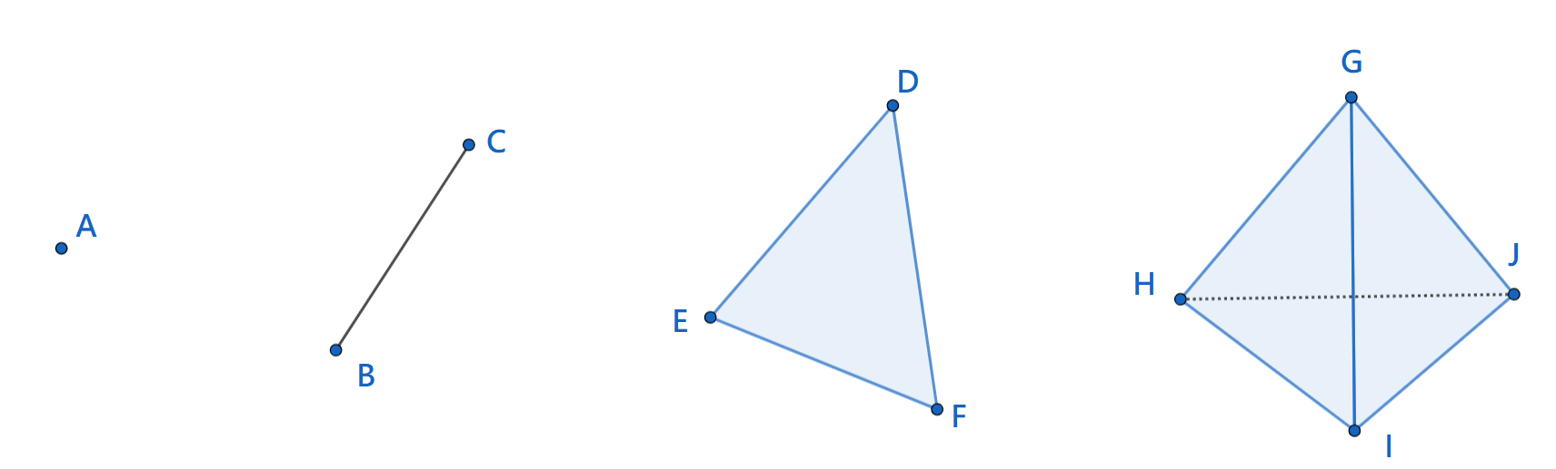
Figure SI.8. Illustration of simplices in dimension $0,1,2,3$. The singleton point $\{A\}$ forms a $0$-simplex and convex hulls $\langle B,C\rangle$, $\langle D,E,F\rangle$ and $\langle G,H,I,J\rangle$ are $1$-simplex, $2$-simplex, $3$-simplex in an Euclidean space respectively.

For instance, the surface in Figure SI.9(D) is represented by a simplicial complex consisting of simplexes with maximal dimension 2, that is, triangles and their edges and vertices.

In order to study the topological information of a given simplicial complex, we study relations among different dimensional simplexes. It can be understood as a way to measure the complexity of simplicial complexes. Homology theory is the main theory we count on to achieve this goal. In the end, we will define the Betti numbers.

SI.1.2. More on Betti numbers and Homology

Homology is a classic subject in algebraic topology [56], which captures “holes” of geometric objects in different dimensions. While we can discuss homology in more general geometric objects, in this work, we mainly consider simplicial complexes as our target object. We now discuss how to quantify $q$-dimensional holes.

In order to count $q$-dimensional holes in $\mathcal{K}$, we need to find the interactions among different simplexes. To achieve it, one adds an algebraic structure to simplexes. Formally, given $q$-simplex $\sigma_{1},\sigma_{2},\ldots,\sigma_{n}\in\mathcal{K}$, one could write a formal sum as $c=\sum_{i=1}^{n}\nu_{i}\sigma_{i}$, where $\nu_{i}\in\mathbb{Z}_{2}$. This formal sum is commonly known as a $q$-chain. One could also define an addition as $\sum_{i=1}^{n}\nu_{i}\sigma_{i}+\sum_{i=1}^{n}\mu_{i}\sigma_{i}:=\sum_{i=1}^{n}(\nu_{i}+\mu_{i})\sigma_{i}$. We consider the collection of all $q$-chains, denoted by

(SI.1) $$C_{q}(\mathcal{K}):=\bigg{\{}\sum_{i=1}^{n}\nu_{i}\sigma_{i}~{}\Big{|}~{}\nu_{i}\in\mathbb{Z}_{2},~{}\sigma_{i}\in\mathcal{K},~{}\dim(\sigma)=q\bigg{\}}.$$

One could prove that $C_{q}(\mathcal{K})$ is actually a vector space over $\mathbb{Z}_{2}$ with the above addition. For example, consider the simplicial complex $\mathcal{K}=\langle D,E,F\rangle$ in Figure SI.8. $\langle D\rangle+\langle E\rangle$ is an element in $C_{0}(\mathcal{K})$, and $\langle D,E\rangle+\langle E,F\rangle$ is an element in $C_{1}(\mathcal{K})$. Note that $\langle D,E\rangle+\langle E\rangle$ is not defined because they live in different spaces. There is a natural relation between $C_{q}(\mathcal{K})$ and $C_{q-1}(\mathcal{K})$, called the boundary map.

Definition 10 ([56] Sec. 1.5, p. 30).

Let $\sigma=\langle x_{0},x_{1},\cdots,x_{q}\rangle\in C_{q}(\mathcal{K})$. The $q^{\rm th}$ boundary map $\partial_{q}:C_{q}(\mathcal{K})\rightarrow C_{q-1}(\mathcal{K})$ over $\mathbb{Z}_{2}$ is defined by

(SI.2) $$\partial_{q}(\langle x_{0},x_{1},\cdots,x_{q}\rangle)=\sum_{i=0}^{q}\langle x_{0},\cdots,\widehat{x_{i}},\cdots x_{q}\rangle,$$

where $\sigma=\langle x_{0},x_{1},\cdots,x_{q}\rangle$ being a $q$-simplex in $\mathcal{K}$ and the $\widehat{\bullet}$ denotes the drop-out operation.

For instance, $\partial_{2}(\langle D,E,F\rangle)=\langle E,F\rangle+\langle D,F\rangle+\langle D,E\rangle$. $\partial_{q}$ captures the boundary of a given simplex, which justifies the nomination. With the boundary maps, there is a nested relation among chains

(SI.3) $$\cdots\xrightarrow[]{\partial_{n+1}}C_{n}(\mathcal{K})\xrightarrow[]{\partial_{n}}C_{n-1}(\mathcal{K})\xrightarrow[]{\partial_{n-1}}\cdots C_{1}(\mathcal{K})\xrightarrow[]{\partial_{1}}C_{0}(\mathcal{K}).$$

This nested relation among chains is known as the chain complex, which is denoted as $\mathcal{C}=\{C_{q},\partial_{q}\}_{q\in\mathbb{Z}}$.

A fundamental result in homology theory ([56] Lemma 5.3 Sec. 1.5, p. 30) is that the composition of any two consecutive boundary maps is a trivial map, i.e. $\partial_{q-1}\circ\partial_{q}=0$. This result allows one to define the following quotient space. We first denote cycles and boundaries by $Z_{q}$ and $B_{q}$, respectively, which are defined as

(SI.4) $$Z_{q} :=\ker(\partial_{q})=\{c\in C_{q}\ |\ \partial_{q}(c)=0\},$$

$$B_{q} :={\rm im}(\partial_{q+1})=\{\partial_{q+1}(z)\in C_{q}\ |\ z\in C_{q+1}\}.$$

Note that each $B_{q}$ is a subspace of $Z_{q}$. Therefore, we can define the $q^{\rm th}$ homology to be the quotient space

(SI.5) $$H_{q}(\mathcal{K}):=\frac{Z_{q}}{B_{q}}=\frac{\ker(\partial_{q})}{{\rm im}(\partial_{q+1})},$$

which is again a vector space. Finally, the Betti number is defined to be the dimension of the homology. More precisely,

(SI.6) $$\beta_{q}(\mathcal{K})=\dim(H_{q}(\mathcal{K})).$$

As a result, given a simplicial complex $\mathcal{K}$, the homology of $\mathcal{K}$ is a collection of vector spaces $\{H_{q}(\mathcal{K})\}_{q=0}^{\infty}$, and its Betti numbers is denoted as $\beta(\mathcal{K}):=\{\beta_{q}(\mathcal{K})\}_{q=0}^{\infty}$. Formally speaking, $\beta_{q}$ measures the number of $q$-dimensional holes. For instance, $\beta_{0}$ counts the number of components, $\beta_{1}$ counts the number of loops, and $\beta_{2}$ counts the number of voids. Using this intuition and by visual inspection, one may count the Betti numbers of those simplicial complexes appeared in Figure SI.9.

Figure SI.9 shows some examples of simplicial complexes in $\mathbb{R}^{2}$, $X_{1}$ to $X_{3}$, and $\mathbb{R}^{3}$, $X_{4}$ to $X_{6}$. For instance, the direct computation shows that $H_{0}(X_{1})=\mathbb{Z}_{2}$, $H_{1}(X_{1})=\mathbb{Z}_{2}$, and $H_{q}(X_{1})=\{0\}$ for all $q>1$; hence $\beta(X_{1})=\{1,1,0,\ldots\}$. The only nontrivial homology group of $X_{2}$ is $H_{0}(X_{2})=\mathbb{Z}_{2}^{2}$, and hence $\beta(X_{2})=\{2,0,\ldots\}$. For objects $X_{4}$ to $X_{6}$, voids in $\mathbb{R}^{3}$ surrounded by spheres or tori are $2$-dimensional holes, so $H_{2}(X_{5})=\mathbb{Z}_{2}^{5}$ and $H_{2}(X_{6})=\mathbb{Z}_{2}$. Note that $H_{1}(X_{6})=\mathbb{Z}_{2}^{2}$ because a torus has two $1$-dimensional holes ([56] Theorem 6.2 Sec. 1.6, p. 35).

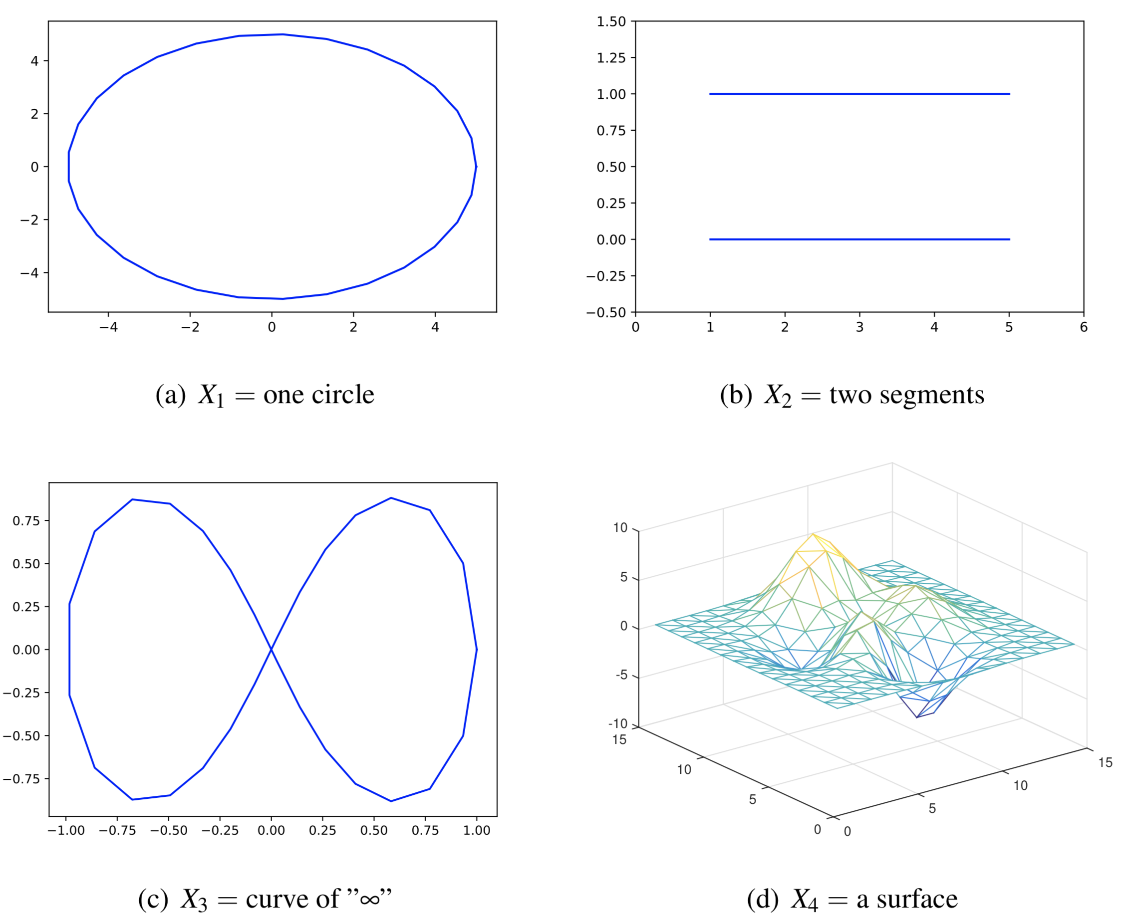
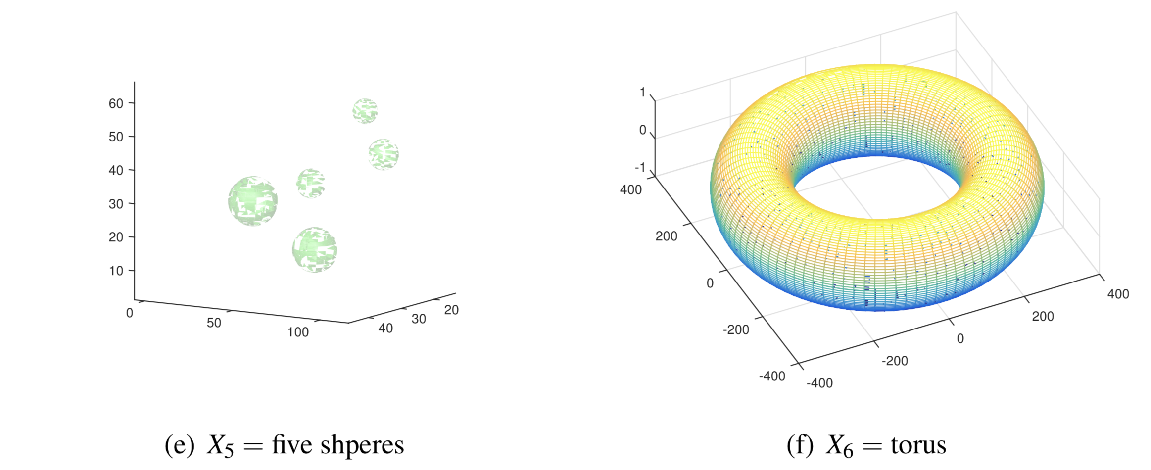
Figure SI.9. Some examples of geometric objects in $\mathbb{R}^{2}$ and $\mathbb{R}^{3}$. The Betti numbers are: $\beta(X_{1})=(1,1)$, $\beta(X_{2})=(2,0)$, $\beta(X_{3})=(1,2)$, $\beta(X_{4})=(1,0,0)$, $\beta(X_{5})=(5,0,5)$ and $\beta(X_{6})=(1,2,1)$.

SI.1.3. More about sub-level set and VR filtrations

First, we provide an example of the sublevel set filtration.

Example SI.1.3.1.

Consider a simple filtration $\{f_{1.5},f_{2.5},f_{3}\}$ as shown in Figure SI.10. When $h=1.5$, the sub-level set $f_{1.5}$ has $\beta_{0}=2$ since it contains two connected components i.e., disjoint intervals in $\mathbb{R}^{1}$. When $h=2.5$, two connected components in $f_{1.5}$ merged to $f_{2.5}$. Moreover, there is a new interval ($\approx[0.8,0.9]$) appeared in $f_{2.5}$, and hence $\beta_{0}(f_{2.5})=2$. Finally, when $h$ is lifted to $3$, previous intervals are merged to $f_{3}$ and we get $\beta_{0}(f_{3})=1$. This filtering process can be depicted in the PD as shown in Figure SI.10(D), which is $\mathcal{P}_{0}(\{f_{1.5},f_{2.5},f_{3}\})=\{(1.5,\infty),(1.5,2.5),(2.5,3)\}$.

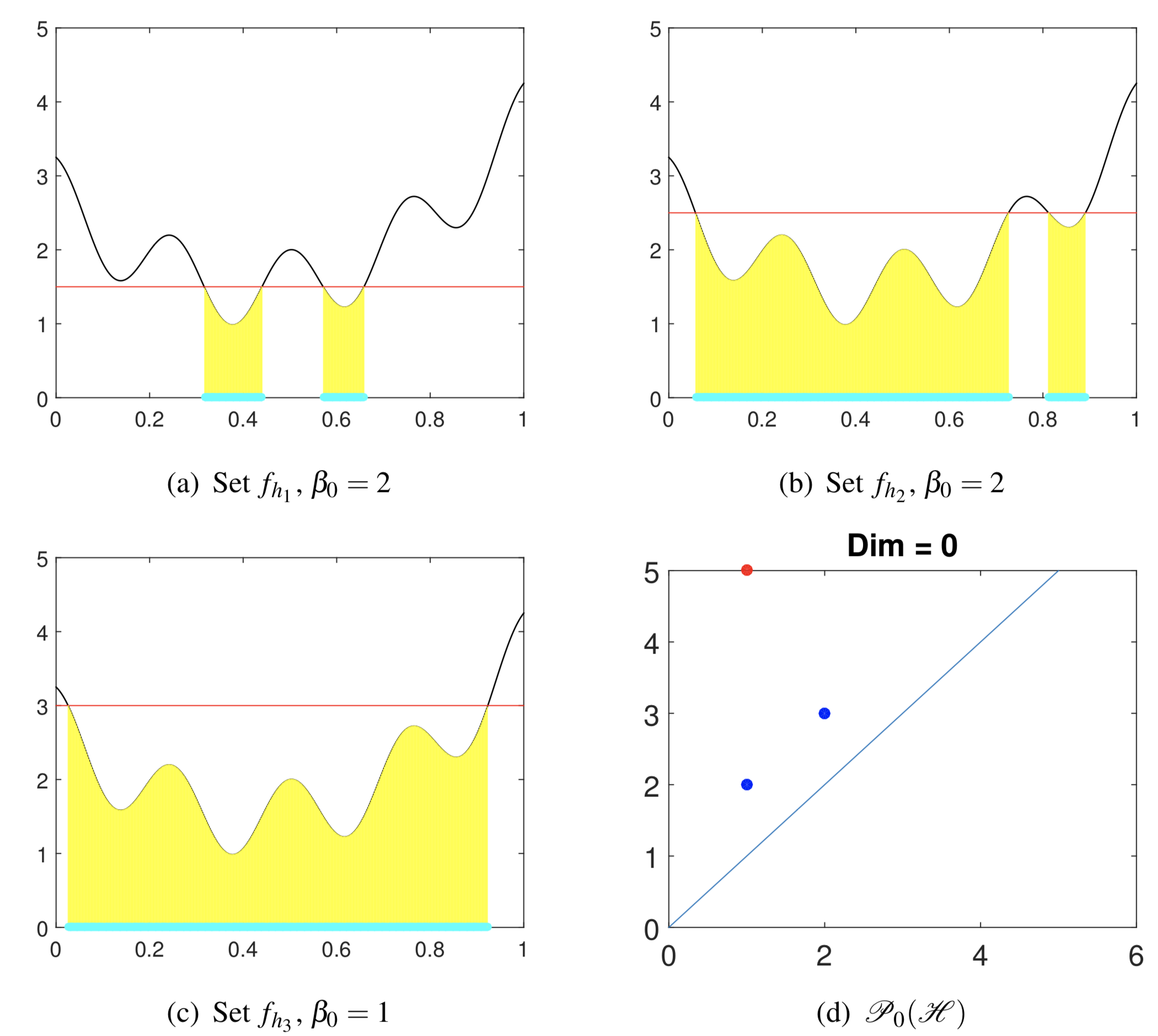
Figure SI.10. An example of sub-level sets of signal $f(t)=1+t+7(t-0.5)^{2}+\cos(8\pi t)/2$. Unions of blue line segments lying on $x$-axis in terms $(a)$, $(b)$ and $(c)$ are sub-level sets $f_{h_{1}},f_{h_{2}}$ and $f_{h_{3}}$ ($h_{1}=1.5$, $h_{2}=2.5$, $h_{3}=3$) with corresponding thresholds. We also use the convention $f_{h_{1}}=I_{1,{\rm left}}\cup I_{1,{\rm right}}$ and $f_{h_{2}}=I_{2,{\rm left}}\cup I_{2,{\rm right}}$ to decompose $f_{h_{1}}$ and $f_{h_{2}}$ by disjoint intervals as blue line segments in $(a)$ and $(b)$. Labels of $x,y$ axes in $(a)$, $(b)$ and $(c)$ are arbitrary units.

Next, we show an illustrative example of the VR filtration.

Example SI.1.3.2.

Figure SI.11 shows an example of VR complex of point-cloud in $\mathbb{R}^{2}$, where points are sampled from curve $X_{3}$ in Figure SI.9. As in Figure SI.11, when $\epsilon$ is too small, then the information of Betti numbers of the simplicial complex ${\rm VR}(X;\epsilon)$ is nothing different to original point-cloud. On the other hand, for extremely large $\epsilon$, the only non-zero Betti number of ${\rm VR}(X;\epsilon)$ is $\beta_{0}=1$. For example, the only two $1$-dimension holes in filtration $\mathcal{K}_{1}\subseteq\mathcal{K}_{2}\subseteq\cdots\subseteq\mathcal{K}_{6}$ of Figure SI.11 were born at time $5$ ($\mathcal{K}_{5}$) and died at time $6$ ($\mathcal{K}_{6}$), hence both of them have coordinate $(5,6)$. Moreover, if a $q$-dimensional hole is still alive in the final object of the filtration, we will use $\infty$ to denote its death value (which indicates the feature never dies). We also use Figure SI.11 to explain the PD. First, in every $\mathcal{K}_{i}$, we encode each component to the smallest index of points belonging to the components. For example, because vertices $5$ and $14$ represent the same connected component $\langle 5,14\rangle$ in $\mathcal{K}_{1}$, we use $0$-simplex $\langle 5\rangle$ to denote the component.

With the VR complex, the lifespan of each hole can be computed. For example, both of components $\langle 5\rangle$ and $\langle 11\rangle$ in $\mathcal{K}_{1}$ has life span $(1,2)$ because they would be merged into the connected component represented by $\langle 4\rangle$ in $\mathcal{K}_{2}$. On the other hand, because the connected component $\langle 0\rangle$ is alive in whole filtration, it has lifespan $(1,\infty)$. As a result, the PD of filtration in Figure SI.11 can be expressed as

(SI.7) $$\begin{split}\mathcal{P}_{0}(\mathcal{K})=&\{(1,\infty)_{\langle 0\rangle},(1,4)_{\langle 1\rangle},(1,2)_{\langle 2\rangle},(1,2)_{\langle 3\rangle},(1,3)_{\langle 4\rangle},(1,2)_{\langle 5\rangle},\\ &\ \ (1,2)_{\langle 6\rangle},(1,2)_{\langle 7\rangle},(1,2)_{\langle 8\rangle},(1,3)_{\langle 9\rangle},(1,3)_{\langle 10\rangle},(1,2)_{\langle 11\rangle},\\ &\ \ (1,2)_{\langle 12\rangle},(1,2)_{\langle 13\rangle},(1,2)_{\langle 15\rangle},(1,3)_{\langle 16\rangle},(1,2)_{\langle 17\rangle},(1,2)_{\langle 18\rangle}\}\end{split}$$

and $\mathcal{P}_{1}(\mathcal{K})=\{(5,6),(5,6)\}$. The notations $\langle*\rangle$ of lifespans in (SI.7) are used for clarifying which component a lifespan belong to.

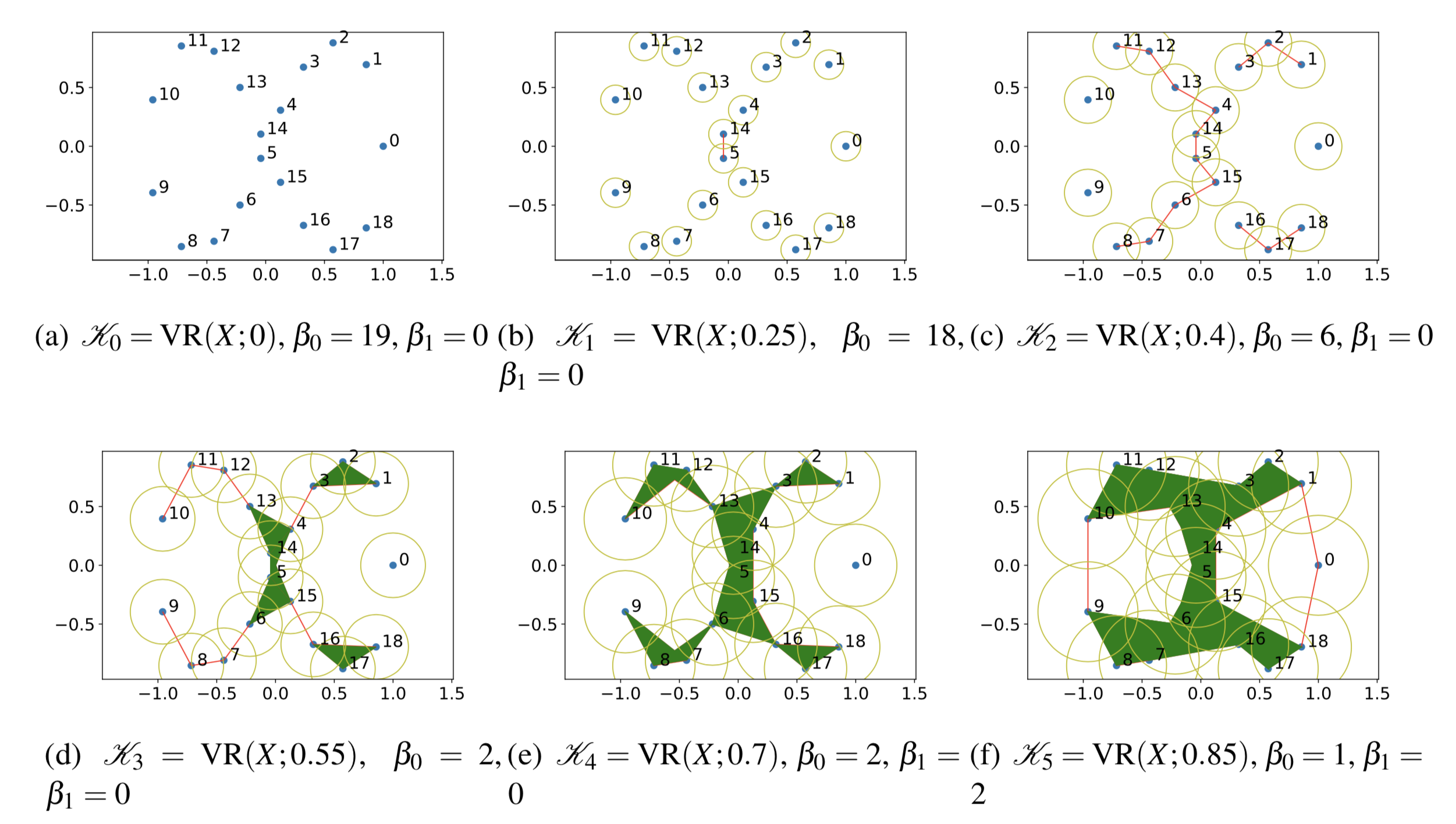
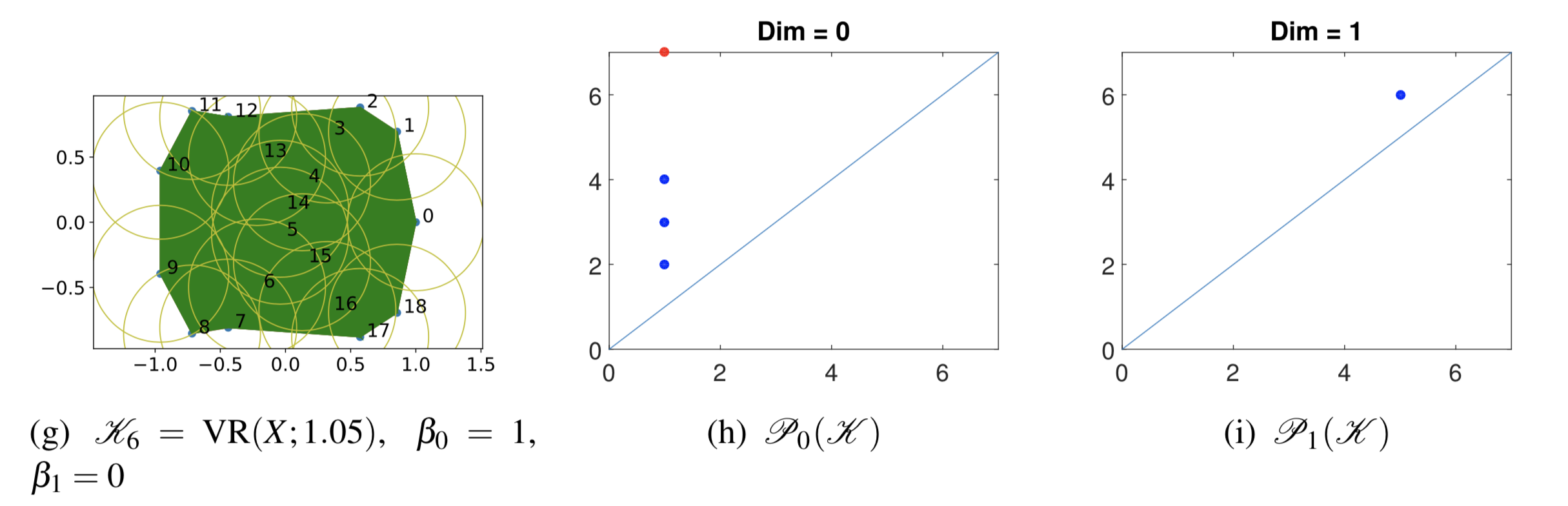
Figure SI.11. An example of filtration made by Vietoris-Rips complex. Labels of $x,y$ axes in $(a)\sim(c)$ are arbitrary units.

Appendix SI.2 Takens’ Lag Map

In this section, we provide a review of “recovering the manifold” underlying the one dimensional time series. Precisely, we discuss a set of theorems provided in [70] and an associated embedding algorithm in the time series framework. The algorithm is well-known as the Takens’ lag map or lag map, and has been extensively applied to many fields. In a nutshell, the recovered manifold is the phase space on which the dynamics lives that generates the time series. From now on, denote $M$ to be a $d$-dim compact manifold without boundary. For the sake of self-containedness, we recall the following definitions.

Definition 11 (Discrete time dynamics).

By a discrete time dynamics, we mean a diffeomorhism $\varphi:\,M\rightarrow M$ with the time evolution $i\mapsto\varphi^{i}(x_{0})$, $i\in\mathbb{N}$, where $x_{0}$ is the starting status.

Definition 12 (Continuous time dynamics).

By a continuous time dynamics, we mean a smooth vector field $X\in\Gamma(M)$ with the time evolution $t\mapsto\gamma_{t}(x_{0})$, where $\gamma_{t}$ is the integral curve with respect to $X$ via $x_{0}$.

To simplify the discussion, in both cases, we denote $\Phi_{t}(x_{0})$ to be the time evolution with time $t\in\mathbb{N}$ or $\mathbb{R}$ with the starting point $x_{0}$.

Definition 13 (Observed time series).

Let $\Phi_{t}(x_{0})$ be a dynamics on $M$. The observation is modeled as a function $f:\,M\rightarrow\mathbb{R}$ and the observed time series is $f(\Phi_{t}(x_{0}))$.

The question we have interest is that if we have an observed time series $f(\Phi_{t}(x_{0}))$, can we recover $M$ and/or the dynamics? The positive answer and the precise statements are provided in the following two theorems. The proof of these theorems can be found in [70].

Theorem SI.2.0.1 (discrete time dynamics).

For a pair $(\varphi,f)$, $\varphi:\,M^{d}\rightarrow M^{d}$ is the $C^{2}$-diffeomorphism and $f\in C^{2}$, it is generic that the map $\Psi:\,M\rightarrow\mathbb{R}^{2d+1}$ given by

$$\Psi:\,x\mapsto(f(x),\,f(\varphi(x)),\,f(\varphi^{2}(x))\ldots f(\varphi^{2d}(x)))^{T}\in\mathbb{R}^{2d+1}$$

is an embedding.

By generic, we mean an open dense subset of all possible pairs $(\varphi,f)$. We mention that the theorems hold for non-compact manifolds if $f$ is proper. These technical assumptions are practically assumed held for real world datasets.

Theorem SI.2.0.2 (Continuous time dynamics).

When $X\in C^{2}(\Gamma M)$ and $f\in C^{2}(M)$, it is generic that $\Psi:\,M\rightarrow\mathbb{R}^{2d+1}$ given by

$$\Psi:\,x\mapsto(f(x),\,f(\gamma_{1}(x)),\,f(\gamma_{2}(x))\ldots f(\gamma_{2d}(x)))^{T}\in\mathbb{R}^{2d+1}$$

is an embedding, where $\gamma_{t}(x)$ is the flow of $X$ of time $t$ via $x$.

These theorems tell us that we could embed the manifold into a $(2d+1)$ dimensional Euclidean space if we have access to all dynamical behaviors from all points on the manifold. However, in practice the above model and theorem cannot be applied directly. Indeed, for a given dynamical system, most of time we may only have one or few experiments that are sampled at discrete times; that is, we only have access to one or few $x\in M$. We thus ask the following question. Suppose we have the time series

$$\left\{f(\Phi_{\ell\alpha}(x))\right\}_{\ell=0}^{N}$$

as our dataset, where $x\in M$ is fixed and inaccessible to us, $\alpha>0$ is the sampling period, and $N\gg 1$ is the number of samples, what can we do? We first give the following definition.

Definition 14.

The positive limit set (PLS) of $x$ of a vector field $X\in C^{2}\left(\Gamma M\right)$ is defined as

$$L_{c}^{+}(x):=\left\{x^{\prime}\in M|\,\exists\,t_{i}\rightarrow\infty,\;t_{i}\in\mathbb{R}\text{ such that }\gamma_{t_{i}}(x)\rightarrow x^{\prime}\right\}$$

and the PLS of $x$ of a diffeomorphism $\varphi:\,M\rightarrow M$ is defined as

$$L_{d}^{+}(x):=\left\{x^{\prime}\in M|\,\exists\,n_{i}\in\mathbb{N}\rightarrow\infty,\text{ such that }\varphi^{n_{i}}\left(x\right)\rightarrow x^{\prime}\right\}.$$

It turns out that in this case, we should know whether under generic assumptions the topology and dynamics in the PLS of $x$ is determined by $\{f(\Phi_{\ell\alpha}(x))\}_{\ell=0}^{\infty}$. Precisely, we have the following theorem:

Theorem SI.2.0.3 (Continuous dynamics with 1 trajectory).

Fix $x\in M$. When $X\in C^{2}(\Gamma M)$ with flow $\gamma_{t}$ passing $x$, then there exists a residual subset $C_{X,x}\subset\mathbb{R}^{+}$ such that for all $\alpha\in C_{X,x}$ and diffeomorphism $\varphi:=\gamma_{\alpha}$, the PLS $L_{c}^{+}(x)$ for flow $\gamma_{t}$ and $L_{d}^{+}(x)$ for $\varphi$ are the same; that is, for all $\alpha\in C_{X,x}$ and for all $q\in L_{c}^{+}(p)$, there exists $n_{i}\in\mathbb{N}\rightarrow\infty$ such that $\varphi^{n_{i}}(x)\rightarrow q$.

This theorem leads to the following corollary, which is what we need to analyze the time series.

Corollary SI.2.0.4.

Take $x\in M$, a generic pair $X\in C^{2}(\Gamma M)$ and $f\in C^{2}(M)$, and $a\in\mathbb{R}^{+}$ satisfying generic conditions depending on $X$ and $x$. Denote the set

$$\mathcal{P}:=\left\{f(\gamma_{k\alpha}(x)),\,f(\gamma_{k\alpha}(x)),\ldots,f(\gamma_{(k+2d)\alpha}(x))\right\}_{k=0}^{\infty}.$$

Then there exists a smooth embedding of $M$ into $\mathbb{R}^{2d+1}$ mapping PLS $L_{c}^{+}$ bijectively to the set $\mathcal{P}$.

Last but not the least, we remark that the noise analysis of the Takens’ lag map has been extensively studied, for example [68].

Appendix SI.3 More Automatic Annotation Results

To further illustrate the robustness of our model and features, we perform more cross-database validation.

SI.3.1. Visualize features $\Phi^{(\texttt{PS})}(\mathcal{P}_{i}(R_{120,1}))$

The visualization of $\Phi^{(\texttt{PS})}(\mathcal{P}_{i}(R_{120,1}))$, where $i=0,1$, is shown in Figure SI.12. In order to compare them on the same scale, we perform the standard $z$-score normalization for each parameter in $\Phi^{(\texttt{PS})}(\mathcal{P}_{i}(R_{120,1}))$. We abuse the notation and use the same notation $\Phi^{(\texttt{PS})}(\mathcal{P}_{i}(R_{120,1}))$ to denote the normalized parameters. The boxplot of each normalized PS parameter, where blue (red) bars represent the PS associated with an IHR time series associated with the sleep (Wake) stage, is shown in Figure SI.12. We performed a rank sum test with a significance level of $0.05$ with the Bonferroni correction. We found that there are significant differences between waking and sleeping features for all PS parameters, except two parameters in $\Phi^{(\texttt{PS})}(\mathcal{P}_{0}(R_{120,1}))$. The first principal components of $\cup_{k}\{\Phi^{(\texttt{PS})}(\mathcal{P}_{i}(R_{120,1}))\}_{j=1}^{n_{k}}$ are shown in Figure SI.12(c) and (d). We can observe a separation between sleep and Wake features.

(a) Boxplot. $\mathcal{P}_{0}$.

(b) Boxplot plot. $\mathcal{P}_{1}$.

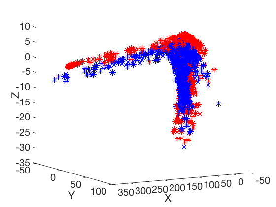
(c) Scatter plot. $\mathcal{P}_{0}$.

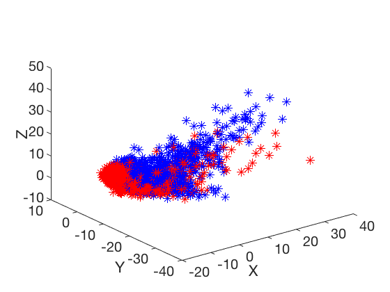
(d) Scatter plot. $\mathcal{P}_{1}$.

Figure SI.12. Distribution of normalized PS features, $\Phi^{(\texttt{PS})}(\mathcal{P}(R_{120,1}))$. (a)-(b) Boxplot of the $\Phi^{(\texttt{PS})}(\mathcal{P}_{i}(R_{120,1}))$ where $i=0$, $1$, respectively. The numbers listed on the horizontal axis indicates the number of PS. * indicates that the feature fails to reject the null hypothesis of the significance level of $0.05$ on the rank sum test with Bonferroni correction. (c)-(d) Visualization of $\cup_{k}\{\Phi^{(\texttt{PS})}(\mathcal{P}_{i}(R_{120,1}))\}_{j=1}^{n_{k}}$ by the first three principal components.

SI.3.2. For the classification of sleep and Wake

We consider the models trained on DREAMS and UCDSADB as shown in Table 4 and Table 5, respectively. In Table 4, we observe that the (SE, SP) pairs are consistent and all are located in the level of $(60,70)$ except for the UCDSADB. In Table 5, we also observe that the (SE, SP) pairs are all on the level of $(60,70)$. These consistent performances suggest that our proposed topological features, persistence statistics, are stable and well capture intrinsic characteristics about the sleep and Wake IHR signals.

Table 4. SVM cross-database performance of subjects for Wake and Sleep classification with a single random seed. The training database is DREAMS. For each database and each performance measurement, we report the mean $\pm$ standard deviation of all subjects.

CGMH-training CGMH-validation DREAMS UCDSADB TP 74 $\pm$ 43 72 $\pm$ 40 112 $\pm$ 57 86 $\pm$ 47 FP 166 $\pm$ 55 141 $\pm$ 54 176 $\pm$ 64 165 $\pm$ 63 TN 447 $\pm$ 69 434 $\pm$ 97 592 $\pm$ 112 431 $\pm$ 114 FN 29 $\pm$ 34 43 $\pm$ 44 45 $\pm$ 41 71 $\pm$ 54 SE $(\%)$ 75.9 $\pm$ 15.7 70.7 $\pm$ 17.0 73.7 $\pm$ 15.0 58.6 $\pm$ 16.9 SP $(\%)$ 73.5 $\pm$ 7.1 76.5 $\pm$ 6.3 77.6 $\pm$ 6.0 72.5 $\pm$ 7.1 Acc $(\%)$ 72.7 $\pm$ 6.7 73.6 $\pm$ 4.7 75.9 $\pm$ 5.3 68.7 $\pm$ 7.7 PR $(\%)$ 31.6 $\pm$ 18.3 35.9 $\pm$ 18.9 39.2 $\pm$ 18.1 33.6 $\pm$ 17.3 F1 0.411 $\pm$ 0.168 0.431 $\pm$ 0.129 0.481 $\pm$ 0.142 0.397 $\pm$ 0.149 AUC 0.810 $\pm$ 0.099 0.800 $\pm$ 0.101 0.825 $\pm$ 0.075 0.698 $\pm$ 0.125 Kappa 0.285 $\pm$ 0.155 0.291 $\pm$ 0.110 0.351 $\pm$ 0.142 0.215 $\pm$ 0.166

Table 5. SVM cross-database performance for Wake and Sleep classification. The training database is UCDSB database with a single random seed. For each database and each performance measurement, we report the mean $\pm$ standard deviation of all subjects.

CGMH-training CGMH-validation DREAMS UCDSADB TP 77 $\pm$ 45 77 $\pm$ 44 110 $\pm$ 63 99 $\pm$ 55 FP 192 $\pm$ 58 167 $\pm$ 60 232 $\pm$ 83 179 $\pm$ 67 TN 421 $\pm$ 62 409 $\pm$ 92 535 $\pm$ 98 417 $\pm$ 105 FN 25 $\pm$ 33 41 $\pm$ 44 47 $\pm$ 35 58 $\pm$ 44 SE $(\%)$ 79.6 $\pm$ 15.3 71.9 $\pm$ 17.8 70.4 $\pm$ 13.3 61.4 $\pm$ 18.8 SP $(\%)$ 69.3 $\pm$ 7.0 72.0 $\pm$ 6.5 70.5 $\pm$ 7.7 70.1 $\pm$ 6.2 Acc $(\%)$ 69.7 $\pm$ 6.8 70.2 $\pm$ 5.6 69.6 $\pm$ 6.7 68.2 $\pm$ 6.5 PR $(\%)$ 29.6 $\pm$ 17.7 32.8 $\pm$ 18.6 33.1 $\pm$ 19.0 34.4 $\pm$ 17.7 F1 0.398 $\pm$ 0.168 0.409 $\pm$ 0.149 0.420 $\pm$ 0.163 0.420 $\pm$ 0.170 AUC 0.815 $\pm$ 0.107 0.783 $\pm$ 0.120 0.771 $\pm$ 0.092 0.707 $\pm$ 0.113 Kappa 0.263 $\pm$ 0.156 0.255 $\pm$ 0.136 0.266 $\pm$ 0.161 0.241 $\pm$ 0.157

SI.3.3. For the classification of REM and NREM

We consider the models trained on DREAMS and UCDSADB for the REM and NREM classification. The results are summarized in Tables 6 and 7 respectively. We observe that the overall performance is consistent. As expected, the performance of the model trained on DREAMS is degraded on UCDSADB, and the performance of the model trained on UCDSADB on other databases is slightly lower, particularly the SE’s.

Table 6. SVM cross-database performance for REM and NREM classification. The training database is DREAMS with a single random seed. The subject $\#9$ in CGMH-validation and the subject $\#24$ in UCDSADB were dropped because they do not have REM epochs. For each database and each performance measurement, we report the mean $\pm$ standard deviation of all subjects.

CGMH-training CGMH-validation DREAMS UCDSADB TP 75 $\pm$ 31 68 $\pm$ 30 102 $\pm$ 32 65 $\pm$ 35 FP 130 $\pm$ 33 121 $\pm$ 47 155 $\pm$ 53 150 $\pm$ 34 TN 382 $\pm$ 66 376 $\pm$ 90 472 $\pm$ 94 356 $\pm$ 70 FN 25 $\pm$ 24 21 $\pm$ 16 37 $\pm$ 23 48 $\pm$ 36 SE $(\%)$ 76.8 $\pm$ 15.6 77.4 $\pm$ 16.7 74.8 $\pm$ 13.1 58.3 $\pm$ 18.0 SP $(\%)$ 74.6 $\pm$ 4.9 76.4 $\pm$ 6.4 75.6 $\pm$ 5.2 70.2 $\pm$ 6.1 Acc $(\%)$ 74.6 $\pm$ 6.0 75.3 $\pm$ 8.0 75.3 $\pm$ 5.9 67.8 $\pm$ 6.9 PR $(\%)$ 36.2 $\pm$ 12.4 38.1 $\pm$ 17.9 40.6 $\pm$ 12.2 29.5 $\pm$ 15.1 F1 0.479 $\pm$ 0.132 0.483 $\pm$ 0.155 0.519 $\pm$ 0.122 0.373 $\pm$ 0.155 AUC 0.823 $\pm$ 0.109 0.834 $\pm$ 0.109 0.819 $\pm$ 0.095 0.683 $\pm$ 0.131 Kappa 0.343 $\pm$ 0.145 0.353 $\pm$ 0.166 0.375 $\pm$ 0.147 0.197 $\pm$ 0.161

Table 7. SVM cross-database performance for REM and NREM classification. The training database is UCDSADB with a single random seed. The subject $\#9$ in CGMH-validation and the subject $\#24$ in UCDSADB were dropped because they do not have REM epochs. For each database and each performance measurement, we report the mean $\pm$ standard deviation of all subjects.

CGMH-training CGMH-validation DREAMS UCDSADB TP 60 $\pm$ 29 52 $\pm$ 23 75 $\pm$ 26 73 $\pm$ 40 FP 114 $\pm$ 32 108 $\pm$ 38 151 $\pm$ 45 117 $\pm$ 33 TN 398 $\pm$ 69 389 $\pm$ 93 478 $\pm$ 103 390 $\pm$ 70 FN 41 $\pm$ 25 36 $\pm$ 23 64 $\pm$ 32 41 $\pm$ 29 SE $(\%)$ 60.1 $\pm$ 17.9 60.3 $\pm$ 15.0 55.3 $\pm$ 15.5 65.3 $\pm$ 14.5 SP $(\%)$ 77.6 $\pm$ 5.0 78.1 $\pm$ 5.4 76.0 $\pm$ 4.5 76.9 $\pm$ 5.4 Acc $(\%)$ 74.6 $\pm$ 6.0 74.6 $\pm$ 9.0 72.0 $\pm$ 5.6 74.6 $\pm$ 5.9 PR $(\%)$ 33.8 $\pm$ 13.9 33.9 $\pm$ 14.5 33.6 $\pm$ 10.5 36.9 $\pm$ 16.2 F1 0.420 $\pm$ 0.143 0.412 $\pm$ 0.128 0.411 $\pm$ 0.115 0.452 $\pm$ 0.152 AUC 0.740 $\pm$ 0.135 0.742 $\pm$ 0.121 0.715 $\pm$ 0.113 0.773 $\pm$ 0.112 Kappa 0.278 $\pm$ 0.158 0.271 $\pm$ 0.146 0.244 $\pm$ 0.142 0.308 $\pm$ 0.152

SI.3.4. For the classification of Wake, REM and NREM

We consider the models trained on DREAMS and UCDSADB for the Wake, REM and NREM classification. The results are shown in Tables 8 and 9 respectively. We observe that the overall performances are consistent, and +P of NREM is higher than other classes as expected.

Table 8. SVM cross-database performance for Wake, REM and NREM classification. The training database is DREAMS with a single random seed. For each database and each performance measurement, we report the mean $\pm$ standard deviation of all subjects.

CGMH-training CGMH-validation DREAMS UCDSADB SE $(\%)$ (Wake) 63.3 $\pm$ 15.7 61.6 $\pm$ 17.7 64.8 $\pm$ 14.9 47.4 $\pm$ 14.7 SE $(\%)$ (REM) 54.7 $\pm$ 17.6 58.5 $\pm$ 19.0 59.4 $\pm$ 17.6 44.3 $\pm$ 17.6 SE $(\%)$ (NREM) 67.9 $\pm$ 9.3 69.3 $\pm$ 7.4 70.6 $\pm$ 8.2 61.3 $\pm$ 9.4 +P $(\%)$ (Wake) 34.7 $\pm$ 19.3 37.6 $\pm$ 16.4 44.6 $\pm$ 18.3 36.5 $\pm$ 17.5 +P $(\%)$ (REM) 37.3 $\pm$ 15.6 37.4 $\pm$ 18.0 42.4 $\pm$ 14.0 29.0 $\pm$ 16.5 +P $(\%)$ (NREM) 88.3 $\pm$ 8.7 85.5 $\pm$ 16.0 85.2 $\pm$ 7.8 75.9 $\pm$ 9.4 Acc $(\%)$ 64.5 $\pm$ 8.1 64.4 $\pm$ 8.3 66.9 $\pm$ 6.3 55.0 $\pm$ 8.5 Kappa 0.351 $\pm$ 0.116 0.346 $\pm$ 0.106 0.398 $\pm$ 0.104 0.227 $\pm$ 0.127

Table 9. SVM cross-database performance for Wake, REM and NREM classification. The training database is UCDSADB with a single random seed. For each database and each performance measurement, we report the mean $\pm$ standard deviation of all subjects.

CGMH-training CGMH-validation DREAMS UCDSADB SE $(\%)$ (Wake) 68.8 $\pm$ 17.0 61.3 $\pm$ 20.0 59.6 $\pm$ 15.8 53.6 $\pm$ 13.9 SE $(\%)$ (REM) 26.8 $\pm$ 13.4 27.8 $\pm$ 18.9 23.9 $\pm$ 14.0 39.6 $\pm$ 17.8 SE $(\%)$ (NREM) 76.0 $\pm$ 7.5 76.7 $\pm$ 6.9 76.3 $\pm$ 6.9 72.6 $\pm$ 7.0 +P $(\%)$ (Wake) 33.9 $\pm$ 18.6 34.1 $\pm$ 15.8 37.1 $\pm$ 20.7 39.3 $\pm$ 17.1 +P $(\%)$ (REM) 36.7 $\pm$ 21.1 34.5 $\pm$ 16.6 34.7 $\pm$ 17.0 46.3 $\pm$ 22.0 +P $(\%)$ (NREM) 86.4 $\pm$ 9.1 83.1 $\pm$ 16.0 81.2 $\pm$ 8.6 77.1 $\pm$ 8.4 Acc $(\%)$ 67.1 $\pm$ 7.2 65.5 $\pm$ 9.8 64.7 $\pm$ 6.2 63.6 $\pm$ 7.3 Kappa 0.343 $\pm$ 11.2 0.313 $\pm$ 0.105 0.311 $\pm$ 0.105 0.314 $\pm$ 0.125

SI.3.5. Subsampling effect

We further evaluate the impact of the subsampling process. We repeat all the above experiments with $20$ different random seeds. For each database, each performance measurement and each random seed, we record the mean of all subjects. Then we report the mean $\pm$ standard deviation of these $20$ results. Specifically, we take the random seeds $1\sim 20$ in MATLAB, which leads to $20$ different training datasets after the subsampling scheme. We observe that although subsampling process was utilized in the training procedure, the performance of each SVM model is stable in the sense that all performance measurements have small standard deviation below $1\%$. See Tables 10 to 18.

Table 10. SVM cross-database performance for Wake and Sleep classification. The training database is CGMH-training with 20 random seeds, $1\sim 20$; that is, we train 20 SVM models.

CGMH-training CGMH-validation DREAMS UCDSADB TP 6728 $\pm$ 26 2027 $\pm$ 14 2019 $\pm$ 10 2082 $\pm$ 17 FP 13200 $\pm$ 143 3360 $\pm$ 39 3456 $\pm$ 41 3679 $\pm$ 37 TN 41347 $\pm$ 143 12166 $\pm$ 39 11891 $\pm$ 41 11234 $\pm$ 37 FN 2423 $\pm$ 26 1149 $\pm$ 14 1119 $\pm$ 10 1850 $\pm$ 17 SE $(\%)$ 73.5 $\pm$ 0.3 63.8 $\pm$ 0.4 64.3 $\pm$ 0.3 53.0 $\pm$ 0.4 SP $(\%)$ 75.8 $\pm$ 0.3 78.4 $\pm$ 0.3 77.5 $\pm$ 0.3 75.3 $\pm$ 0.3 Acc $(\%)$ 75.5 $\pm$ 0.2 75.9 $\pm$ 0.2 75.3 $\pm$ 0.2 70.7 $\pm$ 0.1 PR $(\%)$ 33.8 $\pm$ 0.2 37.6 $\pm$ 0.2 36.9 $\pm$ 0.2 36.1 $\pm$ 0.1 F1 0.463 $\pm$ 0.001 0.474 $\pm$ 0.002 0.469 $\pm$ 0.002 0.430 $\pm$ 0.002 AUC 0.809 $\pm$ 0.000 0.781 $\pm$ 0.001 0.777 $\pm$ 0.001 0.693 $\pm$ 0.001 Kappa 0.331 $\pm$ 0.002 0.330 $\pm$ 0.002 0.323 $\pm$ 0.003 0.242 $\pm$ 0.002

Table 11. SVM cross-database performance for Wake and Sleep classification. The training database is DREAMS with 20 random seeds, $1\sim 20$; that is, we train 20 SVM models.

CGMH-training CGMH-validation DREAMS UCDSADB TP 6490 $\pm$ 49 1988 $\pm$ 16 2228 $\pm$ 13 2132 $\pm$ 23 FP 14590 $\pm$ 181 3730 $\pm$ 50 3458 $\pm$ 65 4128 $\pm$ 52 TN 39957 $\pm$ 181 11796 $\pm$ 50 11890 $\pm$ 65 10785 $\pm$ 52 FN 2660 $\pm$ 49 1189 $\pm$ 16 910 $\pm$ 13 1800 $\pm$ 23 SE $(\%)$ 70.9 $\pm$ 0.5 62.6 $\pm$ 0.5 71.0 $\pm$ 0.4 54.2 $\pm$ 0.6 SP $(\%)$ 73.3 $\pm$ 0.3 76.0 $\pm$ 0.3 77.5 $\pm$ 0.4 72.3 $\pm$ 0.4 Acc $(\%)$ 72.9 $\pm$ 0.2 76.4 $\pm$ 0.3 73.6 $\pm$ 0.3 68.5 $\pm$ 0.2 PR $(\%)$ 30.8 $\pm$ 0.2 34.8 $\pm$ 0.3 39.2 $\pm$ 0.4 34.1 $\pm$ 0.3 F1 0.429 $\pm$ 0.002 0.447 $\pm$ 0.003 0.505 $\pm$ 0.003 0.418 $\pm$ 0.003 AUC 0.781 $\pm$ 0.002 0.747 $\pm$ 0.003 0.808 $\pm$ 0.001 0.679 $\pm$ 0.002 Kappa 0.286 $\pm$ 0.002 0.293 $\pm$ 0.004 0.366 $\pm$ 0.004 0.218 $\pm$ 0.004

Table 12. SVM cross-database performance for Wake and Sleep classification. The training database is UCDSADB database with 20 random seeds, $1\sim 20$; that is, we train 20 SVM models.

CGMH-training CGMH-validation DREAMS UCDSADB TP 6814 $\pm$ 51 2050 $\pm$ 27 2176 $\pm$ 21 2464 $\pm$ 16 FP 16909 $\pm$ 219 4412 $\pm$ 67 4613 $\pm$ 62 4467 $\pm$ 54 TN 37638 $\pm$ 219 11114 $\pm$ 67 10734 $\pm$ 62 10445 $\pm$ 54 FN 2336 $\pm$ 51 1126 $\pm$ 27 962 $\pm$ 21 1468 $\pm$ 16 SE $(\%)$ 74.5 $\pm$ 0.6 64.6 $\pm$ 0.9 69.3 $\pm$ 0.7 62.7 $\pm$ 0.4 SP $(\%)$ 69.0 $\pm$ 0.4 71.6 $\pm$ 0.4 69.9 $\pm$ 0.4 70.1 $\pm$ 0.4 Acc $(\%)$ 69.8 $\pm$ 0.3 69.8 $\pm$ 0.3 68.7 $\pm$ 0.6 68.5 $\pm$ 0.2 PR $(\%)$ 28.7 $\pm$ 0.2 31.7 $\pm$ 0.3 32.1 $\pm$ 0.3 35.6 $\pm$ 0.2 F1 0.415 $\pm$ 0.002 0.425 $\pm$ 0.004 0.438 $\pm$ 0.003 0.454 $\pm$ 0.001 AUC 0.784 $\pm$ 0.002 0.733 $\pm$ 0.004 0.758 $\pm$ 0.003 0.716 $\pm$ 0.001 Kappa 0.261 $\pm$ 0.003 0.256 $\pm$ 0.005 0.269 $\pm$ 0.005 0.255 $\pm$ 0.002

Table 13. SVM cross-database performance for REM and NREM classification. The training database is CGMH-training with 20 random seeds, $1\sim 20$; that is, we train 20 SVM models.

CGMH-training CGMH-validation DREAMS UCDSADB TP 6731 $\pm$ 31 1776 $\pm$ 8 1877 $\pm$ 10 1558 $\pm$ 10 FP 10168 $\pm$ 98 2890 $\pm$ 39 2817 $\pm$ 35 3272 $\pm$ 40 TN 35446 $\pm$ 98 10338 $\pm$ 39 9749 $\pm$ 35 8921 $\pm$ 40 FN 2202 $\pm$ 31 522 $\pm$ 8 904 $\pm$ 10 1161 $\pm$ 10 SE $(\%)$ 75.4 $\pm$ 0.4 77.3 $\pm$ 0.4 67.5 $\pm$ 0.4 57.3 $\pm$ 0.4 SP $(\%)$ 77.7 $\pm$ 0.2 78.2 $\pm$ 0.3 77.6 $\pm$ 0.3 73.2 $\pm$ 0.3 Acc $(\%)$ 77.3 $\pm$ 0.1 75.8 $\pm$ 0.2 71.3 $\pm$ 0.3 70.3 $\pm$ 0.2 PR $(\%)$ 39.8 $\pm$ 0.1 38.1 $\pm$ 0.3 40.0 $\pm$ 0.2 32.3 $\pm$ 0.2 F1 0.521 $\pm$ 0.001 0.510 $\pm$ 0.003 0.502 $\pm$ 0.002 0.413 $\pm$ 0.002 AUC 0.836 $\pm$ 0.000 0.847 $\pm$ 0.001 0.796 $\pm$ 0.001 0.708 $\pm$ 0.001 Kappa 0.391 $\pm$ 0.001 0.389 $\pm$ 0.004 0.356 $\pm$ 0.003 0.234 $\pm$ 0.003

Table 14. SVM cross-database performance for REM and NREM classification. The training database is DREAMS database with 20 random seeds, $1\sim 20$; that is, we train 20 SVM models. .

CGMH-training CGMH-validation DREAMS UCDSADB TP 6608 $\pm$ 49 1747 $\pm$ 18 2020 $\pm$ 17 1533 $\pm$ 21 FP 11235 $\pm$ 216 3171 $\pm$ 66 3032 $\pm$ 68 3502 $\pm$ 66 TN 34379 $\pm$ 216 10057 $\pm$ 66 9534 $\pm$ 17 8692 $\pm$ 66 FN 2325 $\pm$ 49 551 $\pm$ 18 761 $\pm$ 17 1186 $\pm$ 21 SE $(\%)$ 74.0 $\pm$ 0.6 76.0 $\pm$ 0.8 72.6 $\pm$ 0.6 56.4 $\pm$ 0.8 SP $(\%)$ 75.4 $\pm$ 0.5 76.0 $\pm$ 0.5 75.9 $\pm$ 0.5 71.3 $\pm$ 0.5 Acc $(\%)$ 75.1 $\pm$ 0.3 76.0 $\pm$ 0.4 75.3 $\pm$ 0.4 68.6 $\pm$ 0.4 PR $(\%)$ 37.0 $\pm$ 0.3 35.5 $\pm$ 0.4 40.0 $\pm$ 0.4 30.5 $\pm$ 0.3 F1 0.494 $\pm$ 0.002 0.484 $\pm$ 0.005 0.516 $\pm$ 0.003 0.395 $\pm$ 0.004 AUC 0.815 $\pm$ 0.002 0.829 $\pm$ 0.006 0.816 $\pm$ 0.001 0.684 $\pm$ 0.004 Kappa 0.352 $\pm$ 0.004 0.354 $\pm$ 0.006 0.368 $\pm$ 0.004 0.208 $\pm$ 0.005

Table 15. SVM cross-database performance for REM and NREM classification. The training database is UCDSADB with 20 random seeds, $1\sim 20$; that is, we train 20 SVM models.

CGMH-training CGMH-validation DREAMS UCDSADB TP 5340 $\pm$ 77 1351 $\pm$ 23 1492 $\pm$ 24 1758 $\pm$ 19 FP 10351 $\pm$ 287 3044 $\pm$ 100 3368 $\pm$ 104 2869 $\pm$ 82 TN 35263 $\pm$ 287 9522 $\pm$ 100 9198 $\pm$ 104 9324 $\pm$ 82 FN 3593 $\pm$ 77 947 $\pm$ 23 1289 $\pm$ 24 961 $\pm$ 19 SE $(\%)$ 59.8 $\pm$ 0.9 58.8 $\pm$ 1.0 53.6 $\pm$ 0.9 64.7 $\pm$ 0.7 SP $(\%)$ 77.3 $\pm$ 0.6 77.3 $\pm$ 0.7 75.8 $\pm$ 0.8 76.5 $\pm$ 0.7 Acc $(\%)$ 74.4 $\pm$ 0.5 74.5 $\pm$ 0.6 71.8 $\pm$ 0.6 74.3 $\pm$ 0.4 PR $(\%)$ 34.0 $\pm$ 0.5 31.0 $\pm$ 0.7 40.8 $\pm$ 0.6 38.0 $\pm$ 0.5 F1 0.434 $\pm$ 0.004 0.406 $\pm$ 0.007 0.408 $\pm$ 0.005 0.479 $\pm$ 0.002 AUC 0.742 $\pm$ 0.005 0.733 $\pm$ 0.007 0.707 $\pm$ 0.006 0.771 $\pm$ 0.001 Kappa 0.284 $\pm$ 0.006 0.263 $\pm$ 0.009 0.236 $\pm$ 0.008 0.323 $\pm$ 0.004

Table 16. SVM cross-database performance for Wake, REM and NREM classification. The training database is CGMH-training with 20 random seeds, $1\sim 20$; that is, we train 20 SVM models.

CGMH-training CGMH-validation DREAMS UCDSADB SE $(\%)$ (Wake) 59.3 $\pm$ 0.2 53.4 $\pm$ 0.2 53.5 $\pm$ 0.2 37.3 $\pm$ 0.3 SE $(\%)$ (REM) 61.9 $\pm$ 0.2 65.2 $\pm$ 0.2 56.7 $\pm$ 0.4 47.7 $\pm$ 0.5 SE $(\%)$ (NREM) 71.3 $\pm$ 0.2 72.3 $\pm$ 0.3 71.5 $\pm$ 0.3 65.5 $\pm$ 0.4 +P $(\%)$ (Wake) 40.3 $\pm$ 0.1 45.3 $\pm$ 0.2 44.4 $\pm$ 0.1 38.2 $\pm$ 0.1 +P $(\%)$ (REM) 39.8 $\pm$ 0.2 37.4 $\pm$ 0.3 39.7 $\pm$ 0.2 28.0 $\pm$ 0.2 +P $(\%)$ (NREM) 89.5 $\pm$ 0.1 87.3 $\pm$ 0.1 83.7 $\pm$ 0.1 76.9 $\pm$ 0.1 Acc $(\%)$ 68.3 $\pm$ 0.1 68.2 $\pm$ 0.2 66.2 $\pm$ 0.1 57.0 $\pm$ 0.2 Kappa 0.402 $\pm$ 0.001 0.395 $\pm$ 0.002 0.372 $\pm$ 0.002 0.240 $\pm$ 0.001

Table 17. SVM cross-database performance for Wake, REM and NREM classification. The training database is DREAMS with 20 random seeds, $1\sim 20$; that is, we train 20 SVM models.

CGMH-training CGMH-validation DREAMS UCDSADB SE $(\%)$ (Wake) 60.1 $\pm$ 0.3 53.9 $\pm$ 0.4 62.9 $\pm$ 0.4 52.4 $\pm$ 0.4 SE $(\%)$ (REM) 53.8 $\pm$ 0.4 56.8 $\pm$ 0.5 57.9 $\pm$ 0.5 40.7 $\pm$ 0.6 SE $(\%)$ (NREM) 67.7 $\pm$ 0.3 69.6 $\pm$ 0.3 70.0 $\pm$ 0.3 72.5 $\pm$ 0.4 +P $(\%)$ (Wake) 33.9 $\pm$ 0.2 38.8 $\pm$ 0.2 44.6 $\pm$ 0.3 40.2 $\pm$ 0.2 +P $(\%)$ (REM) 37.8 $\pm$ 0.2 34.9 $\pm$ 0.3 42.8 $\pm$ 0.3 48.1 $\pm$ 0.6 +P $(\%)$ (NREM) 88.7 $\pm$ 0.1 87.3 $\pm$ 0.1 85.4 $\pm$ 0.1 77.5 $\pm$ 0.1 Acc $(\%)$ 64.6 $\pm$ 0.2 65.4 $\pm$ 0.2 67.0 $\pm$ 0.2 63.8 $\pm$ 0.2 Kappa 0.350 $\pm$ 0.002 0.354 $\pm$ 0.002 0.400 $\pm$ 0.002 0.321 $\pm$ 0.002

Table 18. SVM cross-database performance for Wake, REM and NREM classification. The training database is UCDSADB with 20 random seeds, $1\sim 20$; that is, we train 20 SVM models.

CGMH-training CGMH-validation DREAMS UCDSADB SE $(\%)$ (Wake) 63.7 $\pm$ 0.4 58.3 $\pm$ 0.5 47.1 $\pm$ 1.0 43.2 $\pm$ 0.9 SE $(\%)$ (REM) 26.9 $\pm$ 0.4 26.0 $\pm$ 0.5 22.7 $\pm$ 0.4 36.7 $\pm$ 0.6 SE $(\%)$ (NREM) 75.5 $\pm$ 0.3 77.0 $\pm$ 0.3 75.5 $\pm$ 0.3 70.8 $\pm$ 0.8 +P $(\%)$ (Wake) 33.0 $\pm$ 0.2 35.0 $\pm$ 0.3 36.0 $\pm$ 0.2 35.3 $\pm$ 0.3 +P $(\%)$ (REM) 38.5 $\pm$ 0.4 34.1 $\pm$ 0.5 35.6 $\pm$ 0.5 38.5 $\pm$ 0.2 +P $(\%)$ (NREM) 86.6 $\pm$ 0.1 84.7 $\pm$ 0.2 81.6 $\pm$ 0.1 75.4 $\pm$ 0.2 Acc $(\%)$ 67.0 $\pm$ 0.1 66.9 $\pm$ 0.2 64.6 $\pm$ 0.2 60.1 $\pm$ 0.3 Kappa 0.339 $\pm$ 0.002 0.322 $\pm$ 0.003 0.308 $\pm$ 0.002 0.253 $\pm$ 0.002

References

- [1] Henry Adams, Tegan Emerson, Michael Kirby, Rachel Neville, Chris Peterson, Patrick Shipman, Sofya Chepushtanova, Eric Hanson, Francis Motta, and Lori Ziegelmeier. Persistence images: A stable vector representation of persistent homology. The Journal of Machine Learning Research, 18(1):218–252, 2017.
- [2] Robert J Adler, Omer Bobrowski, Matthew S Borman, Eliran Subag, Shmuel Weinberger, et al. Persistent homology for random fields and complexes. In Borrowing strength: theory powering applications–a Festschrift for Lawrence D. Brown, pages 124–143. Institute of Mathematical Statistics, 2010.
- [3] M. Aktaruzzaman, M. Migliorini, M. Tenhunen, S. L. Himanen, a. M. Bianchi, and R. Sassi. The addition of entropy-based regularity parameters improves sleep stage classification based on heart rate variability. Med Biol Eng Comput, 53:415–425, 2015.
- [4] N Atienza, LM Escudero, MJ Jimenez, and M Soriano-Trigueros. Persistent entropy: a scale-invariant topological statistic for analyzing cell arrangements. arXiv preprint arXiv:1902.06467, 2019.
- [5] Nieves Atienza, Rocio Gonzalez-Diaz, and Matteo Rucco. Persistent entropy for separating topological features from noise in vietoris-rips complexes. J Intell Inf Syst, 52(3):637–655, 2019.
- [6] Nieves Atienza, Rocío González-Díaz, and M. Soriano-Trigueros. On the stability of persistent entropy and new summary functions for TDA. CoRR, abs/1803.08304, 2018.
- [7] Paul Bendich, Sang Peter Chin, Jesse Clark, Jonathan Desena, John Harer, Elizabeth Munch, Andrew Newman, David Porter, David Rouse, Nate Strawn, et al. Topological and statistical behavior classifiers for tracking applications. IEEE T Aero Elec Sys, 52(6):2644–2661, 2016.
- [8] Eric Berry, Yen-Chi Chen, Jessi Cisewski-Kehe, and Brittany Terese Fasy. Functional summaries of persistence diagrams. arXiv preprint arXiv:1804.01618, 2018.
- [9] R. B. Berry, D. G. Budhiraja, and et al. Rules for scoring respiratory events in sleep: update of the 2007 AASM manual for the scoring of sleep and associated events. J Clin Sleep Med, 8(5):597–619, 2012.
- [10] Silvia Biasotti, Leila De Floriani, Bianca Falcidieno, Patrizio Frosini, Daniela Giorgi, Claudia Landi, Laura Papaleo, and Michela Spagnuolo. Describing shapes by geometrical-topological properties of real functions. ACM Computing Surveys (CSUR), 40(4):12, 2008.
- [11] G. E. Billman. Heart rate variability–a historical perspective. Frontiers in physiology, 2:86, 2011.
- [12] Andrew J. Blumberg, Itamar Gal, Michael A. Mandell, and Matthew Pancia. Robust statistics, hypothesis testing, and confidence intervals for persistent homology on metric measure spaces. Found Comput Math, 14(4):745–789, Aug 2014.
- [13] Omer Bobrowski and Matthew Kahle. Topology of random geometric complexes: a survey. Journal of applied and Computational Topology, pages 1–34, 2018.
- [14] M. H. Bonnet and D. L. Arand. Heart rate variability: Sleep stage, time of night, and arousal influences. Electroencephalogr. Clin. Neurophysiol., 102(5):390–396, 1997.
- [15] Peter Bubenik. Statistical topological data analysis using persistence landscapes. The Journal of Machine Learning Research, 16(1):77–102, 2015.
- [16] Gunnar Carlsson. Topology and data. Bull. Amer. Math. Soc., 46(2):255–308, 2009.
- [17] Gunnar Carlsson, Afra Zomorodian, Anne Collins, and Leonidas J Guibas. Persistence barcodes for shapes. International Journal of Shape Modeling, 11(02):149–187, 2005.
- [18] F. Chazal, Vin de Silva, and S. Oudot. Persistence stability for geometric complexes. Geometriae Dedicata, 173:193–214, 2014.
- [19] Ilya Chevyrev, Vidit Nanda, and Harald Oberhauser. Persistence paths and signature features in topological data analysis. IEEE T Pattern Anal, 2018.
- [20] Harish Chintakunta, Thanos Gentimis, Rocio Gonzalez-Diaz, Maria-Jose Jimenez, and Hamid Krim. An entropy-based persistence barcode. Pattern Recognit., 48(2):391–401, 2015.
- [21] F. Chouchou and M. Desseilles. Heart rate variability: A tool to explore the sleeping brain? Frontiers in Neuroscience, 8:1–9, 2014.
- [22] Y. Chung, C. Hu, A. Lawson, and C. Smyth. Topological approaches to skin disease image analysis. In 2018 IEEE International Conference on Big Data (Big Data), pages 100–105, Dec 2018.
- [23] Yu-Min Chung and Austin Lawson. Persistence curves: A canonical framework for summarizing persistence diagrams. arXiv preprint arXiv:1904.07768, 2019.
- [24] David Cohen-Steiner, Herbert Edelsbrunner, and John Harer. Stability of persistence diagrams. Discrete & Computational Geometry, 37:103–120, 2007.
- [25] David Cohen-Steiner, Herbert Edelsbrunner, John Harer, and Yuriy Mileyko. Lipschitz functions have lp-stable persistence. Found Comput Math, 10(2):127–139, 2010.
- [26] H. R. Colten and B. M. Altevogt. Functional and economic impact of sleep loss and sleep-related disorders. In H. R. Colten and B. M. Altevogt, editors, Sleep Disorders and Sleep Deprivation: An Unmet Public Health Problem. 2006.
- [27] Madalena Costa, Ary L Goldberger, and C-K Peng. Multiscale entropy analysis of complex physiologic time series. Physical review letters, 89(6):068102, 2002.
- [28] Thomas G Dietterich and Ghulum Bakiri. Solving multiclass learning problems via error-correcting output codes. J Artif Intell Res, 2:263–286, 1994.
- [29] Adina E. Draghici and J. Andrew Taylor. The physiological basis and measurement of heart rate variability in humans. J. Physiol. Anthropol., 35(1):22, 2016.
- [30] H. Edelsbrunner and J. Harer. Computational topology. an introduction. Amer. Math. Soc., Providence, Rhode Island, 2010.
- [31] Herbert Edelsbrunner, David Letscher, and Afra Zomorodian. Topological persistence and simplification. In Proceedings 41st Annual Symposium on Foundations of Computer Science, pages 454–463. IEEE, 2000.
- [32] M. Elgendi. Fast QRS detection with an optimized knowledge-based method: Evaluation on 11 standard ecg databases. PLoS ONE, 8(9):e73557, 2013.
- [33] S. Elsenbruch, M.J. Harnish, and W.C. Orr. Heart Rate Variability During Waking and Sleep in Healthy Males and Females. Sleep, 22:1067–1071, 1999.
- [34] Charles Epstein, Gunnar Carlsson, and Herbert Edelsbrunner. Topological data analysis. Inverse Problems, 27(12):120201, 2011.
- [35] Brittany Terese Fasy, Fabrizio Lecci, Alessandro Rinaldo, Larry Wasserman, Sivaraman Balakrishnan, Aarti Singh, et al. Confidence sets for persistence diagrams. Ann. Stat., 42(6):2301–2339, 2014.
- [36] M. Gidea and Y. Katz. Topological data analysis of financial time series: Landscapes of crashes. Physica : A, 491:820–834, 2018.
- [37] L. Glass. Introduction to controversial topics in nonlinear science: Is the normal heart rate chaotic? Chaos, 19(2):028501, 2009.
- [38] A.L. Goldberger, L.A.N. Amaral, L. Glass, J.M. Hausdorff, P.Ch. Ivanov, R.G. Mark, J.E. Mietus, G.B. Moody, C.-K. Peng, and H.E. Stanley. Physiobank, physiotoolkit, and physionet: Components of a new research resource for complex physiologic signals. Circulation, 101(23):e215–e220, 2000.
- [39] Rocio Gonzalez-Diaz, Eduardo Paluzo-Hidalgo, and José F Quesada. Towards emotion recognition: A persistent entropy application. In International Workshop on Computational Topology in Image Context, pages 96–109. Springer, 2019.
- [40] Yasuaki Hiraoka, Tomoyuki Shirai, Khanh Duy Trinh, et al. Limit theorems for persistence diagrams. The Annals of Applied Probability, 28(5):2740–2780, 2018.
- [41] C. Iber, S. Ancoli-Isreal, A.L. Chesson Jr., and S.F. Quan. The AASM Manual for Scoring of Sleep and Associated Events-Rules: Terminology and Technical Specification. American Academy of Sleep Medicine, 2007.
- [42] Matthew Kahle. Topology of random simplicial complexes: a survey. AMS Contemp. Math, 620:201–222, 2014.
- [43] J.-E. Kang, M. M. Lim, R. J. Bateman, J. J. Lee, L. P. Smyth, J. R. Cirrito, N. Fujiki, S. Nishino, and D. M. Holtzman. Amyloid-b Dynamics are regulated by Orexin and the sleep-wake cycle. Science, 326(Nov 13):1005–1007, 2009.
- [44] A Karni, D Tanne, B S Rubenstein, J J Askenasy, and D Sagi. Dependence on REM sleep of overnight improvement of a perceptual skill. Science, 265(5172):679–682, 1994.
- [45] Michael Kerber, Dmitriy Morozov, and Arnur Nigmetov. Geometry helps to compare persistence diagrams. Journal of Experimental Algorithmics, 22:1–4, 2017.
- [46] Kwangho Kim, Jisu Kim, and Alessandro Rinaldo. Time series featurization via topological data analysis: an application to cryptocurrency trend forecasting. arXiv preprint arXiv:1812.02987, 2018.
- [47] Genki Kusano, Yasuaki Hiraoka, and Kenji Fukumizu. Persistence weighted gaussian kernel for topological data analysis. In International Conference on Machine Learning, pages 2004–2013, 2016.
- [48] A. Lewicke, E. Sazonov, M. J. Corwin, M. Neuman, and S. Schuckers. Sleep versus wake classification from heart rate variability using computational intelligence: Consideration of rejection in classification models. IEEE Trans. Biomed. Eng., 55(1):108–118, 2008.
- [49] X. Long, P. Fonseca, R. Haakma, R. M. Aarts, and J. Foussier. Time-frequency analysis of heart rate variability for sleep and wake classification. In BIBE, pages 85–90, Nov 2012.
- [50] John Malik, Yu-Lun Lo, and Hau-Tieng Wu. Sleep-wake classification via quantifying heart rate variability by convolutional neural network. Physiol Meas, 39(8):085004, 2018.
- [51] Norbert Marwan, Niels Wessel, Udo Meyerfeldt, Alexander Schirdewan, and Jürgen Kurths. Recurrence-plot-based measures of complexity and their application to heart-rate-variability data. Physical review E, 66(2):026702, 2002.
- [52] M.O. Mendez and M. Matteucci. Sleep staging from Heart Rate Variability: time-varying spectral features and Hidden Markov Models. International Journal of Biomedical Engineering and Technology, 3:246–263, 2010.
- [53] Yuriy Mileyko, Sayan Mukherjee, and John Harer. Probability measures on the space of persistence diagrams. Inverse Problems, 27(12):124007, 2011.
- [54] Konstantin Mischaikow, Thomas Wanner, et al. Topology-guided sampling of nonhomogeneous random processes. The Annals of Applied Probability, 20(3):1068–1097, 2010.
- [55] Khushboo Mittal and Shalabh Gupta. Topological characterization and early detaction of bifurcation and chaos in complex systems using persistent homology. Chaos, 27:051102 : 1–9, 2017.
- [56] James R. Munkres. Elements of Algebraic Topology. Westview Press, 1993.
- [57] Nina Otter, Mason A Porter, Ulrike Tillmann, Peter Grindrod, and Heather A Harrington. A roadmap for the computation of persistent homology. EPJ Data Science, 6(1):17, 2017.
- [58] Takashi Owada. Limit theorems for the sum of persistence barcodes. arXiv preprint arXiv:1604.04058, 2016.
- [59] Vic Patrangenaru, Peter Bubenik, Robert L. Paige, and Daniel Osborne. Challenges in topological object data analysis. Sankhya A, 2018.
- [60] T. Penzel, J. W. Kantelhardt, R. P. Bartsch, M. Riedl, J. F. Kraemer, N. Wessel, C. Garcia, M. Glos, I. Fietze, and C. Schöbel. Modulations of heart rate, ECG, and cardio-respiratory coupling observed in polysomnography. Frontiers in Physiology, 7:460, 2016.
- [61] S. M. Pincus and A. L. Goldberger. Physiological time-series analysis: what does regularity quantify? Am J Physiol Heart Circ Physiol, 266(4):H1643–1656, 1994.
- [62] Stephen W Porges. The polyvagal theory: new insights into adaptive reactions of the autonomic nervous system. Clev Clin J Med, 76(Suppl 2):S86, 2009.
- [63] Jan Reininghaus, Stefan Huber, Ulrich Bauer, and Roland Kwitt. A stable multi-scale kernel for topological machine learning. In Proceedings of the IEEE conference on computer vision and pattern recognition, pages 4741–4748, 2015.
- [64] Lee M. Seversky, Shelby Davis, and Matthew Berger. On time-series topological data analysis: New data and opportunities. Workshop paper on IEEE Conference on Computer Vision and Pattern Recognition, 2016.
- [65] F. Shaffer, R. McCraty, and C. L. Zerr. A healthy heart is not a metronome: an integrative review of the heart’s anatomy and heart rate variability. Frontiers in Psychology, 5:1040, 2014.
- [66] F. Snyder, J. A. Hobson, D. F. Morrison, and F. Goldfrank. Changes in respiration, heart rate, and systolic blood pressure in human sleep. J. Appl. Physiol., 19:417–422, 1964.
- [67] V. K. Somers, M. E. Dyken, A. L. Mark, and F. M. Abboud. Sympathetic-nerve activity during sleep in normal subjects. N. Engl. J. Med., 328:303–307, 1993.
- [68] J. Stark, D.S. Broomhead, M.E. Davies, and J. Huke. Takens embedding theorems for forced and stochastic systems. Nonlinear Analysis: Theory, Methods & Applications, 30(8):5303–5314, 1997.
- [69] A Stys and T Stys. Current clinical applications of heart rate variability. Clinical Cardiology, 21(10):719–724, 1998.
- [70] F. Takens. Detecting strange attractors in turbulence. In David Rand and Lai-Sang Young, editors, Dynamical Systems and Turbulence, volume 898 of Lecture Notes in Mathematics, pages 366–381. Springer Berlin Heidelberg, 1981.
- [71] Task Force of the European Society of Cardiology and others. Heart rate variability, standards of measurement, physiological interpretation, and clinical use. circulation, 93:1043–1065, 1996.
- [72] Julian F Thayer and Esther Sternberg. Beyond heart rate variability: vagal regulation of allostatic systems. Ann. N. Y. Acad. Sci., 1088(1):361–372, 2006.
- [73] L. Toscani, P. F. Gangemi, A. Parigi, R. Silipo, P. Ragghianti, E. Sirabella, M. Morelli, L. Bagnoli, R. Vergassola, and G. Zaccara. Human heart rate variability and sleep stages. Ital. J. Neurol. Sci., 17(6):437–439, 1996.
- [74] Katharine Turner, Yuriy Mileyko, Sayan Mukherjee, and John Harer. Fréchet means for distributions of persistence diagrams. Discrete Comput Geom, 52(1):44–70, Jul 2014.
- [75] Katharine Turner, Sayan Mukherjee, and Doug M Boyer. Persistent homology transform for modeling shapes and surfaces. Inf inference, 3(4):310–344, 2014.
- [76] L.C. Vanderlei, C.M. Pastre, R.A. Hoshi, T.D. Carvalho, and M.F. Godoy. Basic notions of heart rate variability and its clinical applicability. Rev. Bras. Cir. Cardiovasc., 24:205–217, 2009.
- [77] B. V. Vaughn, S. R. Quint, J. A. Messenheimer, and K. R. Robertson. Heart period variability in sleep. Electroencephalogr. Clin. Neurophysiol., 94(3):155–162, 1995.
- [78] Vinay Venkataraman, Karthikeyan Natesan Ramamurthy, and Pavan Turaga. Persistent homology of attractors for action recognition. IEEE International Conference on Image Processing, 2016.
- [79] José Vicente, Pablo Laguna, Ariadna Bartra, and Raquel Bailón. Drowsiness detection using heart rate variability. Med Biol Eng Comput, 54(6):927–937, 2016.
- [80] Andreas Voss, Steffen Schulz, Rico Schroeder, Mathias Baumert, and Pere Caminal. Methods derived from nonlinear dynamics for analysing heart rate variability. Philos. Trans. Royal Soc. A, 367(1887):277–296, 2008.
- [81] Yuan Wang, Hernando Ombao, and Moo K. Chung. Topological data analysis of single-trial electroencephalographic signals. Ann. Appl. Stat., 12(3):1506–1534, 09 2018.
- [82] M. Xiao, H. Yan, J. Song, Y. Yang, and X. Yang. Sleep stages classification based on heart rate variability and random forest. Biomed Signal Process Control, 8(6):624 – 633, 2013.
- [83] Y. Ye, K. Yang, J. Jiang, and B. Ge. Automatic sleep and wake classifier with heart rate and pulse oximetry: Derived dynamic time warping features and logistic model. In 10th Annu. Int. Syst. Conf. SysCon 2016 - Proc., pages 1–6, 2016.
- [84] D. Zemaityte and G. Varoneckas. Heart Rhythm Control During Sleep. Psychophysiology, 2(1972):279–290, 1984.
- [85] Bartosz Zielinski, Mateusz Juda, and Matthias Zeppelzauer. Persistence codebooks for topological data analysis. arXiv preprint arXiv:1802.04852, 2018.