Towards Assessing the Impact of Bayesian Optimization’s Own Hyperparameters

Abstract

Bayesian Optimization (BO) is a common approach for hyperparameter optimization (HPO) in automated machine learning. Although it is well-accepted that HPO is crucial to obtain well-performing machine learning models, tuning BO’s own hyperparameters is often neglected. In this paper, we empirically study the impact of optimizing BO’s own hyperparameters and the transferability of the found settings using a wide range of benchmarks, including artificial functions, HPO and HPO combined with neural architecture search. In particular, we show (i) that tuning can improve the any-time performance of different BO approaches, that optimized BO settings also perform well (ii) on similar problems and (iii) partially even on problems from other problem families, and (iv) which BO hyperparameters are most important.

1 Introduction

Due to its sample efficiency, Bayesian Optimization (BO) is a popular approach for optimizing the hyperparameters of machine learning algorithms Snoek et al. (2012); Bergstra et al. (2013); Thornton et al. (2013); Feurer et al. (2015); Jin et al. (2018); Shahriari et al. (2016); Feurer and Hutter (2019). Treating the validation loss of trained machine learning models as a black box function $f$, we can formulate the hyperparameter optimization problem as:

$$x^{*}\in\operatorname*{arg\,min}_{x\in\mathcal{X}}f(x)$$ (1)

where $\mathcal{X}$ is space of possible configurations $x$.

Although the community is aware of the necessity of hyperparameter optimization (HPO) for machine learning algorithms, the impact of BO’s own hyperparameters is not reported in most BO papers. On top of this, new BO approaches (and implicitly their hyperparameters) are often developed on cheap-to-evaluate artificial functions and then evaluated on real benchmarks. Although we acknowledge that this is a reasonable protocol to prevent over-engineering on the target function family (here for example HPO benchmarks of machine learning algorithms), we believe that it is important to study whether this practice is indeed well-founded.

We emphasize that this paper considers HPO on two levels as shown in Figure 1: (i) HPO of machine learning algorithms, which we consider as our target function (Target BO) and (ii) optimization of the target-BO’s own choices using a meta-optimizer.

Figure 1: Using a meta-optimizer to optimize the hyperparameters of a target Bayesian Optimization system, where $f$ is the target function, $s$ and $\lambda$ are a random seed and the hyperparameters of the target-BO.

In particular, we study several research questions related to the meta-optimization problem of BO’s hyperparameters:

1. How large is the impact of tuning BO’s own hyperparameters if one was allowed to tune these on each function independently?

2. How well does the performance of an optimized configuration of the target-BO generalize to similar new functions from the same family?

3. How well does the performance of an optimized configuration of the target-BO generalize to new functions from different families?

4. Which hyperparameters of the target-BO are actually important on the benchmarks considered and how does their best setting depend on the benchmark family being considered?

To answer these questions, we ran extensive empirical studies on different function families, including commonly used artificial functions, hyperparameter optimization on Support Vector Machines (SVMs), and hyperparameter optimization and architecture search for (small-scale) deep neural networks. Since applying BO for HPO is already expensive, meta-optimization of BO’s hyperparameters can easily become infeasible. Therefore, we surrogate HPO benchmarks Eggensperger et al. (2015, 2018), as recently widely adopted in the BO-community Falkner et al. (2018); Perrone et al. (2018); Probst et al. (2019).

2 Background: Bayesian Optimization

Input : Search Space $\mathcal{X}$, black box function $f$, acquisition function $\alpha$, maximal number of function evaluations $m$

1 $\mathcal{D}_{0}$ $\leftarrow$ initial_design($\mathcal{X}$);

2 for n = $1,2,\ldots m-|D_{0}|$ do

3       $\hat{f}$ $\leftarrow$ fit predictive model on $\mathcal{D}_{n-1}$;

4       select $x_{n}$ by optimizing $x_{n}\in\operatorname*{arg\,max}_{x\in\mathcal{X}}\alpha(x;\mathcal{D}_{n-1},\hat{f})$;

5       Query $y_{n}:=f(x_{n})$;

6       Add observation to data $D_{n}:=D_{n-1}\cup\{\langle x_{n},y_{n}\rangle\}$;

7      

return Best seen $x$

Algorithm 1 Bayesian Optimization (BO)

Bayesian Optimization (BO) aims to minimize the number of function evaluations required to minimize black box function. To this end, a predictive model $\hat{f}$ is trained on all pairs $\langle x,f(x)\rangle$ of points observed so far to estimate the unknown function $f$. Gaussian Processes (GPs) are a common choice to model $\hat{f}$, due to their closed-form tractability and their well-calibrated uncertainty estimates. Alternatives to GPs include random forests (RFs)  Hutter et al. (2011) and artificial neural networks Snoek et al. (2015); Springenberg et al. (2016); Perrone et al. (2018); however, these are rare since obtaining efficient out-of-the-box uncertainty estimates in DNNs is still a topic of ongoing research.

Bayesian Optimization is shown in Algorithm 1. It starts with using an initial design to sample the search space $\mathcal{X}$. In the simplest case, this can be a single, randomly drawn point $x_{0}$ and its corresponding function value $f(x_{0})$. The initial design gives rise to initial observation data $D_{0}:=\{\langle x_{i},f(x_{i})\rangle\}_{i}$. Given the remaining budget of function evaluations (or other budgets such as time constraints), BO iterates the following three steps: (i) it fits a probabilistic model $\hat{f}$ (typically a GP) to the previous observations $D_{n-1}$, (ii) it optimizes an acquisition function $\alpha$, trading off exploration and exploitation, to select the next point $x_{n}$, (iii) it queries $x_{n}$ to obtain $f(x_{n})$ and adds it to $D_{n-1}$. In the end, the algorithm typically returns the best seen $x$, the so-called incumbent.

To select the next point in each iteration, different acquisition functions can be optimized. A well known acquisition function is the expected improvement (EI) criterion Mockus et al. (1978). An advantage of EI is that it has a closed-form solution making it efficient to compute:

$$E[I(x)] =\mathbb{E}[\max\{0,f^{*}-f(x)\}]$$ (2)

$$=\sigma_{x}\cdot[u\cdot\Phi(u)+\phi(u)]$$

where $u:=\frac{f^{*}-\mu_{x}}{\sigma_{x}}$, $\mu_{x}$ and $\sigma_{x}$ are the mean and variance predicted by $\hat{f}$, $f^{*}$ is the best function value observed so far, and $\phi$ and $\Phi$ are the PDF and CDF of a normal distribution, resp. For an overview on BO and other acquisition functions, we refer the interested reader to recent overview papers Brochu et al. (2010); Shahriari et al. (2016); Frazier (2018).

3 Related Work

Already Jones et al. Jones et al. (1998) pointed out that the performance of global optimization algorithms can be improved by considering several design decisions; for example, they recommended to use different transformations of the response values to improve the performance of BO. Similar studies for example by Brockhoff et al. Brockhoff et al. (2015) and Morar et al. Morar et al. (2017) evaluated the impact of the initial design, while Picheny et al. Picheny et al. (2013) evaluated different acquisition functions for noisy benchmark problems.

Snoek et al. Snoek et al. (2015) used HPO to tune the architecture of the DNN in their DNGO approach, but they did not report the impact of their HPO and on which functions they exactly evaluated it. Given the importance of a good DNN architecture and its hyperparameter configuration, we expect that their HPO was crucial to achieve good performance.

Dang et al. Dang et al. (2017) performed a study similar to ours, but they studied how well surrogate benchmarks can be used for meta-tuning the algorithm configurator irace. In contrast to Dang et al, we focus here on BO and the problem of generalization of tuned BO configurations to other functions. Furthermore, we do not claim that surrogate benchmarks are a perfect replacement for real benchmarks functions, but we use them to approximate real-world problem with different surfaces to better understand the tunability of BO.

Slightly related to our study here are also recent efforts of automating design decisions of BO Hoffman et al. (2011); Grosse et al. (2012); Duvenaud et al. (2014); Malkomes et al. (2016), most of the time related to better predictive models. For example, Malkomes and Garnett Malkomes and Garnett (2018) proposed to use BO inside of the BO algorithm to improve the quality of the predictive model. Our work is orthogonal to theirs since they aim to locally improve the performance of a BO algorithm whereas we try to provide insights on the impact of BO’s own hyperparameters.

4 Hyperparameter Optimization for
Bayesian Optimization

To optimize the hyperparameters of the target-BO, we first need to define the loss metric to be optimized by the meta-optimizer. Because hitting the optimum as accurately as possible is important in many BO applications, we consider log-regret to the actual optimum of the target function. Although the optimum is not known in many applications, for the sake of our empirical study we assume that the optimum is given for the functions we used for training. The target-BO does not have access to the optimum and can only observe $f(x)$; the log-regret is only used for the meta-optimizer.

Another important characteristic of BO is a good anytime performance. Work on learning to learn Chen et al. (2017) and learning to optimize Li and Malik (2017) has shown that the performance over time yields a stronger signal than only considering the end point of an optimization trajectory. Therefore, we consider the log-regret averaged over time.

We also take into account that a robust BO approach should not only perform well on a single function, but at least on a family of similar functions, e.g., optimizing the hyperparameters of one algorithm on different datasets. Therefore, we are interested in optimizing the loss in expectation over a distribution of functions.

This leads us to the following meta-loss of our target-BO optimized by the meta-optimizer:

$$\mathcal{L}(\lambda)=\mathbb{E}_{f\sim\mathcal{F}}\left[\frac{1}{T}\sum_{t=1}^{T}\min_{\hat{x}\in\mathbf{x}(\lambda)_{1:t}}\log\left(f(\hat{x})-f(x^{*})\right)\right]$$ (3)

where $\mathcal{F}$ is a distribution over functions $f$, $x^{*}$ is the optimum of $f$, $T$ is the budget of allowed function evaluations and $\lambda$ is a hyperparameter configuration of the target-BO used to obtain a sequence of samples $\mathbf{x}_{1:t}$ (one for each time step).

4.1 Meta-Optimization

Our meta-optimization problem itself is a hyperparameter optimization problem. A straightforward approach would be to apply BO as meta-optimizer to tune the target-BO Snoek et al. (2015). However, since we are interested in a configuration $\lambda^{*}$ that performs well across a set of functions, we would need to evaluate the target-BO for each configuration $\lambda$ on all functions (if we can assume that we approximate the distribution of functions by a finite set of functions). Even if the target functions would be fairly cheap (e.g., artificial functions such as Branin), the meta-optimization would be very expensive because of the overhead induced by BO, i.e., predictive model training and acquisition function optimization.

To efficiently optimize our loss $\mathcal{L}(\lambda)$, we use approaches from algorithm configuration. As recently argued by Eggensperger et al. Eggensperger et al. (2018), algorithm configuration is a variant of hyperparameter optimization. Algorithm configuration aims to minimize an algorithm’s cost $c(\lambda,\pi)$ w.r.t. a hyperparameter configuration $\lambda$ across a set of so-called instances $\pi\sim\Pi$:

$$\lambda^{*}\in\operatorname*{arg\,min}_{\lambda\in\Lambda}\mathbb{E}_{\pi\sim\Pi}\left[c(\lambda,\pi)\right]$$ (4)

By instantiating instances $\pi$ with functions $f$, we can directly apply this formulation to attack our optimization problem given in Equation 3.

4.2 Hyperparameters in Bayesian Optimization

Bayesian Optimization has many hyperparameters and design options. These include but are not limited to: the initial design (e.g., a Sobol sequence Snoek et al. (2012), random points Hutter et al. (2011), or latin-hypercube design Brockhoff et al. (2015)), the acquisition function (e.g., probability of improvement Kushner (1964), expected improvement Mockus et al. (1978) or upper confidence bounds Srinivas et al. (2010)), transformations of function value observations Jones et al. (1998), the predictive model and its hyperparameters (e.g., GPs or RFs Hutter et al. (2011)), and sometimes even interleaved random sampling is used Bull (2011); Hutter et al. (2011); Ahmed et al. (2016).

Based on these design options, we created three design spaces. To allow for a comprehensive and still manageable study, each of these spaces includes exactly one predictive model family and its hyperparameters: GP with maximum likelihood (GP-ML) Jones et al. (1998), with maximum a posteriori (GP-MAP) Snoek et al. (2012) and random forests (RF) Hutter et al. (2011). Although random forests are much less commonly used compared to GPs for BO, we included them here to study a complementary approach. Our BO-implementation and its default settings are inspired by the BO-tools Spearmint Snoek et al. (2012), RoBO Klein et al. (2017), GpyOpt The GPyOpt authors (2016) and SMAC Hutter et al. (2011). We note that all our models can handle continuous, categorical and conditional search spaces either natively (RF) or by using specialized kernels (GP) Lévesque et al. (2017). All three design spaces cover the initial design, the acquisition function, function value transformations and interleaved random sampling.

5 Experiments

We now discuss the results of studying the research questions presented in Section 1.

Family	#Functions	#Cont.	#Cat.	Conditionals	Ref.
Artificial functions	$10$	$2-6$	$0$	$\times$	–
HPO SVM	$10$	$3$	$1$	$\checkmark$	Kühn et al. (2018)
HPO+NAS ParamNet	$6$	$6$	$0$	$\times$	Falkner et al. (2018)

Table 1: Benchmarks from HPOlib with the family name, the number of benchmarks in each family, the number of continuous hyperparameters, the number of categorical hyperparameters, whether conditional dependencies between hyperparameters exist and a reference.

5.1 Experimental Setup

As function families, we chose three different, but fairly typical benchmarks for BO, see Table 1 First, we used commonly used artificial functions, including Branin or Hartmann3. These functions are continuous and have 2 to 6 dimensions. Second, we used benchmarks from an experimental study by Kühn et al. Kühn et al. (2018) for optimizing the hyperparameters of SVMs on 10 different datasets from OpenML. In contrast to the artificial functions, there is one categorical hyperparameter for choosing the kernel and two of the continuous hyperparameters are only active based on the chosen kernel. Third, we used benchmarks for optimizing small neural networks (including their architecture size, dropout rate, batchsize and learning rate). The latter two benchmarks are surrogate benchmarks Eggensperger et al. (2015) and thus we can fairly well approximate their optima.

We ran all benchmarks on a high-performance cluster equipped with Intel Xeon E5-2630v4 processors and 128GB RAM. We let the target-BO evaluate $100$ function evaluations to obtain a loss value for the meta-optimizer. As a meta-optimizer we chose to use SMACv3 Lindauer et al. (2017) and used a maximum runtime of 2 days to ensure that the meta-optimization can collect sufficient amounts of data. We ran the meta-optimizer 20 times with different random seeds whereas the first 10 runs used the standard SMAC mode and the second 10 runs used the random sampling of SMAC. We validated the best target-BO configuration found overall, by running it again on each function 20 times with different random seeds. In the following, we report aggregated results across all functions in a family.

5.2 Q1: Impact of Hyperparameter Optimization for Bayesian Optimization

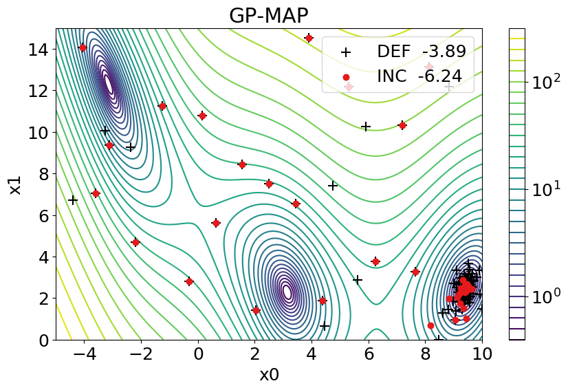
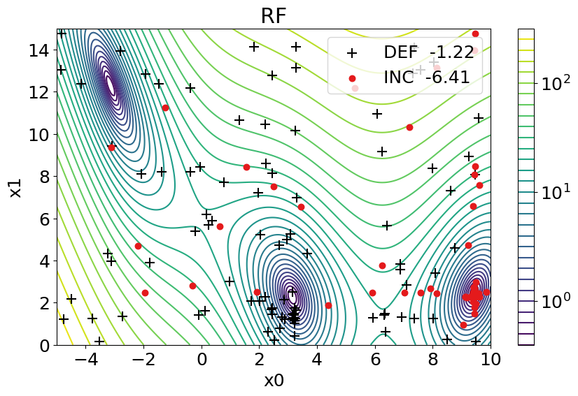
Figure 2: Sampling behavior of BO with GP-MAP (left) and RF (right) on the function Branin, including the samples of the default configurations (”DEF”) and the tuned incumbent configurations (”INC”). The final log-regret is shown in the legend.

	DEF	LOFO	ALL	IND	DEF	LOFO	ALL	IND	DEF	LOFO	ALL	IND
	RF				GP-ML				GP-MAP
artificial	$-0.19$	$\mathbf{-0.95}$	$\mathbf{-1.52}$	$\mathbf{-2.44}$	$-2.35$	$-2.50$	$\mathbf{-2.80}$	$\mathbf{-3.40}$	$-2.41$	$-2.43$	$\mathbf{-2.88}$	$\mathbf{-3.73}$
SVM	$-2.65$	$-2.73$	$\mathbf{-2.91}$	$\mathbf{-3.22}$	$-2.90$	$\mathbf{-3.11}$	$\mathbf{-3.10}$	$\mathbf{-3.36}$	$-2.87$	$-2.87$	$\mathbf{-3.08}$	$\mathbf{-3.40}$
ParamNet	$-2.12$	$\mathbf{-2.37}$	$\mathbf{-2.39}$	$\mathbf{-2.43}$	$-2.15$	$\mathbf{-2.36}$	$\mathbf{-2.39}$	$\mathbf{-2.47}$	$-2.25$	$\mathbf{-2.32}$	$\mathbf{-2.36}$	$\mathbf{-2.40}$

Table 2: Log-regret averaged over time across several target functions and 20 repetitions in each benchmark family. ”DEF” refers to the default setting, ”LOFO” to a leave-one-function-out setting within one family, ”ALL” to tuning on all functions within a family jointly, and ”IND” to tuning each function independently. We note that only in the ”LOFO” the optimized BO configuration has to generalize to new functions. setting We highlight results which perform significantly better than the default setting across the target functions using a paired, one-sided Wilcoxon signed rank test with a significance level of $0.05$.

	artificial	SVM	ParamNet	artificial	SVM	ParamNet	artificial	SVM	ParamNet
	RF			GP-ML			GP-MAP
artificial	$-0.95$	$-0.79$	$-0.91$	$-2.50$	$-2.65$	$-2.10^{*}$	$-2.43$	$-2.19^{*}$	$-2.40^{*}$
SVM	$-2.62^{*}$	$-2.73$	$-2.54^{*}$	$-3.01$	$-3.11$	$-2.93$	$-2.76^{*}$	$-2.87$	$-3.06$
ParamNet	$\mathbf{-2.30}$	$\mathbf{-2.27}$	$-2.37$	$-2.35$	$\mathbf{-2.32}$	$-2.36$	$-2.37$	$-2.34$	$-2.32$

Table 3: Log-regret averaged over time for the out-of-family setting. The columns refer to the function family used for the meta-optimization and the rows refer to the family the best configuration was applied to. Thus, we compare the numbers in each row. The diagonal refers to the setting where we tune in a leave-one-function-out setting and evaluate on the remaining function. Results are highlighted if the performance is significantly worse than the diagonal using a paired, one-sided Wilcoxon signed rank test with a significance level of $0.05$. We marked all results with a star^∗ if the performance is worse than the used default setting (as shown in Table 2).

Table 2 shows the results for each function family and each predictive model family. To discuss the impact of hyperparameter optimization on BO’s own hyperparameters, we compare columns ”DEF” (the default hyperparameter configuration; see Section 4.2), ”LOFO” (tuning jointly on all except one function from the family under consideration) , ”ALL” (tuning jointly on all functions of the family under consideration) and ”IND” (tuning the target-BO on each function independently). For each combination of function family, tuning setup and model, the performance of the tuned target-BO (”IND”) improved substantially over the default-BO (”DEF”), showing the importance of tuning BO’s own hyperparameters. We also observe slightly different rankings comparing models before and after tuning, which underlines the importance of tuning for fair comparisons of approaches.

Furthermore, we studied the sampling behavior of the BO approaches in detail, see Figure 2. On the well known benchmark function Branin, we can observe that all default configurations do far too much exploration by covering a lot of the space. However, the tuned configurations are much more greedy and exploit one of the optima much better. Since Branin has no local optima, this is an efficient strategy.

5.3 Q2: Generalization within Benchmark Families

To study generalization within a benchmark family, we run our meta-optimizer in a leave-one-function-out (LOFO) scheme, i.e., tuning the target BO on $n-1$ functions and evaluating it on the remaining one. The comparison of columns ”DEF” and ”LOFO” in Table 2 shows that it is indeed possible to tune BO’s own hyperparameter on similar functions from the same function family. In 5 out of 9 cases, the performance is significantly better than the default settings, but a bit worse than tuning on all functions from the same family (”ALL”) or on each function independently (”IND”). The latter also shows that tuning on each function comes with the risk of over-tuning a BO approach to a single function.

5.4 Q3: Generalization to New Benchmark Families

In Table 3, we show how well a tuned target-BO configuration performs on a different function family. We note that all our three function families are similar to some degree. The artificial functions and the ParamNet families are both low-dimensional, continuous functions; however, the ParamNet functions have a much smaller range of possible function values. Although the SVM family also has only a few dimensions, it is the only family (we considered) that has a categorical hyperparameter and conditional dependencies.

To our surprise, out-of-family tuning led to much better results than we expected. Most results are better than the default performance (as shown in Table 2). However, some results related to the SVM benchmarks show some potential issues for generalizing to new benchmark families, since it is our only family with categorical hyperparameters. Nevertheless, the results also show that the performance often drops significantly (although not always substantially) compared to optimizing on the same benchmark family. In some few cases, tuning on a different family actually led to a slightly better performance than tuning on the original family, e.g., tuning the GP-MAP on the SVM functions and applying the tuned configuration to the ParamNet functions. This is quite surprising because intuitively we expected that tuning on functions from the same family leads to the best results.

5.5 Q4: Most Important Hyperparameters

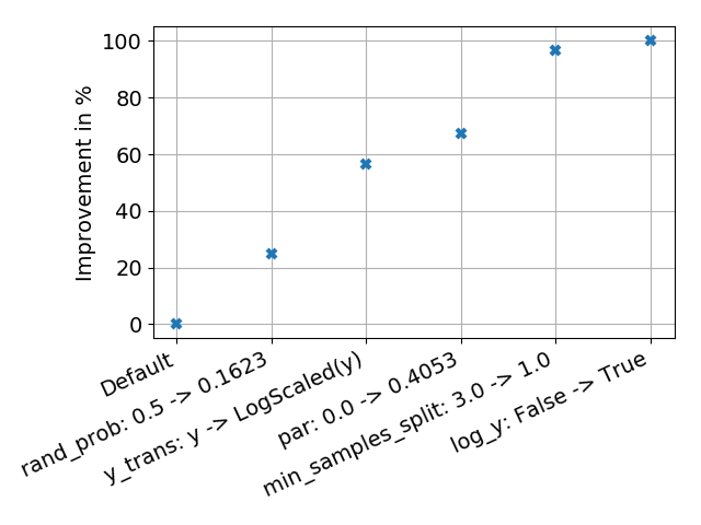
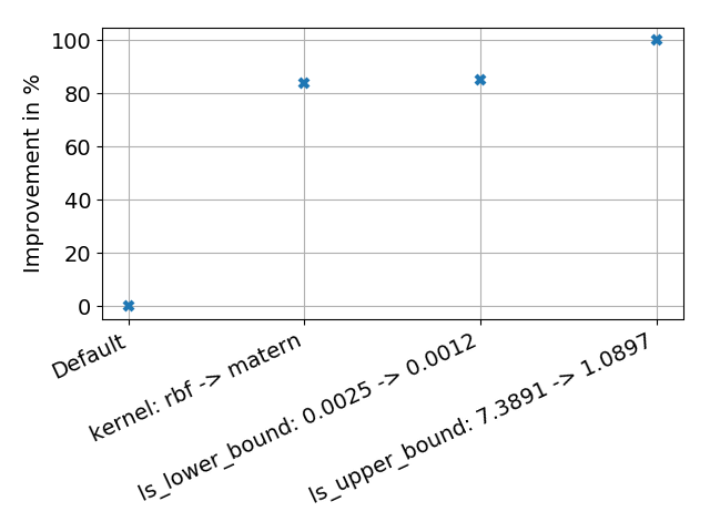
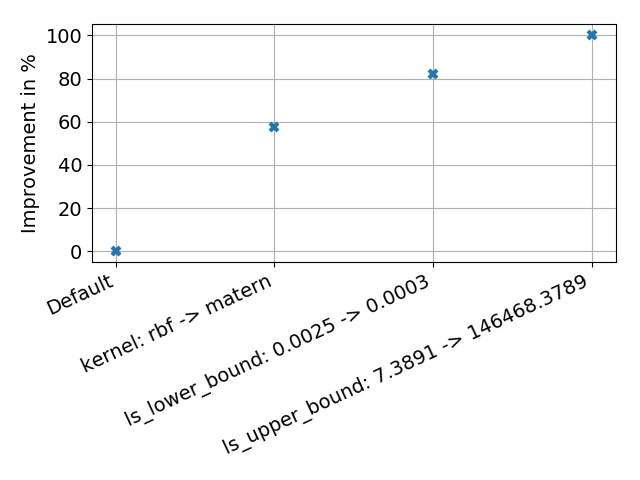
Figure 3: Results of an ablation study for RF (top), GP-ML (middle) and GP-MAP (bottom) to show which hyperparameters had to be tuned to achieve better performance on the artificial functions. An improvement of $0.0$ refers to the default performance and $1.0$ to the performance after tuning. Higher values are improvements over the configuration obtained during the tuning procedure. The x-axis shows at most $10$ hyperparameter changes which were in all cases sufficient to identify the most important hyperparameters. We show the ablation path from the default configuration to the best configuration found by tuning jointly on all functions from a family (corresponds to ”ALL” in Table 2).

To provide more insights which hyperparameters should actually be tuned, we ran an ablation study Fawcett and Hoos (2016). Starting from the default hyperparameter configuration and moving towards the best found configuration, this analysis iterates several times over all hyperparameters, and in each iteration, it greedily changes the most important hyperparameters from the default to its optimized setting.

Figure 3 shows three exemplary results of this study on the artificial functions. First, we note that not all of the tuned hyperparameters, but only a small set is important to improve performance. For the artificial functions these were always less than 6. Second, we observed that the important hyperparameters strongly depend on the used predictive model and also somewhat on the tuned function family. For example, for RFs, a smaller probability of interleaved random samples (rand_prob; default was $50\%$, now $16\%$), a transformation of the observed function values (y_trans) and a shift correction of the incumbent value (par) were important. For GP-MAP and GP-ML, the choice of the kernel (using a Matérn kernel instead of a RBF kernel) and the bounds for the hyperpriors of the length-scale (ls_lower_bound and ls_upper_bound) were important.

6 Conclusion and Future Work

We believe that this work is an important first step towards hyperparameter optimization of Bayesian Optimization, showing potential and limitations, and provides guidance which hyperparameters have to be tuned. In all our experiments, including three different predictive models on three different function families, the clear conclusion was that hyperparameter optimization is important and the default hyperparameter configurations we derived from well known tools leave ample room for improvement.

We showed that hyperparameter optimization of Bayesian Optimization is in fact possible in a leave-one-function-out manner, indicating that hyperparameter optimization can be jointly conducted on similar functions and applied to new functions from the same family. Even tuning on a different family of functions often worked surprisingly well, but it also comes with some risks. We expect that it is possible to construct function families that are quite different such that hyperparameter optimization will not generalize to new function families, e.g., the best BO setting for discrete functions with many categorical hyperparameters will most likely not resemble those for continuous, low-dimensional functions. In future work, we will study under which characteristics of the functions this generalization to new functions will fail.

Although our results show the importance of tuning the hyperparameters of Bayesian Optimization, our empirical study is based on assumptions that do not hold in most practical applications: (i) the optimum of the function is known and (ii) the target-function is cheap-to-evaluate. Therefore, in future work we will develop a practical approach, which does not require these assumptions. Since Bayesian Optimization is an iterative any-time algorithm, multi-fidelity optimization Falkner et al. (2018) will be a promising direction. Another idea for future work is to combine simulated function evaluations based on surrogate models with interleaved real HPO function evaluations, following a recent combination of simulated function evaluations and physical experiments Marco et al. (2017).

Acknowledgments

The authors acknowledge funding by the Robert Bosch GmbH, support by the state of Baden-Württemberg through bwHPC and the German Research Foundation (DFG) through grant no. INST 39/963-1 FUGG.

References

- Ahmed et al. [2016] M. Ahmed, B. Shahriari, and M. Schmidt. Do we need “harmless” Bayesian optimization and “first-order” Bayesian optimization. In BayesOpt’16, 2016.
- Bengio et al. [2018] S. Bengio, H. Wallach, H. Larochelle, K. Grauman, N. Cesa-Bianchi, and R. Garnett, editors. Proceedings of the international conference on Advances in Neural Information Processing Systems, 2018.
- Bergstra et al. [2013] J. Bergstra, D. Yamins, and D. Cos. Hyperopt: A Python library for optimizing the hyperparameters of machine learning algorithms. In Proceedings of the 12th Python in Science Conference (SCIPY), pages 13–20, 2013.
- Brochu et al. [2010] E. Brochu, V. Cora, and N. de Freitas. A tutorial on Bayesian optimization of expensive cost functions, with application to active user modeling and hierarchical reinforcement learning. arXiv:1012.2599v1 [cs.LG], 2010.
- Brockhoff et al. [2015] D. Brockhoff, B. Bischl, and T. Wagner. The impact of initial designs on the performance of matsumoto on the noiseless BBOB-2015 testbed: A preliminary study. In Proc. of GECCO’15, pages 1159–1166, 2015.
- Bull [2011] Adam D. Bull. Convergence rates of efficient global optimization algorithms. JMLR, 12:2879–2904, 2011.
- Chen et al. [2017] Y. Chen, M. Hoffman, S. Colmenarejo, M. Denil, T. Lillicrap, M. Botvinick, and N. de Freitas. Learning to learn without gradient descent by gradient descent. In Proc. of ICML’17, pages 748–756, 2017.
- Dang et al. [2017] N. Dang, L. Pérez Cáceres, P. De Causmaecker, and T. Stützle. Configuring irace using surrogate configuration benchmarks. In Peter Bosman, editor, Proceedings of the Genetic and Evolutionary Computation Conference, pages 243–250. ACM, 2017.
- Duvenaud et al. [2014] D. Duvenaud, J. Lloyd, R. Grosse, J. Tenenbaum, and Z. Ghahramani. Structure discovery in nonparametric regression through compositional kernel search. In Proc. of ICML’13, pages 1166–1174, 2014.
- Eggensperger et al. [2015] K. Eggensperger, F. Hutter, H.H. Hoos, and K. Leyton-Brown. Efficient benchmarking of hyperparameter optimizers via surrogates. In Proc. of AAAI’15, pages 1114–1120, 2015.
- Eggensperger et al. [2018] K. Eggensperger, M. Lindauer, H. H. Hoos, F. Hutter, and K. Leyton-Brown. Efficient benchmarking of algorithm configurators via model-based surrogates. Machine Learning, 107(1):15–41, 2018.
- Falkner et al. [2018] S. Falkner, A. Klein, and F. Hutter. BOHB: Robust and Efficient Hyperparameter Optimization at Scale. In Proc. of ICML’18, pages 1437–1446, 2018.
- Fawcett and Hoos [2016] C. Fawcett and H. Hoos. Analysing differences between algorithm configurations through ablation. Journal of Heuristics, 22(4):431–458, 2016.
- Feurer and Hutter [2019] M. Feurer and F. Hutter. Hyperparameter Optimization, pages 3–33. Springer International Publishing, 2019.
- Feurer et al. [2015] M. Feurer, A. Klein, K. Eggensperger, J. T. Springenberg, M. Blum, and F. Hutter. Efficient and robust automated machine learning. In Proc. of NeurIPS’15, pages 2962–2970, 2015.
- Frazier [2018] Peter I. Frazier. A tutorial on Bayesian optimization. arxiv:1807.02811, 2018.
- Grosse et al. [2012] R. Grosse, R. Salakhutdinov, W. Freeman, and J. Tenenbaum. Exploiting compositionality to explore a large space of model structures. In N. de Freitas and K. Murphy, editors, Proceedings of the Twenty-Eighth Conference on Uncertainty in Artificial Intelligence, pages 306–315. AUAI Press, 2012.
- Hennig and Schuler [2012] P. Hennig and C. Schuler. Entropy search for information-efficient global optimization. JMLR, 98888(1):1809–1837, 2012.
- Hernández-Lobato et al. [2014] J. Hernández-Lobato, M. Hoffman, and Z. Ghahramani. Predictive entropy search for efficient global optimization of black-box functions. In Proc. of NeurIPS’14, pages 918–926, 2014.
- Hoffman et al. [2011] M. Hoffman, E. Brochu, and N. de Freitas. Portfolio allocation for Bayesian optimization. In Procs. of UAI, pages 327–336, 2011.
- Hutter et al. [2011] F. Hutter, H. Hoos, and K. Leyton-Brown. Sequential model-based optimization for general algorithm configuration. In Proc. of LION’11, pages 507–523, 2011.
- Jin et al. [2018] H. Jin, Q. Song, and X. Hu. Auto-Keras: An efficient neural architecture search system. arxiv:1806.10282, 2018.
- Jones et al. [1998] D. Jones, M. Schonlau, and W. Welch. Efficient global optimization of expensive black box functions. JGO, 13:455–492, 1998.
- Klein et al. [2017] A. Klein, S. Falkner, N. Mansur, and F. Hutter. Robo: A flexible and robust Bayesian optimization framework in Python. In Procs. of BayesOpt’17, 2017.
- Kushner [1964] H. Kushner. A new method of locating the maximum point of an arbitrary multipeak curve in the presence of noise. Journal of Fluids Engineering, pages 97–106, 1964.
- Kühn et al. [2018] D. Kühn, P. Probst, J. Thomas, and B. Bischl. Automatic exploration of machine learning experiments on openml. arXiv:1806.10961, 2018.
- Li and Malik [2017] K. Li and J. Malik. Learning to optimize. In 5th International Conference on Learning Representations, ICLR 2017, Toulon, France, April 24-26, 2017, Conference Track Proceedings, 2017.
- Lindauer et al. [2017] M. Lindauer, K. Eggensperger, M. Feurer, S. Falkner, A. Biedenkapp, and F. Hutter. Smac v3: Algorithm configuration in python. https://github.com/automl/SMAC3, 2017.
- Lévesque et al. [2017] J. Lévesque, A. Durand, C. Gagné, and R. Sabourin. Bayesian optimization for conditional hyperparameter spaces. In Proc. of IJCNN’17, pages 286–293. IEEE, 2017.
- Malkomes and Garnett [2018] G. Malkomes and R. Garnett. Automating Bayesian optimization with Bayesian optimization. In Bengio et al. Bengio et al. [2018], pages 5988–5997.
- Malkomes et al. [2016] G. Malkomes, C. Schaff, and R. Garnett. Bayesian optimization for automated model selection. In Proc. of NeurIPS’16, pages 2892–2900, 2016.
- Marco et al. [2017] A. Marco, F. Berkenkamp, P. Hennig, A. Schoellig, A. Krause, S. Schaal, and S. Trimpe. Virtual vs. real: Trading off simulations and physical experiments in reinforcement learning with bayesian optimization. In Proc. of ICRA’17, pages 1557–1563, 2017.
- Mockus et al. [1978] J. Mockus, V. Tiesis, and A. Zilinskas. The application of Bayesian methods for seeking the extremum. Towards Global Optimization, 2(117-129), 1978.
- Morar et al. [2017] M. Morar, J. Knowles, and S. Sampaio. Initialization of Bayesian optimization viewed as part of a larger algorithm portfolio. In Proceedings of the international workshop in Data Science meets Optimization (at CEC and CPAIOR 2017), 2017.
- Perrone et al. [2018] V. Perrone, R. Jenatton, M. Seeger, and C. Archambeau. Scalable hyperparameter transfer learning. In Bengio et al. Bengio et al. [2018], pages 6845–6855.
- Picheny et al. [2013] Victor Picheny, Tobias Wagner, and David Ginsbourger. A benchmark of kriging-based infill criteria for noisy optimization. Structural and Multidisciplinary Optimization, 48:607–626, 2013.
- Probst et al. [2019] P. Probst, A. Boulesteix, and B. Bischl. Tunability: Importance of hyperparameters of machine learning algorithms. Journal of Machine Learning Research, 20(53):1–32, 2019.
- Shahriari et al. [2016] B. Shahriari, K. Swersky, Z. Wang, R. Adams, and N. de Freitas. Taking the human out of the loop: A review of Bayesian optimization. Proceedings of the IEEE, 104(1):148–175, 2016.
- Snoek et al. [2012] J. Snoek, H. Larochelle, and R. Adams. Practical Bayesian optimization of machine learning algorithms. In Proc. of NeurIPS’12, pages 2960–2968, 2012.
- Snoek et al. [2015] J. Snoek, O. Rippel, K. Swersky, R. Kiros, N. Satish, N. Sundaram, M. Patwary, Prabhat, and R. Adams. Scalable Bayesian optimization using deep neural networks. In Proc. of ICML’15, pages 2171–2180, 2015.
- Springenberg et al. [2016] J. Springenberg, A. Klein, S. Falkner, and F. Hutter. Bayesian optimization with robust Bayesian neural networks. In Proc. of NeurIPS’16, 2016.
- Srinivas et al. [2010] N. Srinivas, A. Krause, S. Kakade, and M. Seeger. Gaussian process optimization in the bandit setting: No regret and experimental design. In Proc. of ICML’10, pages 1015–1022, 2010.
- The GPyOpt authors [2016] The GPyOpt authors. GPyOpt: A Bayesian optimization framework in Python. http://github.com/SheffieldML/GPyOpt, 2016.
- Thornton et al. [2013] C. Thornton, F. Hutter, H. Hoos, and K. Leyton-Brown. Auto-WEKA: combined selection and hyperparameter optimization of classification algorithms. In Proc. of KDD’13, pages 847–855, 2013.
- Wu and Frazier [2016] J. Wu and P. Frazier. The parallel knowledge gradient method for batch Bayesian optimization. In Proc. of NeurIPS’16, pages 3126–3134, 2016.