Emergent metric and geodesic analysis in cosmological solutions of (torsion-free) Polynomial Affine Gravity

Abstract

Starting from an affinely connected space, we consider a model of gravity whose fundamental field is the connection. We build up the action using as sole premise the invariance under diffeomorphisms, and study the consequences of a cosmological ansatz for the affine connection in the torsion-free sector. Although the model is built without requiring a metric, we show that the nondegenerated Ricci curvature of the affine connection can be interpreted as an emergent metric on the manifold. We show that there exists a parametrization in which the $(r,\varphi)$-restriction of the geodesics coincides with that of the Friedman–Robertson–Walker model. Additionally, for connections with nondegenerated Ricci we are able to distinguish between space-, time- and null-like self-parallel curves, providing a way to differentiate trajectories of massive and massless particles.

I Introduction

General Relativity was proposed by A. Einstein as an attempt to compatibilise the gravitational interactions with the postulates of special relativity Einstein (1915a, b, c, d, 1916). The ground-breaking idea behind the proposal was the interpretation of the gravitational interaction as the effect of properties of the spacetime, represented by a nontrivial geometry. The spacetime is modelled by a Riemannian manifold, whose geometric properties are determined by the metric tensor, and therefore it is the natural field describing the dynamics of the spacetime. The properties of the matter distribution are encoded in the energy-momentum tensor. Einstein’s field equations are the extrema of the Einstein–Hilbert action when varied with respect to the metric.

General Relativity has been tested extensively with magnificent agreement with the experimental data, as one can appreciate in the excellent review Ref. Will (2014). The most recent triumph of the theory was the direct measurement of gravitational waves by the LIGO-Virgo collaborations Abbott et al. (2016, 2017).

Although General Relativity is, by far, the most successful theory of gravitational interactions, there is an increasing interest in alternative models of gravity, particularly driven for the lack of a complete framework of quantum gravity DeWitt (1967a, b); Deser and van Nieuwenhuizen (1974a, b); ’t Hooft and Veltman (1974); Ashtekar (1986, 1987), and the necessity of hypothesising a dark sector that accounts for approximately 96% of the energy content of the Universe Zwicky (1937); Rubin and W. Kent (1970); Sofue and Rubin (2001); Riess et al. (1998); Perlmutter et al. (1999).

The existence of these problems is a signal of new physics, and their solutions require either including new fields or changing the gravitational theory. The latter suggests that Einstein’s theory is an effective theory of gravity and, therefore, one may consider alternative models. Among the generalisations one encounters for example: the Einstein–Cartan theory, which extends General Relativity by allowing a non-symmetric connection, but considers the same action Cartan (1922, 1923, 1924, 1925); models with extra dimensions, firstly proposed by T. Kaluza and O. Klein Kaluza (1921); Klein (1926); Lovelock models, which are build under the same premises than General Relativity, but in any dimension Lovelock (1971); the metric-affine models, in which the conditions of metricity and vanishing torsion are generally dropped Hehl et al. (1995); the Lovelock–Cartan model, which are the extension of Lovelock models with a non-symmetric connection Mardones and Zanelli (1991); and many others.

Inspired by the fact that fundamental interactions (other than gravity) are described by gauge theories whose dynamical field is a connection, seems reasonable to search for a model of gravity described solely by a connection. The first affine model of gravity was proposed by Sir A. Eddington, who considered an action defined by the square root of the Ricci tensor Eddington (1923) (See also Ref. Schrödinger (1950)). Moderns attempts to describe gravity as a theory for the affine connection have been proposed in Refs. Kijowski (1978); Krasnov (2006, 2007, 2008); Krasnov and Shtanov (2008); Krasnov (2011); Popławski (2007a, b, 2014).

Recently, a novel model has been proposed, dubbed Polynomial Affine Gravity, which is built out with polynomial terms of the irreducible components of the connection Castillo-Felisola and Skirzewski (2015, 2018); Castillo-Felisola (2018); Castillo-Felisola et al. (2019), assuming invariance under the group of diffeomorphims and no explicit use of a metric, i.e. even when the spacetime is metric this field plays no role in the mediation of gravitational interactions. The action of Polynomial Affine Gravity has very interesting features: (i) It is power-counting renormalisable; (ii) No other term can be added, i.e. it is not possible to add counter-terms; (iii) All the couplings are dimensionless, suggesting that the model is a conformal theory at tree level; (iv) The torsion-free sector is a consistent truncation compatible with General Relativity, i.e. it passes the classical test of gravity; and (v) The structure of the model yields no three-point graviton vertices, which might allow to overcome the no-go theorems found in Refs. McGady and Rodina (2014); Camanho et al. (2016).

There are several conceptual subtleties one has to rethink about when working with an affine model. The most recurrent question is: How do we measure distances if the model lacks a metric? In this paper we aim to broaden current knowledge on those subtleties. With this in mind, in Sec. II we briefly review the polynomial affine model of gravity, and re-formulate the model in terms of geometrical objects with simpler interpretation. In addition, we argue that the limit of zero torsion is well defined, i.e. it is a consistent truncation of the model, and show that the field equations on this sector are a known generalisation of the Einstein field equations. Then, in Sec. III we proceed—by restricting ourselves to the torsion-free sector—to find cosmological solutions of the field equations Castillo-Felisola (2018), that extend the results reported in Ref. Castillo-Felisola et al. (2019). In the absence of a metric there is no concept of geodesic, however the concept of self-parallel curve is still valid. Assuming that the trajectories of free falling test particles are self-parallel curves, we analyse them in Sec.IV and show that, there exist a parametrisation in which the $(r,\varphi)$-restriction of the equations is nothing but the expected from the Friedman–Robertson–Walker model. At this point, the obstruction is that without a metric it is not possible to differentiate between trajectories of massive and massless particles. In Sec. V we show that under certain conditions the Ricci tensor is a well-behaved (emergent) metric, allowing to define space-like, time-like or light-like vectors, and providing the arena for an affine definition of Einstein manifolds. Then, in Sec. VI we mention how some basic cosmological quantities are defined in terms of the parametric functions of the connection. In Sec. VII we conclude with a discussion of the results. For the sake of completeness we include some appendixes. In Appendix A we review the dubbed dimensional analysis that allowed us to build the action. In Appendix B we show the explicit contribution of each term of the action to the field equations.

II The model of Polynomial Affine Gravity

The polynomial affine gravity is an alternative theory of gravitation, whose sole fundamental field is the affine connection, $\hat{\Gamma}$. Notice that without the use of a metric, one calculates the curvature and the Ricci tensors, but not the curvature scalar. Therefore, it is not possible to write an equivalent action to the Einstein–Hilbert action.

Our goal is to build up the most general action which is invariant under the group of diffeomorphims. Firstly, one could try to use the connection as a whole, however this yields no interesting models, since the obtained terms are topological invariants,

$$S[\hat{\Gamma}]=\int\Big{(}a_{1}\hat{\mathcal{R}}_{{\mu\nu}}{}^{{\alpha}}{}_{{\beta}}\hat{\mathcal{R}}_{{\lambda\rho}}{}^{{\beta}}{}_{{\alpha}}+a_{2}\hat{\mathcal{R}}_{{\mu\nu}}{}^{{\alpha}}{}_{{\alpha}}\hat{\mathcal{R}}_{{\lambda\rho}}{}^{{\beta}}{}_{{\beta}}\Big{)}\mathop{\mathrm{d}V}\nolimits^{\mu\nu\lambda\rho},$$ (1)

which are the four-dimensional Pontryagin density and the product of (generalised) two-dimensional Pontryagin densities. In the above equation we have introduced the natural volume form, defined as the wedge product of the coordinates, i.e. $\mathop{\mathrm{d}V}\nolimits^{\alpha\beta\gamma\delta}=J(x)\mathop{\mathrm{d}x}\nolimits^{\alpha}\wedge\mathop{\mathrm{d}x}\nolimits^{\beta}\wedge\mathop{\mathrm{d}x}\nolimits^{\gamma}\wedge\mathop{\mathrm{d}x}\nolimits^{\delta}$ for an arbitrary nonvanishing—within a chart—function $J(x)$.

The irreducible components of the connection, used to build the action, are defined as

$$\hat{\Gamma}_{{\mu}}{}^{{\lambda}}{}_{{\nu}} =\hat{\Gamma}_{{(\mu}}{}^{{\lambda}}{}_{{\nu)}}+\hat{\Gamma}_{{[\mu}}{}^{{\lambda}}{}_{{\nu]}}$$ (2)

$$=\Gamma_{{\mu}}{}^{{\lambda}}{}_{{\nu}}+\epsilon_{\mu\nu\sigma\kappa}\mathcal{T}^{\lambda,\sigma\kappa}+{\mathcal{A}}_{[\mu}\delta^{\lambda}_{\nu]}$$

$$=\Gamma_{{\mu}}{}^{{\lambda}}{}_{{\nu}}+\mathcal{B}_{{\mu}}{}^{{\lambda}}{}_{{\nu}}+\delta^{\lambda}_{[\mu}{\mathcal{A}}_{\nu]},$$

where we have first separated the symmetric and antisymmetric part in the lower indices (the latter is nothing but the torsion of the connection), in the second line we have renamed the symmetric part of the affine connection $\hat{\Gamma}_{{(\mu}}{}^{{\lambda}}{}_{{\nu)}}\equiv\Gamma_{{\mu}}{}^{{\lambda}}{}_{{\nu}}$ and provided a reparametrisation of the torsion in terms of its trace (${\mathcal{A}}_{\mu}$) and a dual of a Curtright-like tensor, while in the third line the $\mathcal{B}$ field is just the traceless part of the torsion. All these elements transform as tensors under diffeomorphism, except for the symmetric part of the affine connection, $\Gamma_{{\mu}}{}^{{\lambda}}{}_{{\nu}}$, which consequently must be included in the action solely through the covariant derivative.

In order to build the most general action using the irreducible fields, $\Gamma_{{\mu}}{}^{{\lambda}}{}_{{\nu}}$, $\mathcal{B}_{{\mu}}{}^{{\lambda}}{}_{{\nu}}$ and ${\mathcal{A}}_{\mu}$, the strategy to write down the action is to define the most general scalar density, where the dynamics is given by the covariant derivative with respect to the symmetric part of the connection.

Using the second parametrisation in Eq. (2), the most general action is

$$\begin{split}S&=\int\mathop{\mathrm{d}V}\nolimits^{\alpha\beta\gamma\delta}\bigg{[}B_{1}\mathcal{R}_{{\mu\nu}}{}^{{\mu}}{}_{{\rho}}\mathcal{B}_{{\alpha}}{}^{{\nu}}{}_{{\beta}}\mathcal{B}_{{\gamma}}{}^{{\rho}}{}_{{\delta}}+B_{2}\mathcal{R}_{{\alpha\beta}}{}^{{\mu}}{}_{{\rho}}\mathcal{B}_{{\gamma}}{}^{{\nu}}{}_{{\delta}}\mathcal{B}_{{\mu}}{}^{{\rho}}{}_{{\nu}}+B_{3}\mathcal{R}_{{\mu\nu}}{}^{{\mu}}{}_{{\alpha}}\mathcal{B}_{{\beta}}{}^{{\nu}}{}_{{\gamma}}{\mathcal{A}}_{\delta}+B_{4}\mathcal{R}_{{\alpha\beta}}{}^{{\sigma}}{}_{{\rho}}\mathcal{B}_{{\gamma}}{}^{{\rho}}{}_{{\delta}}{\mathcal{A}}_{\sigma}\\ &\quad+B_{5}\mathcal{R}_{{\alpha\beta}}{}^{{\rho}}{}_{{\rho}}\mathcal{B}_{{\gamma}}{}^{{\sigma}}{}_{{\delta}}{\mathcal{A}}_{\sigma}+C_{1}\mathcal{R}_{{\mu\alpha}}{}^{{\mu}}{}_{{\nu}}\nabla_{\beta}\mathcal{B}_{{\gamma}}{}^{{\nu}}{}_{{\delta}}+C_{2}\mathcal{R}_{{\alpha\beta}}{}^{{\rho}}{}_{{\rho}}\nabla_{\sigma}\mathcal{B}_{{\gamma}}{}^{{\sigma}}{}_{{\delta}}+D_{1}\mathcal{B}_{{\nu}}{}^{{\mu}}{}_{{\lambda}}\mathcal{B}_{{\mu}}{}^{{\nu}}{}_{{\alpha}}\nabla_{\beta}\mathcal{B}_{{\gamma}}{}^{{\lambda}}{}_{{\delta}}\\ &\quad+D_{2}\mathcal{B}_{{\alpha}}{}^{{\mu}}{}_{{\beta}}\mathcal{B}_{{\mu}}{}^{{\lambda}}{}_{{\nu}}\nabla_{\lambda}\mathcal{B}_{{\gamma}}{}^{{\nu}}{}_{{\delta}}+D_{3}\mathcal{B}_{{\alpha}}{}^{{\mu}}{}_{{\nu}}\mathcal{B}_{{\beta}}{}^{{\lambda}}{}_{{\gamma}}\nabla_{\lambda}\mathcal{B}_{{\mu}}{}^{{\nu}}{}_{{\delta}}+D_{4}\mathcal{B}_{{\alpha}}{}^{{\lambda}}{}_{{\beta}}\mathcal{B}_{{\gamma}}{}^{{\sigma}}{}_{{\delta}}\nabla_{\lambda}{\mathcal{A}}_{\sigma}+D_{5}\mathcal{B}_{{\alpha}}{}^{{\lambda}}{}_{{\beta}}{\mathcal{A}}_{\sigma}\nabla_{\lambda}\mathcal{B}_{{\gamma}}{}^{{\sigma}}{}_{{\delta}}\\ &\quad+D_{6}\mathcal{B}_{{\alpha}}{}^{{\lambda}}{}_{{\beta}}{\mathcal{A}}_{\gamma}\nabla_{\lambda}{\mathcal{A}}_{\delta}+D_{7}\mathcal{B}_{{\alpha}}{}^{{\lambda}}{}_{{\beta}}{\mathcal{A}}_{\lambda}\nabla_{\gamma}{\mathcal{A}}_{\delta}+E_{1}\nabla_{\rho}\mathcal{B}_{{\alpha}}{}^{{\rho}}{}_{{\beta}}\nabla_{\sigma}\mathcal{B}_{{\gamma}}{}^{{\sigma}}{}_{{\delta}}+E_{2}\nabla_{\rho}\mathcal{B}_{{\alpha}}{}^{{\rho}}{}_{{\beta}}\nabla_{\gamma}{\mathcal{A}}_{\delta}\\ &\quad+F_{1}\mathcal{B}_{{\alpha}}{}^{{\mu}}{}_{{\beta}}\mathcal{B}_{{\gamma}}{}^{{\sigma}}{}_{{\delta}}\mathcal{B}_{{\mu}}{}^{{\lambda}}{}_{{\rho}}\mathcal{B}_{{\sigma}}{}^{{\rho}}{}_{{\lambda}}+F_{2}\mathcal{B}_{{\alpha}}{}^{{\mu}}{}_{{\beta}}\mathcal{B}_{{\gamma}}{}^{{\nu}}{}_{{\lambda}}\mathcal{B}_{{\delta}}{}^{{\lambda}}{}_{{\rho}}\mathcal{B}_{{\mu}}{}^{{\rho}}{}_{{\nu}}+F_{3}\mathcal{B}_{{\nu}}{}^{{\mu}}{}_{{\lambda}}\mathcal{B}_{{\mu}}{}^{{\nu}}{}_{{\alpha}}\mathcal{B}_{{\beta}}{}^{{\lambda}}{}_{{\gamma}}{\mathcal{A}}_{\delta}+F_{4}\mathcal{B}_{{\alpha}}{}^{{\mu}}{}_{{\beta}}\mathcal{B}_{{\gamma}}{}^{{\nu}}{}_{{\delta}}{\mathcal{A}}_{\mu}{\mathcal{A}}_{\nu}\bigg{]}.\end{split}$$ (3)

where the covariant derivation and the curvature are defined with respect to the symmetric connection, i.e. $\nabla=\nabla^{\Gamma}$ and $\mathcal{R}=\mathcal{R}{}^{{\Gamma}}$. The action is defined up to boundary and topological terms. Although the dropped terms are relevant when studying global aspects of the model, they do not contribute to the equations of motion. In order to write down the action we used a variation of the dimensional analysis method introduced in Ref. Castillo-Felisola and Skirzewski (2018). Details of the dimensional analysis are shown in Appendix A.

Interestingly, all of the coupling constant are dimensionless, which from the view point of Quantum Field Theory is desirable if one is interested in trying to quantise the model. In addition, as shown by the dimensional analysis in Ref. Castillo-Felisola and Skirzewski (2018), there is a finite number of possible terms contributing to the action (once those ignored in Eq. (3) are included), which we interpret as a rigidity of the model, given than in the hypothetical scenario of quantisation of Polynomial Affine Gravity all the counter-terms should have the form of terms already present in the original action.

II.1 Field equations

In what follows, we will obtain the field equations of the model using the standard variational principle. It is well-known that to ensure the well-posedness of the variational problem no second-class constraints should be present, or higher derivative terms might appear in the field equations. In General Relativity, one needs to add the Gibbons–Hawking–York term to solve this problem. Although the absence of second-class constraints in Polynomial Affine Gravity has not been proven yet, the structure of the action in Eq. (3) suggests that the variational problem is well-posed.

Under the assumption that no Gibbons–Hawking–York term is needed, and since the action contains up to first derivatives of the fields, the field equations are obtained through the Euler-Lagrange equations,

$$\partial_{\mu}\left(\frac{\partial\mathscr{L}}{\partial\left(\partial_{\mu}{\Gamma_{{\nu}}{}^{{\lambda}}{}_{{\rho}}}\right)}\right)-\frac{\partial\mathscr{L}}{\partial{\Gamma_{{\nu}}{}^{{\lambda}}{}_{{\rho}}}} =0,$$ (4)

$$\partial_{\mu}\left(\frac{\partial\mathscr{L}}{\partial\left(\partial_{\mu}{\mathcal{B}_{{\nu}}{}^{{\lambda}}{}_{{\rho}}}\right)}\right)-\frac{\partial\mathscr{L}}{\partial{\mathcal{B}_{{\nu}}{}^{{\lambda}}{}_{{\rho}}}} =0,$$

$$\partial_{\mu}\left(\frac{\partial\mathscr{L}}{\partial\left(\partial_{\mu}{{\mathcal{A}}_{\nu}}\right)}\right)-\frac{\partial\mathscr{L}}{\partial{{\mathcal{A}}_{\nu}}} =0.$$

A simple way of dealing with the field equations was introduced by Kijowski in Ref. Kijowski (1978), and we will reviewed in what follows.

In the following, we present an alternative form of writing the Euler–Lagrange equations presented above, in a way that the calculations are easier to follow. Nonetheless, the explicit calculations are given in Appendix B.

II.1.1 Field equations for the symmetric connection

The canonically conjugated momenta of the connection are defined by

$${{\Pi}_{\Gamma}{}^{\mu\nu}{}_{\lambda}{}^{\rho}}=\frac{\partial\mathscr{L}}{\partial\,(\partial_{\mu}\Gamma_{{\nu}}{}^{{\lambda}}{}_{{\rho}})}\equiv\frac{\partial\mathscr{L}}{\partial\,\Gamma_{{\mu\nu}}{}^{{\lambda}}{}_{{\rho}}},$$ (5)

and since the derivative of the connection appears only in the curvature tensor, it follows that

$${{\Pi}_{\Gamma}{}^{\mu\nu}{}_{\lambda}{}^{\rho}}=\frac{\partial\mathscr{L}}{\partial\mathcal{R}_{{\alpha\beta}}{}^{{\gamma}}{}_{{\delta}}}\frac{\partial\mathcal{R}_{{\alpha\beta}}{}^{{\gamma}}{}_{{\delta}}}{\partial\Gamma_{{\mu\nu}}{}^{{\lambda}}{}_{{\rho}}}\equiv{{z}_{\Gamma}{}^{\alpha\beta}{}_{\gamma}{}^{\delta}}\frac{\partial\mathcal{R}_{{\alpha\beta}}{}^{{\gamma}}{}_{{\delta}}}{\partial\Gamma_{{\mu\nu}}{}^{{\lambda}}{}_{{\rho}}}.$$ (6)

The last term in Eq. (6) can be calculated explicitly from the definition of the curvature tensor,

$$\frac{\partial\mathcal{R}_{{\alpha\beta}}{}^{{\gamma}}{}_{{\delta}}}{\partial\Gamma_{{\mu\nu}}{}^{{\lambda}}{}_{{\rho}}}=4\,\delta^{\gamma}_{\lambda}\delta^{\mu}_{[\alpha}\delta^{(\nu}_{\beta]}\delta^{\rho)}_{\delta},$$ (7)

from which it follows that

$${{\Pi}_{\Gamma}{}^{\mu\nu}{}_{\lambda}{}^{\rho}}=2{{z}_{\Gamma}{}^{[\mu\nu]}{}_{\lambda}{}^{\rho}}+2{{z}_{\Gamma}{}^{[\mu\rho]}{}_{\lambda}{}^{\nu}}.$$ (8)

The last equation implies that the canonical momenta satisfy the Jacobi–Bianchi identity,

$${{\Pi}_{\Gamma}{}^{[\mu\nu}{}_{\lambda}{}^{\rho]}}=0.$$ (9)

On the other hand, the second term in the Euler–Lagrange equations for $\Gamma$ yields

$$\frac{\partial\mathscr{L}}{\partial\Gamma_{{\nu}}{}^{{\lambda}}{}_{{\rho}}}=\frac{\partial\mathscr{L}}{\partial\mathcal{R}_{{\alpha\beta}}{}^{{\gamma}}{}_{{\delta}}}\frac{\partial\mathcal{R}_{{\alpha\beta}}{}^{{\gamma}}{}_{{\delta}}}{\partial\Gamma_{{\nu}}{}^{{\lambda}}{}_{{\rho}}}.$$ (10)

Once again the last term can be calculated from the definition of curvature

$$\frac{\partial\mathcal{R}_{{\alpha\beta}}{}^{{\gamma}}{}_{{\delta}}}{\partial\Gamma_{{\nu}}{}^{{\lambda}}{}_{{\rho}}}=4\Big{[}\delta^{\gamma}_{\lambda}\delta^{(\nu}_{[\alpha}\Gamma_{{\beta]}}{}^{{\rho)}}{}_{{\delta}}+\delta^{\rho}_{\delta}\delta^{(\nu}_{[\beta}\Gamma_{{\alpha]}}{}^{{\gamma)}}{}_{{\lambda}}\Big{]},$$ (11)

and then,

$$\frac{\partial\mathscr{L}}{\partial\Gamma_{{\nu}}{}^{{\lambda}}{}_{{\rho}}} =2\,\Big{[}{{z}_{\Gamma}{}^{[\nu\beta]}{}_{\lambda}{}^{\delta}}\Gamma_{{\beta}}{}^{{\rho}}{}_{{\delta}}+{{z}_{\Gamma}{}^{[\rho\beta]}{}_{\lambda}{}^{\delta}}\Gamma_{{\beta}}{}^{{\nu}}{}_{{\delta}}$$

$$\quad+{{z}_{\Gamma}{}^{[\beta\nu]}{}_{\gamma}{}^{\rho}}\Gamma_{{\beta}}{}^{{\gamma}}{}_{{\lambda}}+{{z}_{\Gamma}{}^{[\beta\rho]}{}_{\gamma}{}^{\nu}}\Gamma_{{\beta}}{}^{{\gamma}}{}_{{\lambda}}\Big{]}$$

$$=\frac{1}{2}{{\Pi}_{\Gamma}{}^{\nu\beta}{}_{\lambda}{}^{\delta}}\Gamma_{{\beta}}{}^{{\rho}}{}_{{\delta}}+\frac{1}{2}{{\Pi}_{\Gamma}{}^{\rho\beta}{}_{\lambda}{}^{\delta}}\Gamma_{{\beta}}{}^{{\nu}}{}_{{\delta}}+{{\Pi}_{\Gamma}{}^{\beta\nu}{}_{\gamma}{}^{\rho}}\Gamma_{{\beta}}{}^{{\gamma}}{}_{{\lambda}}$$

$$=-{{\Pi}_{\Gamma}{}^{\mu\nu}{}_{\lambda}{}^{\delta}}\Gamma_{{\mu}}{}^{{\rho}}{}_{{\delta}}-{{\Pi}_{\Gamma}{}^{\mu\rho}{}_{\lambda}{}^{\delta}}\Gamma_{{\mu}}{}^{{\nu}}{}_{{\delta}}+{{\Pi}_{\Gamma}{}^{\mu\nu}{}_{\gamma}{}^{\rho}}\Gamma_{{\mu}}{}^{{\gamma}}{}_{{\lambda}}.$$ (12)

Therefore, the field equations for the symmetric part of the connection are

$$\nabla_{\mu}{{\Pi}_{\Gamma}{}^{\mu\nu}{}_{\lambda}{}^{\rho}}=\frac{\partial^{*}\mathscr{L}}{\partial\Gamma_{{\nu}}{}^{{\lambda}}{}_{{\rho}}}.$$ (13)

In this last equation, we have used the fact that the canonical momenta are densities, thus there are two term (which seems to be missing above) that cancel themselves. The asterisk on the right-hand side of Eq. (13) denotes the partial derivative with respect to the connection that is not contained in the curvature tensor.

Notice that there are seven term in which the symmetric part of the connection enters through the curvature tensor, while it enters through the covariant derivative of the tensors $\mathcal{B}$ and ${\mathcal{A}}$ in eleven terms. Noteworthily, there are only two terms in which the symmetric part of the connection enters in both ways, these are the terms in the action with coupling constants $C_{1}$ and $C_{2}$. Furthermore, the terms in the action with couplings $C_{1}$ and $C_{2}$ are the only which are linear in either $\mathcal{B}$ and ${\mathcal{A}}$ fields. Hence, these are the terms which could possibly contribute to the field equations in the sector of vanishing torsion, i.e., ${\mathcal{A}}\to 0$ and $\mathcal{B}\to 0$.

II.1.2 Field equations for the $\mathcal{B}$ field

Using the relations

$$\frac{\partial\nabla_{\alpha}\mathcal{B}_{{\beta}}{}^{{\gamma}}{}_{{\delta}}}{\partial(\partial_{\mu}\mathcal{B}_{{\nu}}{}^{{\lambda}}{}_{{\rho}})}=2\delta^{\mu}_{\alpha}\delta^{\gamma}_{\lambda}\delta^{[\nu}_{\beta}\delta^{\rho]}_{\delta}$$ (14)

and

$$\frac{\partial\nabla_{\alpha}\mathcal{B}_{{\beta}}{}^{{\gamma}}{}_{{\delta}}}{\partial\mathcal{B}_{{\nu}}{}^{{\lambda}}{}_{{\rho}}}=-2\Gamma_{{\alpha}}{}^{{[\nu}}{}_{{\beta}}\delta^{\rho]}_{\delta}\delta^{\gamma}_{\lambda}-2\Gamma_{{\alpha}}{}^{{[\rho}}{}_{{\delta}}\delta^{\nu]}_{\beta}\delta^{\gamma}_{\lambda}+2\Gamma_{{\alpha}}{}^{{\gamma}}{}_{{\lambda}}\delta^{[\nu}_{\beta}\delta^{\rho]}_{\delta}$$ (15)

it is straightforward to show that the equations of motion for the $\mathcal{B}$ field are

$$\nabla_{\mu}{{\Pi}_{\mathcal{B}}{}^{\mu\nu}{}_{\lambda}{}^{\rho}}=\frac{\partial\mathscr{L}}{\partial\mathcal{B}_{{\nu}}{}^{{\lambda}}{}_{{\rho}}}.$$ (16)

II.1.3 Field equations for the ${\mathcal{A}}$ field

The field equations for the ${\mathcal{A}}$ field are simpler to calculate, but a rigorous approach as in the previous sections, yields the field equations,

$$\nabla_{\mu}{{\Pi}_{{\mathcal{A}}}{}^{\mu\nu}}=\frac{\partial\mathscr{L}}{\partial{\mathcal{A}}_{\nu}}.$$ (17)

II.2 The torsion-less limit

An important result, obtained in Ref. Castillo-Felisola and Skirzewski (2018), is that within the torsion-less sector of the conection, the field equations admits all vacuum solutions of Einstein’s gravity, as solutions of the polynomial affine gravity.

The sector of vanishing torsion is equivalent to the limit ${\mathcal{A}}\to 0$ and $\mathcal{B}\to 0$. Clearly, such limit cannot be taken at the level of the action, but at the equation of motions. In the Appendix B, the explicit field equations are shown from Eq. (79) to Eq. (123), and it can be checked that the mentioned limit is well-defined. In the torsion-free sector, the only nontrivial field equations are Eqs. (99) and (100), i.e.

$$\nabla_{\mu}\left(\mathcal{R}_{{\sigma\alpha}}{}^{{\sigma}}{}_{{\lambda}}\mathop{\mathrm{d}V}\nolimits^{\mu\nu\rho\alpha}+C\mathcal{R}_{{\alpha\beta}}{}^{{\sigma}}{}_{{\sigma}}\delta^{\mu}_{\lambda}\mathop{\mathrm{d}V}\nolimits^{\nu\rho\alpha\beta}\right)=0,$$ (18)

where $C$ is the ratio of the original parameters of the model, $C=\tfrac{C_{2}}{C_{1}}$. The second term in Eq. (18) is proportional to the trace of the curvature 2-form, which vanishes in General Relativity. Also, the volume form is not necessarily compatible with the connection. However, if one restricts oneself to connections that preserve a volume form, such connections are dubbed equiaffine connections Nomizu and Sasaki (1994), the trace of the curvature 2-form is ensured and the field equations simplify further to

$$\nabla_{[\mu}\mathcal{R}_{{\nu]\lambda}}=0,$$ (19)

which can be written as

$$\nabla_{\rho}\mathcal{R}_{{\mu\nu}}{}^{{\rho}}{}_{{\lambda}}=0,$$ (20)

after using the second Bianchi identity. Equations (19) and (20) are part of a set of well-known generalisations of Einstein’s field equations (see for example Chap. 16 of Ref. Besse (2007)).

Particularly, Eq. (20) can be obtained as the field equation for the connection of a gravitational Yang–Mills theory,

$$S_{\textsc{sky}}=\int{\mathrm{d}}^{4}\!{x}\;\sqrt{g}\mathcal{R}_{{\mu\nu}}{}^{{\lambda}}{}_{{\rho}}\mathcal{R}{}^{{\mu\nu\rho}}{}_{{\lambda}}.$$ (21)

The above model is known as Stephenson–Kilmister–Yang (or SKY for short) Stephenson (1958); Kilmister and Newman (1961); Yang (1974), but its structure requires the inclusion of the metric in order to build the action. Therefore, besides Eq. (20) there is a field equation for the metric, and it spoils desirable features of the Stephenson–Kilmister–Yang model Pavelle (1975); Thompson (1975).

The solutions to Eq. (19) are classified in three categories: (i) Ricci-flat connections, $R_{\mu\nu}=0$; (ii) connections with parallel Ricci, $\nabla_{\lambda}R_{\mu\nu}=0$; and (iii) connections with harmonic curvature, $\nabla_{\rho}\mathcal{R}_{{\mu\nu}}{}^{{\rho}}{}_{{\lambda}}=0$. Interestingly, among the possible solutions of Eq. (19) one encounters the vacuum solutions to the Einstein field equations, dubbed Einstein manifolds. A key difference in Polynomial Affine Gravity is that unlike General Relativity the cosmological constant appears as an integration constant. The same feature occurs in other generalisations of General Relativity, e.g. unimodular gravity Einstein (1919).

III Cosmological solutions on the torsion-free sector

In order to solve the equations (19) one proceeds—just as in General Relativity—by giving an ansatz compatible with the symmetries of the problem. Using the Lie derivative, we have found the most general torsion-free connection compatible with the cosmological principle Castillo-Felisola (2018). Since we shall restrict ourselves to the torsion-free sector, the nonvanishing coefficients of the connection are

$$\Gamma_{{t}}{}^{{t}}{}_{{t}} =f(t), \Gamma_{{i}}{}^{{t}}{}_{{j}} =g\left(t\right)S_{ij},$$ (22)

$$\Gamma_{{t}}{}^{{i}}{}_{{j}} =h\left(t\right)\delta^{i}_{j}, \Gamma_{{i}}{}^{{j}}{}_{{k}} =\gamma_{i}{}^{j}{}_{k},$$

where $f$, $g$ and $h$ are functions of time, while $S_{ij}$ and $\gamma_{i}{}^{j}{}_{k}$ are the three-dimensional rank two symmetric tensor and connection compatible with isotropy and homogeneity, defined by

$$S_{ij}=\begin{pmatrix}\frac{1}{1-\kappa r^{2}}&0&0\\ 0&r^{2}&0\\ 0&0&r^{2}\sin^{2}\theta\end{pmatrix},$$ (23)

and

$$\gamma_{r}{}^{r}{}_{r} =\frac{\kappa r}{1-\kappa r^{2}}, \gamma_{\theta}{}^{r}{}_{\theta} =\kappa r^{3}-r,$$ (24)

$$\gamma_{\varphi}{}^{r}{}_{\varphi} =\left(\kappa r^{3}-r\right)\sin^{2}\theta, \gamma_{r}{}^{\theta}{}_{\theta} =\frac{1}{r},$$

$$\gamma_{\varphi}{}^{\theta}{}_{\varphi} =-\cos\theta\sin\theta, \gamma_{r}{}^{\varphi}{}_{\varphi} =\frac{1}{r},$$

$$\gamma_{\theta}{}^{\varphi}{}_{\varphi} =\frac{\cos\theta}{\sin\theta}.$$

With the connection above, one can calculate the curvature,

$$\mathcal{R}_{{ti}}{}^{{t}}{}_{{j}}=-\mathcal{R}_{{it}}{}^{{t}}{}_{{j}} =\left(\dot{g}+(f-h)g\right)S_{ij}$$ (25)

$$\mathcal{R}_{{mt}}{}^{{n}}{}_{{t}}=-\mathcal{R}_{{tm}}{}^{{n}}{}_{{t}} =-\delta_{m}^{n}\left(\dot{h}+h^{2}-fh\right)$$

$$\mathcal{R}_{{mi}}{}^{{n}}{}_{{j}}=-\mathcal{R}_{{im}}{}^{{n}}{}_{{j}} =\left(gh-\kappa\right)\delta_{m}^{n}S_{ij},$$

and the Ricci tensor,

$$\mathcal{R}_{{tt}} =-3\left(\dot{h}+h^{2}-fh\right)$$ (26)

$$\mathcal{R}_{{ij}} =\left(\dot{g}+(f+h)g+2\kappa\right)S_{ij}.$$

The covariant derivative of the Ricci yields

$$\nabla_{t}\mathcal{R}_{{tt}} =\partial_{t}\mathcal{R}_{{tt}}-2\Gamma_{{t}}{}^{{t}}{}_{{t}}\mathcal{R}_{{tt}}=-3\left[\ddot{h}+2h\dot{h}-3f\dot{h}-\dot{f}h-2fh(f-h)\right],$$ (27)

$$\nabla_{t}\mathcal{R}_{{ij}} =\partial\mathcal{R}_{{ij}}-2\Gamma_{{t}}{}^{{k}}{}_{{i}}\mathcal{R}_{{kj}}=\left[\ddot{g}+\dot{f}g+\dot{h}g+(f-h)\dot{g}-2(f+h)gh-4\kappa h\right]S_{ij},$$

$$\nabla_{i}\mathcal{R}_{{tj}} =-\Gamma_{{i}}{}^{{k}}{}_{{t}}\mathcal{R}_{{kj}}-\Gamma_{{i}}{}^{{t}}{}_{{j}}\mathcal{R}_{{tt}}=\left[3g\dot{h}-\dot{g}h-4fg+2gh^{2}-2\kappa h\right]S_{ij}.$$

Finally, the harmonic curvature expression has a single independent component,

$$\nabla_{[t}\mathcal{R}_{{i]j}} =\partial_{t}\mathcal{R}_{{ij}}-\Gamma_{{t}}{}^{{k}}{}_{{i}}\mathcal{R}_{{kj}}+\Gamma_{{i}}{}^{{t}}{}_{{j}}\mathcal{R}_{{tt}}$$ (28)

$$=\left(\ddot{g}+\dot{f}g+f\dot{g}-2g\dot{h}+2fgh-4gh^{2}-2\kappa h\right)S_{ij}.$$

In the remain of this section we will solve the Eq. (19). Firstly, notice that the Levi-Cività connection from Friedman–Robertson–Walker models is obtained from Eq. (22) by setting $f=0$, $g=a\dot{a}$ and $h=\frac{\dot{a}}{a}$, implying that all (vacuum) cosmological models in General Relativity are in the space of solutions of Polynomial Affine Gravity. Moreover, it was shown in Ref. Castillo-Felisola et al. (2019), that within this space of solutions, suitable deviations from the vacuum Friedman–Robertson–Walker connection mimic the behaviour of matter content, even though Eq. (19) aim to describe geometric properties of the manifold exclusively. Secondly, our classification of solutions—into Ricci-flat, parallel Ricci and harmonic curvature—is hierarchic, in the sense that once a condition is satisfied, the remaining are satisfied as well. Therefore, in order to find a proper solution of the parallel Ricci equations, we have to ensure that the connection is not Ricci-flat; and in order to find a proper solution of the harmonic curvature equations, neither the Ricci-flat or parallel Ricci condition should be satisfied.

III.1 Cosmological solutions with vanishing Ricci

A first kind of solutions can be found by solving the system of equations determined by vanishing Ricci. From Eq. (26) the differential equations to solve are

$$\dot{h}-(f-h)h =0,$$ (29)

$$\dot{g}+(f+h)g+2\kappa =0.$$ (30)

Since $f$ is not a dynamical function, the system can be solved in terms of $f$ (see Ref. Castillo-Felisola et al. (2019)),

$$h(t) =\frac{\exp\left(F(t)\right)}{C_{h}+\int\mathop{\mathrm{d}t}\nolimits\,\exp(F)},$$ (31)

$$g(t) =\exp(-\Sigma(t))\left(C_{g}-2\kappa\left(\int\mathop{\mathrm{d}t}\nolimits\exp(\Sigma(t))\right)\right),$$ (32)

where $F=\int\mathop{\mathrm{d}t}\nolimits\,f$ and $\Sigma(t)=\int\mathop{\mathrm{d}t}\nolimits\,\left(f(t)+h(t)\right)$ are integrals of the defining functions, while $C_{h}$ and $C_{g}$ are integration constants.

III.1.1 Friedman–Robertson–Walker-like models

In particular, Friedman–Robertson–Walker-like models are obtained by setting $f=0$, and besides the trivial solution—$h=g=\kappa=0$—, yielding a parametric family of nontrivial solutions,

$$g(t) =\frac{1}{t+C_{h}}\left(C_{g}-\kappa(t+C_{h})^{2}\right), h(t) =\frac{1}{t+C_{h}}.$$ (33)

Unlike in General Relativity—whose sole Ricci-flat cosmological solution is a flat manifold—, the above solution is not flat in general, since its curvature tensor has nonvanishing components

$$\mathcal{R}_{{ti}}{}^{{t}}{}_{{j}}=-\mathcal{R}_{{it}}{}^{{t}}{}_{{j}} =-2C_{g}h^{2}S_{ij},$$ (34)

$$\mathcal{R}_{{mi}}{}^{{n}}{}_{{j}}=-\mathcal{R}_{{im}}{}^{{n}}{}_{{j}} =C_{g}h^{2}S_{ij}\delta_{m}^{n}.$$

III.1.2 Case $h=f$

In these particular subspace, the solutions to Eqs. (29) and (30) are given by

$$f =C_{h} h =C_{h} g =C_{g}\exp(-2C_{h}t)-\frac{\kappa}{C_{h}}.$$ (35)

III.1.3 Case $h=-f$

Equations (29) and (30) are solved by

$$f =-\frac{1}{2t+C_{h}} h =\frac{1}{2t+C_{h}} g =C_{g}-2\kappa t.$$ (36)

III.1.4 Case $h=0$ and a given $f$

In this case, equation (29) becomes an identity, and Eq. (30) is solved by

$$g(t)=\exp(-F(t))\left(C_{g}-2\kappa\left(\int\mathop{\mathrm{d}t}\nolimits\exp(F(t))\right)\right).$$ (37)

III.1.5 Case $g=0$ and a given $f$

In this case, equation (30) requires $\kappa=0$, and $h$ can still be solved for a given function $f$ as

$$h(t)=\frac{\exp\left(F(t)\right)}{C_{h}+\int\mathop{\mathrm{d}t}\nolimits\,\exp(F)}.$$ (38)

III.2 Cosmological solutions with parallel Ricci

In this section we solve the Eqs. (27), under the condition that the Ricci tensor is nonzero, i.e. $\nabla_{\lambda}\mathcal{R}_{{\mu\nu}}=0$ but $\mathcal{R}_{{\mu\nu}}\neq 0$. The strategy to solve these equations is to propose an ansatz for the Ricci tensor, and solve for $f$, $g$ and $h$ accordingly. Nonetheless, a broaden ansatz is useless, thus we focus in the two simpler cases.

III.2.1 Parallel time-independent Ricci

A time-independent Ricci has the form,

$$\mathcal{R}_{{tt}} =R_{1}, \mathcal{R}_{{ij}} =R_{2}S_{ij},$$ (39)

with constant $R_{1}$ and $R_{2}$. For this proposal of the Ricci tensor the Eqs. (27) yield the constraints

$$\nabla_{t}\mathcal{R}_{{tt}} =0 \Rightarrow \,f=0\lor R_{1}=0,$$ (40)

$$\nabla_{t}\mathcal{R}_{{ij}} =0 \Rightarrow \,h=0\lor R_{2}=0,$$ (41)

$$\nabla_{i}\mathcal{R}_{{tj}} =0 \Rightarrow \,h=0\lor(g=0\land\kappa=0).$$ (42)

Notice that $h=0$ implies $R_{1}=0$, and $g=0\land\kappa=0$ implies $R_{2}=0$. Therefore, there is no solution of the Eqs. (27) for a time-independent nondegenerated Ricci.

Given the above conditions, there are solely two solutions with degenerated nonvanishing Ricci. Firstly, for vanishing $h$, one have

$$h =0,$$ (43)

$$f =\text{undetermined function},$$

$$g =\exp(-F)\left(C_{g}+(R_{2}-2\kappa)\int\mathop{\mathrm{d}t}\nolimits\,\exp(F)\right).$$

Similarly, for $g=0\land\kappa=0\land f=0$, the solution is given by

$$h =\sqrt{\frac{R_{1}}{3}}\tanh\left(\sqrt{\frac{R_{1}}{3}}(t-t_{*})\right),$$ (44)

$$f =0,$$

$$g =0.$$

III.2.2 Parallel Ricci with a “scale factor”

We now consider an ansatz for the Ricci tensor with the form of a Friedman–Robertson–Walker metric, given that this has the required symmetries, i.e.,

$$\mathcal{R}_{{tt}} =-R_{1}, \mathcal{R}_{{ij}} =A(t)S_{ij}.$$ (45)

With the above ansatz, the parallel Ricci equations require,

$$\nabla_{t}\mathcal{R}_{{tt}} =2fR_{1} \Rightarrow\,f=0\lor R_{1}=0,$$ (46)

$$\nabla_{t}\mathcal{R}_{{ij}} =S_{ij}(\dot{A}-2hA) \Rightarrow\,A=C_{A}\exp(2H),$$

$$\nabla_{i}\mathcal{R}_{{tj}} =-S_{ij}(hA-R_{1}g) \Rightarrow\,g=\tfrac{hA}{R_{1}};\,(R_{1}\!\neq\!0).$$

Unlike the previous case, Eqs. (46), accept a nondegenerated solution given by

$$f =0,$$ (47)

$$h =\sqrt{\frac{R_{1}}{3}}\tanh\left(\sqrt{\frac{R_{1}}{3}(t-t_{*})}\right),$$

$$A =C_{A}\cosh^{2}\left(\sqrt{\frac{R_{1}}{3}(t-t_{*})}\right),$$

$$g =\frac{1}{\sqrt{12R_{1}}}\sinh\left(\sqrt{\frac{4R_{1}}{3}(t-t_{*})}\right).$$

Notice that degenerated solutions, with $R_{1}=0$, require either vanishing $C_{A}$ or a constant $A$ for $h=0$, which are part of previously considered cases.

III.3 Cosmological solutions with harmonic curvature

III.3.1 Harmonic curvature with time-independent Ricci

For a time-independent Ricci tensor, see Eq. (39), the harmonic curvature condition, Eq. (28), becomes

$$\nabla_{[t}\mathcal{R}_{{i]j}}=-(gR_{1}+hR_{2})S_{ij},$$ (48)

i.e. the harmonic curvature requires

$$g=-\frac{R_{2}}{R_{1}}h.$$ (49)

Therefore, the consistency equations for the Ricci are rewritten, after using Eq. (49), as

$$\dot{h}+h^{2} =\beta_{1}, \beta_{1} =\frac{R_{1}}{3R_{2}}(3\kappa-R_{2}),$$ (50)

$$f =\frac{\beta_{2}}{h}, \beta_{2} =\frac{R_{1}}{3R_{2}}(3\kappa-2R_{2}).$$ (51)

Notice that the general solution is parameterised by the function $h$, and for vanishing $\beta_{2}$ the function $f$ is zero, however this solution is degenerated for vanishing $\kappa$.

We assume that the product of the constants $R_{1}$ and $R_{2}$ is positive, i.e. $R_{1}R_{2}>0$. Then, the solution are

$$h =\begin{cases}\omega\tanh\left(\omega(t-t_{*})\right)&\phantom{-}\omega^{2}=\beta_{1}>0,\\ -\omega\tan\left(\omega(t-t_{*})\right)&-\omega^{2}=\beta_{1}<0,\\ \frac{1}{t-C_{h}}&\phantom{-\omega^{2}=\,}\beta_{1}=0,\end{cases}$$ (52)

$$g =-\frac{R_{2}}{R_{1}}h,$$

$$f =\frac{\beta_{2}}{h}.$$

III.3.2 Harmonic curvature from Ricci with a “scale factor”

Finally, the harmonic curvature condition for a Ricci with a scale factor, obtained from (46), is

$$\nabla_{[t}\mathcal{R}_{{i]j}}=(\dot{A}-gR_{1}-hA)S_{ij},$$ (53)

whose solution for $g$ is

$$g=\frac{\dot{A}-hA}{R_{1}}.$$ (54)

Substituting Eq. (54) into the consistency equations for the Ricci, we obtain

$$\dot{h}+h^{2}-fh =\frac{R_{1}}{3},$$ (55)

$$\ddot{A}+f\dot{A}-\left(2fh+\frac{4R_{1}}{3}\right)A =-2\kappa R_{1}.$$ (56)

Equation (55) can be solved for a constant function $f=C_{f}$, therefore, we shall restrict ourselves to that case. In this particular case, Eq. (55) can be rewritten as

$$\dot{h}+\left(h-\frac{C_{f}}{2}\right)^{2} =\beta_{3} \beta_{3} =\frac{1}{12}(3C_{f}^{2}+4R_{1}),$$ (57)

and its solutions are

$$h=\begin{cases}\omega\tanh(\omega(t-t_{*}))+\frac{C_{f}}{2}&;\phantom{-}\omega^{2}=\beta_{3}>0,\\ -\omega\tan(\omega(t-t_{*}))+\frac{C_{f}}{2}&;-\omega^{2}=\beta_{3}<0,\\ \frac{1}{t-t_{*}}+\frac{C_{f}}{2}&;\phantom{-\omega^{2}=}\,\beta_{3}=0,\\ \pm\omega+\frac{C_{f}}{2}&;\phantom{-}\omega^{2}=\beta_{3}>0.\end{cases}$$ (58)

Worth to highlight, the last case is a constant solution for $h$.

For the simplest solutions of $h$—a constant function—the second consistency condition, Eq. (56), can be integrated. Define the constant

$$\alpha=2C_{f}C_{h}+\frac{4R_{1}}{3},$$

where $h=C_{h}=\pm\omega+C_{f}/2$ is the constant determined from Eq. (58) above. Therefore, the exact solutions for the scale factor is

$$A=\mathbb{A}_{1}\exp\Big{(}(2C_{h}-C_{f})t\Big{)}+\mathbb{A}_{2}\exp\Big{(}-2C_{h}t\Big{)}+\frac{2\kappa R_{1}}{\alpha}.$$ (59)

Additionally, second simplest solution to the Eq. (56) is obtained for $\beta_{3}=0$, in whose case the $R_{1}$ constant is determined by the value of $C_{f}$, and the function $h=\frac{1}{t}+\frac{C_{f}}{2}$. The solution for $A$ is

$$A=t(C_{f}t+2)\Big{[}\mathbb{A}_{1}+\mathbb{A}_{2}C_{f}\Gamma(0,C_{f}t)\Big{]}-\mathbb{A}_{2}e^{-C_{f}t}(C_{f}t+1)+\frac{3}{4}\kappa C_{f}^{2}t^{2},$$ (60)

with $\Gamma(0,C_{f}t)$ an incomplete gamma function defined by the expression

$$\Gamma(0,C_{f}t)=\int_{1}^{\infty}\mathop{\mathrm{d}x}\nolimits\,\frac{e^{-xC_{f}t}}{x}.$$

The scale factor can be obtained for the other choices of $h$ when one sets the $C_{f}=0$. In those cases, the solutions to Eq. (56) is

$$A=\mathbb{A}_{1}\exp\left(\sqrt{\tfrac{4R_{1}}{3}}t\right)+\mathbb{A}_{2}\exp\left(-\sqrt{\tfrac{4R_{1}}{3}}t\right)+\frac{3\kappa}{2},$$ (61)

where the behaviour of the exponential functions is managed by the sign of the constant $R_{1}$.

IV The affine self-parallel curves

In General Relativity, given that the gravitational connection is the one of Levi-Cività, the concepts of geodesic and self-parallel curve are equivalent, however, for generic connections these concepts differ. Geodesics play an important role in General Relativity, since they represent the trajectories followed by free falling particles.

Although it is not possible to define geodesics in (purely) affine models of gravity, we shall postulate that trajectories of free falling particles are described by self-parallel curves

$$\ddot{x}^{\mu}+\Gamma_{\nu}{}^{\mu}{}_{\lambda}\dot{x}^{\nu}\dot{x}^{\lambda}=0,$$ (62)

where now $\Gamma$ is a generic connection, and the dot represents—unlike in the previous sections—derivation with respect to the affine parameter of the curve, $\tau$.

With the coefficients of the cosmological affine connection, Eq. (22), the self-parallel curves are given by

$$\ddot{t}+f\dot{t}^{2}+gS_{ij}\dot{x}^{i}\dot{x}^{j} =0,$$

$$\ddot{x}^{i}+2h\dot{t}\dot{x}^{i}+\gamma_{j}{}^{i}{}_{k}\dot{x}^{j}\dot{x}^{k} =0.$$

The term that mixes the time with the spacial coordinates can be eliminated by a redefinition of the affine parameter as

$$\frac{\mathop{\mathrm{d}}\nolimits}{\mathop{\mathrm{d}l}\nolimits}=C_{T}e^{2H}\frac{\mathop{\mathrm{d}}\nolimits}{\mathop{\mathrm{d}\tau}\nolimits}=C_{T}e^{2\int\mathop{\mathrm{d}t}\nolimits h}\frac{\mathop{\mathrm{d}}\nolimits}{\mathop{\mathrm{d}\tau}\nolimits},$$

with $C_{T}$ an arbitrary constant. In terms of the new parameter (were now the dot derivative is with respect to the parameter $l$) the self-parallel equations become

$$\ddot{t}+(f-2h)\dot{t}^{2}+gS_{ij}\dot{x}^{i}\dot{x}^{j} =0,$$ (63)

$$\ddot{x}^{i}+\gamma_{j}{}^{i}{}_{k}\dot{x}^{j}\dot{x}^{k} =0.$$

The three-dimensional restriction of Eqs. (63) are the same as the spacial geodesic equations for a Friedman–Robertson–Walker model in General Relativity Garfinkle et al. (2018).

The above shows that there exists a parametrisation of the self-parallel curves from Polynomial Affine Gravity, in which the restriction to the spatial coordinates coincides with the geodesic of the Friedman–Robertson–Walker models on General Relativity.

For the sake of completeness, we remind to the readers that due to the isotropy, one can set $\theta=\tfrac{\pi}{2}$, and thus the spatial part of Eq. (63) are

$$\ddot{r}+\frac{kr}{1-kr^{2}}\dot{r}^{2}+\left(kr^{3}-r\right)\dot{\varphi}^{2} =0$$ (64)

$$\ddot{\varphi}+2\frac{\dot{r}\dot{\varphi}}{r} =0.$$

Hence, in terms of the new affine parameter, the geometry of the $r(\varphi)$-curves is determined by

$$r(\varphi)=\begin{cases}\sin(l)&\text{for }\kappa=1\\ l&\text{for }\kappa=0\\ \sinh(l)&\text{for }\kappa=-1\end{cases},$$ (65)

for $\dot{\varphi}=0$, i.e. for radial self-parallels, and

$$r(\varphi)=\frac{1}{\sqrt{\kappa+B^{2}\cos^{2}(\varphi+\beta)}},$$ (66)

for $\dot{\varphi}\neq 0$.

Interestingly, in this context, although the equation that describes the geometry of the orbits is the same, in Polynomial Affine Gravity there is no way to differentiate among the orbits of massive and massless particles, since the absence of a metric precludes the classification of vectors into time-like, space-like or null-like.

V The Ricci tensor as a metric

From the last section, we understood that—generically—the geometry of the self-parallel curves (or geodesics) is solely determined by the notion of parallelism, however, their relation with physical notions (as trajectories, equivalence principle and principles of relativity) requires the existence of a metric. Nonetheless, our proposal stands on the idea that no metric is required to formulate the model.

A coruscating fact is that, unlike in General Relativity, a metric field is not necessarily a fundamental geometric object. In what follows, we highlight that under certain conditions the Ricci tensor could play the role of a emergent (or derived) metric. Therefore, we shall consider the affine connection as the fundamental field of Polynomial Affine Gravity, while the (non-degenerated) symmetric part of the Ricci tensor serves as metric. Let us first remind the formal definition of a metric.

Definition V.1 (Metric).

Let $M$ be an $m$-dimensional differential manifold. A pseudo-Riemannian metric on $M$ is a $\binom{0}{2}$-tensor field $g$ on $M$ satisfying:

1. $g$ is a symmetric tensor field, and

2. $g$ is nondegenerated, i.e. $\forall\,X\in TM$ the quantity $g(X,Y)=0$ if and only if $TM\ni Y=0$.

A pair $(M,g)$ is called a pseudo-Riemannian manifold.

Notice that the second condition in Def. V.1 ensures that as a map, $g:TM\to T^{*}M$, the metric field has trivial kernel and thus it is invertible.

The metric is the fundamental field in General Relativity, and all other geometrical properties of the manifold—connection, curvature, etc.—are derived from it,

$$g\to\Gamma\to\operatorname{Riem}\to\operatorname{Ric}\to\mathcal{R}.$$ (67)

A peculiar, and particularly important type of manifolds are the Einstein spaces, since the chain of derived quantities closes, see Fig. 1.

Figure 1: Closed chain of derived quantities for (Riemannian) Einstein manifolds.

The closure condition for Einstein manifolds is expressed as

$$\mathcal{R}_{{\mu\nu}}=\Lambda g_{\mu\nu}.$$ (68)

It is worth mentioning that in the vanishing Ricci case, despite the Eq. (68) is satisfied, one cannot say that the chain really closes, since

$$g\to\Gamma\to\operatorname{Riem}\to\operatorname{Ric}=0.$$

In our model, we start with an affinely connected manifold $(M,\Gamma)$, were the ansatz of the affine connection is determined by the symmetries of the problem. Without the use of a metric, the chain of derided products stops at the Ricci tensor,

$$\Gamma\to\operatorname{Riem}\to\operatorname{Ric}.$$ (69)

Nevertheless, the above chain could close if the Ricci tensor—as in the case of Einstein manifolds—satisfies the conditions of a metric, i.e. conditions in Def. V.1. Assuming such, the chain of derived quantities closes, see Fig. 2, and therefore it is possible to define an affine analogue of Einstein manifolds.

Figure 2: Closed chain of derived quantities for affine Einstein manifolds.

Noticeable, along the developing of this work we restricted ourselves to locally equiaffine connections, which ensure the symmetry of the Ricci tensor (see Proposition 3.1 in Ref. (Nomizu and Sasaki, 1994)). This is precisely the requirement to fulfil the first condition in Def. V.1. The second condition the Ricci tensor should satisfy in order to be a good metric field is not to posses a zero eigenvalue.

Given the classification of solutions of the field equations (19), one concludes that: (i) as in General Relativity, the relation between the Ricci tensor and the metric interpretation is lost for Ricci-flat connections; (ii) in the case of parallel Ricci—if nondegenerated—it is a good metric field, which additionally satisfies the “metricity” condition; (iii) in the case of proper solutions of the harmonic curvature, the Ricci tensor accept interpretation of a metric, but it is not compatible with the connection, i.e. does not satisfy the metricity condition.

Since we started from an affinely connected space, $(M,\Gamma)$, and a derived geometric object, the Ricci tensor, introduces a metric structure, we call it an emergent metric.

It can be shown with ease, given a locally equiaffine connection whose Ricci tensor is parallel and nondegenerated, that

$$\Gamma_{{\mu}}{}^{{\lambda}}{}_{{\nu}}=\frac{1}{2}\mathcal{R}{}^{{\lambda\sigma}}\left(\partial_{\mu}\mathcal{R}_{{\sigma\nu}}+\partial_{\nu}\mathcal{R}_{{\mu\sigma}}-\partial_{\sigma}\mathcal{R}_{{\mu\nu}}\right).$$ (70)

Consequently, in the analysed case the geometry is naturally Riemannian, and we can relate the Ricci tensor to a canonical covariantly constant $\binom{0}{2}$-tensor, $g$, by

$$\mathcal{R}_{{\mu\nu}}=\Lambda g_{\mu\nu},\text{ with }\Lambda\in\mathbb{R}^{*},$$ (71)

i.e. the space is an Einstein manifold. An additional comment is that given the relation in Eq. (71) it follows that

$$\Gamma(\mathcal{R})=\Gamma(g).$$

The fact that the Ricci tensor—or its symmetric part—could play the role of a metric was (somehow) anticipated by Schrödinger Schrödinger (1950).

VI Cosmological quantities

In the previous section we argue that even when in principle the space does not posses a metric structure, under certain conditions a metric structure emerges through the symmetric component of the Ricci tensor.

A consequence of the emergence of a metric is that one can now distinguish between null-like and time-like self-parallel curves, which could be interpreted as the trajectories of free-falling particles—as mentioned in Sec. IV. In particular, it is possible to define a null-like self-parallel curve by the equations

$$\ddot{x}^{\mu}+\Gamma_{{\lambda}}{}^{{\mu}}{}_{{\rho}}\dot{x}^{\lambda}\dot{x}^{\rho} =0,$$ (72)

$$\mathcal{R}_{{\mu\nu}}\dot{x}^{\mu}\dot{x}^{\nu} =0.$$

The special case of a light ray coming in the radial direction yields

$$\mathop{\mathrm{d}t}\nolimits=\pm\sqrt{\frac{\mathcal{R}_{{rr}}}{\mathcal{R}_{{tt}}}}\frac{\mathop{\mathrm{d}r}\nolimits}{\sqrt{1-\kappa r^{2}}},$$ (73)

which by renaming

$$a(t)=\sqrt{\frac{\mathcal{R}_{{rr}}}{\mathcal{R}_{{tt}}}},$$ (74)

is the same equation that serves to define the cosmological redshift, i.e.

$$1+z=\frac{a(t_{0})}{a(t_{1})}=\sqrt{\frac{\mathcal{R}_{{rr}}(t_{0})\mathcal{R}_{{tt}}(t_{1})}{\mathcal{R}_{{tt}}(t_{0})\mathcal{R}_{{rr}}(t_{1})}}.$$ (75)

Not surprisingly, after the emergence of the metric, the physical properties of the space are determined by a single function, i.e. the scale factor. If we focus on the nondegenerated Ricci tensors found in Sec. III, the standard scale factor is defined as

$$a(t)=\sqrt{A(t)},$$

where $A(t)$ is the function defining the Ricci tensor in Eq. (45).

VII Conclusions and remarks

In this paper we have extended the set of known solutions to the parallel Ricci and harmonic curvature equations, when these are defined in terms of a connection instead of a metric. We also analysed the equation of self-parallel curves and noticed that, without the aid of a metric, it is not possible to distinguishing between the (yet hypothetical) trajectories followed by massive or massless free-falling particles. Then, we show that the Ricci derived from the connection would, under certain conditions, be a good metric. In these cases, it is possible to surpass the mentioned limitation, and distinguish trajectories followed by massive and massless free-falling particles. Moreover, the emergent metric allows us to make contact with the standard cosmological quantities such as the redshift, scale factor, Hubble and des-acceleration parameters, etc.

We first would like to highlight the fact that a very important step toward the simplification of the Polynomial Affine model of Gravity was due to the change of the field decomposition of the connection, Eq. (2), which alleviate both the geometric interpretation of the irreducible components of the connection and the process of finding the complete field equations (See Appendix B). An advantage of having the complete field equations at hand, is that readers can convince themselves that the torsion-free sector is a consistent truncation of the model.

Despite the field equations of Polynomial Affine Gravity are well-defined in the torsion-free sector, the limit ${\mathcal{A}}\to 0$ and $\mathcal{B}\to 0$ is meaningless at the action level because all the terms are at least linear in either ${\mathcal{A}}$ or $\mathcal{B}$. Hence, the Feynman rules for the model lack vertices with only gravitons. Furthermore, the effective action from which one can derive the field equations (19) contains vertices with three and four gravitons.

In the formulation of the Polynomial Affine model of Gravity there is not something such as a cosmological constant. Nevertheless, the integration constant included in the process of solving Eq. (19), plays the role of cosmological constant. This changes the paradigm on the cosmological problem, similarly as in Unimodular Gravity models. The most relevant feature of Unimodular Gravity is that vacuum fluctuations of the energy-momentum tensor do not gravitate Weinberg (1989), removing the discrepancy between the observed and estimated values of the vacuum energy Ng and van Dam (1991); Smolin (2009); Ellis et al. (2011).

Although cosmological solutions, in the torsion free sector of the Polynomial Affine model of Gravity, were found in Ref. Castillo-Felisola et al. (2019), in this work we were able of developing further arguments that allows us to obtain explicit solutions in cases that were previously unexplored.

The field equations of General Relativity—without cosmological constant—in vacuum are equivalent to Ricci-flat manifolds. In general these solutions are curved spacetimes (i.e. Schwarzschild space), however, once one ask for cosmological solutions the field equations require the manifold to be flat. In the analysis of the solutions of Polynomial Affine Gravity field equations, we notices that they accept Ricci-flat cosmological solutions which are not flat. Let us work out the interpretation of this situation.

Remember first that a connection, $\nabla$, on a vector bundle $\pi:E\to M$ assigns to each vector field, $X$, a map $\nabla_{X}$ from the space of sections $C^{\infty}(E)$ to itself. Therefore, for a given direction, the connection represents an endomorphism on the space of sections, i.e. $C^{\infty}(\operatorname{End}(E))$. Similarly, the curvature of a linear connection, $\mathcal{R}^{\nabla}$, on a vector bundle $\pi:E\to M$ is a 2-form on $M$ with values in $C^{\infty}(\operatorname{End}(E))$. In the gravitational case, the vector bundle is the tangent bundle, $TM$, and in particular when one considers pseudo-Riemannian geometries the group structure of $\operatorname{End}(TM)$ is a subgroup of the orthogonal group, $O(p,q)$.

Now, from Eqs. (25) and (26), it follows that the Ricci-flat condition allows the components $\mathcal{R}_{{ti}}{}^{{t}}{}_{{j}}=-\mathcal{R}_{{it}}{}^{{t}}{}_{{j}}$ and $\mathcal{R}_{{mi}}{}^{{n}}{}_{{j}}=-\mathcal{R}_{{im}}{}^{{n}}{}_{{j}}$ of the curvature not to vanish. Thus, the group structure underling the endomorphisms of the tangent bundle is the homogeneous Carroll group Lévy-Leblond (1965). The homogeneous Carroll groups can be obtained from the Lorentz group through the Inönü–Wigner contraction in the limit $c\to 0$.

Notice that the nonvanishing components of curvature tensor for the Ricci-flat manifolds obtained in Sec. III.1 are

$$\mathcal{R}_{{ti}}{}^{{t}}{}_{{j}}=-\mathcal{R}_{{it}}{}^{{t}}{}_{{j}} =-2S_{ij}\big{(}gh+\kappa\big{)},$$ (76)

$$\mathcal{R}_{{mi}}{}^{{n}}{}_{{j}}=-\mathcal{R}_{{im}}{}^{{n}}{}_{{j}} =S_{ij}\,\delta_{m}^{n}\,\big{(}gh+\kappa\big{)}.$$

Thus, for example the solution in Eq. (33) is flat—irrespective of the value of $\kappa$—if and only if $C_{g}$ vanishes.

The family of solutions in Sec. III.1.2 has vanishing curvature for $C_{g}=0$, while the family from Sec. III.1.3 requires $C_{g}=-\kappa C_{h}$. Solutions in Sec. III.1.4 and III.1.5 are flat solely for $\kappa=0$.

The second class of solutions of the field equations are those connections with parallel Ricci tensor, $\nabla_{\lambda}\mathcal{R}_{{\mu\nu}}=0$. In order to solve the field equations we required the Ricci tensor to be compatible with the cosmological principle, i.e. to preserve the isotropic and homogeneity symmetries. We analyse the time-independent and Friedman–Robertson–Walker-like cases.

Noticeable, there are no connections with parallel, nondegenerated, time-independent Ricci tensor. However, we found solutions with degenerated Ricci [see Eqs. (43) and (44)].

There are connections with parallel, nondegenerated Friedman–Robertson–Walker-like Ricci tensor. In this cases the Ricci represents an emergent metric, and thus the underling structure of the manifold is Riemannian. From Eq. (47) one notices that depending on the sign of the constant $R_{1}$ the manifold is a sphere- or hyperbolic-like space. It can be checked that the solution in Eq. (47) satisfies—as the standard Friedman–Robertson–Walker solutions—:

$$f =0, a =\sqrt{A},$$

$$g =a\dot{a}, h =\frac{\dot{a}}{a}.$$

Such result, as expected from the discussion in Sec. V is not very interesting from the view point of the Polynomial Affine model of Gravity.

The third class of solutions to the field equations, i.e. connections with harmonic curvature, does not accept degenerated solutions for the time-independent Ricci case, since either $f$ or $g$ diverge when $R_{1}\lor R_{2}$ vanish. The solutions shown in Eq. (52) assume that $R_{1}R_{2}>0$, which ensures, since the Ricci tensor endows the manifold with a metric structure, a Lorentzian signature of the metric. Worth mentioning that it is possible to set $\beta_{2}=0$ which implies that $f$ vanishes (similar to the behaviour of standard Friedman–Robertson–Walker models).

Even more interesting are the solutions of the harmonic curvature equations, whose Ricci contains a scale factor. We found solution with nondegenerated Ricci tensor, which again endows the manifold with a metric structure. Although this metric structure has a similar form than the expected from the Friedman–Robertson–Walker models, the cosmological scale factor, $a=\sqrt{A}$, admits richer behaviour in the cosmological evolution. Of course, one has to remind that that these are (so far) vacuum solutions in Polynomial Affine Gravity.

Notice for example that for constant $f=C_{f}$ and $h=C_{h}$, Eq. (56) becomes the equation of motion of a damped harmonic oscillator on which a constant force is exerted. This case is the simplest case of a cosmological model in Polynomial Affine Gravity with an emergent metric, with no equivalent in General Relativity. These kind of solutions generalise the metric solutions to the field equations $\nabla_{[\mu}\mathcal{R}_{{\nu]\lambda}}=0$ reported in Ref. Castillo-Felisola et al. (2019). The behaviour of the $A$ function for certain set of values of the parameters $(\mathbb{A}_{1},\mathbb{A}_{2},\kappa,C_{h},C_{f})$ is shown in Fig. 3.

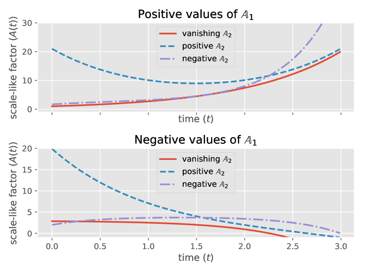
Figure 3: Behaviour of the function $A(t)$ for certain values of the parameters $(\mathbb{A}_{1},\mathbb{A}_{2},\kappa,C_{h},C_{f})$

We were able to solve the field equations for the harmonic curvature in the case $\beta_{3}=0$, which introduces interesting models of cosmologies through the appearance of the incomplete gamma function within the scale factor [see Eq. (60)]. In Fig. 4 the behaviour of the scale-like factor $A(t)$ is shown for a set of values of the parameters $(\mathbb{A}_{1},\mathbb{A}_{2},\kappa,C_{f})$. Notice the complex behaviour for the particular case with dashed lines.

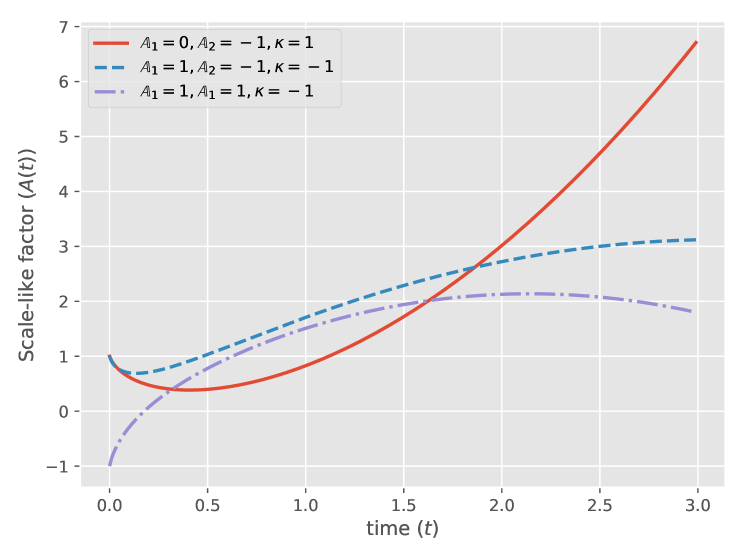
Figure 4: Behaviour of the function $A(t)$ in Eq. (60), for certain values of the parameters $(\mathbb{A}_{1},\mathbb{A}_{2},\kappa,C_{f})$

It is noticeable that connections with harmonic curvature could provide an emergent metric (i.e. Ricci tensor) corresponding to the standard metric on a Eucliean or Minkowskian space, even though their curvature do not vanish.

Further studies, which take the nature of the dark sector into account, will need to be undertaken. Interesting proposals—in models other than the Polynomial Affine model of Gravity—could be found in Ref. Josset et al. (2017); Brensinger et al. (2019); Cervantes-Cota and Liebscher (2016); Barrow et al. (2019); Kilic (2019); Roberts (1995); Chothe et al. (2019); Boskoff and Capozziello (2019).

Appendix A Building the simplified polynomial affine action

Our goal is to build the most general action using the irreducible fields, $\Gamma_{{\mu}}{}^{{\lambda}}{}_{{\nu}}$, $\mathcal{B}_{{\mu}}{}^{{\lambda}}{}_{{\nu}}$ and ${\mathcal{A}}_{\mu}$, where the dynamics is given by the covariant derivative with respect to the symmetric part of the connection, i.e., $\nabla=\nabla^{\hat{\Gamma}}$. Now, the strategy to write down the action is to define the most general scalar density. For that sake, inspired by the procedure described in Ref. Castillo-Felisola and Skirzewski (2018), we introduced a two operators, $\mathscr{N}$ and $\mathscr{W}$, that count the number of free indices and the weight density—respectively—of a given term.

The action of the operators $\mathscr{N}$and $\mathscr{W}$on the irreducible components of the connection,

$$\mathscr{N}({\mathcal{A}}) =-1, \mathscr{N}(\mathcal{B}) =-1,$$ (77)

$$\mathscr{N}(\nabla) =-1, \mathscr{N}(\mathop{\mathrm{d}V}\nolimits) =4,$$

$$\mathscr{W}({\mathcal{A}}) =0, \mathscr{W}(\mathcal{B}) =0,$$

$$\mathscr{W}(\nabla) =0, \mathscr{W}(\mathop{\mathrm{d}V}\nolimits) =1.$$

As example of how the dimensional analysis works, we consider a general term of the form $\mathcal{O}={\mathcal{A}}^{m}\mathcal{B}^{n}\nabla^{p}\mathop{\mathrm{d}V}\nolimits^{q}$, the action of the $\mathscr{N}$and $\mathscr{W}$operators on the term yield the equations

$$\mathscr{N}(\mathcal{O}) =4q-m-n-p,$$ (78)

$$\mathscr{W}(\mathcal{O}) =q.$$

We are interested in the Lagrangian, i.e. a scalar density. Equations (78) require $q=1$ and $m+n+p=4$. The terms contributing to this construction are shown in Table 1.

Table 1: Possible terms contributing to the action of Polynomial Affine Gravity

$m$	$n$	$p$	Terms
4	0	0	${\mathcal{A}}{\mathcal{A}}{\mathcal{A}}{\mathcal{A}}$
3	1	0	${\mathcal{A}}{\mathcal{A}}{\mathcal{A}}\mathcal{B}$
3	0	1	${\mathcal{A}}{\mathcal{A}}{\mathcal{A}}\nabla$
2	2	0	${\mathcal{A}}{\mathcal{A}}\mathcal{B}\mathcal{B}$
2	1	1	${\mathcal{A}}{\mathcal{A}}\mathcal{B}\nabla$
2	0	2	${\mathcal{A}}{\mathcal{A}}\nabla\nabla$
1	3	0	${\mathcal{A}}\mathcal{B}\mathcal{B}\mathcal{B}$
1	2	1	${\mathcal{A}}\mathcal{B}\mathcal{B}\nabla$
1	1	2	${\mathcal{A}}\mathcal{B}\nabla\nabla$
1	0	3	${\mathcal{A}}\nabla\nabla\nabla$
0	4	0	$\mathcal{B}\mathcal{B}\mathcal{B}\mathcal{B}$
0	3	1	$\mathcal{B}\mathcal{B}\mathcal{B}\nabla$
0	2	2	$\mathcal{B}\mathcal{B}\nabla\nabla$
0	1	3	$\mathcal{B}\nabla\nabla\nabla$
0	0	4	$\nabla\nabla\nabla\nabla$

From Table 1 one can straightforwardly read terms that vanish, e.g. the term with four ${\mathcal{A}}$ does not contribute to the action since its contraction with the volume element is identically zero. Whenever two covariant derivatives are contracted with the volume form they give a curvature tensor, and since the curvature is defined for the symmetric component of the connection, such curvature satisfy the torsion-free Bianchi identities, which relate some of the several possible contractions of indices. An additional argument that helps to drop contraction of indices is that $\mathcal{B}$ is traceless. Finally, the terms contributing to the action come from

$${\mathcal{A}}{\mathcal{A}}\mathcal{B}\mathcal{B} \rightarrow F_{4} {\mathcal{A}}{\mathcal{A}}\mathcal{B}\nabla \rightarrow D_{6},D_{7}$$

$${\mathcal{A}}\mathcal{B}\mathcal{B}\mathcal{B} \rightarrow F_{3} {\mathcal{A}}\mathcal{B}\mathcal{B}\nabla \rightarrow D_{4},D_{5}$$

$${\mathcal{A}}\mathcal{B}\nabla\nabla \rightarrow B_{3},B_{4},B_{5},E_{2} \mathcal{B}\mathcal{B}\mathcal{B}\mathcal{B} \rightarrow F_{1},F_{2}$$

$$\mathcal{B}\mathcal{B}\mathcal{B}\nabla \rightarrow D_{1},D_{2},D_{3} \mathcal{B}\mathcal{B}\nabla\nabla \rightarrow B_{1},B_{2},E_{1}$$

$$\mathcal{B}\nabla\nabla\nabla \rightarrow C_{1},C_{2}.$$

Appendix B Explicit calculation of the field equations

In order to obtain the field equations we proceed as proposed in Ref. Kijowski (1978), where an auxiliary field is introduced to ease the process. Additionally, we calculate the contribution of each term in the action to the field equations separately, since this allows us to obtain manageable expressions, and to check explicitly the possible consistent truncations of the model.

B.1 Field equations for $\Gamma_{\mu}{}^{\lambda}{}_{\nu}$

We shown in Sec. II.1.1 that the field equations for the symmetric part of the connection are

$$\nabla_{\mu}{{\Pi}_{\Gamma}{}^{\mu\nu}{}_{\lambda}{}^{\rho}}=\frac{\partial^{*}\mathscr{L}}{\partial\Gamma_{{\nu}}{}^{{\lambda}}{}_{{\rho}}}.$$

The asterisk on the right-hand side denotes the partial derivative with respect to the connection that is not contained in the curvature tensor.

Calculation of the ${{\Pi}_{\Gamma}{}^{\mu\nu}{}_{\lambda}{}^{\rho}}$

We start calculating the ${{z}_{\Gamma}{}^{\mu\nu}{}_{\lambda}{}^{\rho}}$ and then use the Eq. (8), to obtain

$$B_{1}: \Big{[}2\delta^{[\mu}_{\lambda}\mathcal{B}_{{\alpha}}{}^{{\nu]}}{}_{{\beta}}\mathcal{B}_{{\gamma}}{}^{{\rho}}{}_{{\delta}}+2\delta^{[\mu}_{\lambda}\mathcal{B}_{{\alpha}}{}^{{\rho]}}{}_{{\beta}}\mathcal{B}_{{\gamma}}{}^{{\nu}}{}_{{\delta}}\Big{]}\mathop{\mathrm{d}V}\nolimits^{\alpha\beta\gamma\delta}$$

$$B_{2}: 2\mathcal{B}_{{\gamma}}{}^{{\sigma}}{}_{{\delta}}\mathcal{B}_{{\sigma}}{}^{{(\rho}}{}_{{\lambda}}\mathop{\mathrm{d}V}\nolimits^{\nu)\mu\gamma\delta}$$

$$B_{3}: 2\delta^{[\mu}_{\lambda}\mathcal{B}_{{\beta}}{}^{{\nu]}}{}_{{\gamma}}{\mathcal{A}}_{\delta}\mathop{\mathrm{d}V}\nolimits^{\rho\beta\gamma\delta}+2\delta^{[\mu}_{\lambda}\mathcal{B}_{{\beta}}{}^{{\rho]}}{}_{{\gamma}}{\mathcal{A}}_{\delta}\mathop{\mathrm{d}V}\nolimits^{\nu\beta\gamma\delta}$$

$$B_{4}: -2\mathcal{B}_{{\gamma}}{}^{{(\rho}}{}_{{\delta}}{\mathcal{A}}_{\lambda}\mathop{\mathrm{d}V}\nolimits^{\nu)\mu\gamma\delta}$$

$$B_{5}: -2\mathcal{B}_{{\gamma}}{}^{{\sigma}}{}_{{\delta}}{\mathcal{A}}_{\sigma}\delta^{(\rho}_{\lambda}\mathop{\mathrm{d}V}\nolimits^{\nu)\mu\gamma\delta}$$

$$C_{1}: 2\nabla_{\beta}\mathcal{B}_{{\gamma}}{}^{{\rho}}{}_{{\delta}}\delta^{[\mu}_{\lambda}\mathop{\mathrm{d}V}\nolimits^{\nu]\beta\gamma\delta}+2\nabla_{\beta}\mathcal{B}_{{\gamma}}{}^{{\nu}}{}_{{\delta}}\delta^{[\mu}_{\lambda}\mathop{\mathrm{d}V}\nolimits^{\rho]\beta\gamma\delta}$$

$$C_{2}: -2\nabla_{\sigma}\mathcal{B}_{{\gamma}}{}^{{\sigma}}{}_{{\delta}}\delta^{(\rho}_{\lambda}\mathop{\mathrm{d}V}\nolimits^{\nu)\mu\gamma\delta}$$

Calculation of $\frac{\partial^{*}\mathscr{L}}{\partial\Gamma_{{\nu}}{}^{{\lambda}}{}_{{\rho}}}$

In Eq. (3), the connection appears explicitly (non in the curvature tensor) in the covariant derivative. However, the covariant derivative contains different terms depending on the field it is acting on. The two different terms in which the connection appears are

$$\nabla_{\alpha}\mathcal{B}_{{\beta}}{}^{{\gamma}}{}_{{\delta}}=\partial_{\alpha}\mathcal{B}_{{\beta}}{}^{{\gamma}}{}_{{\delta}}+\Gamma_{{\alpha}}{}^{{\lambda}}{}_{{\beta}}\mathcal{B}_{{\lambda}}{}^{{\gamma}}{}_{{\delta}}+\Gamma_{{\alpha}}{}^{{\lambda}}{}_{{\delta}}\mathcal{B}_{{\beta}}{}^{{\gamma}}{}_{{\lambda}}-\Gamma_{{\alpha}}{}^{{\gamma}}{}_{{\lambda}}\mathcal{B}_{{\beta}}{}^{{\lambda}}{}_{{\delta}}$$

and

$$\nabla_{\alpha}{\mathcal{A}}_{\beta}=\partial_{\alpha}{\mathcal{A}}_{\beta}-\Gamma_{{\alpha}}{}^{{\lambda}}{}_{{\beta}}{\mathcal{A}}_{\lambda}.$$

Now their partial derivatives with respect to the connection are

$$\frac{\partial\nabla_{\alpha}\mathcal{B}_{{\beta}}{}^{{\gamma}}{}_{{\delta}}}{\partial\Gamma_{{\nu}}{}^{{\lambda}}{}_{{\rho}}}=2\delta^{(\nu}_{\alpha}\delta^{\rho)}_{\beta}\mathcal{B}_{{\lambda}}{}^{{\gamma}}{}_{{\delta}}+2\delta^{(\nu}_{\alpha}\delta^{\rho)}_{\delta}\mathcal{B}_{{\beta}}{}^{{\gamma}}{}_{{\lambda}}-2\delta^{c}_{\lambda}\delta^{(\nu}_{\alpha}\mathcal{B}_{{\beta}}{}^{{\rho)}}{}_{{\delta}}$$

and

$$\frac{\nabla_{\alpha}{\mathcal{A}}_{\beta}}{\partial\Gamma_{{\nu}}{}^{{\lambda}}{}_{{\rho}}}=-2\delta^{(\nu}_{\alpha}\delta^{\rho)}_{\beta}{\mathcal{A}}_{\lambda}.$$

The terms coming from these derivatives are

$$C_{1}: 2\mathcal{R}_{{\mu\lambda}}{}^{{\mu}}{}_{{\alpha}}\mathcal{B}_{{\gamma}}{}^{{(\rho}}{}_{{\delta}}\mathop{\mathrm{d}V}\nolimits^{\nu)\alpha\gamma\delta}$$

$$C_{2}: 2\mathcal{R}_{{\alpha\beta}}{}^{{\sigma}}{}_{{\sigma}}\Big{[}2\mathcal{B}_{{\lambda}}{}^{{(\nu}}{}_{{\delta}}\mathop{\mathrm{d}V}\nolimits^{\rho)\alpha\beta\delta}-\delta^{(\nu}_{\lambda}\mathcal{B}_{{\gamma}}{}^{{\rho)}}{}_{{\delta}}\mathop{\mathrm{d}V}\nolimits^{\alpha\beta\gamma\delta}\Big{]}$$

$$D_{1}: 2\mathcal{B}_{{\tau}}{}^{{\sigma}}{}_{{\lambda}}\mathcal{B}_{{\sigma}}{}^{{\tau}}{}_{{\alpha}}\mathcal{B}_{{\gamma}}{}^{{(\rho}}{}_{{\delta}}\mathop{\mathrm{d}V}\nolimits^{\nu)\alpha\gamma\delta}$$

$$D_{2}: 2\mathcal{B}_{{\alpha}}{}^{{\sigma}}{}_{{\beta}}\mathcal{B}_{{\sigma}}{}^{{(\nu}}{}_{{\tau}}\Big{[}2\mathcal{B}_{{\lambda}}{}^{{\tau}}{}_{{\delta}}\mathop{\mathrm{d}V}\nolimits^{|\rho)\alpha\beta\delta}-\delta^{\tau}_{\lambda}\mathcal{B}_{{\gamma}}{}^{{|\rho)}}{}_{{\delta}}\mathop{\mathrm{d}V}\nolimits^{\alpha\beta\gamma\delta}\Big{]}$$

$$D_{3}: 2\mathcal{B}_{{\alpha}}{}^{{\sigma}}{}_{{\tau}}\mathcal{B}_{{\beta}}{}^{{(\nu}}{}_{{\gamma}}\Big{[}\delta^{\rho)}_{\sigma}\mathcal{B}_{{\lambda}}{}^{{\tau}}{}_{{\delta}}+\delta^{\rho)}_{\delta}\mathcal{B}_{{\sigma}}{}^{{\tau}}{}_{{\lambda}}-\delta^{\tau}_{\lambda}\mathcal{B}_{{\sigma}}{}^{{|\rho)}}{}_{{\delta}}\Big{]}\mathop{\mathrm{d}V}\nolimits^{\alpha\beta\gamma\delta}$$

$$D_{4}: -2\mathcal{B}_{{\alpha}}{}^{{\nu}}{}_{{\beta}}\mathcal{B}_{{\gamma}}{}^{{\rho}}{}_{{\delta}}{\mathcal{A}}_{\lambda}\mathop{\mathrm{d}V}\nolimits^{\alpha\beta\gamma\delta}$$

$$D_{5}: 2\mathcal{B}_{{\alpha}}{}^{{(\nu}}{}_{{\beta}}{\mathcal{A}}_{\sigma}\Big{[}2\mathcal{B}_{{\lambda}}{}^{{\sigma}}{}_{{\delta}}\mathop{\mathrm{d}V}\nolimits^{|\rho)\alpha\beta\delta}-\delta^{\sigma}_{\lambda}\mathcal{B}_{{\gamma}}{}^{{|\rho)}}{}_{{\delta}}\mathop{\mathrm{d}V}\nolimits^{\alpha\beta\gamma\delta}\Big{]}$$

$$D_{6}: 2\mathcal{B}_{{\alpha}}{}^{{(\nu}}{}_{{\beta}}{\mathcal{A}}_{\gamma}{\mathcal{A}}_{\lambda}\mathop{\mathrm{d}V}\nolimits^{\rho)\alpha\beta\gamma}$$

$$D_{7}: 0$$

$$E_{1}: 4\nabla_{\sigma}\mathcal{B}_{{\alpha}}{}^{{\sigma}}{}_{{\beta}}\Big{[}2\mathcal{B}_{{\lambda}}{}^{{(\rho}}{}_{{\delta}}\mathop{\mathrm{d}V}\nolimits^{\nu)\alpha\beta\delta}-\delta^{(\nu}_{\lambda}\mathcal{B}_{{\gamma}}{}^{{\rho)}}{}_{{\delta}}\mathop{\mathrm{d}V}\nolimits^{\alpha\beta\gamma\delta}\Big{]}$$

$$E_{2}: 2{\mathcal{F}}_{\alpha\beta}\Big{[}2\mathcal{B}_{{\lambda}}{}^{{(\rho}}{}_{{\delta}}\mathop{\mathrm{d}V}\nolimits^{\nu)\alpha\beta\delta}-\delta^{(\nu}_{\lambda}\mathcal{B}_{{\gamma}}{}^{{\rho)}}{}_{{\delta}}\mathop{\mathrm{d}V}\nolimits^{\alpha\beta\gamma\delta}\Big{]}$$

Notice that in the last set of contributions, the one coming from the term accompanied by the coupling $D_{7}$ yields zero. This is because the antisymmetrization of $\nabla{\mathcal{A}}$ is nothing but the field strength of the potential ${\mathcal{A}}$ (or the curvature of an Abelian 1-form). The strength does not depend on the symmetric connection.

Complete contribution

$$B_{1}: \nabla_{\mu}\left(\Big{[}2\delta^{[\mu}_{\lambda}\mathcal{B}_{{\alpha}}{}^{{\nu]}}{}_{{\beta}}\mathcal{B}_{{\gamma}}{}^{{\rho}}{}_{{\delta}}+2\delta^{[\mu}_{\lambda}\mathcal{B}_{{\alpha}}{}^{{\rho]}}{}_{{\beta}}\mathcal{B}_{{\gamma}}{}^{{\nu}}{}_{{\delta}}\Big{]}\mathop{\mathrm{d}V}\nolimits^{\alpha\beta\gamma\delta}\right)=0$$ (79)

$$B_{2}: \nabla_{\mu}\left(2\mathcal{B}_{{\gamma}}{}^{{\sigma}}{}_{{\delta}}\mathcal{B}_{{\sigma}}{}^{{(\rho}}{}_{{\lambda}}\mathop{\mathrm{d}V}\nolimits^{\nu)\mu\gamma\delta}\right)=0$$ (80)

$$B_{3}: \nabla_{\mu}\left(2\delta^{[\mu}_{\lambda}\mathcal{B}_{{\beta}}{}^{{\nu]}}{}_{{\gamma}}{\mathcal{A}}_{\delta}\mathop{\mathrm{d}V}\nolimits^{\rho\beta\gamma\delta}+2\delta^{[\mu}_{\lambda}\mathcal{B}_{{\beta}}{}^{{\rho]}}{}_{{\gamma}}{\mathcal{A}}_{\delta}\mathop{\mathrm{d}V}\nolimits^{\nu\beta\gamma\delta}\right)=0$$ (81)

$$B_{4}: \nabla_{\mu}\left(-2\mathcal{B}_{{\gamma}}{}^{{(\rho}}{}_{{\delta}}{\mathcal{A}}_{\lambda}\mathop{\mathrm{d}V}\nolimits^{\nu)\mu\gamma\delta}\right)=0$$ (82)

$$B_{5}: \nabla_{\mu}\left(-2\mathcal{B}_{{\gamma}}{}^{{\sigma}}{}_{{\delta}}{\mathcal{A}}_{\sigma}\delta^{(\rho}_{\lambda}\mathop{\mathrm{d}V}\nolimits^{\nu)\mu\gamma\delta}\right)=0$$ (83)

$$C_{1}: \nabla_{\mu}\left(2\nabla_{\beta}\mathcal{B}_{{\gamma}}{}^{{\rho}}{}_{{\delta}}\delta^{[\mu}_{\lambda}\mathop{\mathrm{d}V}\nolimits^{\nu]\beta\gamma\delta}+2\nabla_{\beta}\mathcal{B}_{{\gamma}}{}^{{\nu}}{}_{{\delta}}\delta^{[\mu}_{\lambda}\mathop{\mathrm{d}V}\nolimits^{\rho]\beta\gamma\delta}\right)=2\mathcal{R}_{{\mu\lambda}}{}^{{\mu}}{}_{{\alpha}}\mathcal{B}_{{\gamma}}{}^{{(\rho}}{}_{{\delta}}\mathop{\mathrm{d}V}\nolimits^{\nu)\alpha\gamma\delta}$$ (84)

$$C_{2}: \nabla_{\mu}\left(-2\nabla_{\sigma}\mathcal{B}_{{\gamma}}{}^{{\sigma}}{}_{{\delta}}\delta^{(\rho}_{\lambda}\mathop{\mathrm{d}V}\nolimits^{\nu)\mu\gamma\delta}\right)=2\mathcal{R}_{{\alpha\beta}}{}^{{\sigma}}{}_{{\sigma}}\Big{[}2\mathcal{B}_{{\lambda}}{}^{{(\nu}}{}_{{\delta}}\mathop{\mathrm{d}V}\nolimits^{\rho)\alpha\beta\delta}-\delta^{(\nu}_{\lambda}\mathcal{B}_{{\gamma}}{}^{{\rho)}}{}_{{\delta}}\mathop{\mathrm{d}V}\nolimits^{\alpha\beta\gamma\delta}\Big{]}$$ (85)

$$D_{1}: 2\mathcal{B}_{{\tau}}{}^{{\sigma}}{}_{{\lambda}}\mathcal{B}_{{\sigma}}{}^{{\tau}}{}_{{\alpha}}\mathcal{B}_{{\gamma}}{}^{{(\rho}}{}_{{\delta}}\mathop{\mathrm{d}V}\nolimits^{\nu)\alpha\gamma\delta}=0$$ (86)

$$D_{2}: 2\mathcal{B}_{{\alpha}}{}^{{\sigma}}{}_{{\beta}}\mathcal{B}_{{\sigma}}{}^{{(\nu}}{}_{{\tau}}\Big{[}2\mathcal{B}_{{\lambda}}{}^{{\tau}}{}_{{\delta}}\mathop{\mathrm{d}V}\nolimits^{|\rho)\alpha\beta\delta}-\delta^{\tau}_{\lambda}\mathcal{B}_{{\gamma}}{}^{{|\rho)}}{}_{{\delta}}\mathop{\mathrm{d}V}\nolimits^{\alpha\beta\gamma\delta}\Big{]}=0$$ (87)

$$D_{3}: 2\mathcal{B}_{{\alpha}}{}^{{\sigma}}{}_{{\tau}}\mathcal{B}_{{\beta}}{}^{{(\nu}}{}_{{\gamma}}\Big{[}\delta^{\rho)}_{\sigma}\mathcal{B}_{{\lambda}}{}^{{\tau}}{}_{{\delta}}+\delta^{\rho)}_{\delta}\mathcal{B}_{{\sigma}}{}^{{\tau}}{}_{{\lambda}}-\delta^{\tau}_{\lambda}\mathcal{B}_{{\sigma}}{}^{{|\rho)}}{}_{{\delta}}\Big{]}\mathop{\mathrm{d}V}\nolimits^{\alpha\beta\gamma\delta}=0$$ (88)

$$D_{4}: -2\mathcal{B}_{{\alpha}}{}^{{\nu}}{}_{{\beta}}\mathcal{B}_{{\gamma}}{}^{{\rho}}{}_{{\delta}}{\mathcal{A}}_{\lambda}\mathop{\mathrm{d}V}\nolimits^{\alpha\beta\gamma\delta}=0$$ (89)

$$D_{5}: 2\mathcal{B}_{{\alpha}}{}^{{(\nu}}{}_{{\beta}}{\mathcal{A}}_{\sigma}\Big{[}2\mathcal{B}_{{\lambda}}{}^{{\sigma}}{}_{{\delta}}\mathop{\mathrm{d}V}\nolimits^{|\rho)\alpha\beta\delta}-\delta^{\sigma}_{\lambda}\mathcal{B}_{{\gamma}}{}^{{|\rho)}}{}_{{\delta}}\mathop{\mathrm{d}V}\nolimits^{\alpha\beta\gamma\delta}\Big{]}=0$$ (90)

$$D_{6}: 2\mathcal{B}_{{\alpha}}{}^{{(\nu}}{}_{{\beta}}{\mathcal{A}}_{\gamma}{\mathcal{A}}_{\lambda}\mathop{\mathrm{d}V}\nolimits^{\rho)\alpha\beta\gamma}=0$$ (91)

$$E_{1}: 4\nabla_{\sigma}\mathcal{B}_{{\alpha}}{}^{{\sigma}}{}_{{\beta}}\Big{[}2\mathcal{B}_{{\lambda}}{}^{{(\rho}}{}_{{\delta}}\mathop{\mathrm{d}V}\nolimits^{\nu)\alpha\beta\delta}-\delta^{(\nu}_{\lambda}\mathcal{B}_{{\gamma}}{}^{{\rho)}}{}_{{\delta}}\mathop{\mathrm{d}V}\nolimits^{\alpha\beta\gamma\delta}\Big{]}=0$$ (92)

$$E_{2}: 2{\mathcal{F}}_{\alpha\beta}\Big{[}2\mathcal{B}_{{\lambda}}{}^{{(\rho}}{}_{{\delta}}\mathop{\mathrm{d}V}\nolimits^{\nu)\alpha\beta\delta}-\delta^{(\nu}_{\lambda}\mathcal{B}_{{\gamma}}{}^{{\rho)}}{}_{{\delta}}\mathop{\mathrm{d}V}\nolimits^{\alpha\beta\gamma\delta}\Big{]}=0$$ (93)

B.2 Field equations for $B_{\mu}{}^{\lambda}{}_{\nu}$

In Sec. II.1.2 we show that the field equations for the $\mathcal{B}$ field are

$$\nabla_{\mu}{{\Pi}_{\mathcal{B}}{}^{\mu\nu}{}_{\lambda}{}^{\rho}}=\frac{\partial\mathscr{L}}{\partial\mathcal{B}_{{\nu}}{}^{{\lambda}}{}_{{\rho}}}.$$

We now calculate explicitly the contribution of each term in the action to the above field equation.

Calculation of ${{\Pi}_{\mathcal{B}}{}^{\mu\nu}{}_{\lambda}{}^{\rho}}$

The explicit calculation of ${{\Pi}_{\mathcal{B}}{}^{\mu\nu}{}_{\lambda}{}^{\rho}}$ yield

$$C_{1}: -2\mathcal{R}_{{\sigma\alpha}}{}^{{\sigma}}{}_{{\lambda}}\mathop{\mathrm{d}V}\nolimits^{\mu\nu\rho\alpha}$$

$$C_{2}: 2\mathcal{R}_{{\alpha\beta}}{}^{{\sigma}}{}_{{\sigma}}\delta^{\mu}_{\lambda}\mathop{\mathrm{d}V}\nolimits^{\nu\rho\alpha\beta}$$

$$D_{1}: -2\mathcal{B}_{{\sigma}}{}^{{\theta}}{}_{{\lambda}}\mathcal{B}_{{\theta}}{}^{{\sigma}}{}_{{\alpha}}\mathop{\mathrm{d}V}\nolimits^{\mu\nu\rho\alpha}$$

$$D_{2}: 2\mathcal{B}_{{\alpha}}{}^{{\sigma}}{}_{{\beta}}\mathcal{B}_{{\sigma}}{}^{{\mu}}{}_{{\lambda}}\mathop{\mathrm{d}V}\nolimits^{\nu\rho\alpha\beta}$$

$$D_{3}: -2\mathcal{B}_{{\alpha}}{}^{{\nu}}{}_{{\lambda}}\mathcal{B}_{{\beta}}{}^{{\mu}}{}_{{\gamma}}\mathop{\mathrm{d}V}\nolimits^{\rho\alpha\beta\gamma}$$

$$D_{5}: 2\mathcal{B}_{{\alpha}}{}^{{\mu}}{}_{{\beta}}{\mathcal{A}}_{\lambda}\mathop{\mathrm{d}V}\nolimits^{\nu\rho\alpha\beta}$$

$$E_{1}: 4\delta^{\mu}_{\lambda}\nabla_{\sigma}\mathcal{B}_{{\alpha}}{}^{{\sigma}}{}_{{\beta}}\mathop{\mathrm{d}V}\nolimits^{\nu\rho\alpha\beta}$$

$$E_{2}: 2\delta^{\mu}_{\lambda}{\mathcal{F}}_{\alpha\beta}\mathop{\mathrm{d}V}\nolimits^{\nu\rho\alpha\beta}$$

Calculation of $\frac{\partial\mathscr{L}}{\partial\mathcal{B}_{{\nu}}{}^{{\lambda}}{}_{{\rho}}}$

The contributions to the right-hand side of the field equations for the $\mathcal{B}$-field are,

$$B_{1}: 4\mathcal{R}_{{\mu(\sigma}}{}^{{\mu}}{}_{{\lambda)}}\mathcal{B}_{{\gamma}}{}^{{\sigma}}{}_{{\delta}}\mathop{\mathrm{d}V}\nolimits^{\nu\rho\gamma\delta}$$

$$B_{2}: 2\mathcal{R}_{{\alpha\beta}}{}^{{\mu}}{}_{{\sigma}}\mathcal{B}_{{\mu}}{}^{{\sigma}}{}_{{\lambda}}\mathop{\mathrm{d}V}\nolimits^{\nu\rho\alpha\beta}+2\mathcal{R}_{{\alpha\beta}}{}^{{[\nu}}{}_{{\lambda}}\mathcal{B}_{{\gamma}}{}^{{\rho]}}{}_{{\delta}}\mathop{\mathrm{d}V}\nolimits^{\alpha\beta\gamma\delta}$$

$$B_{3}: 2\mathcal{R}_{{\mu\lambda}}{}^{{\mu}}{}_{{\alpha}}{\mathcal{A}}_{\beta}\mathop{\mathrm{d}V}\nolimits^{\nu\rho\alpha\beta}$$

$$B_{4}: 2\mathcal{R}_{{\alpha\beta}}{}^{{\sigma}}{}_{{\lambda}}{\mathcal{A}}_{\sigma}\mathop{\mathrm{d}V}\nolimits^{\nu\rho\alpha\beta}$$

$$B_{5}: 2\mathcal{R}_{{\alpha\beta}}{}^{{\tau}}{}_{{\tau}}{\mathcal{A}}_{\lambda}\mathop{\mathrm{d}V}\nolimits^{\nu\rho\alpha\beta}$$

$$D_{1}: 2\mathcal{B}_{{\lambda}}{}^{{[\nu}}{}_{{\alpha}}\nabla_{\beta}\mathcal{B}_{{\gamma}}{}^{{\rho]}}{}_{{\delta}}\mathop{\mathrm{d}V}\nolimits^{\alpha\beta\gamma\delta}+2\mathcal{B}_{{\lambda}}{}^{{[\nu|}}{}_{{\sigma}}\nabla_{\beta}\mathcal{B}_{{\gamma}}{}^{{\sigma}}{}_{{\delta}}\mathop{\mathrm{d}V}\nolimits^{|\rho]\beta\gamma\delta}$$

$$D_{2}: 2\mathcal{B}_{{\lambda}}{}^{{\mu}}{}_{{\sigma}}\nabla_{\mu}\mathcal{B}_{{\alpha}}{}^{{\sigma}}{}_{{\beta}}\mathop{\mathrm{d}V}\nolimits^{\nu\rho\alpha\beta}+2\mathcal{B}_{{\alpha}}{}^{{[\nu}}{}_{{\beta}}\nabla_{\lambda}\mathcal{B}_{{\gamma}}{}^{{\rho]}}{}_{{\delta}}\mathop{\mathrm{d}V}\nolimits^{\alpha\beta\gamma\delta}$$

$$D_{3}: 2\mathcal{B}_{{\beta}}{}^{{\mu}}{}_{{\gamma}}\nabla_{\mu}\mathcal{B}_{{\lambda}}{}^{{[\rho}}{}_{{\delta}}\mathop{\mathrm{d}V}\nolimits^{\nu]\beta\gamma\delta}+2\mathcal{B}_{{\gamma}}{}^{{\mu}}{}_{{\sigma}}\nabla_{\lambda}\mathcal{B}_{{\mu}}{}^{{\sigma}}{}_{{\delta}}\mathop{\mathrm{d}V}\nolimits^{\nu\rho\gamma\delta}$$

$$D_{4}: 4\mathcal{B}_{{\alpha}}{}^{{\sigma}}{}_{{\beta}}\nabla_{(\lambda}{\mathcal{A}}_{\sigma)}\mathop{\mathrm{d}V}\nolimits^{\nu\rho\alpha\beta}$$

$$D_{5}: 2\nabla_{\lambda}\mathcal{B}_{{\alpha}}{}^{{\sigma}}{}_{{\beta}}{\mathcal{A}}_{\sigma}\mathop{\mathrm{d}V}\nolimits^{\nu\rho\alpha\beta}$$

$$D_{6}: 2{\mathcal{A}}_{\gamma}\nabla_{\lambda}{\mathcal{A}}_{\delta}\mathop{\mathrm{d}V}\nolimits^{\nu\rho\gamma\delta}$$

$$D_{7}: 2{\mathcal{A}}_{\lambda}F_{\gamma\delta}\mathop{\mathrm{d}V}\nolimits^{\nu\rho\gamma\delta}$$

$$F_{1}: 4\mathcal{B}_{{\alpha}}{}^{{\mu}}{}_{{\beta}}\mathcal{B}_{{\mu}}{}^{{\sigma}}{}_{{\tau}}\mathcal{B}_{{\lambda}}{}^{{\tau}}{}_{{\sigma}}\mathop{\mathrm{d}V}\nolimits^{\nu\rho\alpha\beta}+4\mathcal{B}_{{\alpha}}{}^{{\mu}}{}_{{\beta}}\mathcal{B}_{{\gamma}}{}^{{[\nu}}{}_{{\delta}}\mathcal{B}_{{\mu}}{}^{{\rho]}}{}_{{\lambda}}\mathop{\mathrm{d}V}\nolimits^{\alpha\beta\gamma\delta}$$

$$F_{2}: 2\mathcal{B}_{{\alpha}}{}^{{\mu}}{}_{{\sigma}}\mathcal{B}_{{\beta}}{}^{{\sigma}}{}_{{\tau}}\mathcal{B}_{{\lambda}}{}^{{\tau}}{}_{{\mu}}\mathop{\mathrm{d}V}\nolimits^{\nu\rho\alpha\beta}+2\mathcal{B}_{{\alpha}}{}^{{\mu}}{}_{{\beta}}\mathcal{B}_{{\mu}}{}^{{\sigma}}{}_{{\lambda}}\mathcal{B}_{{\gamma}}{}^{{[\rho}}{}_{{\sigma}}\mathop{\mathrm{d}V}\nolimits^{\nu]\alpha\beta\gamma}$$

$$-2\mathcal{B}_{{\alpha}}{}^{{\mu}}{}_{{\beta}}\mathcal{B}_{{\gamma}}{}^{{\sigma}}{}_{{\lambda}}\mathcal{B}_{{\mu}}{}^{{[\rho}}{}_{{\sigma}}\mathop{\mathrm{d}V}\nolimits^{\nu]\alpha\beta\gamma}+2\mathcal{B}_{{\alpha}}{}^{{[\nu}}{}_{{\beta}}\mathcal{B}_{{\gamma}}{}^{{\rho]}}{}_{{\sigma}}\mathcal{B}_{{\delta}}{}^{{\sigma}}{}_{{\lambda}}\mathop{\mathrm{d}V}\nolimits^{\alpha\beta\gamma\delta}$$

$$F_{3}: 2\mathcal{B}_{{\lambda}}{}^{{[\nu}}{}_{{\alpha}}\mathcal{B}_{{\beta}}{}^{{\rho]}}{}_{{\gamma}}{\mathcal{A}}_{\delta}\mathop{\mathrm{d}V}\nolimits^{\alpha\beta\gamma\delta}+2\mathcal{B}_{{\alpha}}{}^{{\sigma}}{}_{{\beta}}{\mathcal{A}}_{\gamma}\mathcal{B}_{{\lambda}}{}^{{[\nu}}{}_{{\sigma}}\mathop{\mathrm{d}V}\nolimits^{\rho]\alpha\beta\gamma}$$

$$\quad+2\mathcal{B}_{{\sigma}}{}^{{\mu}}{}_{{\lambda}}\mathcal{B}_{{\mu}}{}^{{\sigma}}{}_{{\alpha}}{\mathcal{A}}_{\beta}\mathop{\mathrm{d}V}\nolimits^{\nu\rho\alpha\beta}$$

$$F_{4}: 4\mathcal{B}_{{\alpha}}{}^{{\mu}}{}_{{\beta}}{\mathcal{A}}_{\mu}{\mathcal{A}}_{\lambda}\mathop{\mathrm{d}V}\nolimits^{\nu\rho\alpha\beta}$$

Complete contribution

$$B_{1}: 4\mathcal{R}_{{\mu(\sigma}}{}^{{\mu}}{}_{{\lambda)}}\mathcal{B}_{{\gamma}}{}^{{\sigma}}{}_{{\delta}}\mathop{\mathrm{d}V}\nolimits^{\nu\rho\gamma\delta}=0$$ (94)

$$B_{2}: 2\mathcal{R}_{{\alpha\beta}}{}^{{\mu}}{}_{{\sigma}}\mathcal{B}_{{\mu}}{}^{{\sigma}}{}_{{\lambda}}\mathop{\mathrm{d}V}\nolimits^{\nu\rho\alpha\beta}+2\mathcal{R}_{{\alpha\beta}}{}^{{[\nu}}{}_{{\lambda}}\mathcal{B}_{{\gamma}}{}^{{\rho]}}{}_{{\delta}}\mathop{\mathrm{d}V}\nolimits^{\alpha\beta\gamma\delta}=0$$ (95)

$$B_{3}: 2\mathcal{R}_{{\mu\lambda}}{}^{{\mu}}{}_{{\alpha}}{\mathcal{A}}_{\beta}\mathop{\mathrm{d}V}\nolimits^{\nu\rho\alpha\beta}=0$$ (96)

$$B_{4}: 2\mathcal{R}_{{\alpha\beta}}{}^{{\sigma}}{}_{{\lambda}}{\mathcal{A}}_{\sigma}\mathop{\mathrm{d}V}\nolimits^{\nu\rho\alpha\beta}=0$$ (97)

$$B_{5}: 2\mathcal{R}_{{\alpha\beta}}{}^{{\tau}}{}_{{\tau}}{\mathcal{A}}_{\lambda}\mathop{\mathrm{d}V}\nolimits^{\nu\rho\alpha\beta}=0$$ (98)

$$C_{1}: \nabla_{\mu}\left(-2\mathcal{R}_{{\sigma\alpha}}{}^{{\sigma}}{}_{{\lambda}}\mathop{\mathrm{d}V}\nolimits^{\mu\nu\rho\alpha}\right)=0$$ (99)

$$C_{2}: \nabla_{\mu}\left(2\mathcal{R}_{{\alpha\beta}}{}^{{\sigma}}{}_{{\sigma}}\delta^{\mu}_{\lambda}\mathop{\mathrm{d}V}\nolimits^{\nu\rho\alpha\beta}\right)=0$$ (100)

$$D_{1}: \nabla_{\mu}\left(-2\mathcal{B}_{{\sigma}}{}^{{\theta}}{}_{{\lambda}}\mathcal{B}_{{\theta}}{}^{{\sigma}}{}_{{\alpha}}\mathop{\mathrm{d}V}\nolimits^{\mu\nu\rho\alpha}\right)=2\mathcal{B}_{{\lambda}}{}^{{[\nu}}{}_{{\alpha}}\nabla_{\beta}\mathcal{B}_{{\gamma}}{}^{{\rho]}}{}_{{\delta}}\mathop{\mathrm{d}V}\nolimits^{\alpha\beta\gamma\delta}+2\mathcal{B}_{{\lambda}}{}^{{[\nu|}}{}_{{\sigma}}\nabla_{\beta}\mathcal{B}_{{\gamma}}{}^{{\sigma}}{}_{{\delta}}\mathop{\mathrm{d}V}\nolimits^{|\rho]\beta\gamma\delta}$$ (101)

$$D_{2}: \nabla_{\mu}\left(2\mathcal{B}_{{\alpha}}{}^{{\sigma}}{}_{{\beta}}\mathcal{B}_{{\sigma}}{}^{{\mu}}{}_{{\lambda}}\mathop{\mathrm{d}V}\nolimits^{\nu\rho\alpha\beta}\right)=2\mathcal{B}_{{\lambda}}{}^{{\mu}}{}_{{\sigma}}\nabla_{\mu}\mathcal{B}_{{\alpha}}{}^{{\sigma}}{}_{{\beta}}\mathop{\mathrm{d}V}\nolimits^{\nu\rho\alpha\beta}+2\mathcal{B}_{{\alpha}}{}^{{[\nu}}{}_{{\beta}}\nabla_{\lambda}\mathcal{B}_{{\gamma}}{}^{{\rho]}}{}_{{\delta}}\mathop{\mathrm{d}V}\nolimits^{\alpha\beta\gamma\delta}$$ (102)

$$D_{3}: \nabla_{\mu}\left(-2\mathcal{B}_{{\alpha}}{}^{{\nu}}{}_{{\lambda}}\mathcal{B}_{{\beta}}{}^{{\mu}}{}_{{\gamma}}\mathop{\mathrm{d}V}\nolimits^{\rho\alpha\beta\gamma}\right)=2\mathcal{B}_{{\beta}}{}^{{\mu}}{}_{{\gamma}}\nabla_{\mu}\mathcal{B}_{{\lambda}}{}^{{[\rho}}{}_{{\delta}}\mathop{\mathrm{d}V}\nolimits^{\nu]\beta\gamma\delta}+2\mathcal{B}_{{\gamma}}{}^{{\mu}}{}_{{\sigma}}\nabla_{\lambda}\mathcal{B}_{{\mu}}{}^{{\sigma}}{}_{{\delta}}\mathop{\mathrm{d}V}\nolimits^{\nu\rho\gamma\delta}$$ (103)

$$D_{4}: 4\mathcal{B}_{{\alpha}}{}^{{\sigma}}{}_{{\beta}}\nabla_{(\lambda}{\mathcal{A}}_{\sigma)}\mathop{\mathrm{d}V}\nolimits^{\nu\rho\alpha\beta}=0$$ (104)

$$D_{5}: \nabla_{\mu}\left(2\mathcal{B}_{{\alpha}}{}^{{\mu}}{}_{{\beta}}{\mathcal{A}}_{\lambda}\mathop{\mathrm{d}V}\nolimits^{\nu\rho\alpha\beta}\right)=2\nabla_{\lambda}\mathcal{B}_{{\alpha}}{}^{{\sigma}}{}_{{\beta}}{\mathcal{A}}_{\sigma}\mathop{\mathrm{d}V}\nolimits^{\nu\rho\alpha\beta}$$ (105)

$$D_{6}: 2{\mathcal{A}}_{\gamma}\nabla_{\lambda}{\mathcal{A}}_{\delta}\mathop{\mathrm{d}V}\nolimits^{\nu\rho\gamma\delta}=0$$ (106)

$$D_{7}: 2{\mathcal{A}}_{\lambda}F_{\gamma\delta}\mathop{\mathrm{d}V}\nolimits^{\nu\rho\gamma\delta}=0$$ (107)

$$E_{1}: \nabla_{\mu}\left(4\delta^{\mu}_{\lambda}\nabla_{\sigma}\mathcal{B}_{{\alpha}}{}^{{\sigma}}{}_{{\beta}}\mathop{\mathrm{d}V}\nolimits^{\nu\rho\alpha\beta}\right)=0$$ (108)

$$E_{2}: \nabla_{\mu}\left(2\delta^{\mu}_{\lambda}{\mathcal{F}}_{\alpha\beta}\mathop{\mathrm{d}V}\nolimits^{\nu\rho\alpha\beta}\right)=0$$ (109)

$$F_{1}: 4\mathcal{B}_{{\alpha}}{}^{{\mu}}{}_{{\beta}}\mathcal{B}_{{\mu}}{}^{{\sigma}}{}_{{\tau}}\mathcal{B}_{{\lambda}}{}^{{\tau}}{}_{{\sigma}}\mathop{\mathrm{d}V}\nolimits^{\nu\rho\alpha\beta}+4\mathcal{B}_{{\alpha}}{}^{{\mu}}{}_{{\beta}}\mathcal{B}_{{\gamma}}{}^{{[\nu}}{}_{{\delta}}\mathcal{B}_{{\mu}}{}^{{\rho]}}{}_{{\lambda}}\mathop{\mathrm{d}V}\nolimits^{\alpha\beta\gamma\delta}=0$$ (110)

$$F_{2}: 2\mathcal{B}_{{\alpha}}{}^{{\mu}}{}_{{\sigma}}\mathcal{B}_{{\beta}}{}^{{\sigma}}{}_{{\tau}}\mathcal{B}_{{\lambda}}{}^{{\tau}}{}_{{\mu}}\mathop{\mathrm{d}V}\nolimits^{\nu\rho\alpha\beta}+2\mathcal{B}_{{\alpha}}{}^{{\mu}}{}_{{\beta}}\mathcal{B}_{{\mu}}{}^{{\sigma}}{}_{{\lambda}}\mathcal{B}_{{\gamma}}{}^{{[\rho}}{}_{{\sigma}}\mathop{\mathrm{d}V}\nolimits^{\nu]\alpha\beta\gamma}$$

$$-2\mathcal{B}_{{\alpha}}{}^{{\mu}}{}_{{\beta}}\mathcal{B}_{{\gamma}}{}^{{\sigma}}{}_{{\lambda}}\mathcal{B}_{{\mu}}{}^{{[\rho}}{}_{{\sigma}}\mathop{\mathrm{d}V}\nolimits^{\nu]\alpha\beta\gamma}+2\mathcal{B}_{{\alpha}}{}^{{[\nu}}{}_{{\beta}}\mathcal{B}_{{\gamma}}{}^{{\rho]}}{}_{{\sigma}}\mathcal{B}_{{\delta}}{}^{{\sigma}}{}_{{\lambda}}\mathop{\mathrm{d}V}\nolimits^{\alpha\beta\gamma\delta}=0$$ (111)

$$F_{3}: 2\mathcal{B}_{{\lambda}}{}^{{[\nu}}{}_{{\alpha}}\mathcal{B}_{{\beta}}{}^{{\rho]}}{}_{{\gamma}}{\mathcal{A}}_{\delta}\mathop{\mathrm{d}V}\nolimits^{\alpha\beta\gamma\delta}+2\mathcal{B}_{{\alpha}}{}^{{\sigma}}{}_{{\beta}}{\mathcal{A}}_{\gamma}\mathcal{B}_{{\lambda}}{}^{{[\nu}}{}_{{\sigma}}\mathop{\mathrm{d}V}\nolimits^{\rho]\alpha\beta\gamma}+2\mathcal{B}_{{\sigma}}{}^{{\mu}}{}_{{\lambda}}\mathcal{B}_{{\mu}}{}^{{\sigma}}{}_{{\alpha}}{\mathcal{A}}_{\beta}\mathop{\mathrm{d}V}\nolimits^{\nu\rho\alpha\beta}=0$$ (112)

$$F_{4}: 4\mathcal{B}_{{\alpha}}{}^{{\mu}}{}_{{\beta}}{\mathcal{A}}_{\mu}{\mathcal{A}}_{\lambda}\mathop{\mathrm{d}V}\nolimits^{\nu\rho\alpha\beta}=0$$ (113)

B.3 Field equations for ${\mathcal{A}}_{\mu}$

In this section, we show the complete Euler–Lagrage equations for the ${\mathcal{A}}$ field.

$$B_{3}: \mathcal{R}_{{\sigma\tau}}{}^{{\sigma}}{}_{{\alpha}}\mathcal{B}_{{\beta}}{}^{{\tau}}{}_{{\gamma}}\mathop{\mathrm{d}V}\nolimits^{\alpha\beta\gamma\nu}=0$$ (114)

$$B_{4}: \mathcal{R}_{{\alpha\beta}}{}^{{\nu}}{}_{{\sigma}}\mathcal{B}_{{\gamma}}{}^{{\sigma}}{}_{{\delta}}\mathop{\mathrm{d}V}\nolimits^{\alpha\beta\gamma\delta}=0$$ (115)

$$B_{5}: \mathcal{R}_{{\alpha\beta}}{}^{{\sigma}}{}_{{\sigma}}\mathcal{B}_{{\gamma}}{}^{{\nu}}{}_{{\delta}}\mathop{\mathrm{d}V}\nolimits^{\alpha\beta\gamma\delta}=0$$ (116)

$$D_{4} \nabla_{\mu}\Big{[}\mathcal{B}_{{\alpha}}{}^{{\mu}}{}_{{\beta}}\mathcal{B}_{{\gamma}}{}^{{\nu}}{}_{{\delta}}\mathop{\mathrm{d}V}\nolimits^{\alpha\beta\gamma\delta}\Big{]}=0$$ (117)

$$D_{5}: \mathcal{B}_{{\alpha}}{}^{{\sigma}}{}_{{\beta}}\nabla_{\sigma}\mathcal{B}_{{\gamma}}{}^{{\nu}}{}_{{\delta}}\mathop{\mathrm{d}V}\nolimits^{\alpha\beta\gamma\delta}=0$$ (118)

$$D_{6}: \nabla_{\mu}\Big{[}\mathcal{B}_{{\alpha}}{}^{{\mu}}{}_{{\beta}}{\mathcal{A}}_{\gamma}\mathop{\mathrm{d}V}\nolimits^{\alpha\beta\gamma\nu}\Big{]}+\mathcal{B}_{{\alpha}}{}^{{\mu}}{}_{{\beta}}\nabla_{\mu}{\mathcal{A}}_{\gamma}\mathop{\mathrm{d}V}\nolimits^{\alpha\beta\gamma\nu}=0$$ (119)

$$D_{7}: \nabla_{\mu}\Big{[}\mathcal{B}_{{\alpha}}{}^{{\sigma}}{}_{{\beta}}{\mathcal{A}}_{\sigma}\mathop{\mathrm{d}V}\nolimits^{\alpha\beta\mu\nu}\Big{]}+\mathcal{B}_{{\alpha}}{}^{{\nu}}{}_{{\beta}}{\mathcal{F}}_{\gamma\delta}\mathop{\mathrm{d}V}\nolimits^{\alpha\beta\gamma\delta}=0$$ (120)

$$E_{2}: \nabla_{\mu}\Big{[}\nabla_{\sigma}\mathcal{B}_{{\alpha}}{}^{{\sigma}}{}_{{\beta}}\mathop{\mathrm{d}V}\nolimits^{\alpha\beta\mu\nu}\Big{]}=0$$ (121)

$$F_{3}: \mathcal{B}_{{\sigma}}{}^{{\tau}}{}_{{\lambda}}\mathcal{B}_{{\tau}}{}^{{\sigma}}{}_{{\alpha}}\mathcal{B}_{{\beta}}{}^{{\lambda}}{}_{{\gamma}}\mathop{\mathrm{d}V}\nolimits^{\alpha\beta\gamma\nu}=0$$ (122)

$$F_{4}: 2\mathcal{B}_{{\alpha}}{}^{{\sigma}}{}_{{\beta}}\mathcal{B}_{{\gamma}}{}^{{\nu}}{}_{{\delta}}{\mathcal{A}}_{\sigma}\mathop{\mathrm{d}V}\nolimits^{\alpha\beta\gamma\delta}=0$$ (123)

References

- Einstein (1915a) Albert Einstein, “Grundgedanken der allgemeinen relativitätstheorie und anwendung dieser theorie in der astronomie,” Preussische Akademie der Wissenschaften, Sitzungsberichte 315, 778–786 (1915a).
- Einstein (1915b) Albert Einstein, “Zur allgemeinen relativitätstheorie,” Sitzungsber. preuss. Akad. Wiss. 1, 778 (1915b).
- Einstein (1915c) Albert Einstein, “Erklarung der perihelionbewegung der merkur aus der allgemeinen relativitatstheorie,” Sitzungsber. preuss. Akad. Wiss. 47, 831 (1915c).
- Einstein (1915d) Albert Einstein, “Die feldgleichungen der gravitation,” Sitzungsber. preuss. Akad. Wiss. 1, 844 (1915d).
- Einstein (1916) Albert Einstein, “Die grundlage der allgemeinen relativitätstheorie,” Ann. Phys. 49, 284–339 (1916).
- Will (2014) Clifford M. Will, “The Confrontation Between Gerenal Relativity and experiment,” Living Rev. Rel. 17, 4 (2014), arXiv:1403.7377 [gr-qc] .
- Abbott et al. (2016) B. P. Abbott et al. (Virgo, LIGO Scientific), “GW151226: Observation of Gravitational Waves From a 22-solar-Mass Binary Black Hole Coalescence,” Phys. Rev. Lett. 116, 241103 (2016), arXiv:1606.04855 [gr-qc] .
- Abbott et al. (2017) B. P. Abbott et al., “Gravitational waves and gamma-rays from a binary neutron star merger: Gw170817 and grb170817a,” Astrophys. J. 848, L13 (2017).
- DeWitt (1967a) Bryce S. DeWitt, “Quantum Theory of Gravity. 1. The Canonical Theory,” Phys. Rev. 160, 1113 (1967a).
- DeWitt (1967b) Bryce S. DeWitt, “Quantum Theory of Gravity. 2. The Manifestly Covariant Theory,” Phys. Rev. 162, 1195 (1967b).
- Deser and van Nieuwenhuizen (1974a) Stanley Deser and P. van Nieuwenhuizen, “One Loop Divergences of Quantized Einstein-Maxwell Fields,” Phys. Rev. D 10, 401 (1974a).
- Deser and van Nieuwenhuizen (1974b) Stanley Deser and P. van Nieuwenhuizen, “Nonrenormalizability of the Quantized Dirac-Einstein System,” Phys. Rev. D 10, 411 (1974b).
- ’t Hooft and Veltman (1974) Gerard ’t Hooft and M. J. G. Veltman, “One Loop Divergencies in the Theory of gravitation,” Annales Poincare Phys. Theor. A 20, 69 (1974).
- Ashtekar (1986) A. Ashtekar, “New Variables for Classical and Quantum Gravity,” Phys. Rev. Lett. 57, 2244–2247 (1986).
- Ashtekar (1987) A. Ashtekar, “New Hamiltonian Formulation of General Relativity,” Phys. Rev. D 36, 1587 (1987).
- Zwicky (1937) F. Zwicky, “On the masses of nebulae and of clusters of nebulae,” Astrophys. J. 86, 217 (1937).
- Rubin and W. Kent (1970) Vera C. Rubin and Jr. W. Kent, Ford, “Rotation of the andromeda nebula from a spectroscopic survey of emission regions,” Astrophys. J. 159, 379 (1970).
- Sofue and Rubin (2001) Yoshiaki Sofue and Vera Rubin, “Rotation Curves of Spiral galaxies,” Ann. Rev. Astron. Astrophys. 39, 137 (2001), arXiv:astro-ph/0010594 [astro-ph] .
- Riess et al. (1998) Adam G. Riess et al. (Supernova Search Team), “Observational Evidence From Supernovae for an Accelerating Universe and a Cosmological constant,” Astron. J. 116, 1009 (1998), arXiv:astro-ph/9805201 [astro-ph] .
- Perlmutter et al. (1999) S. Perlmutter et al. (Supernova Cosmology Project), “Measurements of and From 42 High-Redshift Supernovae,” Astrophys. J. 517, 565 (1999).
- Cartan (1922) Elie Cartan, “Sur une généralisation de la notion de courbure de riemann et les espaces à torsion,” C. R. Acad. Sci. Paris 174, 593 (1922).
- Cartan (1923) Elie Cartan, “Sur les variétés à connexion affine et la théorie de la relativité généralisée (première partie),” Ann. Ec. Norm. Super. 40, 325 (1923).
- Cartan (1924) Elie Cartan, “Sur les variétés à connexion affine, et la théorie de la relativité généralisée (première partie) (suite),” Ann. Ec. Norm. Super. 41, 1 (1924).
- Cartan (1925) Elie Cartan, “Sur les variétés à connexion affine et la théorie de la relativité généralisée, (deuxième partie),” Ann. Ec. Norm. Super. 42, 17 (1925).
- Kaluza (1921) Theodor Kaluza, “On the Problem of Unity in Physics,” Sitzungsber. Preuss. Akad. Wiss. Berlin (Math. Phys.) 1921, 966 (1921).
- Klein (1926) O. Klein, “Quantum Theory and Five-Dimensional Theory of relativity,” Z. Phys. 37, 895 (1926).
- Lovelock (1971) David Lovelock, “The Einstein Tensor and Its generalizations,” J. Math. Phys. 12, 498–501 (1971).
- Hehl et al. (1995) Friedrich W. Hehl, J. Dermott McCrea, Eckehard W. Mielke, and Yuval Ne’eman, “Metric Affine Gauge Theory of Gravity: Field Equations, Noether Identities, World Spinors, and Breaking of Dilation invariance,” Phys. Rep. 258, 1–171 (1995), arXiv:gr-qc/9402012 [gr-qc] .
- Mardones and Zanelli (1991) Alejandro Mardones and Jorge Zanelli, “Lovelock–Cartan Theory of gravity,” Class. Quant. Grav. 8, 1545 (1991).
- Eddington (1923) Arthur S. Eddington, The mathematical theory of relativity (Cambridge University Press, 1923).
- Schrödinger (1950) Erwin Schrödinger, Space-time structure (Cambridge University Press, 1950).
- Kijowski (1978) Jerzy Kijowski, “On a new variational principle in general relativity and the energy of the gravitational field,” Gen. Rel. Grav. 9, 857 (1978).
- Krasnov (2006) Kirill Krasnov, “Renormalizable Non-Metric Quantum Gravity?” (2006), arXiv:hep-th/0611182 [hep-th] .
- Krasnov (2007) Kirill Krasnov, “Non-Metric Gravity: A Status report,” Mod. Phys. Lett. A 22, 3013–3026 (2007), arXiv:0711.0697 [gr-qc] .
- Krasnov (2008) Kirill Krasnov, “Non-Metric Gravity. I. Field Equations,” Class. Quant. Grav. 25, 025001 (2008), arXiv:gr-qc/0703002 [gr-qc] .
- Krasnov and Shtanov (2008) Kirill Krasnov and Yuri Shtanov, “Non-Metric Gravity. II. Spherically Symmetric Solution, Missing Mass and Redshifts of Quasars,” Class. Quant. Grav. 25, 025002 (2008), arXiv:0705.2047 [gr-qc] .
- Krasnov (2011) Kirill Krasnov, “Pure Connection Action Principle for General Relativity,” Phys. Rev. Lett. 106, 251103 (2011), arXiv:1103.4498 [gr-qc] .
- Popławski (2007a) Nikodem J. Popławski, “A unified, purely affine theory of gravitation and electromagnetism,” (2007a), arXiv:0705.0351 [gr-qc] .
- Popławski (2007b) Nikodem J. Popławski, “On the Nonsymmetric Purely Affine gravity,” Mod. Phys. Lett. A 22, 2701 (2007b), arXiv:gr-qc/0610132 [gr-qc] .
- Popławski (2014) Nikodem J. Popławski, “Affine Theory of gravitation,” Gen. Rel. Grav. 46, 1625 (2014), arXiv:1203.0294 [gr-qc] .
- Castillo-Felisola and Skirzewski (2015) Oscar Castillo-Felisola and Aureliano Skirzewski, “A Polynomial Model of Purely Affine Gravity,” Rev. Mex. Fis. 61, 421 (2015), arXiv:1410.6183 [gr-qc] .
- Castillo-Felisola and Skirzewski (2018) Oscar Castillo-Felisola and Aureliano Skirzewski, “Einstein’s gravity from a polynomial affine model,” Class. Quant. Grav. 35, 055012 (2018), arXiv:1505.04634 [gr-qc] .
- Castillo-Felisola (2018) Oscar Castillo-Felisola, “Gravity,” (IntechOpen, 2018) Chap. Beyond Einstein: A Polynomial Affine Model of Gravity, pp. 183–201, arXiv:1902.09131 [gr-qc] .
- Castillo-Felisola et al. (2019) Oscar Castillo-Felisola, José Perdiguero, and Oscar Orellana, “Redifining standard model cosmology,” (IntechOpen, 2019) Chap. Cosmological Solutions to Polynomial Affine Gravity in the Torsion-Free Sector, p. NA, arXiv:1808.05970 [gr-qc] .
- McGady and Rodina (2014) David A. McGady and Laurentiu Rodina, “Higher-Spin Massless -matrices in four-Dimensions,” Phys. Rev. D 90, 084048 (2014), arXiv:1311.2938 [hep-th] .
- Camanho et al. (2016) Xian O. Camanho, Jose D. Edelstein, Juan Maldacena, and Alexander Zhiboedov, “Causality Constraints on Corrections To the Graviton Three-Point Coupling,” J. High Energy Phys. 02, 020 (2016), arXiv:1407.5597 [hep-th] .
- Zerwekh (2013) Alfonso R. Zerwekh, “On the quantum chromodynamics of a massive vector field in the adjoint representation,” Int. J. Mod. Phys. A 28, 1350054 (2013).
- Iosifidis (2019a) Damianos Iosifidis, Metric-Affine Gravity and Cosmology: aspects of Torsion and Non-Metricity in Gravity Theories, Ph.D. thesis, Institute of Theoretical Physics - Physics Department of Aristotle University of Thessaloniki (2019a), arXiv:1902.09643 [gr-qc] .
- Iosifidis (2019b) Damianos Iosifidis, “Exactly solvable connections in metric-affine gravity,” Class. Quant. Grav. 36, 085001 (2019b), arXiv:1812.04031 [gr-qc] .
- Parattu et al. (2016) Krishnamohan Parattu, Sumanta Chakraborty, Bibhas Ranjan Majhi, and T. Padmanabhan, “A boundary term for the gravitational action with null boundaries,” Gen. Rel. Grav. 48, 94 (2016).
- Krishnan et al. (2017) Chethan Krishnan, Shubham Maheshwari, and P. N. Bala Subramanian, “Robin gravity,” Journal of Physics: Conference Series 883, 012011 (2017).
- Krishnan and Raju (2017) Chethan Krishnan and Avinash Raju, “A neumann boundary term for gravity,” Mod. Phys. Lett. A 32, 1750077 (2017).
- Lehner et al. (2016) Luis Lehner, Robert C. Myers, Eric Poisson, and Rafael D. Sorkin, “Gravitational action with null boundaries,” Phys. Rev. D 94, 084046 (2016).
- Hopfmüller and Freidel (2017) Florian Hopfmüller and Laurent Freidel, “Gravity degrees of freedom on a null surface,” Phys. Rev. D 95, 104006 (2017).
- Jubb et al. (2017) Ian Jubb, Joseph Samuel, Rafael D. Sorkin, and Sumati Surya, “Boundary and corner terms in the action for general relativity,” Class. Quant. Grav. 34, 065006 (2017).
- Nomizu and Sasaki (1994) Katsumi Nomizu and Takeshi Sasaki, Affine differential geometry (Cambridge University Press, 1994).
- Besse (2007) Arthur L. Besse, Einstein manifolds (Springer, 2007).
- Stephenson (1958) G. Stephenson, “Quadratic lagrangians and general relativity,” Nuovo Cimento 9, 263–269 (1958).
- Kilmister and Newman (1961) C. W. Kilmister and D. J. Newman, “The use of algebraic structures in physics,” in Mathematical Proceedings of the Cambridge Philosophical Society, Vol. 57 (Cambridge University Press, 1961) p. 851.
- Yang (1974) C. N. Yang, “Integral formalism for gauge fields,” Phys. Rev. Lett. 33, 445 (1974).
- Pavelle (1975) Richard Pavelle, “Unphysical solutions of yang’s gravitational-field equations,” Phys. Rev. Lett. 34, 1114–1114 (1975).
- Thompson (1975) A. H. Thompson, “Geometrically degenerate solutions of the kilmister-yang equations,” Phys. Rev. Lett. 35, 320 (1975).
- Einstein (1919) Albert Einstein, “Spielen gravitationsfelder im auf ber der materiellen elementar-teilchen eine wesentliche rolle?” Sitzungsber. Preuss. Akad. Wiss. (Berlin) , 349–356 (1919).
- Garfinkle et al. (2018) David Garfinkle, Lawrence R. Mead, and H. I. Ringermacher, “The shape of the orbit in flrw spacetimes,” (2018), arXiv:1808.06683 [gr-qc] .
- Mielke (2017) Eckehard W. Mielke, Geometrodynamics of Gauge Fields, Mathematical Physics Studies (Springer International Publishing, 2017) p. 373.
- Weinberg (1989) Steven Weinberg, “The cosmological constant problem,” Rev. Mod. Phys. 61, 1–23 (1989).
- Ng and van Dam (1991) Y. Jack Ng and H. van Dam, “Unimodular theory of gravity and the cosmological constant,” J. Math. Phys. 32, 1337–1340 (1991).
- Smolin (2009) Lee Smolin, “Quantization of unimodular gravity and the cosmological constant problems,” Phys. Rev. D 80 (2009), 10.1103/physrevd.80.084003, arXiv:0904.4841 [hep-th] .
- Ellis et al. (2011) George F. R. Ellis, Henk van Elst, Jeff Murugan, and Jean-Philippe Uzan, “On the trace-free einstein equations as a viable alternative to general relativity,” Class. Quant. Grav. 28, 225007 (2011), arXiv:1008.1196 [gr-qc] .
- Boskoff and Capozziello (2019) Wladimir-Georges Boskoff and Salvatore Capozziello, “Recovering the cosmological constant from affine geometry,” (2019), arXiv:1908.02340 [gr-qc] .
- Ivey and Landsberg (2003) Thomas A. Ivey and J. M. Landsberg, Cartan for Beginners, Graduate Studies in Mathematics, Vol. 61 (AMS, 2003).
- Baez (1994) John Baez, Gauge fields, knots, and gravity (World Scientific, Singapore River Edge, N.J, 1994).
- Lévy-Leblond (1965) Jean-Marc Lévy-Leblond, “Une nouvelle limite non-relativiste du groupe de poincaré,” Annales de l’I.H.P. Physique théorique 3, 1–12 (1965).
- Josset et al. (2017) Thibaut Josset, Alejandro Perez, and Daniel Sudarsky, “Dark energy from violation of energy conservation,” Phys. Rev. Lett. 118, 021102 (2017).
- Brensinger et al. (2019) Samuel Brensinger, Kenneth Heitritter, Vincent G. J. Rodgers, Kory Stiffler, and Catherine A. Whiting, “Dark energy from dynamical projective connections,” (2019), arXiv:1907.05334 [hep-th] .
- Cervantes-Cota and Liebscher (2016) Jorge L. Cervantes-Cota and Dierck-Ekkehard Liebscher, “On constructing purely affine theories with matter,” Gen. Rel. Grav. 48, 108 (2016).
- Barrow et al. (2019) J. D. Barrow, C. G. Tsagas, and G. Fanaras, “Friedmann-like universes with torsion: a dynamical system approach,” (2019), arXiv:1907.07586 [gr-qc] .
- Kilic (2019) Delalcan Kilic, “The diffeomorphism field revisited,” (2019), arXiv:1907.08850 [hep-th] .
- Roberts (1995) Craig W. Roberts, “The projective connections of t.y. thomas and j.h.c. whitehead applied to invariant connections,” Differential Geometry and its Applications 5, 237–255 (1995).
- Chothe et al. (2019) Hiyang Ramo Chothe, Ashim Dutta, and Sourav Sur, “Cosmological dark sector from a mimetic-metric-torsion perspective,” (2019), arXiv:1907.12429 [gr-qc] .
- Stein et al. (2019) W. A. Stein et al., Sage Mathematics Software (Version 8.6), The Sage Development Team (2019).
- Gourgoulhon et al. (2019) Eric Gourgoulhon, Michal Bejger, et al., SageManifolds (Version 8.6), SageManifolds Development Team (2019).
- Gourgoulhon et al. (2015) Eric Gourgoulhon, Michal Bejger, and Marco Mancini, “Tensor calculus with open-source software: the sagemanifolds project,” Journal of Physics: Conference Series 600, 012002 (2015), arXiv:1412.4765 [gr-qc] .
- Gourgoulhon and Mancini (2018) Éric Gourgoulhon and Marco Mancini, “Symbolic tensor calculus on manifolds: a sagemath implementation,” Les cours du CIRM 6, 1–54 (2018), arXiv:1804.07346 [gr-qc] .
- Tulczyjew (1974) Wlodzimierz M. Tulczyjew, “Hamiltonian systems, lagrangian systems and the legendre tranformation,” (Academic Press, 1974) pp. 247–258.
- Tulczyjew (1975a) Wlodzimierz M. Tulczyjew, “A Symplectic Formulation of Particle Dynamics,” in Conference on Differential Geometrical Methods in Mathematical Physics Bonn, Germany, July 1-4, 1975 (1975) pp. 457–463.
- Tulczyjew (1975b) Wlodzimierz M. Tulczyjew, “A Symplectic Formulation of Field Dynamics,” in Conference on Differential Geometrical Methods in Mathematical Physics Bonn, Germany, July 1-4, 1975 (1975) pp. 464–468.
- Kijowski and Tulczyjew (1979) Jerzy Kijowski and Wlodzimierz M. Tulczyjew, A symplectic framework for field theories (Springer-Verlag, 1979).