The trans-Neptunian object (84922) 2003 VS₂ through stellar occultations

Abstract

We present results from three world-wide campaigns that resulted in the detections of two single-chord and one multi-chord stellar occultations by the Plutino object (84922) 2003 VS₂. From the single-chord occultations in 2013 and 2014 we obtained accurate astrometric positions for the object, while from the multi-chord occultation on November 7th, 2014, we obtained the parameters of the best-fitting ellipse to the limb of the body at the time of occultation. We also obtained short-term photometry data for the body in order to derive its rotational phase during the occultation. The rotational light curve present a peak-to-peak amplitude of 0.141 $\pm$ 0.009 mag. This allows us to reconstruct the three-dimensional shape of the body, with principal semi-axes $a=313.8\pm 7.1$ km, $b=265.5^{+8.8}_{-9.8}$ km, and $c=247.3^{+26.6}_{-43.6}$ km, which is not consistent with a Jacobi triaxial equilibrium figure. The derived spherical volume equivalent diameter of $548.3^{+29.5}_{-44.6}$ km is about 5% larger than the radiometric diameter of 2003 VS₂ derived from Herschel data of $523\pm 35$ km, but still compatible with it within error bars. From those results we can also derive the geometric albedo ($0.123^{+0.015}_{-0.014}$) and, under the assumption that the object is a Maclaurin spheroid, the density $\rho=1400^{+1000}_{-300}$ for the plutino. The disappearances and reappearances of the star during the occultations do not show any compelling evidence for a global atmosphere considering a pressure upper limit of about 1 microbar for a pure nitrogen atmosphere, nor secondary features (e.g. rings or satellite) around the main body.

1 Introduction

Trans-Neptunian Objects (TNOs) are bodies that orbit the Sun with orbital semi-major axis larger than that of Neptune (Jewitt et al., 2008). Due to their large distance to the Sun and low spatial density, those objects do not experience extensive differentiation. Consequently, TNOs are the least evolved bodies in the Solar System, at least from the composition point of view. Hence, knowing their physical parameters such as size, shape, albedo, density, presence of atmosphere, rings, and their evolution, yield important information on the nature of material, physical conditions, and history of the primitive solar nebula (Morbidelli et al., 2008), and about the formation and evolution of our solar system (Lykawka & Mukai, 2008; Parker, 2015; Santos-Sanz et al., 2016). Additionally, the Kuiper Belt provides the natural connection with the study of protoplanetary disks observed around other stars (Anglada et al., 2017).

Despite the fact that more than 25 years have elapsed since this population was discovered (the first TNO discovered was (15760) Albion by Jewitt & Luu (1993), only Pluto and, more recently (in January 1st, 2019), the small TNO 2014 MU₆₉ have been visited so far by a spacecraft, the NASA/New Horizons mission (Stern et al., 2019), making them unique bodies in the trans-Neptunian region with a more complete set of information. In summary, our knowledge of basic physical properties of the TNO population is still scarce and fragmentary, mainly due to the faintness and small angular sizes of these bodies as seen from Earth (Stansberry et al., 2008; Lellouch et al., 2013).

In this context, we have been conducting various kinds of Earth-based observations for nearly two decades to gather relevant physical information about TNOs (Lellouch et al., 2002; Ortiz et al., 2002, 2004, 2006, 2007, 2011, 2012, 2015, 2017; Belskaya et al., 2006; Duffard et al., 2008; Assafin et al., 2010; Thirouin et al., 2010; Sicardy et al., 2011; Assafin et al., 2012; Braga-Ribas et al., 2013, 2014; Camargo et al., 2014; Benedetti-Rossi et al., 2016; Bérard et al., 2017; Dias-Oliveira et al., 2017; Leiva et al., 2017; Camargo et al., 2018). In this framework, we predicted and detected three stellar occultations by the TNO (84922) 2003 VS₂ – VS2 hereafter – that we monitored through a collaboration with a large panel of amateurs. Among the three events, we obtained two single-chord detections in December 2013 and in March 2014 and one multi-chord detection in November 2014. The latter observation was made from four well separated sites, from which valuable physical information is derived, as described in this paper.

The object VS2 was discovered by the Near Earth Asteroid Tracking (NEAT) program on November 14, 2003. As a 2:3 resonant object with Neptune, it belongs to the plutino class (Gladman et al., 2008; MPEC, 2006). Most of its physical properties were derived from thermal measurements using the space telescopes Herschel and Spitzer (Stansberry et al., 2008; Mommert et al., 2012; Santos-Sanz et al., 2017). Orbital parameters, absolute magnitude, B–R color, rotation period, photometric variation, taxonomy, diameter, and geometric albedo, taken from previously published works, are listed in Table 1.

Table 1: Orbital and physical characteristics of the plutino object 2003 VS₂.

a	q	i	e	Hv*	B – R	P	$\Delta$m	Taxon.	D**	pV	APmag
$[$AU$]$	$[$AU$]$	$[$deg$]$		$[$mag$]$	$[$mag$]$	$[$h$]$	$[$mag$]$		$[$km$]$	$[$%$]$
39.25	36.43	14.80	0.07	4.130 $\pm$ 0.070	1.52 $\pm$ 0.03	7.4175285 $\pm$ 0.00001	0.224 $\pm$ 0.013	BB	523.0${}^{+35.1}_{-34.4}$	14.7${}^{+6.3}_{-4.3}$	19.95

Note. — Orbital parameters: a: semimajor axis in astronomical units (au); q: perihelion distance in au; i: orbital inclination in degrees; e: eccentricity – from “JPL Small-Body Database Browser”. H_v: average absolute magnitude at V-band obtained from Alvarez-Candal et al. (2016) and priv. comm.; B – R color from Sheppard (2007); Mommert et al. (2012) and references therein. P: preferred rotation period in hours from Santos-Sanz et al. (2017). $\Delta$m $[mag]$: light curve peak-to-valley amplitude from Thirouin et al. (2013). Taxon.: taxonomic color class from Perna et al. (2010), and references therein. D: area-equivalent diameter and p_V: geometric albedo at V-band from Mommert et al. (2012) using Herschel and Spitzer data. APmag: 2003 VS₂’s average apparent visual magnitude between December 2013 and December 2014 from Horizons/JPL (calculated using H_v = 4.2). * Sheppard (2007); Mommert et al. (2012) obtained a value of H_v = 4.110 $\pm$ 0.380; ** Stansberry et al. (2008) obtained a diameter D = 725 ${}^{+199}_{-187}$ km with Spitzer data only.

Here we present the results from those three stellar occultations by VS2, with the determination of size and shape of this body based on the multi-chord occultation of November 07, 2014. We also present a rotational light curve for VS2 derived from the 1.5 m telescope located at Sierra Nevada observatory in Granada (Spain), showing an amplitude that is smaller than reported previously in the literature.

We describe in Section 2 the circumstances of observation for the stellar occultations (predictions, updates and the occultations themselves) and for the photometric runs to obtain the light curve. In Section 3 we describe our data reduction, analysis and the results obtained from the stellar occultations. We discuss in Section 4 the results concerning the 3D-shape of the body as well as other features by combining our occultation and photometric data. Finally, conclusions are presented in Section 5.

2 Observations

Observations performed in this work are separated into three groups: (2.1) observations performed to predict and refine the the astrometric positions of the occulted stars and of the object for the occultations; (2.2) observations of the occultations; and (2.3) the observation runs that yielded VS2’s rotational light curve.

2.1 Stellar Occultations Predictions and Updates

Stellar occultations require large efforts in order to determine accurate positions of the star and of the object’s ephemeris. Despite the fact that the Gaia catalog – on its second data release, GDR2 – presents positions and proper motions for stars with unprecedented accuracy (milliarcsec, or mas, levels (Gaia Collaboration, 2016a, b, 2018; van Leeuwen et al., 2017)), the object’s ephemeris is usually determined at accuracies of a few hundred mas, due to scarce observations. This is larger than the projected sizes of the objects in the sky plane, resulting in misses when attempting stellar occultation obervations. Until data from large surveys, such as the LSST, become available in a few years from now, regular observations of those small objects will still be needed for most of them in order to improve their orbital parameters. In fact, even with LSST data available, big efforts will still be needed to improve objects’ ephemeris, as LSST will mostly cover the southern sky, leaving the objects in the northern hemisphere with big uncertainties. Note also that all those objects have long orbital periods (nearly two centuries for the closest TNOs) and that the time-span of the observations are short (less than 20 years) so the uncertainties in the orbital elements are very sensitive to new observations.

At the time of the three occultations reported here, we did not have the Gaia catalog in our hands so the candidate stars were identified in systematic surveys performed at the 2.2 m telescope of the European Southern Observatory (ESO) at La Silla – IAU code 809 –, using the Wide Field Imager (WFI). The surveys yielded local astrometric catalogues for 5 Centaurs and 34 TNOs (plus Pluto and its moons) up to 2015, with stars with magnitudes as faint as R mag $\sim$19, see details in Assafin et al. (2010, 2012) and Camargo et al. (2014). All three VS2 occultation candidate stars were then identified in the GDR2 catalog and their right ascension, declination, proper motions, and G, B, V and K magnitudes are presented in Table 2.

Table 2: J2000 stars coordinates, proper motions, parallax, and magnitudes

Occultation Date	RA ICRS	errRA	DEC ICRS	errDEC	pmRA	pmDEC	Plx	G	B	V	K
		(mas)		(mas)	(mas/yr)	(mas/yr)	(mas)	(mag)	(mag)	(mag)	(mag)
December 12, 2013	04h 36m 19s.830879	0.0502	+33∘ 55’ 55.45028	0.0434	0.878	-0.649	0.0733	16.0899	16.57	16.20	12.64
March 04, 2014	04h 32m 04s.463481	0.0548	+33∘ 24’ 41.95395	0.0422	2.925	-3.268	0.7682	15.9110	17.29	16.23	13.54
November 07, 2014	04h 48m 32s.138835	0.0406	+33∘ 58’ 36.40859	0.0303	7.404	-8.135	1.7609	15.1311	17.16	15.82	12.04

Note. — RA and DEC ICRS: Barycentric right ascension and declination (ICRS) propagated to the occultation epoch.; errRA and errDEC: Standard error of right ascension (multiplied by cosDEC) and declination; pmRA and pmDEC: proper motion in right ascension (multiplied by cosDEC) and in declination direction; Plx: Absolute stellar parallax; G magnitude. All values obtained from GDR2 (Gaia Collaboration, 2016a, b, 2018). B, V, and K magnitudes obtained from NOMAD catalog (Zacharias et al., 2004).

Astrometric updates of the candidate stars (and the TNO when possible) were performed using several telescopes close to the dates of events in Brazil at Pico dos Dias Observatory – IAU code 874 – (Perkin Elmer 1.6 m, Boller & Chivens 0.6 m, and ZEISS 0.6 m), in Spain at Calar Alto Observatory – IAU code 493 – (1.23 m and 2.2 m telescopes), at Sierra Nevada Observatory – IAU code J86 – (1.5 m telescope), and at Observatorio de La Hitta – IAU code I95 – (77 cm telescope), and in France at Pic du Midi – IAU code 586 – (T100 cm telescope) so to reduce systematic errors caused by the reference catalogs. Astrometric positions obtained for VS2 with those observations are listed on Table 3. The final positions obtained for the star and the TNO before the occultations provided predictions with uncertainties as large as 50 mas, equivalent to about 1300 km when projected onto Earth’s surface.

Table 3: Astrometric positions for VS2.

Date			RA ICRS			DEC ICRS			Site
Year	Month	Day	Deg	Min	Sec	Deg	Min	Sec	$[$IAU Code$]$
2014	02	01.868243	68	03	09.4710	33	36	12.4600	J86
2014	02	01.882180	68	03	08.9115	33	36	12.1370	J86
2014	02	01.886832	68	03	08.8125	33	36	11.9780	J86
2014	02	01.891829	68	03	08.5650	33	36	11.8790	J86
2014	02	01.905770	68	03	08.1405	33	36	11.4950	J86
2014	02	03.000210	68	02	31.7055	33	35	44.4050	J86
2014	02	03.004858	68	02	31.5690	33	35	44.2810	J86
2014	02	03.009507	68	02	31.4220	33	35	44.1640	J86
2014	02	03.014154	68	02	31.2825	33	35	44.0510	J86
2014	02	03.018799	68	20	31.0935	33	35	43.9310	J86
2014	02	03.023446	68	02	30.9375	33	35	43.7860	J86
2014	02	03.028092	68	02	30.8565	33	35	43.7010	J86
2014	02	03.032739	68	02	30.6495	33	35	43.5740	J86
2014	02	03.037384	68	02	30.5475	33	35	43.4220	J86
2014	02	03.042029	68	02	30.4290	33	35	43.3400	J86
2014	02	19.920970	67	58	05.7000	33	29	06.1000	586
2014	02	19.920971	67	58	05.8260	33	29	06.2120	586
2014	02	19.924510	67	58	05.7000	33	29	06.0000	586
2014	02	19.924510	67	58	05.7705	33	29	06.1050	586
2014	02	19.928070	67	58	05.7000	33	29	06.0000	586
2014	02	19.928074	67	58	05.8995	33	29	06.0400	586
2014	02	19.931640	67	58	05.7000	33	29	05.8000	586
2014	02	19.931640	67	58	05.8170	33	29	05.9790	586
2014	02	19.935207	67	58	05.8155	33	29	05.9290	586
2014	02	19.935210	67	58	05.7000	33	29	05.8000	586
2014	02	19.938776	67	58	05.8560	33	29	05.8680	586
2014	02	19.938780	67	58	05.7000	33	29	05.7000	586
2014	02	19.942340	67	58	05.7000	33	29	05.7000	586
2014	02	19.942344	67	58	05.8230	33	29	05.7750	586
2014	02	19.945910	67	58	05.8500	33	29	05.6000	586
2014	02	19.945910	67	58	05.8620	33	29	05.7090	586
2014	02	19.949476	67	58	05.8080	33	29	05.5710	586
2014	02	19.949480	67	58	05.7000	33	29	05.4000	586
2014	02	19.953040	67	58	05.8500	33	29	05.4000	586
2014	02	19.953041	67	58	05.9040	33	29	05.4890	586
2014	02	19.956608	67	58	05.8545	33	29	05.3620	586
2014	02	19.956610	67	58	05.7000	33	29	05.2000	586
2014	02	19.963670	67	58	05.8500	33	29	05.1000	586
2014	02	19.967230	67	58	05.7000	33	29	05.0000	586
2014	02	19.970800	67	58	05.7000	33	29	05.1000	586
2014	02	23.832322	67	58	25.3935	33	27	42.0770	I95
2014	02	23.833071	67	58	24.9570	33	27	41.8390	I95
2014	02	23.835317	67	58	25.4850	33	27	41.7380	I95
2014	02	23.836792	67	58	24.8685	33	27	41.7520	I95
2014	02	23.840530	67	58	25.2300	33	27	41.8910	I95
2014	02	23.841275	67	58	25.2330	33	27	42.0330	I95
2014	09	24.148195	72	47	13.9545	33	53	41.9090	493
2014	09	24.157750	72	47	13.8450	33	53	42.0140	493
2014	09	24.167348	72	47	13.6620	33	53	42.1710	493
2014	09	24.172112	72	47	13.5675	33	53	42.2450	493
2014	09	24.181729	72	47	13.4475	33	53	42.3420	493
2014	09	24.186538	72	47	13.3410	33	53	42.4430	493
2014	09	24.196181	72	47	13.1865	33	53	42.5840	493
2014	09	24.200971	72	47	13.1190	33	53	42.6250	493
2014	09	24.205804	72	47	13.0065	33	53	42.7340	493
2014	09	24.210612	72	47	12.9735	33	53	42.7860	493
2014	09	24.215402	72	47	12.9045	33	53	42.8490	493

Note. — Positions obtained with the ESO 2p2 telescope – IAU code 809 – under mission 090.C-0118(A) are published in Camargo et al. (2014).

2.2 Stellar Occultations

For each of the three stellar occultations, an alert was triggered at several potential sites, resulting in data collected with a large diversity of instruments, see Tables 4, 5, and 6. All sites used robust clock synchronizations, either by a Global Positioning System (GPS) or by setting up the clocks using Internet servers – Network Time Protocol (NTP) –, and acquisition times of each image was inserted on image header or printed on individual video frames. Using any of those synchronization methods, the times should not present absolute errors larger than 1 ms (Deeths & Brunette, 2001). At all sites with favourable weather conditions, data were collected from about ten minutes prior to the predicted occultation times until about ten minutes after those times. No filters were used in any of the observations to maximize photon fluxes, and thus signal-to-noise-ratio (SNR).

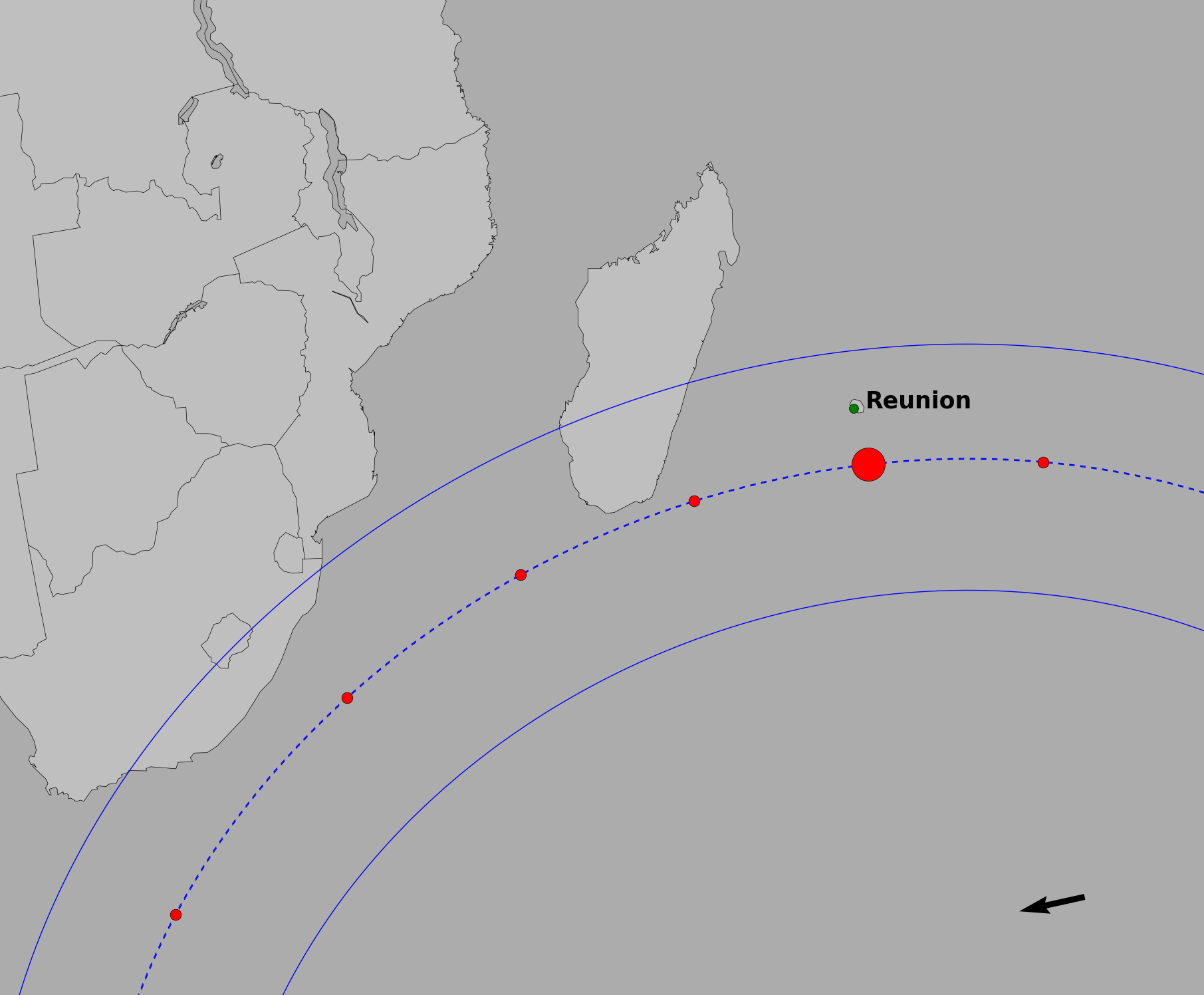
Figure 1: Post-occultation map for the December 12, 2013 occultation. North is up and East is right. Blue lines represent the object equivalent diameter from the November 07, 2014 occultation of 564.8 km. Red dots represent the position of the center of the body spaced every 30 seconds, the bigger dot corresponding to 20:10:44 UTC. Direction of the shadow is shown by the arrow at the right corner. Green dot is the site position with positive detection (see Table 4).

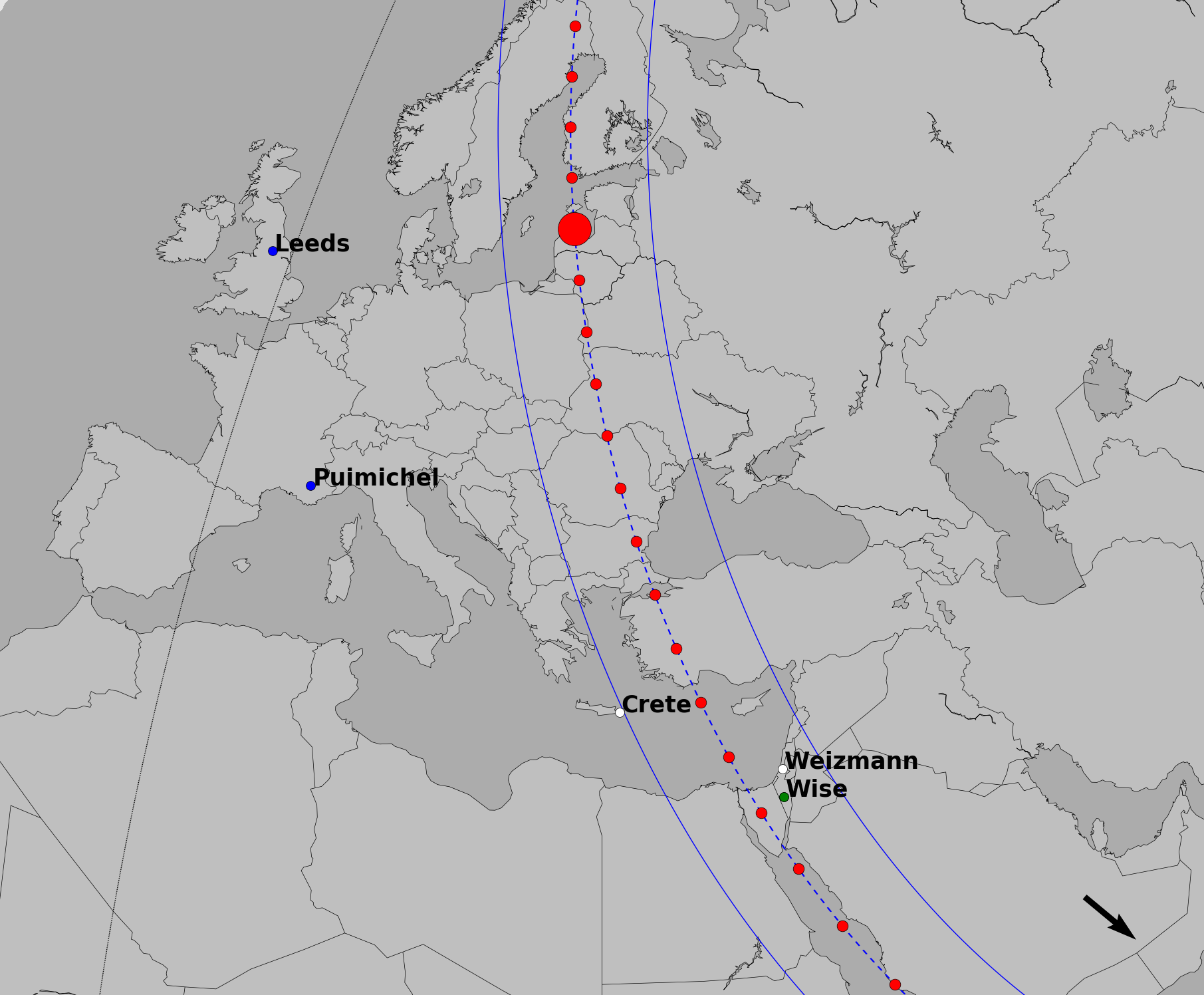
Figure 2: Post-occultation map for the March 04, 2014 occultation. North is up and East is right. Blue lines represent the object equivalent diameter from the November 07, 2014 occultation of 564.8 km. Red dots represent the position of the center of the body spaced every 30 seconds, the bigger dot corresponding to 19:55:54 UTC. Direction of the shadow is shown by the arrow at the right corner. Green dot is the site position with positive detection, while the blue dots are the negative detections and the white dots are the sites with weather overcast (see Table 4).

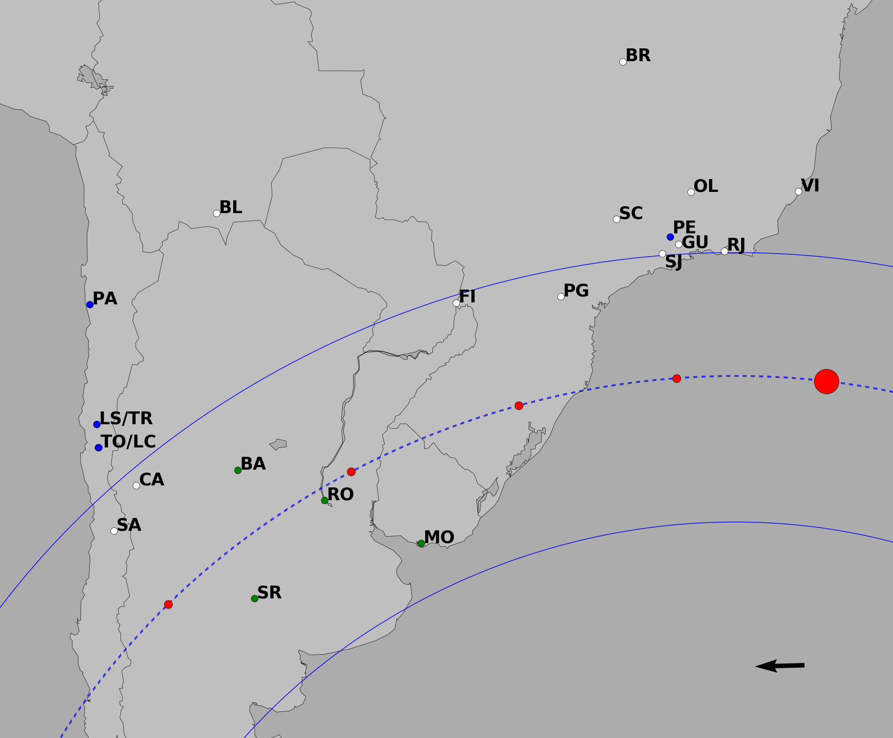
Figure 3: Post-occultation map for the November 07, 2014 occultation. North is up and East is right. Blue lines represent the object equivalent diameter obtained from this occultation, of 564.8 km. Red dots represent the position of the center of the body spaced every 30 seconds with the bigger one corresponding to 04:22:00 UTC. Direction of the shadow is shown by the arrow at the right corner. Green dots are the site positions with positive detections, while the blue dots are the negative detections and the white dots are the sites with weather overcast (see Tables 5 and 6).

Out of 23 stations distributed in nine countries (France, Israel, United Kingdom, Greece, Argentina, Uruguay, Chile, Brazil and Bolivia), we obtained two single-chord events and one multi-chord occultation, for a total of 7 positive detections. Note that the March 2014 occultation was detected by two telescopes at the same site in Israel. As such, they do not provide any constraint on the shape of the object, and we consider it as a single-chord detection. Figures 1, 2, and 3 show the post-occultation, reconstructed maps for the three events. Note that in those figures we used a radius for VS2 of 564.8 km (determined from the multi-chord occultation), but we do not know the rotational phase for the two single-chord occultations, so the shadow path may be smaller than this value. Details of data analysis for each occultation are given in Section 3.

Table 4: Observation details of the single-chord stellar occultations

December 12, 2013
Site Name	Longitude (E)	Telescope Aperture	Exposure Time
(Location)	Latitude (N)	Detector/Instrument	Cycle Time	Observers	Detection
$[$IAU Code$]$	Altitude (m)		(s)
Les Makes Observatory	55∘ 24’ 36.0”	60 cm	0.75000	J. Lecacheux
(La Réunion, France)	-21∘ 11’ 58.4”	Raptor Merlin 246	0.75031	A. Peyrot, T.-P. Baum	Positive
$[181]$	992			J.-P. Teng
March 04, 2014
Site Name	Longitude (E)	Telescope Aperture	Exposure Time
(Location)	Latitude (N)	Detector/Instrument	Cycle Time	Observers	Detection
$[$IAU Code$]$	Altitude (m)		(s)
Wise Observatory	34∘ 45’ 43.60”	100 cm	4
(Mitzpe Ramon, Israel)	30∘ 35’ 50.38”	Roper PVCAM	7	S. Kaspi	Positive
$[097]$	884	PI 1300B/LN
Wise Observatory	34∘ 45’ 43.92”	70 cm	5
(Mitzpe Ramon, Israel)	30∘ 35’ 48.23”	FLI	6.5	N. Brosch	Positive
$[097]$	865	PL16801
West Park Observatory	358∘ 23’ 31.98”	20 cm	5.08
(Leeds, UK)	53∘ 50’ 15.42”	WATEC	5.08	A. Pratt	Negative
$[Z92]$	114	WAT-910HX/RC (x256)	(video)
Puimichel Observatory	06∘ 01’ 15.5”	104 cm	0.25000	J. Lecacheux
(Puimichel, France)	43∘ 58’ 48.7”	Raptor Merlin 246	0.25031	S. Moindrot	Negative
–	724
Weizmann	34∘ 48’ 45.76”	41 cm	–
(Kraar, Israel)	31∘ 54’ 29.1”	SBIG	–	I. Manulis	Overcast
–	107	ST-8XME CCD
Sasteria Observatory	25∘ 58’ 16.37”	25 cm	–
(Crete, Greece)	35∘ 04’ 11.12”	N/A	–	F. Feys	Overcast
–	395

Note. — “FLI” stands for Finger Lakes Instruments; “PI” for Princeton Instruments; “PL” for Pro Line; “N/A” for Not Available.

Table 5: Observation details of the multi-chord stellar occultation on November 07, 2014 with data acquisition

Site Name	Longitude (E)	Telescope Aperture	Exposure Time
(Location)	Latitude (N)	Detector/Instrument	Cycle Time	Observers	Detection
$[$IAU Code$]$	Altitude (m)		(s)
Bosque Alegre	295∘ 27’ 01.5”	154 cm	5	C. A. Colazo
(Cordoba, Argentina)	-31∘ 35’ 54.0”	CMOS ZWO ASI120MM	5.000032	R. Artola	Positive
$[821]$	1213.1			R. Melia
Rosário	299∘ 21’ 09.0”	49 cm	3
(Rosário, Argentina)	-32∘ 58’ 16”	CCD KAF 8300	4	V. Buso	Positive
-	31.0
Montevideo	303∘ 48’ 37.1	46 cm	3	G. Tancredi
(Montevideo, Uruguay)	-34∘ 45’ 20.0”	FLI	4	S. Roland	Positive
-	130.0	PL9000		L. Almenares
				A. Ceretta
Santa Rosa	295∘ 40’ 32.5”	20 cm	25
(Santa Rosa, Argentina)	-36∘ 38’ 16.0”	CCD Meade DSI-I	26	J. Spagnotto	Positive
$[I48]$	182.0
ESO - VLT	289∘ 35’ 49.9’	400 cm	0.00664
(Cerro Paranal, Chile)	-24∘ 37’ 31.5”	HAWK-I	0.00667	V. D. Ivanov	Negative
$[309]$	2635.0
ESO - La Silla	289∘ 15’ 58.5’	355 cm	0.1	B. Sicardy
(La Silla, Chile)	-29∘ 15’ 32.3”	NTT/SOFI	0.10003	D. Bérard	Negative
$[809]$	2345.4.0
TRAPPIST-S	289∘ 15’ 38.2’	60 cm	3	C. Opitom
(La Silla, Chile)	-29∘ 15’ 16.6”	TRAPPIST-S	4.5	E. Jehin	Negative
$[I40]$	2317.7
PROMPT	289∘ 11’ 05.5”	40 cm	4
(Cerro Tololo, Chile)	-30∘ 09’ 56.3”	PROMPT	6	J. Pollock	Negative
$[807]$	2225.0
Las Cumbres*	289∘ 11’ 42.7”	100 cm	3/4
(Las Cumbres, Chile)	-30∘ 10’ 02.6”	FLI	5/6	F. Bianco	Negative
$[W85]$	2201.7	MicroLine 4720
		Dall Kirkham 50 cm	3	A. Maury	Negative
San Pedro de Atacama	291∘ 49’ 13.2”	Apogee U42	4
(S. P. de Atacama, Chile)	-22∘ 57’ 12”.1
$[I16]$	2398.50	Ash2 Newtonian 40 cm	15	N. Morales	Negative
		SBIG-STL11000	17.59
OPD/LNA	314∘ 25’ 03.0”	Perkin Elmer 160 cm	2	G. Benedetti-Rossi
(Itajubá, Brazil)	-22∘ 32’ 04”	Andor IXON	2.950	B. Morgado	Negative
$[874]$	1864.0	DU-888E-C00-#BV		A. R. Gomes-Junior	(w/ clouds)

Note. — “FLI” stands for Finger Lakes Instruments; “PI” for Princeton Instruments; “PL” for Pro Line. * Three 1-m telescopes were used at Las Cumbres (IAU codes W85, W86 and W87). One of them used I filter to minimize the moon contamination while the other two observed in Clear. Exposure time were 3 seconds for 2 telescopes (filters I and Clear) and 4 seconds for the third telescope. Readout time is not constant for this observation, but in average is 2 seconds. Computers are synchronized via NTP to the site GPS and the start of exposure in the three telescopes had a time shift in order to combine the three data sets and obtain one unique light curve without readout time.

Table 6: Observation details of the multi-chord stellar occultation on November 07, 2014 with no data acquired

Site Name	Longitude (E)	Telescope Aperture
(Country)	Latitude (N)	Detector/Instrument	Observers	Situation
	Altitude (m)
Brasília	312∘ 07’ 04.02”	G11 35 cm
(Brazil)	-15∘ 47” 40.37”	SBIG	P. Cacella	Overcast
	1096	ST8XMEI
Vitória (UFES)	319∘ 41’ 33.18”	GSO 35 cm
(Brazil)	-20∘ 16’ 41.43”	SBIG	M. Malacarne	Overcast
	6	ST8XME
Oliveira (SONEAR)	315∘ 10’ 27.88”	45 cm
(Brazil)	-20∘ 42 54.27	FLI	C. Jacques	Overcast
	984	16803
U. Autónoma Tomás Frías	295∘ 22’ 33.00”	Cassegrain 60 cm
(Bolivia)	-21∘ 35’ 45.90”	FLI	R. Condori	Overcast
	1866	IMG1001E
São Carlos (UFSCar)	312∘ 06’ 50.11”	Meade LX200 30 cm
(Brazil)	-21∘ 58’ 49.01”	SBIG	G. Rojas	Overcast
	847	ST9
Guaratinguetá (UNESP)	314∘ 48’ 29.50”	Meade LX200 40 cm
(Brazil)	-22∘ 48’ 10.02”	SBIG	R. Sfair	Overcast
	573	ST-7XME
Rio de Janeiro (ON)	316∘ 46’ 32,83”	Meade LX200 30 cm	F. Braga-Ribas
(Brazil)	-22∘ 53’ 46,85”	Raptor Merlin 246	J. I. B. Camargo	Overcast
	29
São José dos Campos (INPE)	314∘ 08’ 16”	C11 28 cm
(Brazil)	-23∘ 12’ 33”	SBIG	A. C. Milone	Overcast
	975	ST-7XE
Ponta Grossa (UEPG)	309∘ 53’ 41.39”	Meade RC40 40 cm
(Brazil)	-25∘ 05’ 40.27”	SBIG	M. Emilio	Overcast
	910	ST-6303E
Foz do Iguaçu	305∘ 24’ 22.55”	C11 28 cm
(Brazil)	-25∘ 26’ 05.45”	SBIG	D. I. Machado	Overcast
	185	ST-7XME
CASLEO	290∘ 41’ 15.9”	215 cm
(Argentina)	-31∘ 47’ 54.7”	PI-2048B	R. Gil-Hutton	Overcast
	2552
Montevideo	303∘ 48’ 37.1	Meade LX200 30 cm	G. Tancredi
(Uruguay)	-34∘ 45’ 20.0”	Raptor Merlin 246	S. Roland	Star not detected
	130.0		L. Almenares
			A. Ceretta

Note. — “FLI” stands for Finger Lakes Instruments; “PI” for Princeton Instruments.

2.3 Rotational light curve

In order to determine the rotational phase of VS2 at the time of the multi-chord occultation, we performed a photometric follow up of the object a few days after the event. We obtained a total of 97 images of VS2 over three nights – November 15, 16, and 17, 2014 – with the 2k $\times$ 2k CCD of the 1.5 m telescope at Sierra Nevada Observatory in Granada (Spain). The image scale of the instrument is 0.232 arcsec/pixel with a Field of View (FOV) of 7.92’ $\times$ 7.92’. All the images were acquired without filter and in 2 $\times$ 2 binning mode to maximize SNR. The integration time was 300 s throughout the three nights with a Moon illumination of 36% during the first night and 18% during the third night. The average seeing during the three nights was 3.3 arcsec. We pointed the telescope at the same coordinates on the three nights in order to use the same reference stars and thus minimize systematic photometric errors.

Standard Bias and Flat field corrections were applied on science images. Specific routines written in Interactive Data Language (IDL) were developed to perform the aperture photometry of all the chosen reference stars and VS2. We tried different apertures for the target, calibration stars and sky ring annulus in order to maximize the SNR on the object for each night and to minimize the dispersion of the photometry.

The flux of VS2 relative to the comparison stars is finally obtained versus the Julian Date, accounting for light travel times. The procedures we used were identical to those detailed in Fernández-Valenzuela et al (2016, 2017). We folded the final photometric data with the well-known rotational period for VS2 obtained in Santos-Sanz et al. (2017), P= 7.4175285 $\pm$ 0.00001 h. From this rotational light curve, we deduce that VS2 was near one of its absolute brightness maxima at the time of the November 07, 2014 stellar occultation (Fig. 4), which implies that the object occulted the star when its apparent surface area was near its maximum. These folded data are also fitted with a second order Fourier function in order to obtain the peak-to-valley amplitude of the rotational light curve, which turns out to be $0.141\pm 0.009$ mag (as listed in Table 10). The decrease in the peak-to-peak amplitude, compared to the value obtained by Thirouin et al. (2013), is probably due to geometric effects (i.e. a change in the aspect angle with respect to the previous amplitude estimations). The epoch for zero phase was chosen to be near the time of occultation (November 07, 2014 at 04:00:00 UTC).

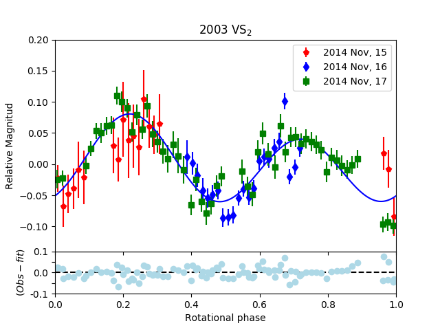
Figure 4: Rotational light curve for VS2 obtained on November 15 (in red), 16 (in blue) and 17 (in green), 2014 at Sierra Nevada Observatory (see text for details) just a few days after the occultation. Light blue dots on the bottom panel show the residuals between the observed points and the fit (blue line). The estimated rotational phase for the November 2014 stellar occultation is near one of the brightness maxima. We used the occultation date as the zero phase date.

3 Stellar Occultation Data Analysis

Some observations involved in the multi-chord event recorded only the integer part of the second in each image header. It was then necessary to retrieve the fractional part of the second for the mid-exposure time of each image by performing a linear fit to the set, see details in Sicardy et al. (2011) and Dias-Oliveira et al. (2017). From the linear fit we then retrieve the fraction of second for each image with an internal accuracy that depends on the square root of the number of images used, which is less than 0.1 s in practice.

Data obtained in video format from West Park Observatory was converted to Flexible Image Transport System (fits) format using the same procedure as described in Benedetti-Rossi et al. (2016) and Buie & Keller (2016).

The two single-chord events were analyzed to obtain the stellar flux (plus the faint, background contribution due to the occulting body) ratioed to nearby calibration stars using procedures based on the standard Daophot IDL routines (Stetson, P. B., 1987). The multi-chord occultation was harder to analyze. Since the SNR of the comparison and target stars were too low in all data sets, using the IDL routines the derived chords did not produce satisfactory results, as they presented sizes and positions that did not fit a reasonable and realistic ellipse in the sky plane. We then subjected the data sets to a careful treatment by the new photometry task version of PRAIA – Program for Reduction of Astronomical Images Automatically (Assafin et al., 2011).

PRAIA uses differential aperture photometry and it differs from the IDL routines in many instances, presenting many useful features which description is beyond the scope of this work. Among them, the apertures, sky ring sizes and widths are automatically optimized for better SNR (outside of the event) for each image, following a thorough aperture centering procedure, and the flux is precisely corrected for the variable apertures for all objects on each image. Calibration fluxes are smoothed and the best set of calibration stars is set automatically as a function of the best light curve standard deviation. The flux ratio vs. time is further corrected by atmospheric systematic factors (using the observed flux before and after the event) by applying a polynomial fit (we used the third degree in all cases). Finally, the flux ratio is normalized and the resulting normalized light curve stored with many kinds of information (errors, photometry parameters, etc). Note that the three stars magnitude are about 16, while it is almost 20 for the TNO. This means that VS2 is not visible in any of the equipment and exposures setup used in the observations and the stars disappear completely during the three occultations, with no residual light from VS2, i.e., we assume that the flux drops to zero in each of these observations. The resulting light curves with positive occultation detections are presented in Fig. 5. Light curves flux standard deviation are 21.8% for the 2013 occultation, 12.9% and 6.6% for the two telescopes of 0.7m and 1m, respectively, from the March 2014 event, while it is 6.9% for Bosque Alegre, 14.7% for Rosário, 14.5% for Santa Rosa, and 13.1% for Montevideo in the multi chord occultation.

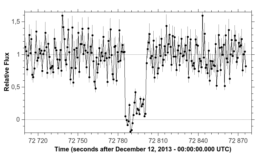
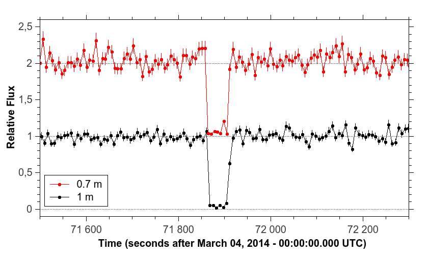
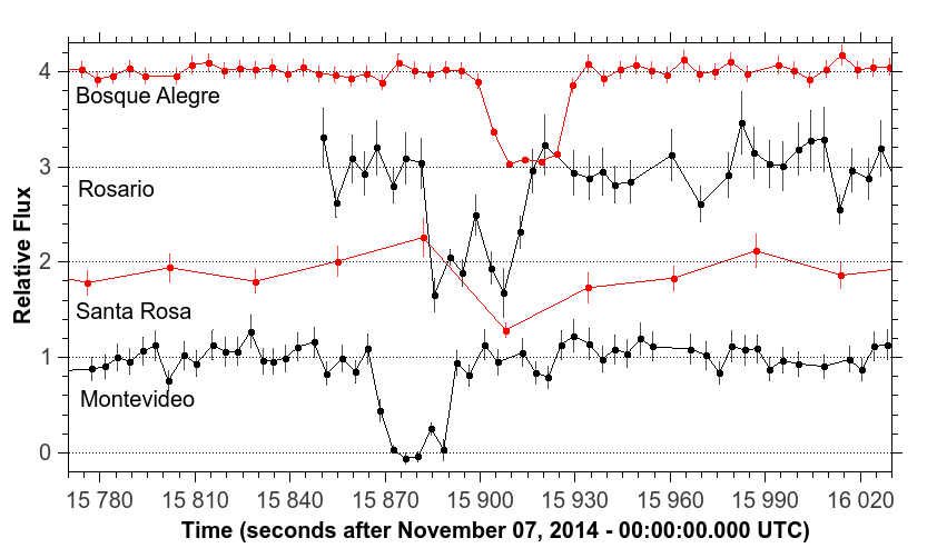
Figure 5: Normalized light curves of the positive detections of the stellar occultations – see Tables 4 and 5 for sites details. Top: single-chord event in December 12, 2013; Center: single-chord event in March 04, 2014, showing the detection with the two telescopes at the same site; Bottom: multi-chord event on November 2014. Chords are shifted in flux for better visualization. Vertical lines are the uncertainties in photometry for each point.

The start (star disappearance) and end (star reappearance) times of the occultation are determined by fitting each event by a sharp opaque edge model, after convolution by (i) Fresnel diffraction, (ii) finite CCD bandwidth, (iii) finite stellar diameter, and (iv) finite integration time (see details in Widemann et al. (2009); Braga-Ribas et al. (2013); Ortiz et al. (2017)). Note that the Fresnel monochromatic diffraction operates over the Fresnel scale $F=\sqrt{\lambda D/2}$, where $\lambda$ is the wavelength of observation and $D$ the geocentric distance of the object.

The stellar diameter projected at VS2’s distance is estimated using the B, V and K apparent magnitudes provided by the NOMAD catalog (Zacharias et al., 2004) and the formulae of van Belle (1999) – see Table 2. Using the apparent TNO motion relative to the star, it is possible to express the integration times in actual distances traveled between adjacent data points in the sky plane. Each effect is evaluated in Table 7. We note that our data are dominated by the integration times, and not by Fresnel diffraction or stellar diameter. The occultation timings are then obtained by minimizing a classical $\chi^{2}$ function, using the same procedures as described in Sicardy et al. (2011).

Table 7: Highest amplitude of effects to consider in order to determine the start and end instants of the three stellar occultations

Occultation Date	D 1	Fresnel 2	Star Diameter 3	Integration Time 4
	[au]	[km]	[km]	[km]
December 12, 2013	35.58	1.73	0.41	18.7
March 04, 2014	36.56	1.78	0.24	36.0
November 07, 2014	35.72	1.74	0.56	63.5

Note. — ¹ - Geocentric distance in astronomical units from Horizons/JPL (https://ssd.jpl.nasa.gov/horizons.cgi) using JPL#30 and DE431; ² - Fresnel diffraction effect ($F=\sqrt{\lambda D/2}$), see text; ³ - Stellar diameter projected at VS2’s geocentric distance calculated using (van Belle, 1999) and assuming super giant stars; ⁴ - The finite integration time is given for the smallest exposure time of the positive detections. It is expressed in kilometers after accounting for the velocity of the body projected in the sky plane, see text.

3.1 Single-chord events

The single-chord occultation of December 12, 2013 was detected from La Réunion Island and had a shadow velocity of 24.91 km s^-1, while the March 04, 2014 event had a shadow velocity of 8.99 km s^-1 and it was detected by two telescopes at the same site in Israel (see Table 4 for details). The best fits to the ingress and egress profiles are presented in Fig. 6. The occultation durations of 15.80${}^{+0.35}_{-0.40}$ s (La Réunion) and 45.75 $\pm$ 1.85 s (Israel) then correspond to occultation chords with lengths of 393.6${}^{+8.7}_{-10.0}$ km and 411.3 $\pm$ 16.6 km, respectively, see Table 8.

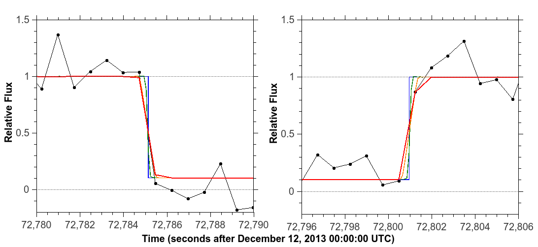
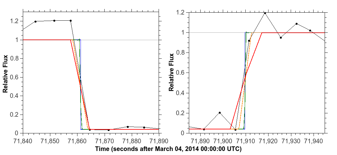
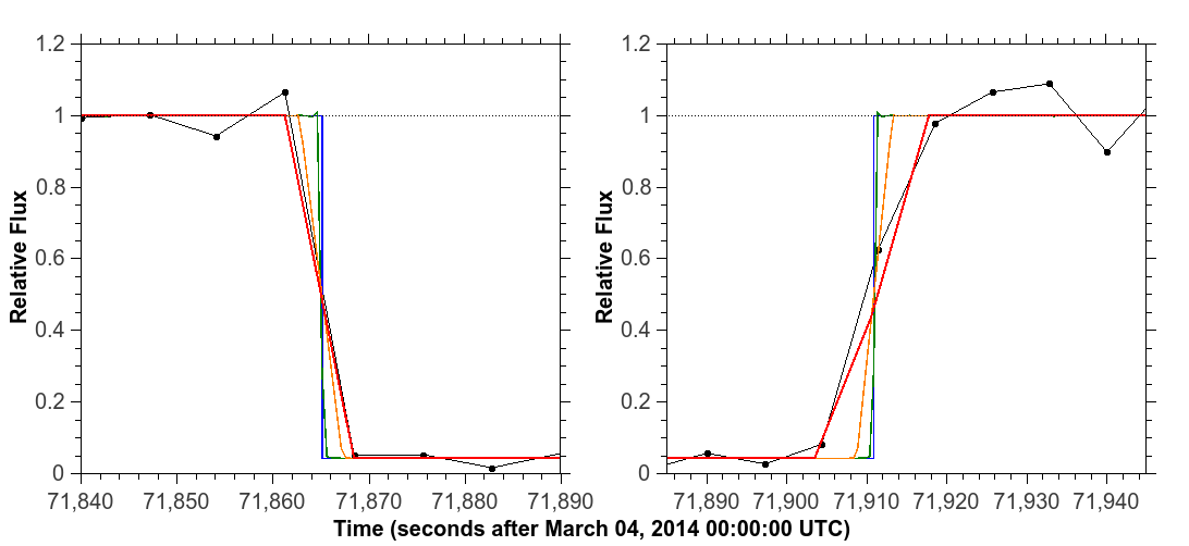
Figure 6: Best fit for the star disappearance (left) and reappearance (right) instants of the single-chord events – see Table 4 for sites details. Top: December 12, 2013 occultation; Center: March 04, 2014 occultation observed with the 0.7m telescope; Bottom: March 04, 2014 occultation observed with the 1m telescope. Data points are shown in black, the geometric square well models are in blue, the effect of diffraction is shown in green, the effect of finite integration time is added in the orange, and the red lines show all the effects accounted for, and then used for comparison with the actual data points.

The timings in Table 8 provide the extremities of the corresponding occultation chords projected in the sky plane. More precisely, they give the position $(f,g)$ of the star projected in the sky plane and relative to the center of the object. The quantities $f$ and $g$ are expressed in kilometers, and counted positively toward local celestial east and celestial north, respectively. Note that the calculated position $(f,g)$ depends on both the ephemeris used for the body and the adopted star position, that are both determined to within a finite accuracy. As such, $(f,g)$ must be corrected by an offset that can be determined if several chords are available, thus pinning down the position of the object’s center position relative to the star.

This is not possible for a single-chord event. In that case, a circle was adjusted to each chord, using the area-equivalent diameter of 564.8 km in order to determine the center of the TNO in the plane of the sky relative to the star at a prescribed time. Two solutions are then equally possible, depending on whether the center of the body went south or north of the star, as seen from Earth. We consider here the average of the two solutions, still resulting in an accurate astrometric positions for VS2 at the time of the two occultations, with uncertainties smaller than 25 mas for the two single-chord occultations. Note that the diameter used here was obtained from the November 07, 2014 occultation, when the object was at one of the maxima in brightness of the light curve, but we do not know the rotational phase for the other two single-chord occultations. This means that probably the shadow path must be smaller than 564.8 km. Anyway, a difference of 50 km in radius will give an uncertainty of less than 1.7 mas in the object position, which is within the error bars. The object positions in right ascension and declination corrected by the offsets obtained from the occultations are given in Table 9.

Table 8: Timings of star disappearances and reappearances

Occultation Event 1	Disappearance 2	Reappearance 2	Chord Size
	(s)	(s)	(km)
December 12, 2013	72785.15${}^{+0.15}_{-0.20}$	72800.95${}^{+0.15}_{-0.25}$	393.6${}^{+8.7}_{-10.0}$
March 04, 2014 (1m)	71865.15 $\pm$ 1.55	71910.9$\pm 0.3$	411.3 $\pm$ 16.6
March 04, 2014 (70cm)	71861.25 $\pm$ 1.15	71909.7${}^{+0.5}_{-0.6}$	435.6${}^{+14.8}_{-15.7}$
November 07, 2014 (BA)	15903.354 $\pm$ 0.646	15927.400 $\pm$ 0.642	517.7 $\pm$ 27.8
November 07, 2014 (RO)	15883.351 $\pm$ 0.887	15913.006 $\pm$ 0.670	638.5 $\pm$ 33.5
November 07, 2014 (SR)	15901.0 $\pm$ 8.0	15928.0 $\pm$ 8.0	581 $\pm$ 345
November 07, 2014 (MO)	15868.286 $\pm$ 0.800	15890.583 $\pm$ 0.800	480.1 $\pm$ 34.4

Note. — BA: Bosque Alegre; RO: Rosário; SR: Santa Rosa; MO: Montevideo; ¹ - See Tables 4, 5, and 6 for occultation details. ² - Times are given in seconds after 00:00:00.000 UTC of the occultation day.

Table 9: Astrometric right ascention and declination, and the offsets ($f,g$) for VS2 derived from the three stellar occultations

Occultation Date	RA ICRS	DEC ICRS	f *	g *
	(JPL30 and DE431 + Offset)		(mas)	(mas)
December 12, 2013 20:13:00.000	04h 36m 19s.83798	+33∘ 55’ 55”.2525	-15.7 $\pm$ 2.4	-17.5 $\pm$ 8.1
March 04, 2014 19:55:00.000	04h 32m 04s.47805	+33∘ 24’ 42”.0523	-12.2 $\pm$ 5.4	-23.7 $\pm$ 6.1
November 07, 2014 04:22:00.000	04h 48m 32s.13788	+33∘ 58’ 36”.1927	-60.1 $\pm$ 0.3	-24.5 $\pm$ 0.4

Note. — * The offsets depend also on the adopted star positions given on Table 2.

3.2 Multi-chord event

The November 07, 2014 occultation had a typical shadow velocity of 21.53 km s^-1 and observers attempted to record the event from 21 different sites. Unfortunately, due to bad weather only eight sites were successful in gathering data, among which four detected the event (see Tables 5 and 6). Despite non-detections, the chords obtained at Cerro Tololo (PROMPT), Las Cumbres, and La Silla (NTT/SOFI; Son of ISAAC (Moorwood et al., 1998a, b)) provide important constraints on the size of the object, being close to the occultation path.

The resulting light curves with positive detection, shown in Fig. 5, provide $N=8$ chord extremities, from which we derived the disappearance and reappearance instants of the occultation (see Table 8). The best fits for the ingress and egress times are presented in Fig. 7.

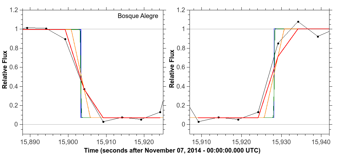
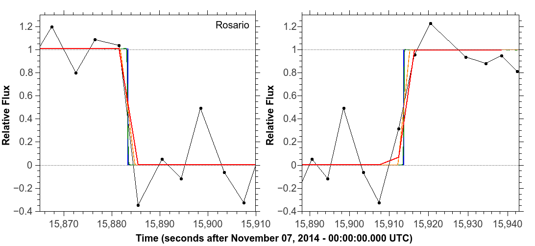
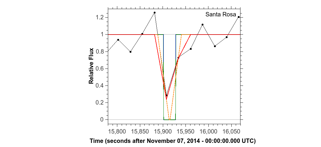
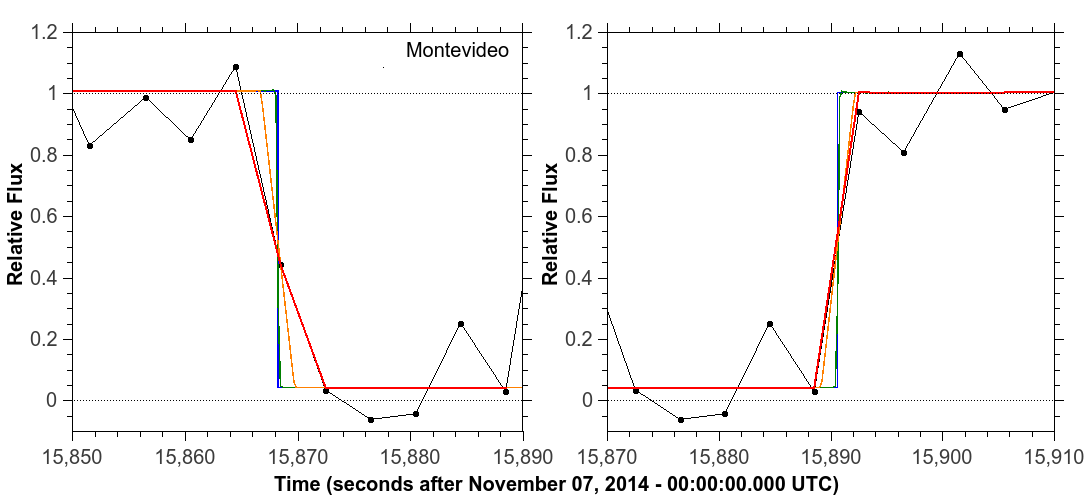
Figure 7: Best fit for the star disappearance (left) and reappearance (right) instants of the multi-chord event of November 07, 2014 – see Table 5 for sites details. From top to bottom: Bosque Alegre, Rosario, Santa Rosa, and Montevideo. Line colors are the same as in Fig. 6.

The shape of the body’s limb is assumed to be an ellipse, as adopted in previous works, see Braga-Ribas et al. (2013, 2014); Benedetti-Rossi et al. (2016); Dias-Oliveira et al. (2017); Ortiz et al. (2017). The ellipse is defined by $M=5$ adjustable parameters: the position of the ellipse center, $(f_{\rm c},g_{\rm c})$; the apparent semi-major axis, $a^{\prime}$; the apparent oblateness, $\epsilon^{\prime}=(a^{\prime}-b^{\prime})/a^{\prime}$ (where $b^{\prime}$ is the apparent semi-minor axis); and the position angle of the pole $P^{\prime}$ of $b^{\prime}$, which is the apparent position angle of the pole measured eastward from celestial north. Note that the center $(f_{\rm c},g_{\rm c})$ actually measures the offsets in right ascension and declination to be applied to the adopted ephemeris, assuming that the star position is correct. Note also that the quantities $a^{\prime}$, $b^{\prime}$, $f_{\rm c}$, and $g_{\rm c}$ are all expressed in kilometers.

The statistical significance of the fit is evaluated from the $\chi^{2}$ per degree of freedom (pdf) defined as $\chi^{2}_{pdf}$ = $\chi^{2}/(N-M)$, which should be close to unity for a correct fit. The individual 1-$\sigma$ error bar of each parameter is obtained by varying that parameter from its nominal solution value (keeping the other parameters free), so that $\chi^{2}$ varies from its minimum value $\chi^{2}_{\rm min}$ to $\chi^{2}_{\rm min}$ + 1.

Using the timings for the star disappearance and reappearance obtained from the four positive detections (Table 8), we obtain a best-fitting ellipse with $\chi^{2}_{pdf}=0.78$ and its parameters $a^{\prime}=313.8\pm 7.1$ km, $\epsilon^{\prime}=0.190^{+0.052}_{-0.060}$ ($b^{\prime}=254.8^{+25.0}_{-21.7}$), $(f,g)=(1558.1\pm 8.1,634.6\pm 11.0)$ km and $P^{\prime}=5\pm 7^{\circ}$, with equivalent radius $R_{\rm eq}=282.4^{+16.9}_{-15.1}$ km, as shown in Fig. 8.

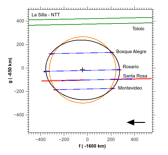
Figure 8: Occultation chords (blue) and their uncertainties (red) from the multi-chord event of November 2014 with the best elliptical fit (black). The offsets in both axis are with respect to ephemeride positions obtained using JPL#30 and DE431. The arrow shows the direction of the shadow motion and the green lines represent the two closest sites from where there were no detection of the occultation (see Table 5). The equivalent circle (that has the same area as the ellipse) is shown in orange with a diameter of 564.8 km.

4 Results

4.1 Size and Shape

Homogeneous rocky objects with diameters on the order of 1000 km or more are expected to have reached the hydrostatic equilibrium, assuming Maclaurin spheroidal or Jacobi ellipsoidal shapes (Chandrasekhar, 1987). The critical diameter allowing to reach this equilibrium is discussed by Tancredi & Favre (2008). In particular, hydrostatic equilibrium could be reached for smaller objects, if made of ices or of a combination of ices and rocks. Nevertheless, the formation scenario and collisional history of individual objects are not known, allowing objects with complex internal structures (i.e., differentiated density layers, granular for a peeble accretion scenario, etc.). Thus, we cannot discard solutions that diverge somewhat from the expected equilibrium figure given by Chandrasekhar (1987). The case of the dwarf planet Haumea (Ortiz et al., 2017) is a good example of a body with sizes that does not match a hydrostatic equilibrium figure for a geologically homogeneous fluid body.

The rotational light curve of Fig. 4 shows that VS2 is consistent with an object having a triaxial ellipsoidal shape. The short-term photometry of the body presented in Section 2.3 showed that the multi-chord occultation took place near one of the absolute brightness maxima of the rotational light curve, meaning that VS2 occulted the star when its apparent surface area was near its maximum. Assuming a triaxial shape, this occurs when its longest axis $a$ was perpendicular to the line of sight, so that the semi-major axis of the projected ellipse $a^{\prime}$ is equal to the real 3D-axes. With the known rotation period and phase, we verified if it was possible to use one or the two single-chord occultation results to improve the accuracy on the determination of size and shape for the TNO. The problem is that even if the rotational phase and period are well determined, the ephemeris for the object is not well constrained, with uncertainties of about 50 mas, in a way that the chord from the two occultations can fit anywhere in the multi-chord apparent ellipse. With this uncertainty we could not use any of the other chords to obtain further constraints on VS2’s shape using the same method that Dias-Oliveira et al. (2017) did for the TNO 2003 AZ₈₄.

Considering the limb fit to the apparent ellipse obtained from the multi-chord occultation and the light curve amplitude, we can use the same procedure as in Sicardy et al. (2011) (also used in Braga-Ribas et al. (2013) and Ortiz et al. (2017)) to derive the three axes of the body. Our best solution for a triaxial shape has semi-axis values $a=313.8\pm 7.1$ km, $b=265.5^{+8.8}_{-9.8}$ km ($\beta=0.846^{+0.031}_{-0.028}$), $c=247.3^{+26.6}_{-43.6}$ km ($\gamma=0.788^{+0.085}_{-0.139}$), with the c-axis inclined $\theta=65^{+15}_{-10}~{}^{\circ}$ with respect to the observer, which is not consistent with the Jacobi equilibrium figure – see Appendix A for details. This solution gives a spherical volume equivalent diameter of $548.3^{+29.5}_{-44.6}$, from which we can derive (using H_v = 4.130 $\pm$ 0.070 mag) the geometric albedo $p_{V}=0.131^{+0.024}_{-0.013}$.

Since we can not make any constraint about VS2’s density using the triaxial approach without making any other assumption of its mass, we can make an assumption that VS2 has an oblate shape, as a Maclaurin equilibrium figure with semi-axis $a=313.8$ km and $254.8\leq c\leq 313.8$ km. Note that with this assumption, we are also assuming that the light curve amplitude variation is due to albedo features. Making this assumption and combining with the rotation period (given in Table 1), we can derive its density of $1400^{+1000}_{-300}$ kg m^-3. All those values are summarized in Table 10.

Table 10: Solution for 2003 VS₂ derived from the multi-chord stellar occultation and the rotational light curve.

Parameter	Value
$a^{\prime}\times b^{\prime}$ (km)	$313.8\pm 7.1\times 254.8^{+25.0}_{-21.7}$
($f,g$) (km) 1	(-1558.1 $\pm$ 8.1 ; -634.6 $\pm$ 11.0)
Position angle of projected ellipse (deg)	$5\pm 7$
Light curve amplitude 2 – $\Delta m$ – (mag)	0.141 $\pm$ 0.009
Geometric albedo – $p_{V}$	$0.131^{+0.024}_{-0.013}$.
$a\times b\times c$ (km)	$313.8\pm 7.1\times 265.5^{+8.8}_{-9.8}\times 247.3^{+26.6}_{-43.6}$
Aspect angle (deg)	$65^{+15}_{-10}$
Equivalent diameter (km)	$548.3^{+29.5}_{-44.6}$
Density – Maclaurin (kg m-3)	$1400^{+1000}_{-300}$

Note. — ¹ Offsets obtained with respect to JPL30 + DE431. It also depends on the star position given in Table 2.² Period used to fit was 7.4175285 $\pm$ 0.00001 h from Santos-Sanz et al. (2017).

4.2 Atmosphere and secondary detections

On the largest TNOs the most common volatiles found through spectroscopic studies are water ice (H₂O), methane (CH₄), ammonia (NH₃), molecular nitrogen (N₂), and even methanol (CH₃OH) and ethane (C₂H₆) for a few objects (Guilbert et al., 2009; Barucci et al., 2011). In the case of VS2, near infrared spectra of this body shows the presence of exposed water ice (Barkume et al., 2008), but no other volatile is reported to be detected. Data from the three stellar occultations showed no compelling evidence for a global atmosphere.

Using the same method for Quaoar (Braga-Ribas et al., 2013), we have modeled synthetic occultation light curves using a ray tracing code as described in Sicardy et al. (2011) and Widemann et al. (2009). Several synthetic light curves are then compared to our best light curve obtained at Wise Observatory on the single chord occultation on March 04, 2014 providing a range of $\chi^{2}$ with the detection threshold. We test two possible atmospheric models. one with an isothermal N₂ atmosphere, as this gas is the most volatile one among those listed above. We consider a typical temperature of 40 K for this model, but the result is weakly dependent on this particular value. The other model is a N₂ atmosphere with CH₄ as a minor species, starting near 40 K at the surface and ramping up to 100 K near 25 km altitude due to methane IR absorption, as is observed in Pluto’s atmosphere (Hinson et al., 2017).

Our $\chi^{2}$-tests show that for both models, the Wise data are consistent with no atmosphere, with upper limits of 0.2 microbar and 1 microbar at the 1$\sigma$ and 3$\sigma$ levels, respectively.

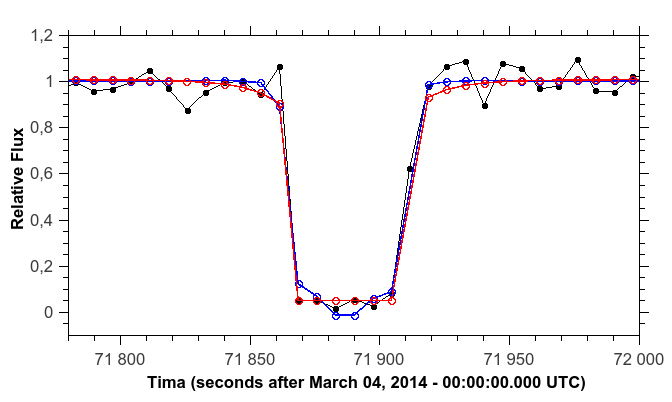
Figure 9: Light curve from the single-chord stellar occultation of March 04, 2014 obtained at Wise Observatory (black) and the two models for the isothermic pure nitrogen (red) and a Pluto-like (blue) atmospheres within a 3$\sigma$ limit.

We also searched for secondary events that may be related to a satellite, ring, or some material orbiting VS2. Using our highest time-resolution light curve – obtained with the 3.5m NTT telescope with 0.1 seconds of cycle time and roughly positioned 400 km from VS2’s center – we can estimate an upper limit of 0.2 km for an opaque object (or 18.5 km for any material with optical depth of 0.1). Considering the best chord with positive detection – from Bosque Alegre with 5 seconds cycle time – those limits are 107.7 km for opaque and 732 km for material with optical depth of 0.1.

One secondary feature was also detected in the NTT light curve, as shown in Fig. 10. The drop has a relative depth of less than 10% (compared to the light curve standard deviation of 8.6%) and a duration of about 29 s, corresponding to a chord length of 625 km. However, this drop remains marginally significant and cannot be confirmed or rejected using the nearby chords from Cerro Tololo (insufficient SNR) and Pico dos Dias (overcast). This drop could be due to an occultation of a companion star by the object, causing a secondary occultation as happened during a stellar occultation by the Centaur object Chariklo in 2014 – see Leiva et al. (2017) and Bérard et al. (2017). Note that with the size of VS2 and the geometry of the occultation, the Bosque Alegre positive light curve (data set with the best SNR) should not present any sign of this possible secondary occultation. Also, considering the main star magnitude (V=15.82) and the drop of 10%, the companion would have a magnitude V=18.21. If this star is closer than 0.8 arcsec it is likely not to be present in the GDR2 catalog (Brandeker & Cataldi, 2019). We estimate that the companion star should be closer than 0.5 arcsec, so the existence of a stellar companion remains consistent with its absence in the GDR2.

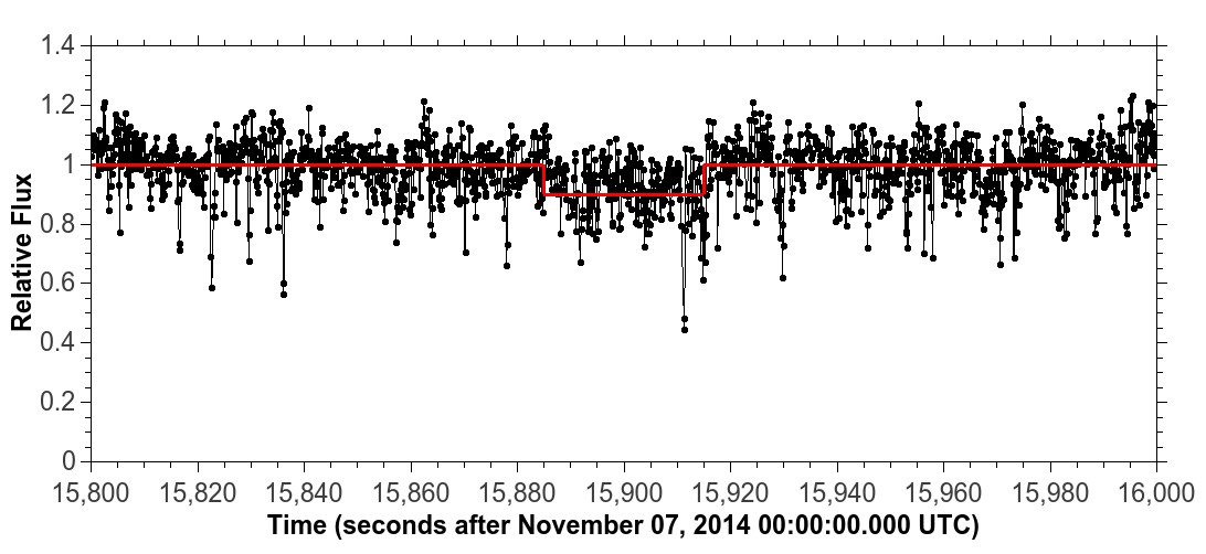
Figure 10: Light curve from the multi-chord stellar occultation of November 07, 2014 obtained at La Silla/NTT. All the flux drops in the curve are due to the star being too close to the edge of the CCD or being influenced by the bad row of pixels in the center of the CCD. Note the relative flux drop of 0.09 that happens between instants 15885 s and 15915 s, fitted using a square well model, represented by the red line.

Another possibility is that this drop is due to some diffuse material around VS2, but since none of the other light curves show such secondary event to within the 5-$\sigma$ level, this hypothesis is less likely. Also, a careful look on the NTT images presents some issues. The images have 320 vs. 32 pixels with a dead row in the middle of the CCD (row 69). There was only one reference star in the field for photometric calibration, which is fainter than the occulted star, and the telescope tracking was not perfect, in a way that sometimes one or both stars were close to the edge of the CCD. So we can not completely discard instrumental effects or reduction artifacts on this data set. In conclusion, more occultations are needed in order to confirm or discard the presence of any secondary feature.

5 Conclusions

We observed two single-chord and one multi-chord stellar occultations by the plutino (84922) 2003 VS₂. Observations were performed on December 12, 2013 in La Réunion, on March 04, 2014 in Israel, and from 11 sites in South America on November 07, 2014, with 4 positive detections. The two single-chord events are consistent with the multi-chord solutions but do not bring further constraints to the object shape. However, they provide good astrometric constraints, thus improving the ephemeris of the body.

Using the timings of the November 07, 2014 event, we find the apparent ellipse with area equivalent diameter of 564.8${}^{+33.8}_{-30.2}$ km. Assuming that VS2 has a triaxial shape and combining the occultation data with the light curve amplitude ($\Delta m=0.141\pm 0.009$) obtained from photometric observations of the TNO, we derive the object 3D-shape, with semi-axes $a=313.8\pm 7.1$ km, $b=265.5^{+8.8}_{-9.8}$ km, $c=247.3^{+26.6}_{-43.6}$ km, with the c-axis inclined $\theta=65^{+15}_{-10}~{}^{\circ}$ with respect to the observer. Those values are not consistent with a Jacobi equilibrium figure, but are in accordance, at the 1-$\sigma$ level, with previous values published by Mommert et al. (2012), Stansberry et al. (2008), and Lellouch et al. (2013) (area equivalent diameter of 523${}^{+35.1}_{-34.4}$ km).

We also considered the possibility that VS2 is an oblate Maclaurin equilibrium figure (with $a=b>c$). With this assumption, the light curve amplitude variation is due to albedo features and VS2 would have a density of $\rho=1400^{+1000}_{-300}$ kg m^-3. The light curve amplitude can be explained in the extreme cases to be due only to the shape (with the triaxial shape model) or to a darker or brighter spot on the surface of about 100 km – 16% of object diameter – if VS2 is a Maclaurin.

A possible secondary event was detected in the NTT data, that may be caused by the presence of some feature in VS2’s surroundings or due to a secondary occultation occurred by the presence of a companion star, but the data are insufficient to make any deep conclusions. We also derived an upper limit for a global atmosphere (either isothermic pure nitrogen or Pluto-like) of 1 microbar (3$\sigma$).

Although the rotation period is well defined, and values for the geometric albedo and size of VS2 are well determined with the occultations, its 3D-shape (and as a consequence, its density) still need more observations in order to constrain the values obtained in this work.

Appendix A Deriving VS2’s shape and Density

We describe here the procedure used to determine the values of the semi-axis of a triaxial ellipsoid ($a>b>c$), and the angle between the c-axis and the observer ($\theta$).

First we have the relations from Sicardy et al. (2011) (also used in Braga-Ribas et al. (2013) and Ortiz et al. (2017)) between the real $c$ and $b$ semi-minor axis and the observed $b^{\prime}$:

$$b^{\prime}=\sqrt{c^{2}~{}sin^{2}\theta+b^{2}~{}cos^{2}\theta},$$ (A1)

where in our case we have $b^{\prime}=254.8^{+25.0}_{-21.7}$ km as the semi-minor axis of the ellipse observed in occultation. Multiplying both sides by $1/a$ and replacing $b/a$ by $\beta$, and $c/a$ by $\gamma$, we can rewrite eq. A1 and rearrange the terms to have a direct relation of $\gamma$ as a function of $\beta$:

$$\gamma^{2}={\frac{\beta^{\prime 2}-\beta^{2}cos^{2}\theta}{sin^{2}\theta}}$$ (A2)

Note that since the multi-chord occultation took place near the maximum brightness, we have $a^{\prime}=a$, and so $\beta^{\prime}=b^{\prime}/a$. Second, using equation (8) from Sicardy et al. (2011) (SI) we have

$$\Delta m=-1.25\cdot\log_{10}{\left[\frac{1+\gamma^{2}\tan^{2}{\theta}}{1+(\gamma/\beta)^{2}\tan^{2}{\theta}}\right],}$$ (A3)

where $\Delta m$ is the amplitude of the rotational light curve (0.141 $\pm$ 0.009 mag – see Table 1). We can rearrange the terms in the equation and obtain another relation of $\gamma$ as function of $\beta$:

$$\gamma^{2}=\frac{\beta^{2}~{}(\xi-1)}{tg^{2}\theta~{}(\beta^{2}-\xi)},$$ (A4)

where $\xi=10^{-\Delta m/1.25}$. Those two equations combined (eqs. A2 and A4) give us constraints on the values $\beta$ for every $\theta$, but without any further assumptions, $\gamma$ can assume any value from zero (or more specifically, undefined) to $\beta$ and $\theta$ can have values from $0$ to $90$ degrees.

Now, assuming that VS2 is large enough to achieve hydrostatic equilibrium, we have the limits for $\beta$ and $\gamma$ as a Jabobi-shape object. Tancredi & Favre (2008) present the relations $\Gamma$ – associated with the angular momentum $L$ – and $\Omega$ – associated with the angular velocity $\omega$ – given respectively by:

$$\Gamma=\frac{L}{\sqrt{GM^{3}R}},$$ (A5)

and

$$\Omega=\frac{\omega^{2}}{\pi G\rho},$$ (A6)

where $G$ is the gravitational constant, $M$, $R$, and $\rho$ are the mass, equivalent radius and density of the body, respectively. For a Jacobi object, there are a lower and an upper limit for the two quantities: $0.303\leq\Gamma\leq 0.390$, and $0.284\leq\Omega\leq 0.374$; which also limit the values of $\beta$ between 0.432 and 1, and $\gamma$ between 0.345 and 0.583. The shapes of Jacobi ellipsoids in terms of the semi-axes ($a,b$, and $c$) can only be obtained by solving Chandrasekhar (1969) – also in Lacerda & Jewitt (2007) and Sicardy et al. (2011) Suplemmentary Information – integrals:

$$\beta^{2}\int_{0}^{\infty}\frac{du}{(1+u)~{}(\beta^{2}+u)~{}\Delta(\beta,\gamma,u)}=\gamma^{2}\int_{0}^{\infty}\frac{du}{(\gamma^{2}+u)~{}\Delta(\beta,\gamma,u)}$$ (A7)

and

$$\frac{\omega^{2}a^{3}}{GM}=\frac{3}{2}\int_{0}^{\infty}\frac{u~{}du}{(1+u)~{}(\beta^{2}+u)~{}\Delta(\beta,\gamma,u)},$$ (A8)

where $\Delta(\beta,\gamma,u)=[(1+u)~{}(\beta^{2}+u)~{}(\gamma^{2}+u)]^{1/2}$. Once $\beta=b/a$ is given, Eq. A7 yields $\gamma$, which in turn allows to calculate $\omega$ (or $\rho$), using Eq. A8.

We can plot the two relations between $\gamma$ and $\beta$ for a triaxial body (eq. A2 is represented in Fig. 11 and eq. A4 in Fig. 12) and verify if there exists a set of possible common solutions for every value of $\theta$. Each of the intersections between the two curves for a same $\theta$ are presented in grey line in Fig. 13. If we also plot the Jacobi relation between $\gamma$ and $\beta$ (blue line in Fig. 13) we should see a solution that intersects the three curves, which is not the case for VS2. This means that there is a solution for a triaxial shape but this solution is not a Jacobi shape.

In the case of VS2 the best solution for a triaxial shape have values for $\theta=65^{+15}_{-10}$ degrees, with $\beta=0.846^{+0.031}_{-0.028}$ ($b=265.5^{+8.8}_{-9.8}$ km), $\gamma=0.788^{+0.085}_{-0.139}$ ($c=247.3^{+26.6}_{-43.6}$ km). Those values are also given on Table 10.

In order to have a Jacobi solution, we can explore different values for $\Delta m$, from 0 to the nominal value of 0.141 mag. In fact we are assuming that some of the light curve contribution is due to VS2’s shape and some due to albedo variation in the surface. When we try values for $\Delta m$ smaller than 0.141 the lines in Fig. 12 will move to the right and so more intersections with the lines from Fig. 11 will be available, i.e., there will be an intersection between the grey and the blue lines in Fig. 13. For $\Delta m=0.015$ mag we find a Jacobi solution with $\beta=0.908$ ($b=284.9$ km), $\gamma=0.553$ ($c=173.5$ km) and $\theta=75~{}^{\circ}$.

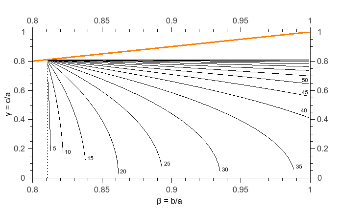
Figure 11: Relation between $\beta=b/a$ and $\gamma=c/a$ obtained using eq. A2. Black lines correspond to a value of $\theta$ between 5 and 90 degrees (from left to right), every 5 degrees. Orange line are the values for $\beta=\gamma$. Red dotted vertical line is the value of $\beta^{\prime}=0.811$, observed in occultation.

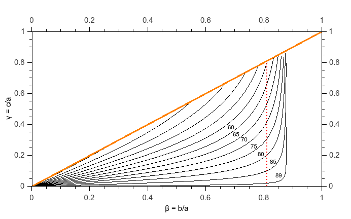
Figure 12: Relation between $\beta=b/a$ and $\gamma=c/a$ obtained using eq. A4. Black lines correspond to a value of $\theta$ between 0 and 90 degrees (from left to right), every 5 degrees. Orange line are the values for $\beta=\gamma$. Red dotted vertical line is the value of $\beta^{\prime}=0.811$, observed in occultation.

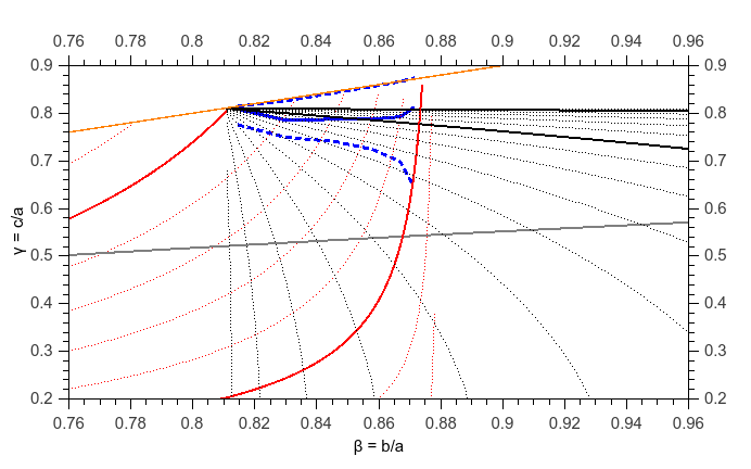
Figure 13: Relation between $\beta=b/a$ and $\gamma=c/a$ combining eq. A2 (black dotted lines – as in Fig. 11) and eq. A4 (red dotted lines – as in Fig. 12). Blue curve is the intersection between the black and red lines for each value of $\theta$ and the uncertainties (dotted blue lines – which depends on the determination of $\beta^{\prime}$ and $\Delta m$). The orange line is the value for $\beta=\gamma$ while the grey line represents the relation for $\beta$ and $\gamma$ for the Jacobi shape. For $\theta$ between 55 and 80^∘, defined by the black and red full lines, there is no intersection between the blue and grey lines, meaning that there is no Jacobi solution for VS2.

We can also explore the other extreme and assume that VS2 has an oblate Maclaurin shape (with semi-axis $a=b=313.8\pm 7.1$ km and $254.8\leq c\leq 313.8$ km). This assumption automatically imposes that the light curve amplitude variation is only due to albedo features on VS2’s surface. Considering the light curve amplitude of 0.141 $\pm$ 0.009 mag – see Table 1 – the presence of surface irregularities (lumps) and some albedo variegation (spots) on the object with a size approximately of 100 km ($\sim 16\%$ of the object equivalent area) is needed. Note that the Sputnik Planitia in Pluto is nearly 1000 x 800 km across ($\sim 15\%$ of its equivalent area) (Hamilton et al., 2016). Considering the Maclaurin shape and using the rotational period (P = 7.4175285 $\pm$ 0.00001 h – see Table 1), we can derive VS2’s density of $\rho=1.4^{+1.0}_{-0.3}$ g cm^-3, as show in Fig. 14.

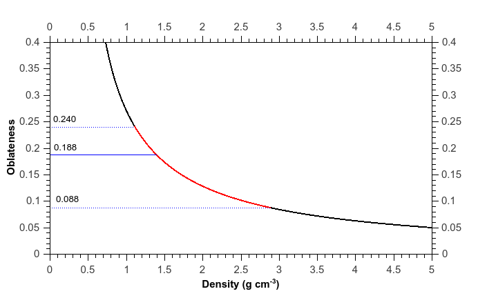
Figure 14: Relation between $\epsilon$ and density for a Maclaurin object with rotation period of 7.4175285 hours (black line). The oblateness obtained for VS2 (blue horizontal full and dotted lines) gives limits for the minimum value of the density of 1.4 g cm^-3. Blue dotted lines represent the values considering the uncertainties in $a$ and $b$. Red line is the interval between the limits.

References

- Alvarez-Candal et al. (2016) Alvarez-Candal, A.; Pinilla-Alonso, N.; Ortiz, J. L.; et al., 2016, A&A, V. 586, id.A155
- Anglada et al. (2017) Anglada, G., Amado, P. J., Ortiz, J. L., et al., 2017, ApJ, 850, L6
- Assafin et al. (2010) Assafin, M.; Camargo, J. I. B.; Vieira Martins, R.; et al., 2010, A&A, V. 515
- Assafin et al. (2011) Assafin, M.; Vieira-Martins, R.; Camargo, J. I. B.; et al., 2011, GAIA FUN-SSO workshop proccedings, 85, gfun.conf
- Assafin et al. (2012) Assafin, M.; Camargo, J. I. B.; Vieira Martins, R.; et al., 2012, A&A, V. 541
- Barkume et al. (2008) Barkume, K. M.; Brown, M. E.; & Schaller, E. L., 2008, AJ, V. 135
- Barucci et al. (2011) Barucci, M. A.; Dotto, E. & Levasseur-Regourd, A. C., 2011, A&A Rev., V.19, id.48
- Belskaya et al. (2006) Belskaya, I. N.; Ortiz, J. L.; Rousselot, P.; et al., 2006, Icarus, V. 184, Issue 1
- Benedetti-Rossi et al. (2016) Benedetti-Rossi, G.; Sicardy, B.; Buie, M. W.; et al., 2016, AJ, V. 152, Issue 6, id. 156
- Bérard et al. (2017) Bérard, D.; Sicardy, B.; Camargo, J. I. B.; et al., 2017, AJ, V. 154, Issue 4, id. 144
- Binzel et al. (1989) Binzel, R. P.; Farinella, P.; Zappala, V. & Cellino, A., 1989, in Asteroids II (eds Binzel, R. P. et al.), 416–441, Univ. Arizona Press.
- Braga-Ribas et al. (2013) Braga-Ribas, F.; Sicardy, B.; Ortiz, J. L.; et al., 2013, ApJ, 773, id. 26
- Braga-Ribas et al. (2014) Braga-Ribas, F.; Sicardy, B.; Ortiz, J. L.; et al., 2014, Nature, 508, 7494
- Brandeker & Cataldi (2019) Brandeker & Cataldi, 2019, A&A, 621, A86
- Buie & Keller (2016) Buie, M. W.; Keller, J. M., 2016, AJ, V. 151, Issue 3
- Camargo et al. (2014) Camargo, J. I. B.; Vieira-Martins, R.; Assafin, M.; et al., 2014, A&A, V. 561, id.A37
- Camargo et al. (2018) Camargo, J. I. B.; Desmars, J.; Braga-Ribas, F., et al., 2018, Planet. Space Sci., V. 154, p. 59-62
- Chandrasekhar (1969) Chandrasekhar, S., 1969, Ellipsoidal Figures of Equilibrium, The Silliman Foundation Lectures, New Haven: Yale University Press
- Chandrasekhar (1987) Chandrasekhar, S., 1987, Ellipsoidal Figures of Equilibrium (New York: Dover)
- Deeths & Brunette (2001) Deeths, D. & Brunette, G., 2001, in Using NTP to Control and Synchronize System Clocks Part I: Introduction to NTP (Sun BluePrintsTM), OnLine 2001 July
- Dias-Oliveira et al. (2017) Dias-Oliveira, A.; Sicardy, B.; Ortiz, J. L.; et al., 2017, AJ, V. 154, id. 22
- Duffard et al. (2008) Duffard, R.; Ortiz, J. L.; Santos Sanz, P.; et al., 2008, A&A, V. 479, Issue 3
- Fernández-Valenzuela et al (2016) Fernández-Valenzuela, E.; Ortiz, J. L.; Duffard, R.; et al., 2016, MNRAS, 456, Issue 3
- Fernández-Valenzuela et al (2017) Fernández-Valenzuela, E.; Ortiz, J. L.; Duffard, R.; et al., 2017, MNRAS, 466, Issue 4
- Gaia Collaboration (2016a) Gaia Collaboration; Brown, A. G. A.; Vallenari, A.; et al., 2016, A&A, V. 595, A2
- Gaia Collaboration (2016b) Gaia Collaboration; Prusti, T.; de Bruijne, J. H. J.; et al., 2016, A&A, V. 595, A1
- Gaia Collaboration (2018) Gaia Collaboration; Brown, A. G. A.; Vallenari, A.; et al., 2018, eprint arXiv:1804.09365
- Gladman et al. (2008) Gladman, B.; Marsden, B. G. & Vanlaerhoven, C., 2008, in The Solar System Beyond Neptune, M. A. Barucci, H. Boehnhardt, D. P. Cruikshank, and A. Morbidelli, University of Arizona Press
- Guilbert et al. (2009) Guilbert, A.; Alvarez-Candal, A.; Merlin, F. et al., 2009, Icarus, V. 201, Issue 1
- Hamilton et al. (2016) Hamilton, Douglas P.; Stern, S. A.; Moore, J. M. et al., 2016, Nature, V. 540, Issue 7631, pp. 97-99
- Hinson et al. (2017) Hinson, D. P., Linscott, I. R., Young, L. A., et al., 2017, Icarus, 290, 96
- Jewitt & Luu (1993) Jewitt, D. & Luu, J., 1993, Nature, 362, 6422
- Jewitt et al. (2008) Jewitt, D.; Morbidelli, A. & Rauer, H., 2008, in Trans-Neptunian Objects and Comets, Saas-Fee Advanced Course 35, 2008, XII
- Lacerda & Jewitt (2007) Lacerda, P.; Jewitt, D. C., 2007, AJ, V. 133, Issue 4, pp. 1393, id. 159
- Leiva et al. (2017) Leiva, R.; Sicardy, B.; Camargo, J. I. B.; et al., 2017, AJ, V. 154, Issue 4, id. 159
- Lellouch et al. (1986) Lellouch, E.; Hubbard, W. B.; Sicardy, B.; et al., 1986, Nature, V. 324, Nov. 20, 1986, p. 227-231
- Lellouch et al. (2002) Lellouch, E.; Moreno, R.; Ortiz, J. L.; et al., 2002, A&A, V. 391
- Lellouch et al. (2013) Lellouch, E.; Santos-Sanz, P.; Lacerda, P.; et al., 2013, A&A, V. 557
- Lykawka & Mukai (2008) Lykawka, P. S.; Mukai, T., 2008, AJ, 135, 4, 1161-1200
- MPEC (2006) Minor Planet Center Electronic Circular 2006-X45
- Mommert et al. (2012) Mommert, M.; Harris, A. W.; Kiss, C.; et al., 2012, A&A, V. 541, A93
- Moorwood et al. (1998a) Moorwood, A.; Cuby, J.-G.; Biereichel, P.; et al., 1998, The Messenger, V. 94, p. 7-9
- Moorwood et al. (1998b) Moorwood, A.; Cuby, J.-G.; Lidman, C., 1998, The Messenger, V. 91, p. 9-13V
- Morbidelli et al. (2008) Morbidelli, A.; Levison, H. F.; & Gomes, R., 2008, in The Solar System Beyond Neptune, M. A. Barucci, H. Boehnhardt, D. P. Cruikshank, and A. Morbidelli, University of Arizona Press, Tucson
- Ortiz et al. (2002) Ortiz, J. L.; Baumont, S.; Gutiérrez, P. J.; et al., 2002, A&A, V. 388
- Ortiz et al. (2004) Ortiz, J. L.; Sota, A.; Moreno, R.; et al., 2004, A&A, V. 420
- Ortiz et al. (2006) Ortiz, J. L.; Gutiérrez, P. J.; Santos-Sanz, P.; et al., 2006, A&A, V. 447, Issue 3
- Ortiz et al. (2007) Ortiz, J. L.; Santos Sanz, P.; Gutiérrez, P. J.; et al., 2007, A&A, V. 468, Issue 1
- Ortiz et al. (2011) Ortiz, J. L.; Cikota, A.; Cikota, S.; et al., 2011, A&A, V. 525, id. A31
- Ortiz et al. (2012) Ortiz, J. L.; Sicardy, B.; Braga-Ribas, F.; et al., 2012, Nature, V. 491, Issue 7425
- Ortiz et al. (2015) Ortiz, J. L.; Duffard, R.; Pinilla-Alonso, N.; et al., 2015, A&A, V. 576, id. A18
- Ortiz et al. (2017) Ortiz, J. L.; Santos-Sanz, P.; Sicardy, B.; et al., 2017, Nature, 550, 7675
- Parker (2015) Parker, A. H., 2015, Icarus, 247, 112-125
- Perna et al. (2010) Perna, D.; Barucci, M. A.; Fornasier, S.; et al., 2010, A&A, V. 510, id. A53
- Santos-Sanz et al. (2016) Santos-Sanz, P.; French, R. G.; Pinilla-Alonso, N.; et al., 2016, PASP, 128, 959, 018011
- Santos-Sanz et al. (2017) Santos-Sanz, P.; Lellouch, E.; Groussin, O.; et al., 2017, A&A, V. 604, id. A95
- Sheppard (2007) Sheppard, S. S., 2007, AJ, 134, 787-798
- Sicardy et al. (2011) Sicardy, B.; Ortiz, J. L.; Assafin, M.; et al., 2011, Nature, 478, 493
- Stansberry et al. (2008) Stansberry, J.; Grundy, W.; Brown, M.; et al., 2008, in The Solar System Beyond Neptune, M. A. Barucci, H. Boehnhardt, D. P. Cruikshank, and A. Morbidelli, University of Arizona Press, Tucson
- Stern et al. (2015) Stern, A.; Bagenal, F.; Ennico, K.; et al., 2015, Science, 350, 6258, id.aad1815
- Stern et al. (2019) S. A. Stern; H. A. Weaver; J. R. Spencer; et al., 2019, Science, V. 364, Issue 6441, eaaw9771
- Stetson, P. B. (1987) Stetson, Peter B., 1987, PASP, V. 99, 191-222
- Tancredi & Favre (2008) Tancredi, G. & Favre, S. 2008, Icarus, V. 195, Issue 2
- Thirouin et al. (2010) Thirouin, A.; Ortiz, J. L.; Duffard, R.; et al., 2010, A&A, V. 522, id. A93
- Thirouin et al. (2013) Thirouin, A., 2013, Study of Trans-Neptunian Objects using photometric techniques and numerical simulations (Granada, Spain: Universidad de Granada)
- van Belle (1999) van Belle, G. T., 1999, PASP, V. 111, Issue 766
- van Leeuwen et al. (2017) van Leeuwen, F.; de Bruijne, J. H. J.; Arenou, F.; et al., 2017, Gaia DR1 documentation, European Space Agency; Gaia Data Processing and Analysis Consortium. Online at https://gaia.esac.esa.int/documentation/GDR1/index.html
- Widemann et al. (2009) Widemann, T.; Sicardy, B.; Dusser, R.; et al., 2009, Icarus, V. 199, Issue 2
- Zacharias et al. (2004) Zacharias, N.; Monet, D. G.; Levine, S. E.; et al., 2004, AAS Meeting 205, id.48.15; Bulletin of the American Astronomical Society, Vol. 36, Icarus 228, 301–314.