Fast Bayesian inference of Block Nearest Neighbor Gaussian process for large data

Abstract

This paper presents the development of a spatial block-Nearest Neighbor Gaussian process (block-NNGP) for location-referenced large spatial data. The key idea behind this approach is to divide the spatial domain into several blocks which are dependent under some constraints. The cross-blocks capture the large-scale spatial dependence, while each block captures the small-scale spatial dependence. The resulting block-NNGP enjoys Markov properties reflected on its sparse precision matrix. It is embedded as a prior within the class of latent Gaussian models, thus Bayesian inference is obtained using the integrated nested Laplace approximation (INLA). The performance of the block-NNGP is illustrated on simulated examples and massive real data for locations in the order of $10^{4}$.

Keywords: Geostatistics, INLA, large datasets, NNGP, parallel computing.

1 Introduction

New technologies such as GPS and remote sensing enable the collection of massive amounts of high-resolution geographically referenced observations over large areas. When georeferenced units depends on the distance between the locations, these data are quite often analyzed through a spatial Gaussian process (GP) due to its good analytic properties (Cressie,, 1993). Specifically, in a domain ${\boldsymbol{D}}\in\Re^{2}$ with coordinates $s\in{\boldsymbol{D}}$, $w(s)$ is a continuously indexed GP if all finite collections $\{w(s_{i})\}$ are jointly Gaussian distributed, $\forall s_{i}\in{\boldsymbol{D}}$. The GP is usually specified by using a mean function ${\boldsymbol{\mu}}$ and a covariance function ${\boldsymbol{C}}$, so the covariance matrix is ${\boldsymbol{C}}_{S}$ is composed of $C(s_{i},s_{j})$ elements. Since many calculations depend on a dense ${\boldsymbol{C}}_{S}$ and possibly also dense precision matrix ${\boldsymbol{C}}_{S}^{-1}$, it is well-known that computations over this GP can be prohibitive for large data (Banerjee et al.,, 2008; Lindgren et al.,, 2011).

A useful approach to deal with large geostatistical data relies on representing the GP as a Gaussian Markov random process (GMRP), inducing sparsity on ${\boldsymbol{C_{S}}}^{-1}$, given that the spatial correlation between pairs of distantly located observations is nearly zero (Rue and Tjelmeland,, 2002). In particular, the sparsity can be achieved either through stochastic partial differential equations (SPDE - Lindgren et al., 2011) or Nearest Neighbor Gaussian processes (NNGP- Datta et al., 2016). In the SPDE approach, a GP with a Matérn covariance function is the solution of a specific SPDE (Whittle,, 1954), so it can be approximated to a GMRP through finite element methods. On the other hand, the NNGP works for any valid covariance function, it is built from lower-dimensional conditional distributions, based on a collection of some “past” neighbors. A major drawback of relying on the NNGP is how to choose the number of nearest neighbors to achieve an accurate approximations.

Another approach to deal with computationally intractable large matrices of GP is the spatial independent blocking, specifically, the partition of the spatial domain into independent disjoint blocks. This approach was often restricted to covariance matrices, ignoring the dependence between blocks. For instance, Stein, (2013) showed that this simple approach is better than the covariance tapering approach (Kaufman et al.,, 2008; Bolin and Wallin,, 2016), method that strategically set some observations of the covariance matrix into zero to get its sparsity. Otherwise, Stein et al., (2004), Caragea and Smith, (2007) and Eidsvik et al., (2014) used independent or conditionally independent blocks of observations to build composite-likelihood functions, but it was not clear how to obtain proper joint predictive distributions. All of these approaches were restricted to get a sparse covariance matrix.

The main contribution of this paper is to present an accurate and computationally efficient block nearest neighbor Gaussian process (block-NNGP). It assumes that the blocks are conditionally independent given some specific nearest neighbor blocks. The motivation is that aggregation of small blocks plays an important role to explain small and large scale spatial dependencies, being able to capture the spatial dependence at all scales. Specifically, the cross-blocks are able to capture the large-scale spatial dependence while the small-scale spatial dependence is captured through the observations within each block. Thus, the block-NNGP enables a consistent way to combine parameter estimation and spatial prediction.

Even though the framework allows both frequentist and Bayesian inference, we adopted a Bayesian framework due to the flexibility to fit non-Gaussian responses (Diggle et al.,, 1998). Because the block-NNGP hierarchical model belongs to the class of latent Gaussian models, where the block-NNGP, represented as a Gaussian Markov random field (GMRF), belongs to the second stage, we used the Integrated Nested Laplace Approximation (INLA) algorithm for estimation (Rue et al.,, 2009). Therefore, using this framework, a direct contribution of this paper is that we are able to scale the inference process for massive data. As will be shown, the proposed structure only requires to store small dense matrices to compute the sparse precision matrix of the block-NNGP which is done by fast parallel computation. Moreover, we introduce a full Markov Chain Monte Carlo (MCMC) algorithm that enables simulation of the block-NNGP and demonstrates the full inferential capabilities in terms of estimation, prediction and goodness of fit. In particular, the parameters were also estimated through the collapsed MCMC method (Finley et al.,, 2019) to improve convergence and running times.

The paper is organized as follows. Section 2 gives details of the new block-NNGP spatial process and inference through INLA and MCMC. In Section 3, simulations are assessed to evaluate the performance of the proposed process under different block setting and different covariance functions. It also presented a predictive performance assessment. Section 4 illustrates the benefits of the proposed process by analysing mining and precipitation data. Finally, some discussions and concluding remarks are given in Section 5.

2 Block NNGP process

Let $w(s)$ be a spatial Gaussian process, $\mbox{GP}(0,C(\theta))$, defined for all $s\in{\boldsymbol{D}}\subset\Re^{2}$, where $C(\theta)$ is any valid covariance function. Let ${\boldsymbol{S}}=\{s_{1},\dots,s_{n}\}$ be a fixed set of locations in ${\boldsymbol{D}}$ and consider a partition of ${\boldsymbol{D}}$ in $M$ blocks $b_{1},\dots,b_{M}$, where $U_{k=1}^{M}b_{k}={\boldsymbol{D}},b_{k}\cap b_{l}=\phi$, for all pairs of blocks $b_{k}$ and $b_{l}$. The vector ${\boldsymbol{w_{b_{k}}}}=\{w(s_{i});s_{i}\in b_{k}\}$ and $\mbox{dim}({\boldsymbol{w_{b_{k}}}})=n_{k}$ such that $\sum_{k=1}^{M}n_{k}=n$. In this context, the joint density of ${\boldsymbol{w_{S}}}=(w(s_{1}),\dots,w(s_{n}))^{\prime}$ can be written as follows:

$${\pi}({\boldsymbol{w_{S}}})=\pi(w_{b1})\prod_{k=2}^{M}\pi(w_{{\boldsymbol{b_{k}}}}|{\boldsymbol{w_{b_{1}}}},\dots,{\boldsymbol{w_{b_{k-1}}}}).$$ (1)

Following Stein et al., (2004), a subset ${\boldsymbol{N(b_{k})}}$ is composed of $nb$ or less neighbor blocks of a block $b_{k}$, from ${\boldsymbol{w_{b_{1}}}},\dots,{\boldsymbol{w_{b_{k-1}}}}$. It is assumed that ${\boldsymbol{w_{b_{k}}}}$ and ${\boldsymbol{w_{b_{j}}}}$, given a subset ${\boldsymbol{N(b_{k})}}$, are conditionally independent, then the joint density of ${\boldsymbol{w_{S}}}$ in (1) is approximated by

$$\widetilde{\pi}({\boldsymbol{w_{S}}})=\pi({\boldsymbol{w_{b1}}})\prod_{k=2}^{M}\pi({\boldsymbol{w_{b_{k}}}}|{\boldsymbol{w_{N(b_{k})}}}).$$ (2)

Here, $\widetilde{\pi}(.|.)$ is an approximated (conditional) density of its arguments. To ensure that this approximation is also a joint density we state the next proposition.

Proposition 1.

Let ${\boldsymbol{G}}=\{{\boldsymbol{S}},{\boldsymbol{\xi}}\}$ be a chain graph, where ${\boldsymbol{S}}=\{s_{1},\dots,s_{n}\}$ is a set of nodes, and ${\boldsymbol{\xi}}$ is a set of edges, composed of: (i) directed edges from every node in the set ${\boldsymbol{s_{b_{k}}}}=\{s_{i}\in b_{k},\forall i=1,\dots,n\}$ to all nodes in ${\boldsymbol{N}}(b_{k})$, $\forall k=1,\dots,M$, and (ii) undirected edges between every pair of nodes on each block $b_{k}$. Let ${\boldsymbol{G}}^{b}$ be a subgraph of ${\boldsymbol{G}}$, composed of one node from each set ${\boldsymbol{s}}_{b_{k}}$. If ${\boldsymbol{G}}^{b}$ is a directed acyclic graph (DAG) and $\pi({\boldsymbol{w}}_{S})$ is a multivariate joint density, then $\widetilde{\pi}({\boldsymbol{w}}_{S})$ in (2) is also a multivariate joint density.

The proof of this proposition and subsequent proofs are found in the supplementary material A. Proposition 1 states that $\widetilde{\pi}({\boldsymbol{w}}_{S})$ is a joint density if ${\boldsymbol{G}}$ is a chain graph and ${\boldsymbol{G}}^{b}$ is a directed acyclic subgraph of ${\boldsymbol{G}}$. A simple example of a chain graph is shown in Figure 1. The motivation for expressing the nodes in terms of a chain graph, is to ensure that each observation depends on any observation inside the same block, while it also depends on the neighbor blocks of $b_{k}$. In particular, if ${\boldsymbol{N}}(b_{k})$ is any subset of $\{{\boldsymbol{N}}(b_{1}),\dots,{\boldsymbol{N}}(b_{k-1})\}$ then ${\boldsymbol{G}}^{b}$ is acyclic. Hence, it is assumed that each $w(s_{i})\in{\boldsymbol{w}}(b_{k})$ depends on all ${\boldsymbol{w}}(s_{-i})\in{\boldsymbol{w}}(b_{k})$ and $w(s_{j})\in{\boldsymbol{w}}_{N(b_{k})}$, where ${\boldsymbol{w}}(s_{-i})$ represents the set ${\boldsymbol{w}}(b_{k})$ without $w(s_{i})$. Specifically, if $s_{i}\in b_{k}$, each $w(s_{i})$ depends on $n_{bk}=n_{k}-1+N_{b_{k}}$ neighbors, where $N_{b_{k}}$ is the number of locations in their neighbor blocks. This representation avoids loss of information at small scale while preserving information when the spatial process has a large range. In particular, Proposition 1 leads to the following corollary.

Figure 1: An example of a chain graph ${\boldsymbol{G}}$ with $n=7$ nodes and directed edges (black arrows) and undirected edges (solid blue lines). It is considered $M=4$ blocks: ${\boldsymbol{b_{1}}}=\{s_{1}\}$, ${\boldsymbol{b_{2}}}=\{s_{5}\}$, ${\boldsymbol{b_{3}}}=\{s_{2},s_{6},s_{7}\}$, ${\boldsymbol{b_{4}}}=\{s_{3},s_{4}\}$, and $nb=1$ neighbor block. ${\boldsymbol{G^{b}}}$ is a subgraph of ${\boldsymbol{G}}$, composed of $s_{1},s_{4},s_{5},s_{6}$ (light gray nodes).

Corollary 1.

Let ${\boldsymbol{w_{S}}}=(w(s_{1}),\dots,w(s_{n}))^{\prime}$ be a realization of a GP$(0,{\boldsymbol{C(\theta_{1})}})$, with joint density $p(w_{S})$. If ${\boldsymbol{G}}$ is a chain graph and ${\boldsymbol{G}}^{b}$ is a DAG, then $\widetilde{\pi}({\boldsymbol{w_{S}}})$ is a joint density.

In particular, if ${\boldsymbol{w_{S}}}\sim N(0,{\boldsymbol{C_{S}}})$, the resulting approximated joint density of ${\boldsymbol{w_{S}}}$ follows as

$$\widetilde{\pi}(w_{S})=\prod_{k=1}^{M}f(w_{b_{k}}|B_{b_{k}}w_{N(b_{k})},F_{b_{k}}),$$ (3)

where $f$ is the joint density of a normal distribution, ${\boldsymbol{B}}_{b_{k}}={\boldsymbol{C}}_{b_{k},{\boldsymbol{N(b_{k})}}}{\boldsymbol{C}}^{-1}_{{\boldsymbol{N(b_{k})}}}$ and ${\boldsymbol{F}}_{b_{k}}={\boldsymbol{C}}_{b_{k}}-{\boldsymbol{C}}_{b_{k},{\boldsymbol{N(b_{k})}}}{\boldsymbol{C}}^{-1}_{b_{k}}{\boldsymbol{C}}_{{\boldsymbol{N(b_{k})}},b_{k}}$, being ${\boldsymbol{C}}_{b_{k}}$, ${\boldsymbol{C}}^{-1}_{{\boldsymbol{N(b_{k})}}}$ and ${\boldsymbol{C}}_{b_{k},{\boldsymbol{N(b_{k})}}}$ submatrices of ${\boldsymbol{C}}_{s}$. This leads to the following result concerning the distribution associated to the joint density $\widetilde{\pi}(w_{S})$.

Proposition 2.

Let ${\boldsymbol{w_{S}}}$ be normally distributed random vector with zero mean, covariance matrix ${\boldsymbol{C_{S}}}$ and joint density $\pi({\boldsymbol{w_{S}}})$. Then for a chain graph ${\boldsymbol{G}}=\{{\boldsymbol{S}},{\boldsymbol{\xi}}\}$ and a directed acyclic subgraph ${\boldsymbol{G^{b}}}$, $\widetilde{\pi}({\boldsymbol{w_{S}}})$ represents the joint density of a n-variate normal distribution with zero mean and positive definite precision matrix ${\boldsymbol{\widetilde{Q}_{S}}}=({\boldsymbol{B^{T}_{S}F_{S}^{-1}B_{S})}}$.

Some remarks concerning this result are as follows: a) Since $\widetilde{\pi}(w_{S})$ is a proper multivariate joint density, inference can be performed directly from a likelihood function not a composite or pseudo-likelihood. b) The matrices ${\boldsymbol{B}}_{S}$ and ${\boldsymbol{F}}_{S}$ are easy to compute using parallel algorithms for block matrices. The elements of ${\boldsymbol{B}}_{S}$ are non-zero only for neighbor blocks and each block itself. The elements of ${\boldsymbol{F}}_{S}$ are non-zero only for diagonal blocks. Explicit formulae are given in supplementary material A. c) The covariance matrix ${\boldsymbol{\widetilde{Q}_{S}^{-1}}}$ is positive definite, but it is not guarantee that it is sparse. d) The precision matrix ${\boldsymbol{\widetilde{Q}_{S}}}$ is sparse for $n_{bk}\ll n;\forall k=1,\dots,M$, hence we are able to perform related computations using sparse matrix algorithms. The nonzero pattern of ${\boldsymbol{\widetilde{Q}_{S}}}$ determines the chain graph ${\boldsymbol{G}}$. If we assume more blocks, the precision matrix will be more sparse. However, the sparsity pattern will depend on the range of the spatial process (Lindgren et al.,, 2011). e) Doing the Cholesky decomposition, ${\boldsymbol{\widetilde{Q}_{S}}}={\boldsymbol{LL^{T}}}$, the triangular matrix ${\boldsymbol{L}}$ will inherit the lower bandwidth of ${\boldsymbol{\widetilde{Q}_{S}}}$.

Following the idea of the NNGP approach, we use ${\boldsymbol{\widetilde{\pi}(w_{S})}}$ to build a well-defined Gaussian process. We assume that ${\boldsymbol{S}}$ is a set of fixed locations and define ${\boldsymbol{U}}=\{u_{1},\dots,u_{l}\}$ as any finite set of locations, such that ${\boldsymbol{S}}\cap{\boldsymbol{U}}=\emptyset$ and ${\boldsymbol{V}}={\boldsymbol{S}}^{\prime}\cup{\boldsymbol{U}}$ for ${\boldsymbol{S}}^{\prime}\subset{\boldsymbol{S}}$. Since $\{{\boldsymbol{w_{U}}},{\boldsymbol{w_{S}}}\}$ is a realization of the $GP(0,C(\theta_{1}))$, the conditional density of ${\boldsymbol{w_{U}|w_{S}}}$ is known and it can be approximated as follows

$$\widetilde{\pi}({\boldsymbol{w_{U}}}|{\boldsymbol{w_{S}}})=\prod_{i=1}^{l}\pi(w_{u_{i}}|{\boldsymbol{w_{N(u_{i})}}})=\prod_{i=1}^{l}f(w_{u_{i}}|B_{u_{i}}{\boldsymbol{w_{N(u_{i})}}},F_{u_{i}}),$$ (4)

where $B_{u_{i}}=C_{u_{i},N(u_{i})}C^{-1}_{N(u_{i})}$ and $F_{u_{i}}=C_{u_{i}}-{\boldsymbol{C_{u_{i},N(u_{i})}}}C^{-1}_{u_{i}}{\boldsymbol{C_{N(u_{i}),u_{i}}}}$, $C_{i,j}$ and $C_{i}$ are elements of ${\boldsymbol{C_{s}}}$. Specifically, to ensure that these conditionals are consistent so that this approximation is a joint density, we assume that the set of neighbors of $u_{i}$ is defined by ${\boldsymbol{N(u_{i})}}=\{s_{i};s_{i}\in{\boldsymbol{S^{\prime}}},s_{i}\subset b_{k}\},$ $\forall u_{i}\subset b_{k}$, such that $w_{u_{i}}\perp w_{u_{j}}|{\boldsymbol{w_{N(u_{i})},w_{N(u_{j})}}}$. This is the simplest (and cheapest) neighbor set using the structure of the blocks, where any set of neighbors of $u_{i}$ depends on the same fixed observations in ${\boldsymbol{S^{\prime}}}$ for any reordering of ${\boldsymbol{U}}$.

Lemma 1.

Let ${\boldsymbol{S}}$ be a fixed set and define the labelled graph $\mathcal{G}=\{{\boldsymbol{V}},{\boldsymbol{\xi}}^{\prime}\}$, where ${\boldsymbol{V}}={\boldsymbol{S}}^{\prime}\cup{\boldsymbol{U}}$ for ${\boldsymbol{S}}^{\prime}\subset{\boldsymbol{S}}$ and ${\boldsymbol{U}}\subset D$, ${\boldsymbol{\xi}}^{\prime}={\boldsymbol{\xi}}_{S^{\prime}}\cup{\boldsymbol{\xi}}_{U}$, ${\boldsymbol{\xi}}_{S^{\prime}}\subset{\boldsymbol{\xi}}$ and ${\boldsymbol{\xi}}_{U}$ is the set of undirected edges between $u_{i}$ and ${\boldsymbol{N(u_{i})}}=\{s_{i};s_{i}\in{\boldsymbol{S}},s_{i}\subset b_{k}\}$, $\forall u_{i}\subset b_{k}$. Given the densities $\widetilde{\pi}({\boldsymbol{w_{S}}})$ and $\widetilde{\pi}({\boldsymbol{w_{U}}}|{\boldsymbol{w_{S}}})$ defined as in (3) and (4), then the finite-dimensional distributions with joint density

$$\widetilde{\pi}({\boldsymbol{w_{V}}})=\int\widetilde{\pi}({\boldsymbol{w_{U}}}|{\boldsymbol{w_{S}}})\widetilde{\pi}({\boldsymbol{w_{S}}})\prod_{s_{i}\in({\boldsymbol{S^{\prime}}})^{c}}d(w(s_{i})),$$ (5)

support a valid random process ${\boldsymbol{w_{V}}}$.

Here, $({\boldsymbol{S^{\prime}}})^{c}$ is the complement of ${\boldsymbol{S^{\prime}}}$. If ${\boldsymbol{S}}={\boldsymbol{S^{\prime}}}$ the last term related to ${\boldsymbol{S^{\prime}}}$ in (5) is not necessary. This lemma states that the density $\widetilde{\pi}({\boldsymbol{w_{V}}})$ is consistent with some well-defined spatial process, in the sense that the Kolmogorov’s consistency conditions are verified, that is, the symmetry and compatibility conditions hold for the process defined through the finite-dimensional distributions with joint density of (5). In summary, $\widetilde{\pi}({\boldsymbol{w_{V}}})$ will be the same under reordering of the sites or for any new site $v_{0}\notin{\boldsymbol{V}}$ in ${\boldsymbol{D}}$. Hence, Lemma 1 defines a new valid spatial process and the next theorem proves that such spatial process derived from a GP is a Gaussian Markov random process.

Theorem 1.

For any finite set ${\boldsymbol{V}}\subset{\boldsymbol{D}}$, $\widetilde{\pi}({\boldsymbol{w_{V}}})$ is the finite dimensional joint density of a Gaussian process with respect to $\mathcal{G}=\{{\boldsymbol{V}},{\boldsymbol{\xi}}^{\prime}\}$, with cross covariance funcion

$$\widetilde{C}_{v_{i},v_{j}}=\begin{cases}\widetilde{C}_{s_{i},s_{j}}&\quad\text{if }(v_{1}=s_{i},v_{2}=s_{j})\in{\boldsymbol{S}}\\ {\boldsymbol{B_{v_{1}}\widetilde{C}_{N(v_{1}),s_{j}}}}&\quad\text{if }v_{1}\notin{\boldsymbol{S}}\mbox{ and }v_{2}=s_{j}\in{\boldsymbol{S}}\\ \delta_{(v_{1}=v_{2})}F_{v_{1}}+{\boldsymbol{B_{v_{1}}\widetilde{C}_{N(v_{1}),N(v_{2})}B^{T}_{v_{2}}}}&\quad\text{if }(v_{1},v_{2})\notin{\boldsymbol{S}},\end{cases}$$

where ${\boldsymbol{\widetilde{C}_{m,n}}}$ is a covariance matrix of ${\boldsymbol{\widetilde{C}_{S}}}$.

The covariance matrix can be written in terms of blocks as follows,

$${\boldsymbol{\widetilde{C}}}=\left[\begin{array}[]{ccccc}{\boldsymbol{\widetilde{C}_{s,s}}}&{\boldsymbol{\widetilde{C}_{s,v}}}\\ {\boldsymbol{(\widetilde{C}_{s,v})}}^{T}&{\boldsymbol{\widetilde{C}_{v,v}}}\\ \end{array}\right],$$

where ${\boldsymbol{\widetilde{C}_{s,s}}}$ represents the covariance matrix for all $s\in{\boldsymbol{S}}$, ${\boldsymbol{\widetilde{C}_{v,v}}}$ represents the covariance matrix for all $v\notin{\boldsymbol{S}}$, and ${\boldsymbol{\widetilde{C}_{s,v}}}$ represents the cross-covariance matrix for all $s\in{\boldsymbol{S}}$ and $v\notin{\boldsymbol{S}}$. Then the precision matrix is found as

$${\boldsymbol{\widetilde{Q}}}=\left[\begin{array}[]{ccccc}{\boldsymbol{\widetilde{Q}_{s,s}}}&{\boldsymbol{\widetilde{Q}_{s,v}}}\\ {\boldsymbol{(\widetilde{Q}_{s,v})}}^{T}&{\boldsymbol{\widetilde{Q}_{v,v}}}\\ \end{array}\right],$$ (6)

where ${\boldsymbol{\widetilde{Q}_{s,s}}}=(I-{\boldsymbol{\widetilde{Q}_{s,v}\widetilde{C}_{v,s}}}){\boldsymbol{\widetilde{Q}_{S}}}$, ${\boldsymbol{\widetilde{Q}_{s,v}}}=-{\boldsymbol{\widetilde{Q}_{S}\widetilde{C}_{s,v}\widetilde{Q}_{v,v}}}$, and ${\boldsymbol{\widetilde{Q}_{v,v}}}=({\boldsymbol{\widetilde{C}_{v}}}-{\boldsymbol{\widetilde{C}_{v,s}}}\widetilde{Q}_{S}{\boldsymbol{\widetilde{C}_{s,v}}})^{-1}$. The benefit of this reordering is that ${\boldsymbol{\widetilde{Q}_{s,s}}}$ will inherit the sparse property of ${\boldsymbol{\widetilde{Q}_{S}}}$, then the corresponding precision matrix ${\boldsymbol{\widetilde{Q}}}$ is an sparse block matrix, and hence we obtain GMRF models which are called block-NNGP.

The block-NNGP also contains existing processes as special cases, giving rise to the next two corollaries.

Corollary 2.

The NNGP is a special case of the block-NNGP when the number of blocks is the same as the number of observations in $\bf{S}$, that is, $M=n$.

Corollary 3.

The spatial independent blocking, where each block $w_{N(b_{k})}$ is independent of any other block, is a special case of the block-NNGP when the number of neighbor blocks for every block is zero, that is, $nb=0$, or equivalently ${N(b_{k})}=\emptyset$.

To see the capacity of the NNGP and block-NNGP to approximate the original spatial processes, we simulate spatial zero mean Gaussian processes with an exponential covariance function with elements $C(s_{i},s_{j})=\sigma^{2}\exp(-\phi\|s_{i}-s_{j}\|)$, where $\|s_{i}-s_{j}\|$ is the Euclidean distance between two locations; $\sigma^{2}$ is the marginal variance, and the spatial decay $\phi$ is related to the so-called effective range ($r$), the distance at which the correlation decays to 0.1, that is, $\phi=2/r$. We set $\sigma^{2}=1$ and approximate effective ranges 0.17 ($\phi=12$), 0.33 ($\phi=6$) and 0.67 ($\phi=3$). Figure 2 displays the theoretical exponential correlation function (black line), the empirical correlation function for the NNGP (blue dots) and precision matrices for different number of neighbors. We note that when the range increases the match is far away from the true correlation function. As previous studies state, it is not surprising that when the true range parameter is small relative to the sampling domain, it can be well estimated from data (Kaufman and Shaby,, 2013). The nonzero structure of the precision matrices for each scenario implies that the bigger the number of neighbors, less sparse the precision matrix. This implies that the number of neighbors should be as small as possible but still large enough to give a reasonably accurate approximation of the true spatial process. However, as we can see choosing an adequate number of neighbors is not trivial.

Figure 3 displays the theoretical exponential correlation function (black line), the empirical correlation function and precision matrices for the block-NNGP, under different number of blocks (blue dots) varying the number of blocks ($M$) and neighbors ($nb$). In general, the match between the theoretical and empirical correlation is good.

$\phi=12$                          $\phi=6$                         $\phi=3$                         Q

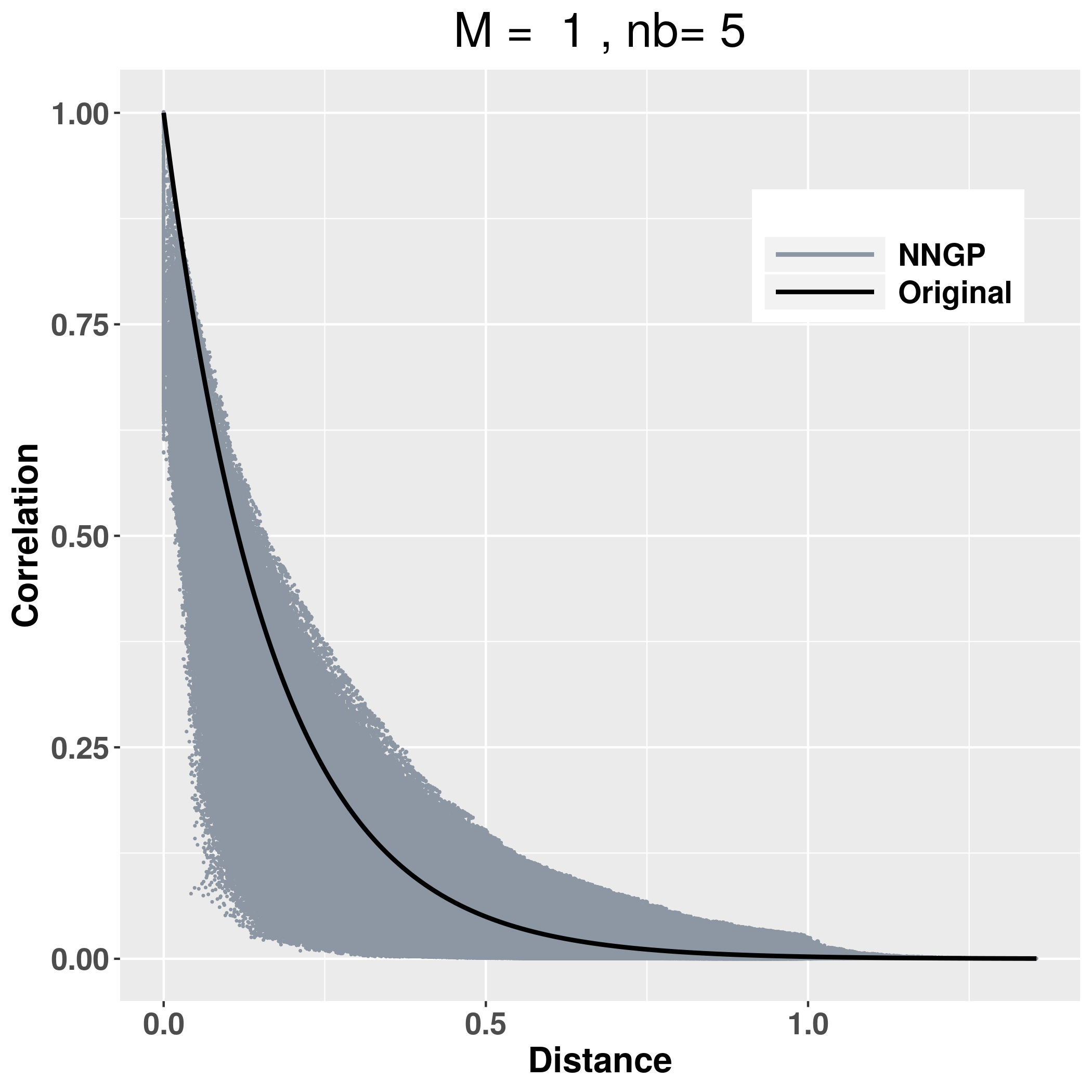
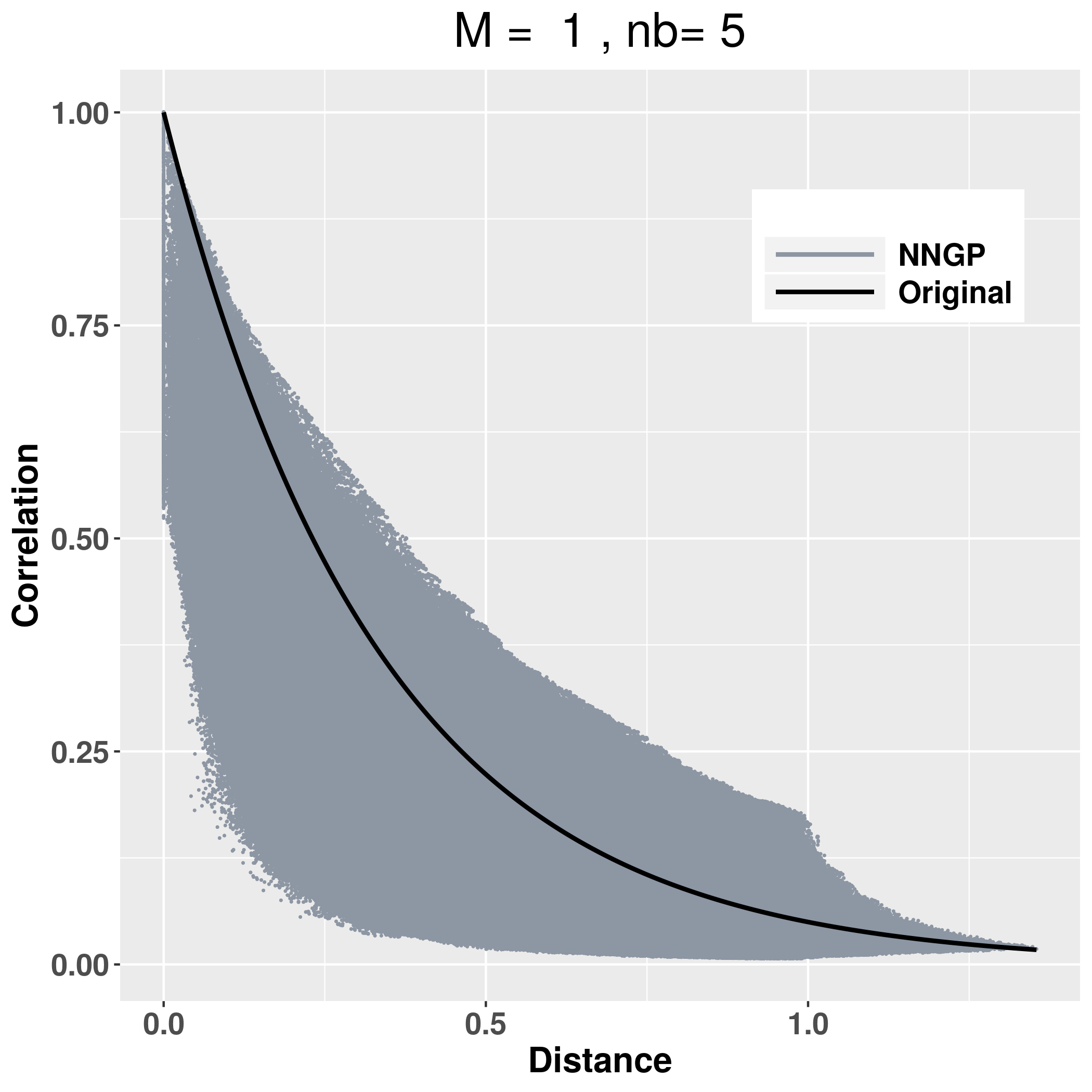
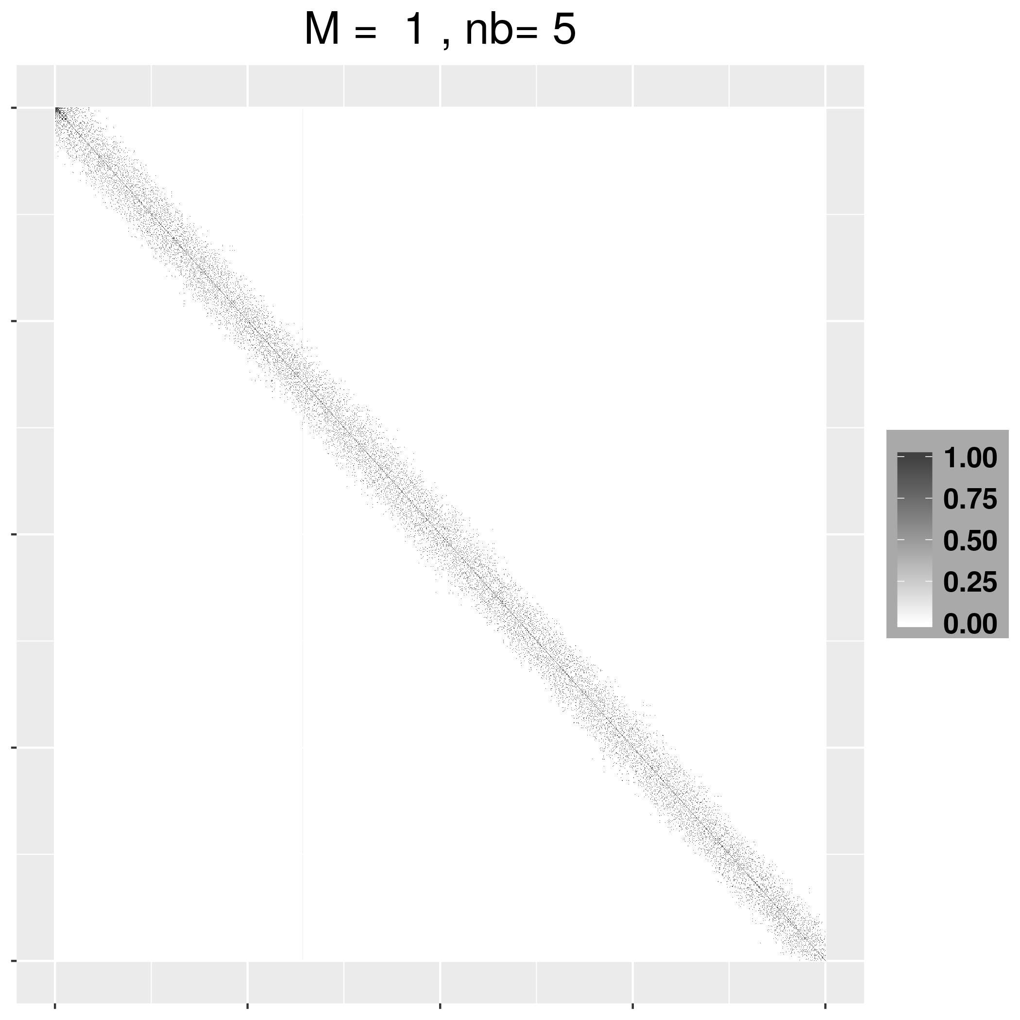
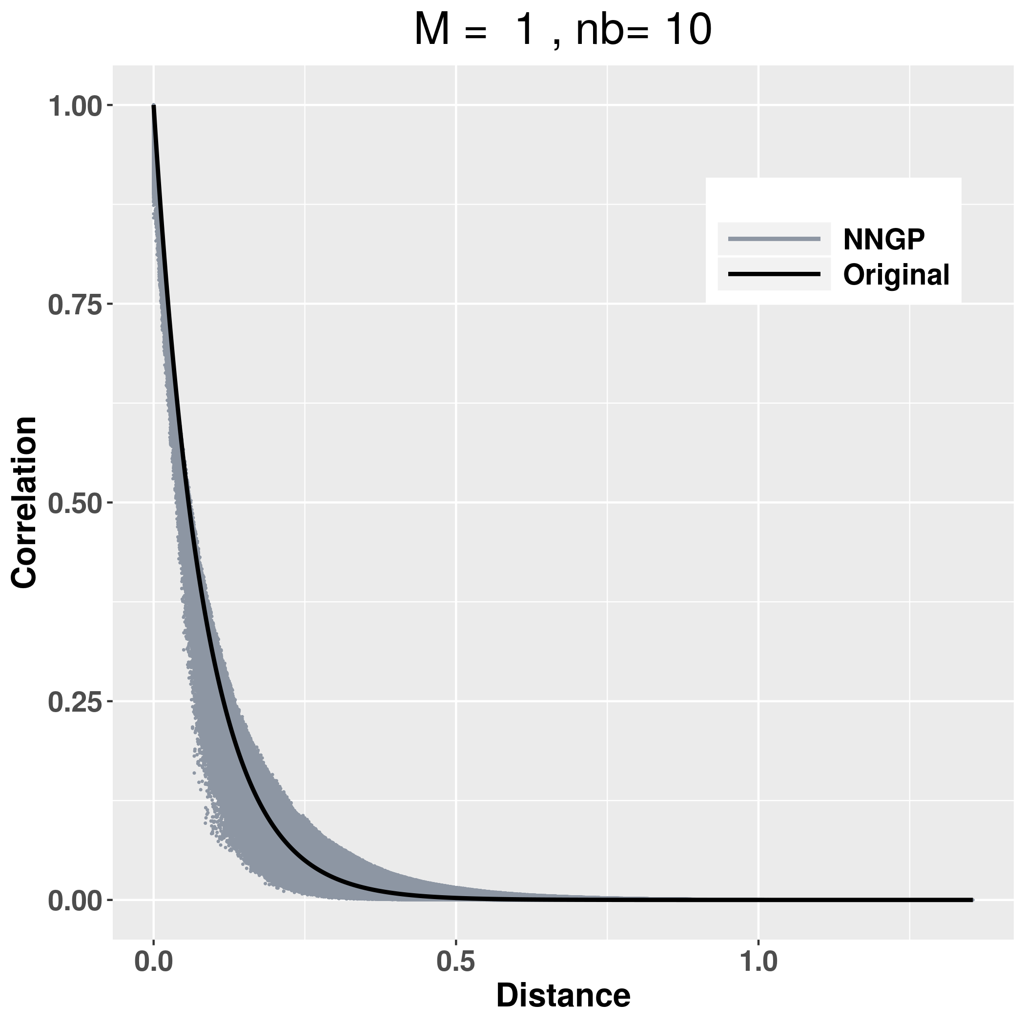
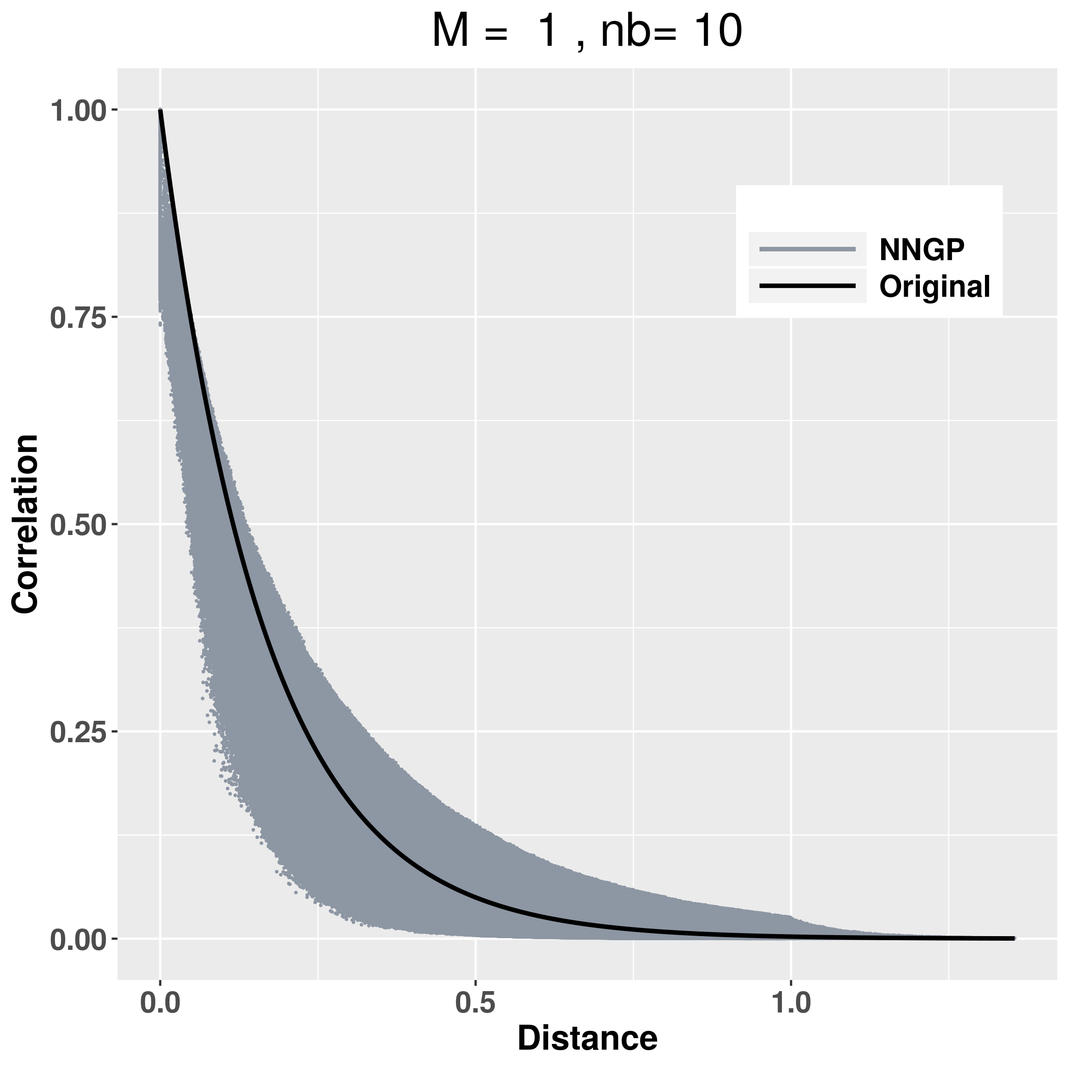
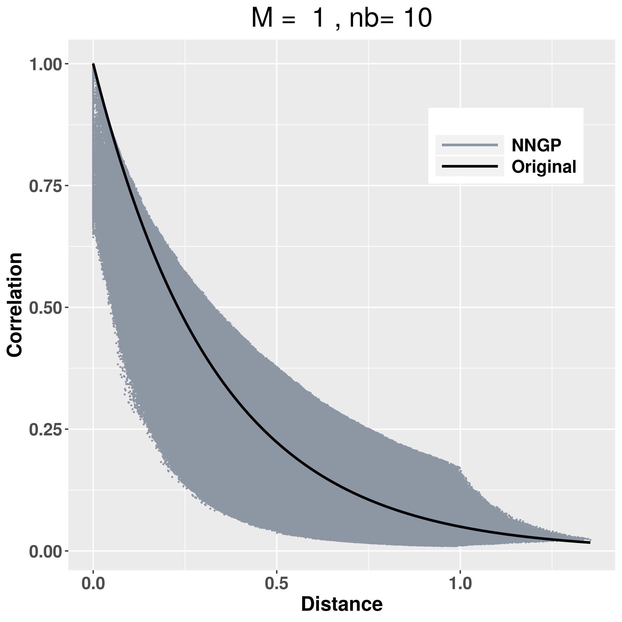
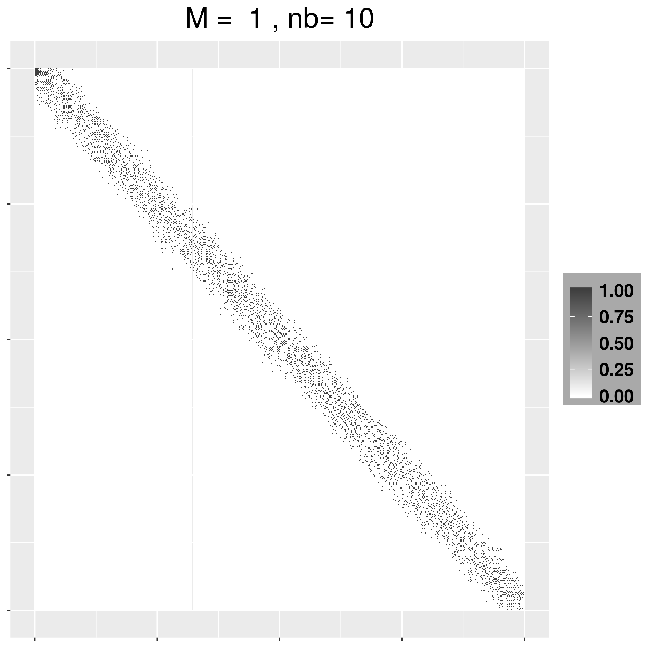
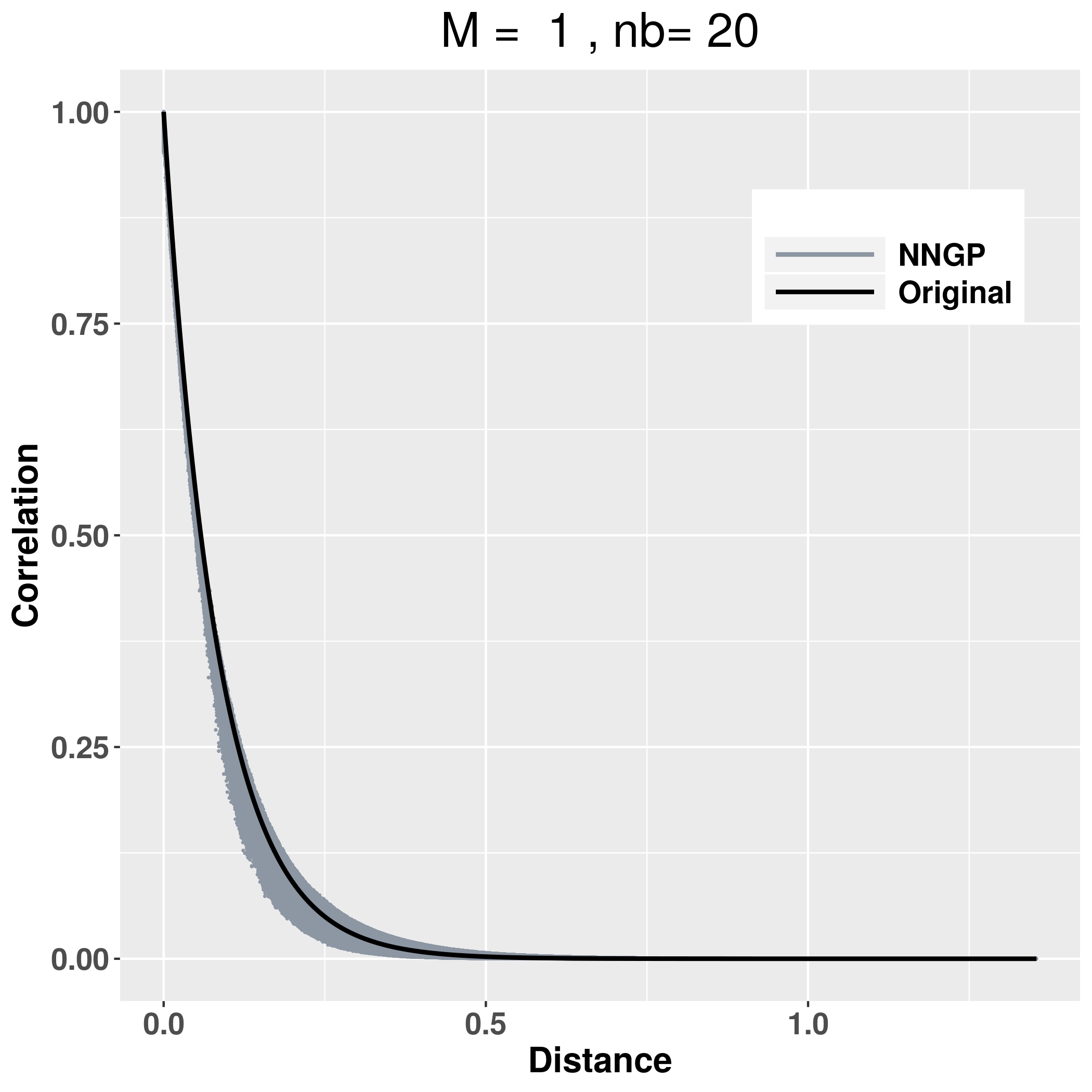
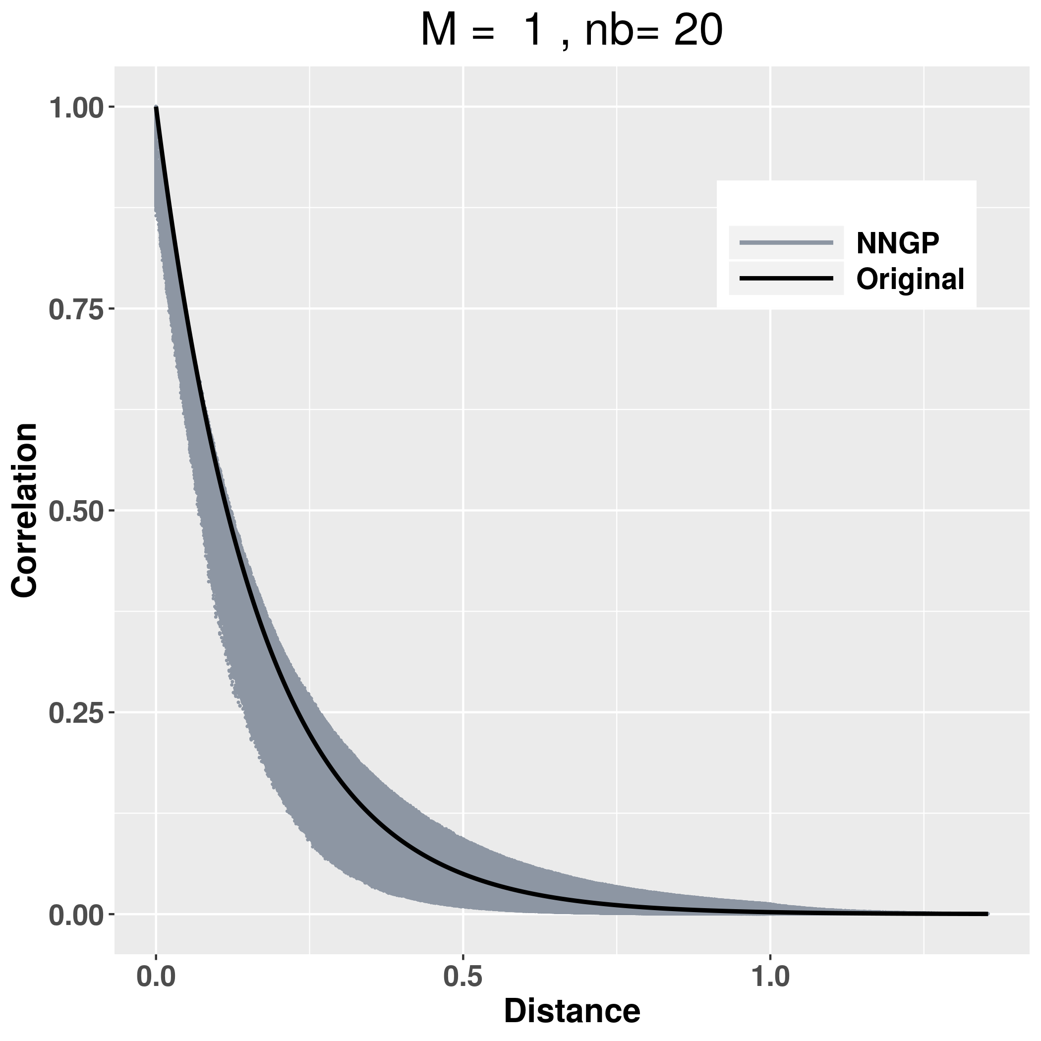
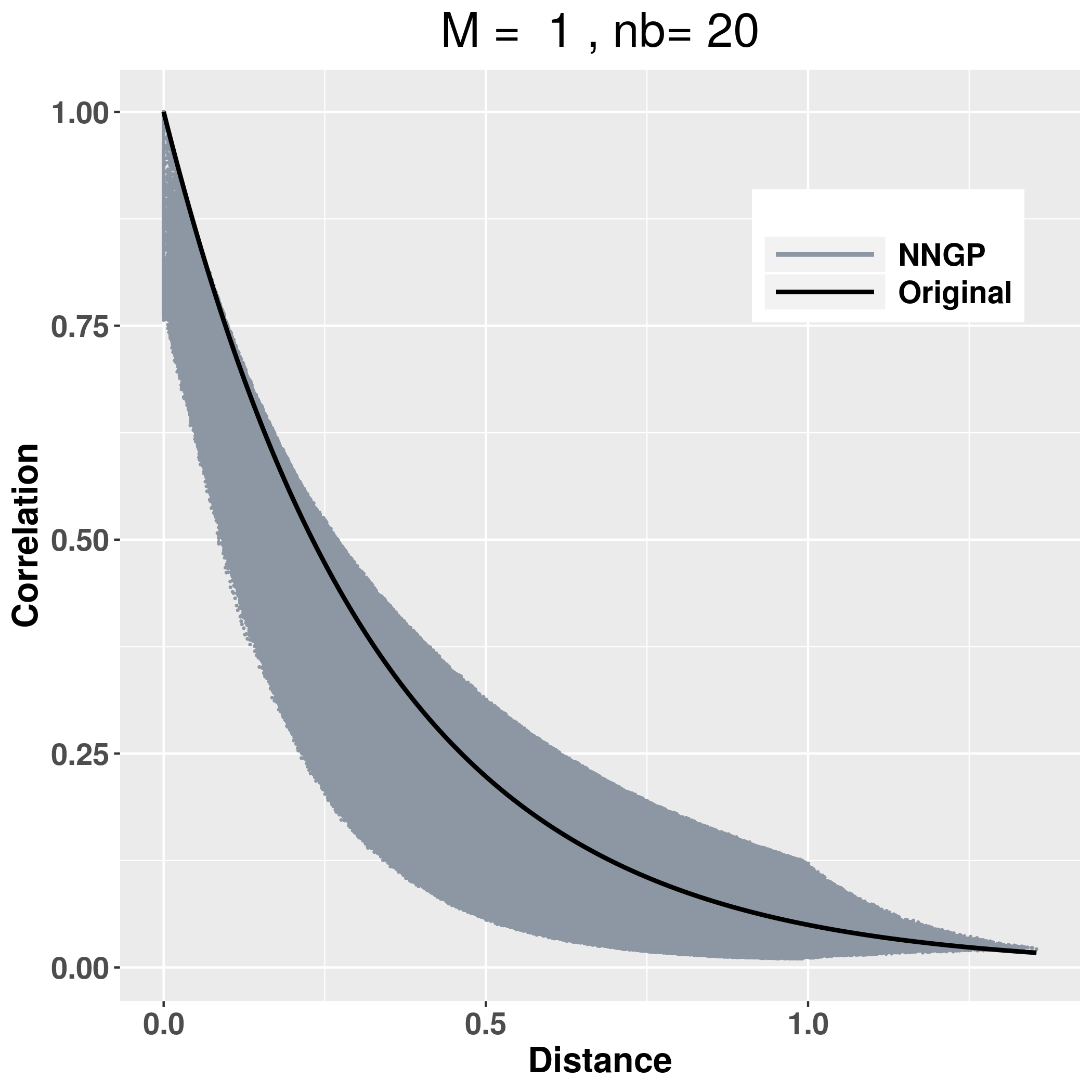
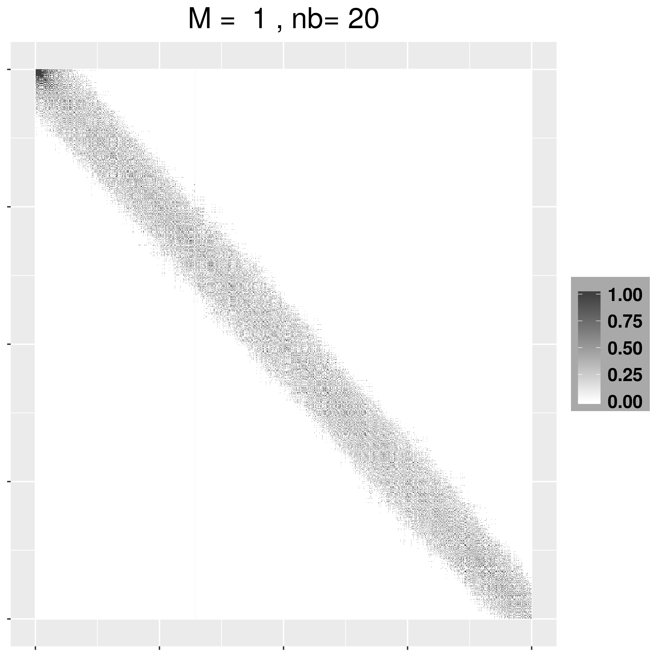
Figure 2: True exponential correlation of GP against distance (black lines) and empirical approximated correlations of NNGP aginst distance (blue dots) for: short range($\phi$ = 12, first column), medium range ($\phi$ = 6, second column) and large range ($\phi$ = 3, third column), and $nb=5$ neighbors (first row), $nb=10$ neighbors (second row) and $nb=20$ neighbors (third row). The fourth column presents Precision matrices for $nb=5$ neighbors (first row), $nb=10$ neighbors (second row) and $nb=20$ neighbors (third row), gray squares represent non-zero values.

$\phi=12$                          $\phi=6$                         $\phi=3$                         Q

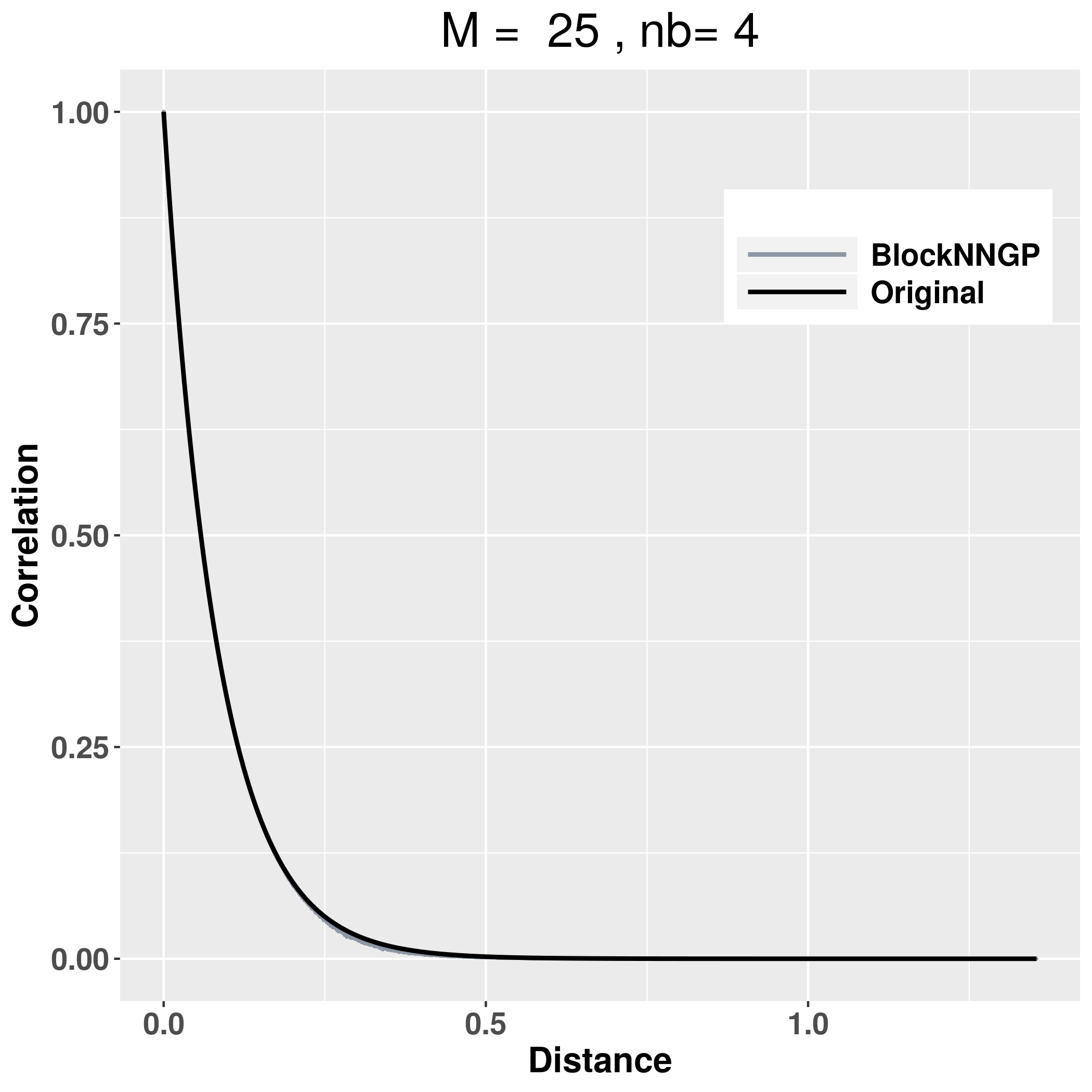
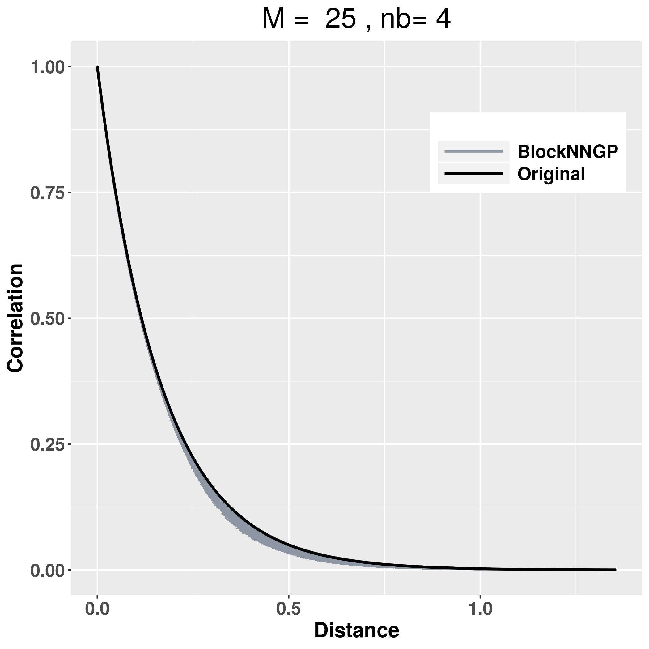
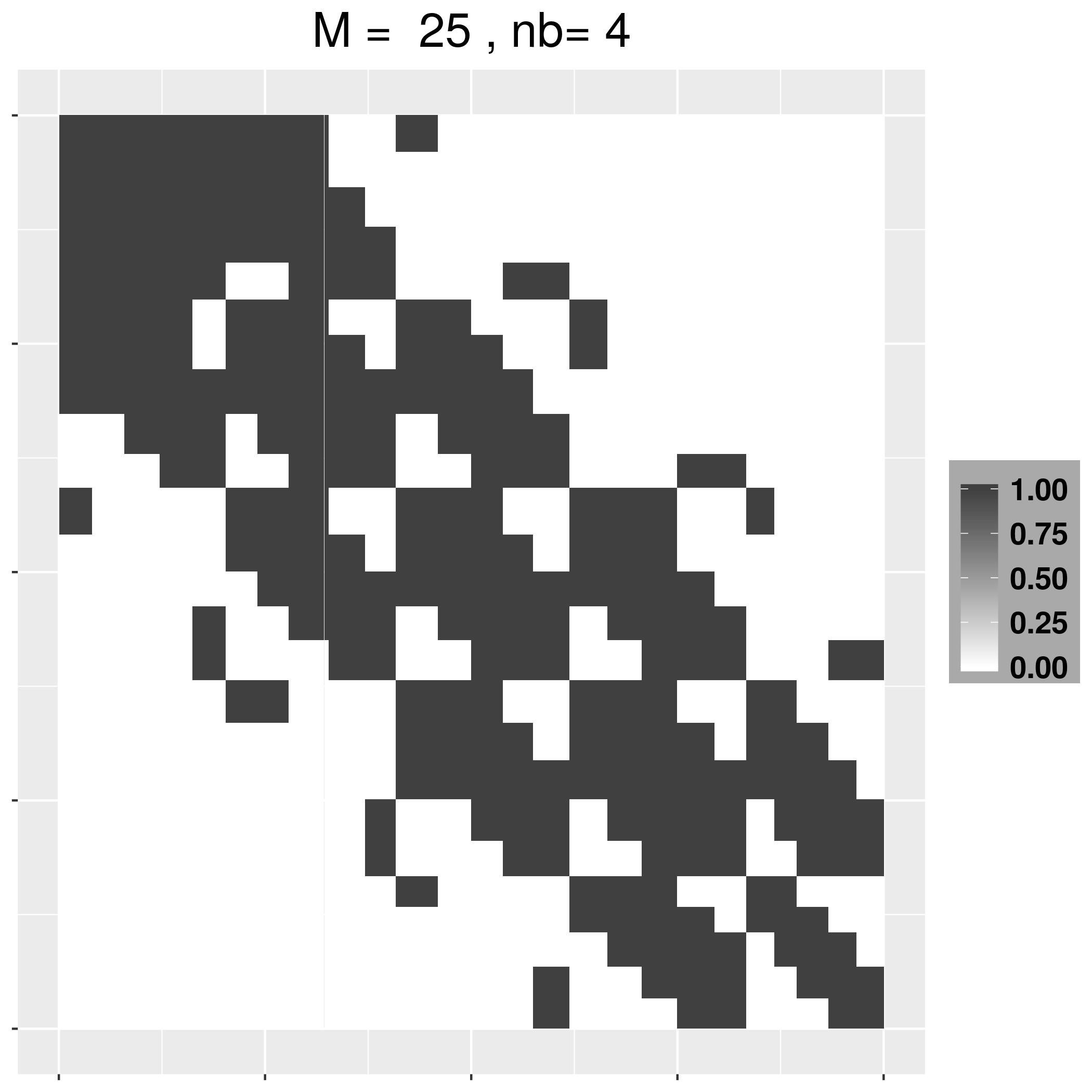
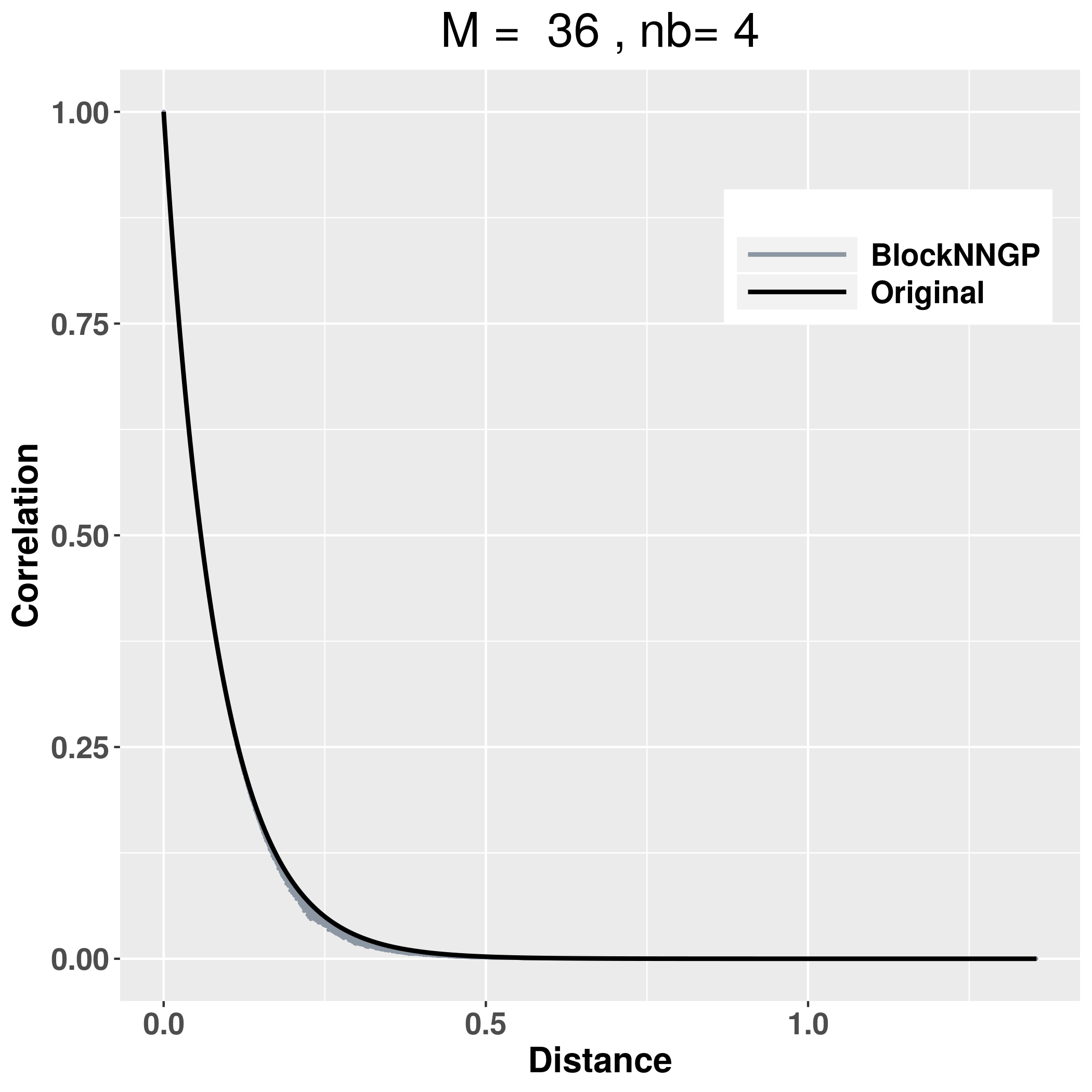
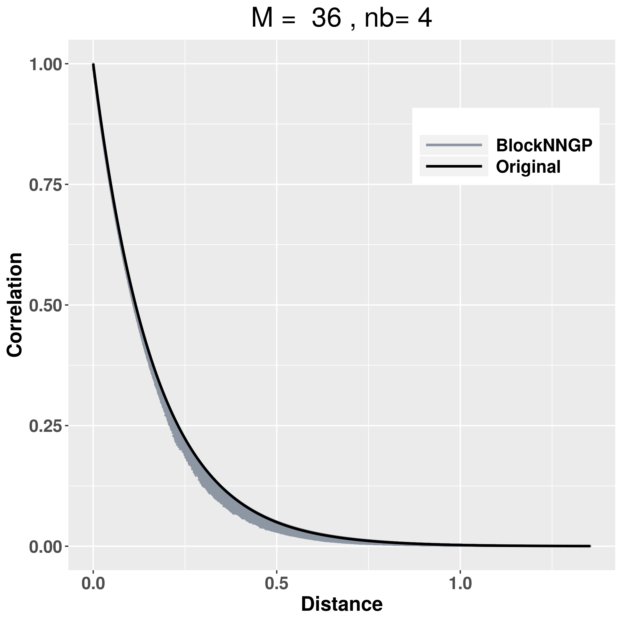
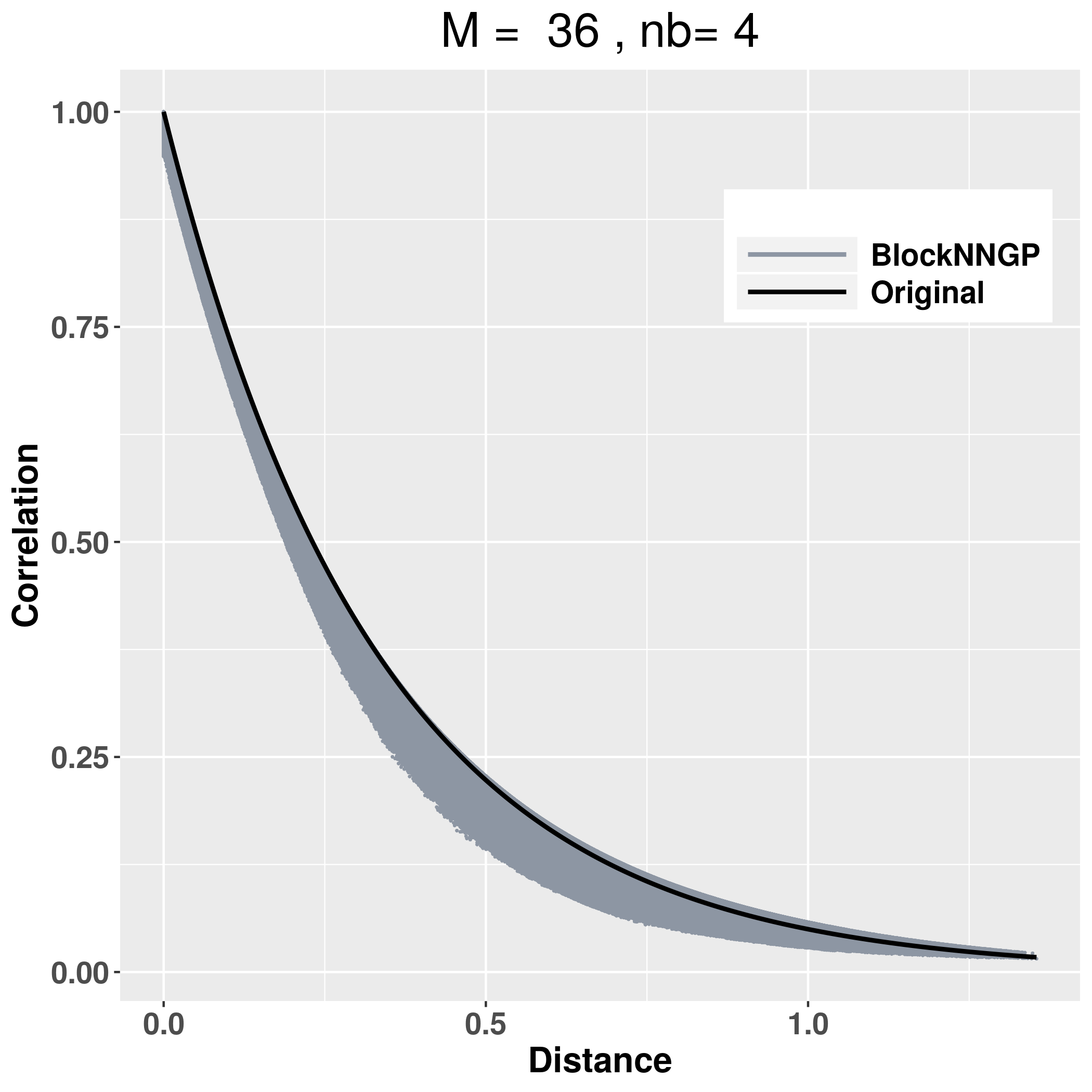
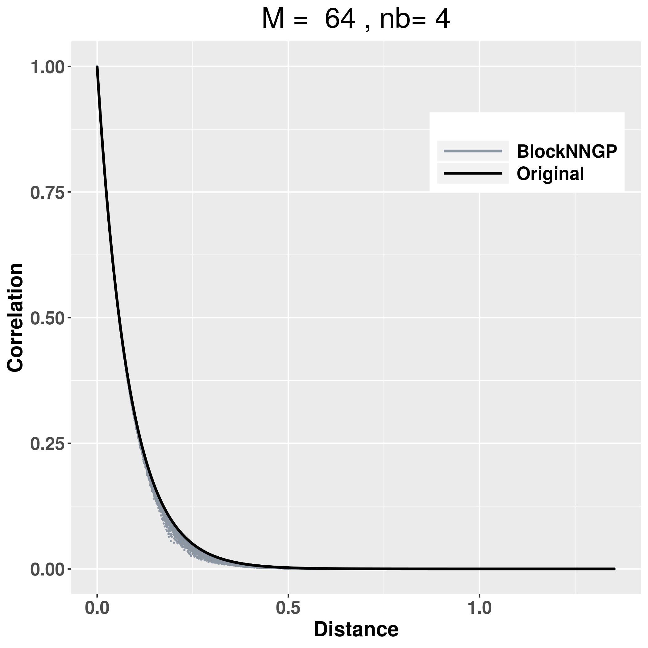
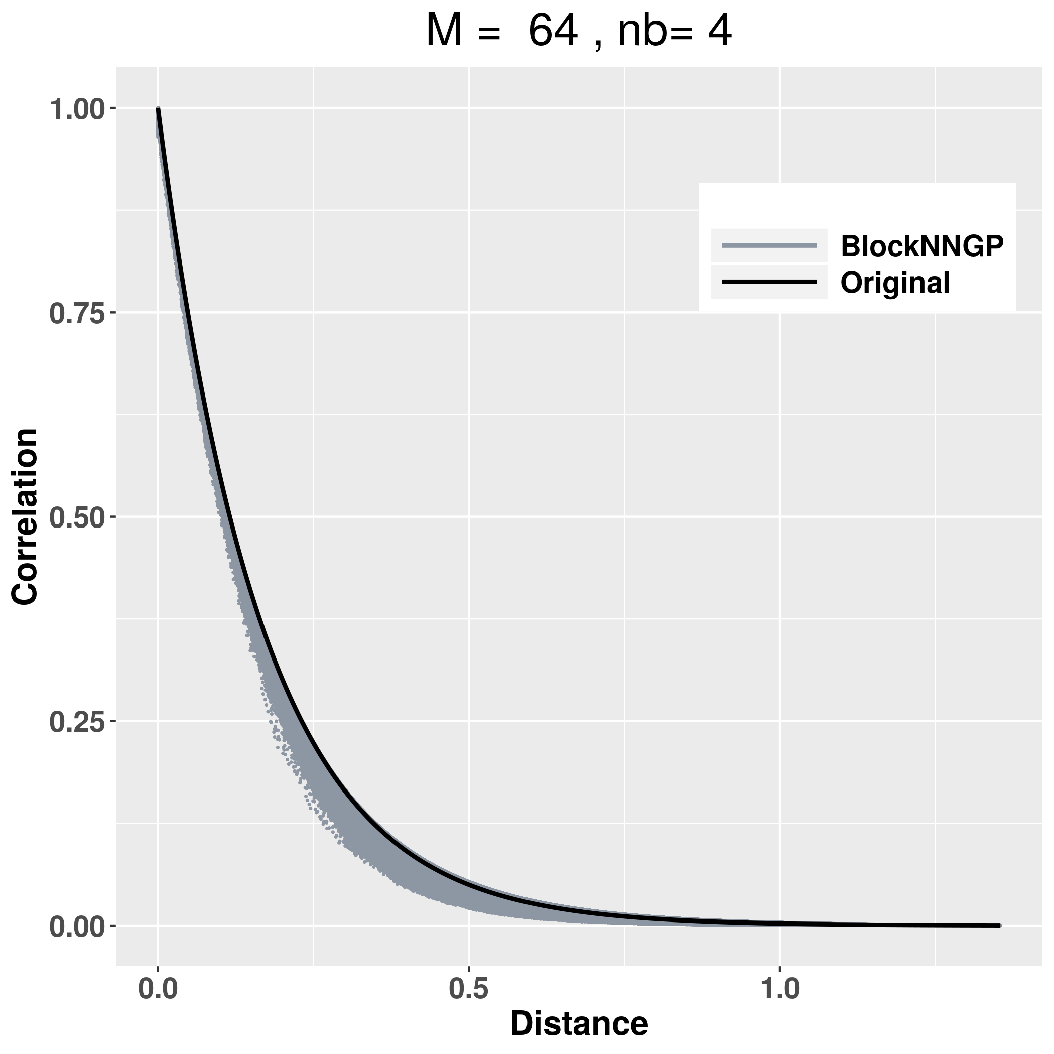
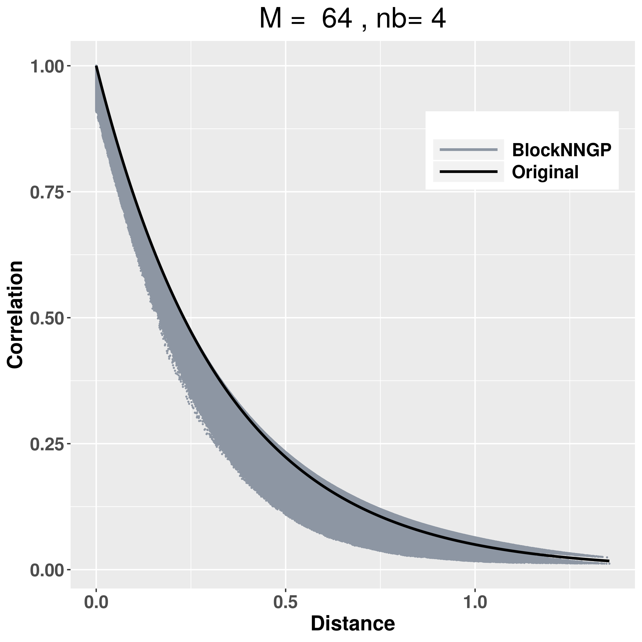
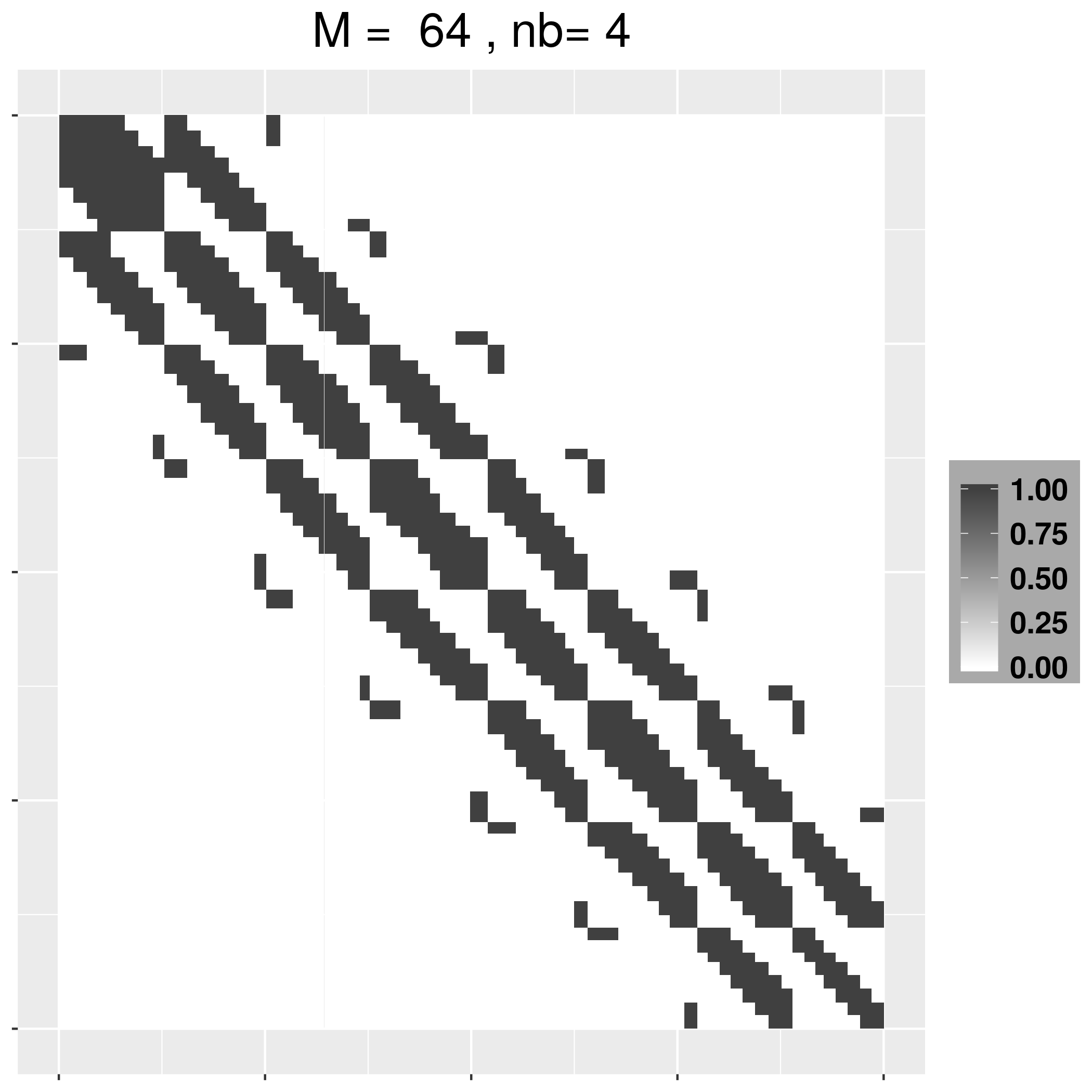
Figure 3: Regular blocks. True exponential correlation of GP against distance (black lines) and empirical approximated correlations of block-NNGP aginst distance (blue dots) for: short range($\phi$ = 12, first column), medium range ($\phi$ = 6, second column) and large range ($\phi$ = 3, third column), and $M=25$ blocks (first row), $M=36$ blocks (second row) and $M=64$ blocks (third row). The fourth column presents Precision matrices for $M=16$ blocks (first row), $M=36$ blocks (second row) and $M=64$ blocks (third row), gray squares represent non-zero values. In all cases, each block has $nb=4$ neighbor blocks.

Nevertheless, some cases show a discrepancy from the true correlations, specially, when the range is large or when the number of blocks is large. The block-NNGP precision matrix is a block sparse matrix, a more optimal structure in terms of computational gains. In practice there is a trade-off between accuracy of the block-NNGP approximation and the number of blocks used.

Another way to illustrate the difference between the NNGP, the block-NNGP and the exact GP is in terms of the Kullback-Leibler divergence (KLD). Figure 4 displays the square root of the KLD (SR-KLD) of the block-NNGP (upper) for different number of blocks ($M$) and number of neighbor blocks ($nb$), and the SR-KLD of the NNGP (lower panel) for different number of neighbors. We notice that for NNGP as the number of neighbors increases it clearly gives an improvement, nevertheless the loss of information is higher when the range is larger. While the block-NNGP with $nb=4$ clearly gives an improvement over $nb=2$, the results are quite similar for the three ranges, but the loss of information increases when the number of blocks becomes larger. In general, since the block-NNGP is expected to have more neighbors than NNGP it will, necessarily, provide a better approximation to the full process. For a formal proof we refer to Guinness, (2018); Banerjee, (2020).

$\phi=12$                                         $\phi=6$                                        $\phi=3$

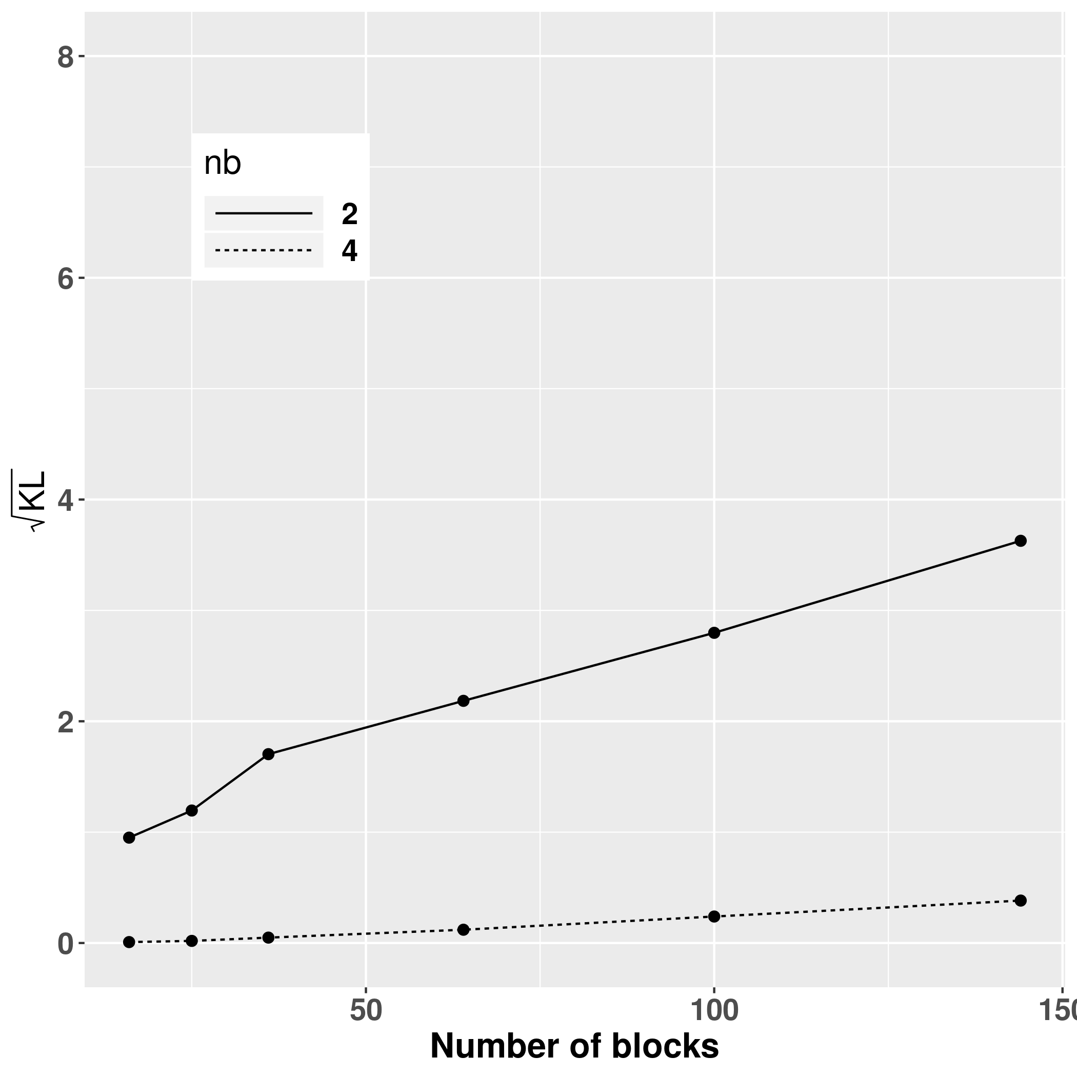
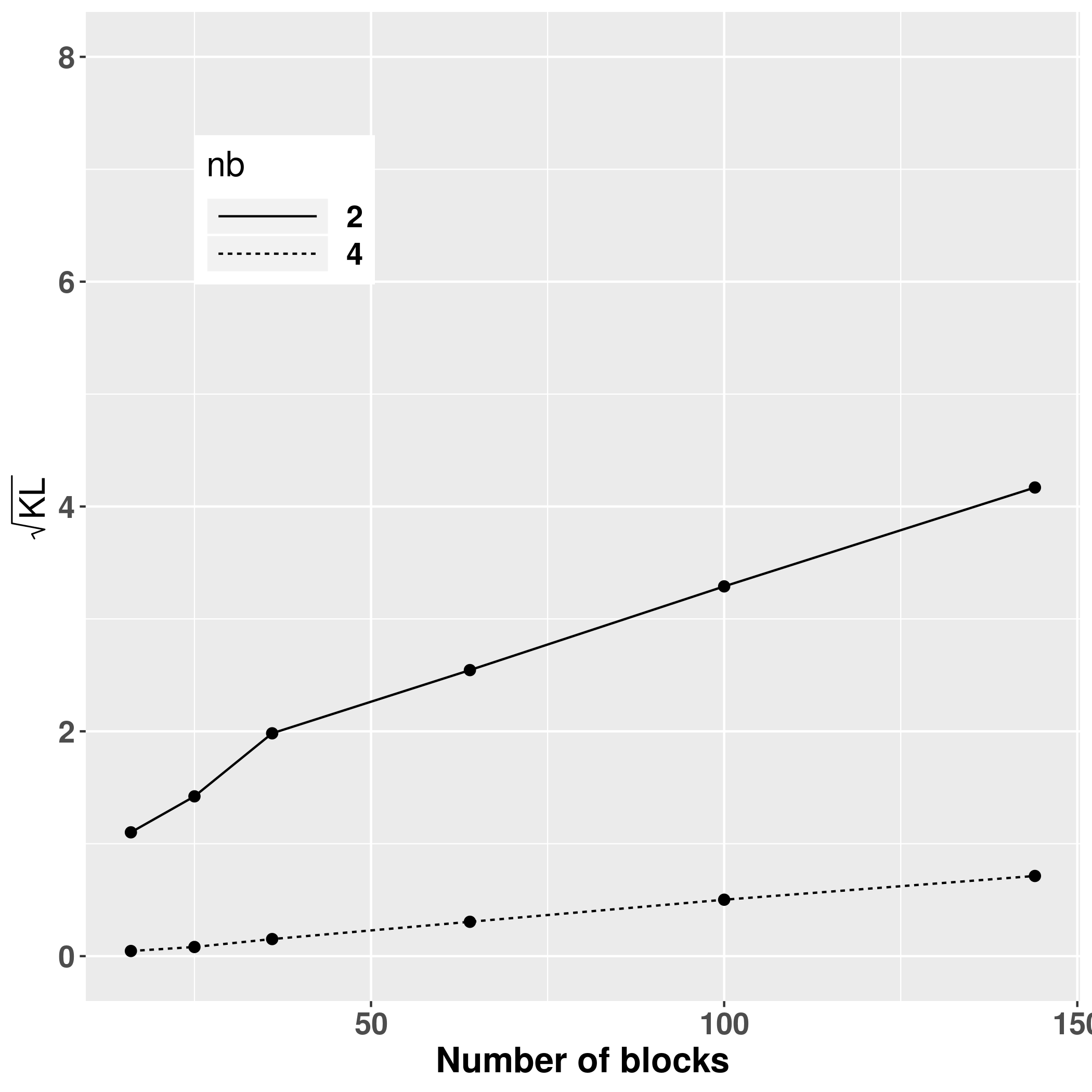
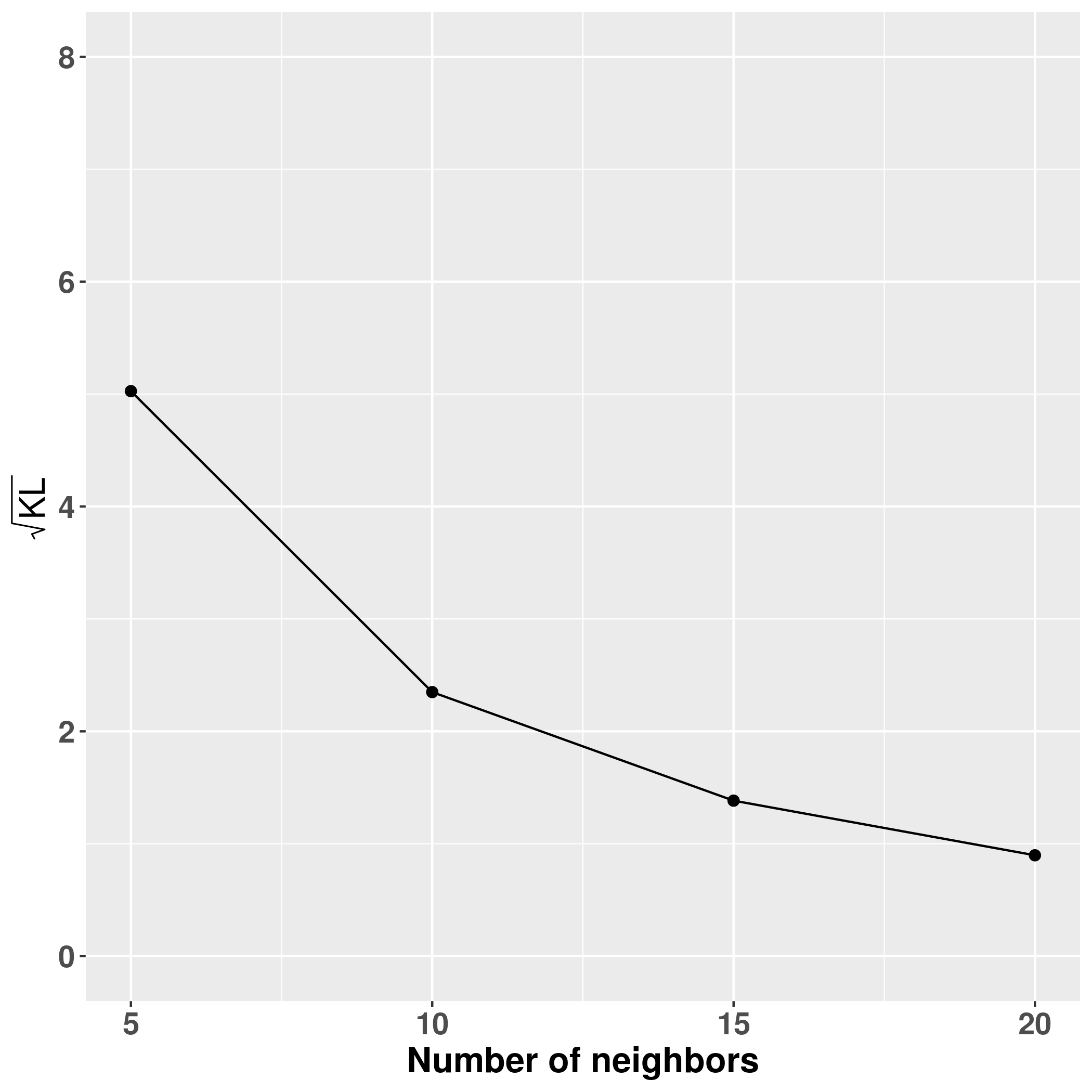
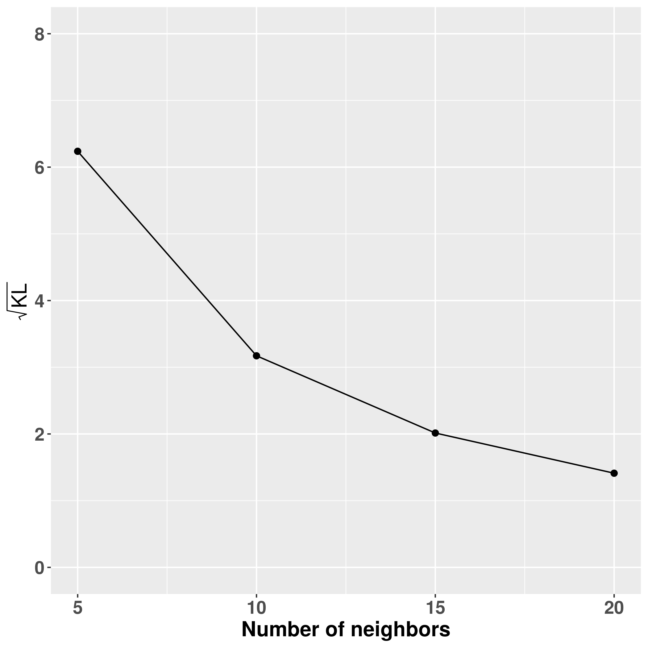
Figure 4: Upper panel: The square root of the Kullback-Leibler divergence of block-NNGP as a function of the number of blocks for 2000 locations and different ranges using the blockNNGP model with nb = 2 and nb = 4 neighbor blocks. Lower panel: The square root of the Kullback-Leibler divergence of NNGP as a function of the number of observations for 2000 locations and different ranges. First column: $\phi$ = 12 (short range), Second column: $\phi=6$ (medium range) and Third column: $\phi$ = 3 (large range).

2.1 Blocking strategies

The spatial domain ${\boldsymbol{D}}$ can be partitioned into several regions, either using a regular or an irregular block design (Eidsvik et al.,, 2014). In general, in order to achieve fast inference it is useful that each block has the same number of locations, otherwise for some blocks it will be expensive to perform matrices operations , instead of a balanced cost. With this in mind, the regular block design may not be practical. In practice, when the observed locations are almost uniformly distributed over the domain ${\boldsymbol{D}}$, it is recommended to use the regular block design. But when the observed locations are far from uniform, it is recommended to have more complicated partitioning schemes like irregular block design.

In particular, for the regular block design, the spatial domain is simply partitioned into $M$ non-intersecting rectangular subregions of approximately the same area. For the irregular block design, we propose to split the spatial domain into $M$ non-intersecting rectangular subregions with approximately the same number of points through a 2-dimensional (2-d) tree (Bentley,, 1975). Given a set of coordinates $s_{1},\dots,s_{n}$, the 2-d tree is constructed as follows: i) Compute the median ($Me$) of the coordinates, that is, at least 50% of the coordinates are equal or smaller than $Me$. ii) Then the spatial domain ${\boldsymbol{D}}$ is partitioned into rectangular regions ${\boldsymbol{D_{L}}}$ and ${\boldsymbol{D_{R}}}$, where ${\boldsymbol{D_{L}}}$ contains only the coordinates equal or smaller than $Me$. iii) Repeat i) and ii) recursively on both ${\boldsymbol{D_{L}}}$ and ${\boldsymbol{D_{R}}}$. iv) The recursion stops when the number of desired blocks $M$ is achieved. The last step was conditioned to fulfill our requirements.

To illustrate the process of our two blocking strategies, Figure 5 displays two examples. The first one shows the locations of $10000$ samples of joint frequency mining data in Norway, with a regular blocking, where $M=95$. And the second one shows the locations of $6000$ samples of precipitation in South America, with an irregular blocking, here $M=128$ and the approximated number of samples in each block is $47$.

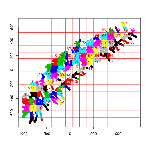
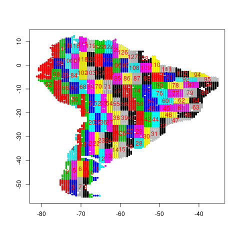
Figure 5: Left: Regular blocks for joint-frequency data, $n=10000$ locations. Right: Irregular blocks for Precipitation data, $n=6000$ locations.

2.2 Bayesian inference for block-NNGP models

Let $\bf{Y}=(Y(s_{1}),\dots,Y(s_{n}))^{T}$ be a realization of a spatial process defined for all $s_{i}\in{\boldsymbol{D}}\subset\Re^{2}$, $i=1,\dots,n$, where the random variable $Y_{i}=Y(s_{i})$ follows a generic distribution with pdf $\pi(y_{i}|\mu_{i},\theta_{0})$, which depends on the mean $\mu(s_{i})$ and some hyperparameters $\theta_{0}$. In a general geostatistical model the mean is linked to the linear predictor $\eta_{i}$ through a suitable link function $g(.)$ and the structure of the linear predictor has the next general form:

$$g(\mu(s_{i}))=\eta_{i}={\boldsymbol{X}}^{T}(s_{i}){\boldsymbol{\beta}}+w(s_{i})+\epsilon(s_{i}),$$ (7)

where ${\boldsymbol{\beta}}$ is a coefficient vector (or regression parameter), ${\boldsymbol{X}}^{T}(s_{i})$ is a vector of covariates, $w(s_{i})$ is a spatial structured random effect, thus ${\boldsymbol{w}}=(w(s_{1}),\dots,w(s_{n}))^{T}$ captures the spatial association, and $\epsilon(s_{i})\sim N(0,\tau^{2})$ models the measurement error. The usual Gaussian process prior for ${\boldsymbol{w}}\sim N(0,{\boldsymbol{C}}(\theta_{1}))$, where ${\boldsymbol{C}}(.)$ is some specific covariance function which depends on $\boldsymbol{\theta_{1}}=(\phi,\sigma^{2})$. Instead of this prior we assume that ${\boldsymbol{w}}\sim\mbox{block-NNGP}(0,{\boldsymbol{\widetilde{C}}})$. Further, we assign priors for ${\boldsymbol{\beta}}\sim N({\boldsymbol{\mu_{\beta}}},{\boldsymbol{\Sigma_{\beta}}})$ and for the parameters $\theta_{0},\phi,\sigma^{2},\tau^{2}$.

The model presented in (7) belongs to the latent Gaussian models (LGM) class. More specifically, we have that $Y_{i}$’s given the latent Gaussian process $\boldsymbol{x}$=$\{{\boldsymbol{\beta}},{\boldsymbol{w}}\}$ and possible hyperparameters $\boldsymbol{\theta}=(\theta_{0},\sigma^{2},\phi,\tau^{2})$, are assumed conditionally independent. Hence, the posterior estimates of parameters are computed using INLA.

With regard to the distribution of the latent process, since ${\boldsymbol{w}}\sim\mbox{block-NNGP}(0,{\boldsymbol{\widetilde{Q}^{-1}}})$, therefore the latent process $\boldsymbol{x}\sim N(0,{\boldsymbol{Q}})$, where

$$\boldsymbol{Q}=\left[\begin{array}[]{cc}\boldsymbol{\widetilde{Q}}&\boldsymbol{0}\\ \mathbf{0}&\boldsymbol{Q}_{\beta}\end{array}\right]$$

is sparse, and it can improve computational performance dramatically. We also remark that the structure of this precision matrix is particularly ideal, because $\boldsymbol{\widetilde{Q}}$ is built from blocks (see proposition 2 and (6)) and INLA can exploit fast parallel computation algorithms for blocks. Moreover the whole algorithm does not need to store $n\times n$ dense distance matrices to compute $\boldsymbol{\widetilde{Q}}$, it only stores ${\boldsymbol{M}}$ small dense matrices.

Then the joint posterior distribution of the LGM can be computed using the likelihood distribution of $\boldsymbol{Y}$, the distribution of the latent Gaussian field $\boldsymbol{x}$ and the distribution of hyperparameters $\boldsymbol{\theta}$ as

$$\pi(\boldsymbol{x},\boldsymbol{\theta}|\boldsymbol{y})\propto\pi(\boldsymbol{\theta})|\boldsymbol{Q}|^{1/2}\exp\left[-\frac{1}{2}x^{\top}Qx+\sum_{i=1}^{n}\log\{\pi(y_{i}|\boldsymbol{x},\boldsymbol{\theta})\}\right],$$

where the determinant of ${\boldsymbol{Q}}$ is easily computed from the Cholesky decomposition of $\boldsymbol{\widetilde{Q}}$ which inherits the sparsity property of $\boldsymbol{\widetilde{Q}_{S}}$ in Proposition 2.

The posterior marginals of the latent variables $\pi(x_{i}|y)$ and the posterior marginal of hyperparameters $\pi(\theta_{s}|y)$ are defined by

$$\pi(x_{i}|y)=\int\pi(x_{i}|\theta,y)\pi(\theta|y)d\theta\mbox{ and }\pi(\theta_{j}|y)=\int\pi(\theta|y)d\theta_{-j},$$

where $i=1,\ldots,n$. INLA provides approximations for the posterior marginals of the latent variables and hyperparameters, as given by

$$\widetilde{\pi}(x_{i}|y)=\int\widetilde{\pi}(x_{i}|\theta,y)\widetilde{\pi}(\theta|y)d\theta\mbox{ and }\widetilde{\pi}(\theta_{j}|y)=\int\widetilde{\pi}(\theta|y)d\theta_{-j},$$ (8)

which are both very accurate and extremely fast to compute. Here, $\widetilde{\pi}$ denotes an approximation to a pdf. In summary, the main idea of INLA is divided into the following tasks: First, it provides a Gaussian approximation of $\widetilde{\pi}(\theta|y)$ to the joint posterior of hyperparameters given the data $\pi(\theta|y)$. Then, it provides an approximation of $\widetilde{\pi}(x_{i}|\theta,y)$ for the marginals of the conditional distribution of the latent field given the data and the hyperparameters $\pi(x_{i}|\theta,y)$. And finally, it explores $\widetilde{\pi}(\theta|y)$ on a grid and uses it to integrate out $\theta$ and $\theta_{-j}$ in (8). For more details on INLA calculations, we refer to Rue et al., (2009).

Following Finley et al., (2019), spatial prediction can be carried out after parameter inference. Conditioning on a particular estimated value of the parameters $({\boldsymbol{\theta}},{\boldsymbol{\beta}})$, spatial prediction amounts to finding the posterior predictive distribution on a set of prediction locations $u_{i}$, that is, $\pi(y(u_{i})|{\boldsymbol{y}})$. Without loss of generality, if we consider all observed data for estimation, thus ${\boldsymbol{S}}$ comprises the observed locations, while the new location points for predictions belong to the finite set ${\boldsymbol{U}}$. Furthermore, since the components of ${\boldsymbol{w_{U}}}|{\boldsymbol{w_{S}}}$ are independent, we can update $w(u_{i})$ for each $i=1,\dots,l$, from $\pi(w(u_{i})|{\boldsymbol{w_{S}}},{\boldsymbol{\beta}},{\boldsymbol{\theta}},{\boldsymbol{y}})\sim N(m,v)$, where $m={\boldsymbol{C}}^{T}_{u_{i},{\boldsymbol{N(u_{i})}}}{\boldsymbol{C}}^{-1}_{{\boldsymbol{N(u_{i}),N(u_{i})}}}{\boldsymbol{w(N(s_{0}))}}$ and $v=\sigma^{2}-{\boldsymbol{C}}^{T}_{u_{i},{\boldsymbol{N(u_{i})}}}{\boldsymbol{C}}^{-1}_{{\boldsymbol{N(u_{i}),N(u_{i})}}}{\boldsymbol{C}}_{u_{i},{\boldsymbol{N(u_{i})}}}$. Therefore, the block-NNGP is especially useful here because the posterior sampling for ${\boldsymbol{w_{U}}}$ is cheap, given that their components are independent, each $w(u_{i})$ is only based on the observations that lie in the block that it belongs. Now using the posterior samples of $w(u_{i})$, the posterior predictive sampling is performed through $y(u_{i})|{\boldsymbol{w_{U}}},{\boldsymbol{w_{S}}},{\boldsymbol{\beta}},{\boldsymbol{\theta}},{\boldsymbol{y}}\sim N(X^{T}(u_{i}){\boldsymbol{\beta}}+w(u_{i}),\tau^{2})$.

In the supplementary material B we present in details a full-MCMC approach using a collapsed MCMC strategy. This strategy was shown to improve convergence and reduce running times in comparison to other MCMC strategies (Finley et al.,, 2019). It is also important to emphasize that INLA avoids the complex updating schemes, long running times, and diagnostic convergence checks of MCMC, and uses directly the sparse precision matrix of the block-NNGP which is also computed using fast parallel algorithms for blocks and Cholesky decomposition. For this reason we focus our results and discussions mainly using INLA.

3 Simulation results

In order to assess the performance of the block-NNGP models, we present the next simulation experiments. We generate $s_{i}$ sites on a spatial domain $[0,1]\times[0,1]$ where $i=1,\dots,2500$ and the random spatial effects $w(s_{i})$, under a zero mean Gaussian process model ${\boldsymbol{w}}\sim GP(0,{\boldsymbol{C}}(\phi,\sigma^{2}))$, where ${\boldsymbol{C}}(.)$ is an exponential covariance function with elements $C(s_{i},s_{j})=\sigma^{2}\exp(-\phi\|s_{i}-s_{j}\|)$. We set $\sigma^{2}=1$ and the effective range ($r$) is studied for a variety of settings chosen to mimic the range of behaviour we might observe in practice: (i) SIM I: $r$ = 0.16 ($\phi$ = 12); (ii) SIM II: $r$ = 0.33 ($\phi$ = 6); (iii) SIM III: $r$ = 0.67 ($\phi$ = 3), which represent small, medium and large effective ranges, respectively. We also generate the covariates $x_{i}\sim N(0,1)$, then ${\boldsymbol{X}}(s_{i})=(1,x_{i})^{T}$. The values of the regression parameters are given by ${\boldsymbol{\beta}}=(1,5)^{T}$ and the value of the nugget effect is $\tau^{2}=0.1$. Finally we draw $n=2500$ samples from $Y(s_{i})\mid\beta,\phi,\sigma^{2},\tau^{2}\sim N({\boldsymbol{X}}^{T}(s_{i}){\boldsymbol{\beta}}+w(s_{i}),\tau^{2}).$ We let ${\boldsymbol{S}}$ be a set of $2000$ locations and ${\boldsymbol{U}}$ be the set of the remaining observations used to assess predictive performance.

First we implemented the full-MCMC (see supplementary material B) for full Gaussian process (full GP), NNGP models ($nb=10$ and $nb=20$), a few regular (R) block-NNGP models and irregular (I) block-NNGP models, under scenario SIM I. We used flat prior distributions for $\beta$, for the spatial decay $\phi$ we assigned a uniform prior $U(1,30)$, which is equivalent to a range between approximately 0.067 and 2 units, and for $\sigma^{2}$ w and $\tau^{2}$ we assigned inverse gamma priors $IG(2,1)$. Posterior inference was based upon three chains of 25000 iterations (with a burn-in of 5000 iterations). The results are are shown in Table 1. The parameter estimates were quite accurate but very expensive; in the best scenario the running time for a block-NNGP model was about 17000 seconds, showing that the computational time using MCMC is too long. We also point out that the computational cost for block-NNGP models was the lower one.

Table 1: SIM I ($\phi$ = 12). Full MCMC results. Summary of mean posterior parameter estimates and parameter posterior summary credible intervals (2.5, 97.5).

		Full-GP	NNGP	NNGP	(R)M=64	(R)M=100	(I)M=64	(I)M=128
	True		nb=10	nb=20	nb=2	nb=1	nb=1	nb=2
$\beta_{0}$	1	0.92	1.03	1.07	1.05	1.05	1.1	1.13
		(0.4,1.31)	(0.69,1.46)	(0.65, 1.39)	(0.72,1.33)	(0.85,1.3)	(0.89, 1.34)	(0.82,1.37)
$\beta_{1}$	5	5.02	5.02	5.02	5.02	5.02	5.02	5.02
		(5, 5.05)	(5,5.04)	(5,5.05)	(5,5.05)	(5,5.05)	(5,5.04)	(5, 5.04)
$\sigma^{2}$	1	1.09	1.08	1.06	1.02	1.06	1.01	1.03
		(0.85,1.54)	(0.86,1.52)	(0.84,1.54)	(0.82,1.42)	(0.87,1.32)	(0.83,1.32)	(0.84,1.34)
$\phi$	12	11.08	11.23	11.5	12.15	11.62	12.16	11.38
		(7.28, 14.8)	(7.77,14.75)	(7.48,15.24)	(8.31,15.62)	(8.74,14.54)	(8.83,15.2)	(0.08,0.12)
$\tau^{2}$	0.1	0.1	0.1	0.1	0.1	0.1	0.1	0.1
		(0.08, 0.12)	(0.08,0.12)	(0.08,0.12)	(0.08,0.12)	(0.09,0.12 )	(0.08,0.12)	(8.49,14.5)
Time (sec)		21620.86	19514.39	22775.03	22738.14	16122.3	17067.59	17583.05

We were able to fit all the next models throughout INLA: (i) NNGP models ($nb=5,10,15,20,30,50$), (ii) regular (R) block-NNGP models and (iii) irregular (I) block-NNGP models, under all the scenarios proposed, in few minutes or seconds. For the block-NNGP models we test different number of blocks and neighbor blocks to investigate how different blocking schemes influence the estimation and prediction capabilities. The number of regular blocks are $M=9,16,25,36,49,81,100.$ The number of irregular blocks are $M=8,16,32,64,128.$ Moreover, the number of neighbor blocks are $nb=2,4,6$. We use similar priors as in the full-MCMC, but for $\tau^{2}$ we assigned gamma priors $G(1,5\times 10^{-05})$. Our implementation in R-INLA (w.r-inla.org ) and subsequent analysis were run on a Linux workstation with 32 GB of RAM and Intel quad-Xeon processor with 12 cores.

The criteria assessment and time requirements for scenarios SIM I ($\phi=12$) and SIM II ($\phi=6$) are reported in the supplementary material C. The results obtained confirm that the NNGP and block-NNGP models show a very good performance when the range is not too large. Here we present the results for the scenario SIM III, corresponding to a process that has a large effective range. Figure 6 shows the running time, LPML and WAIC for block-NNGP models using regular or irregular blocks and NNGP models. We observe that the running time for all the block-NNGP models is fast, even for block-NNGP models with a high number of neighbors, for instance using $\geq 36$ blocks, it takes less than $800$ seconds. We also remark a slightly time reduction for block-NNGP models with irregular blocks. In particular, the time requirements decreases when the number of blocks $M$ increases or the number of neighbor $nb$ decreases. Computing times requirements for the NNGP are lower due to the lower number of neighbors, but the running time for NNGP models increases as the number of neighbor increases too.

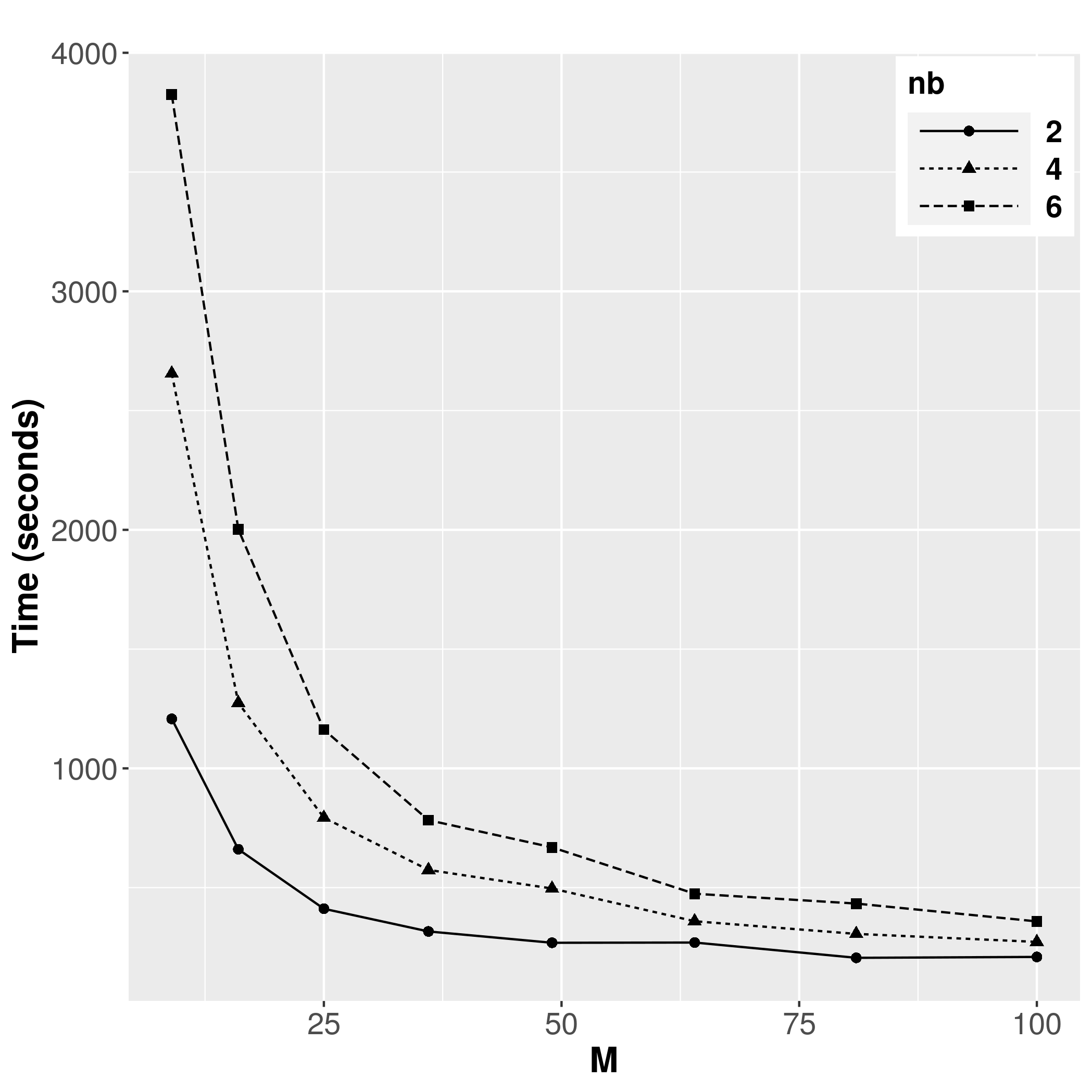
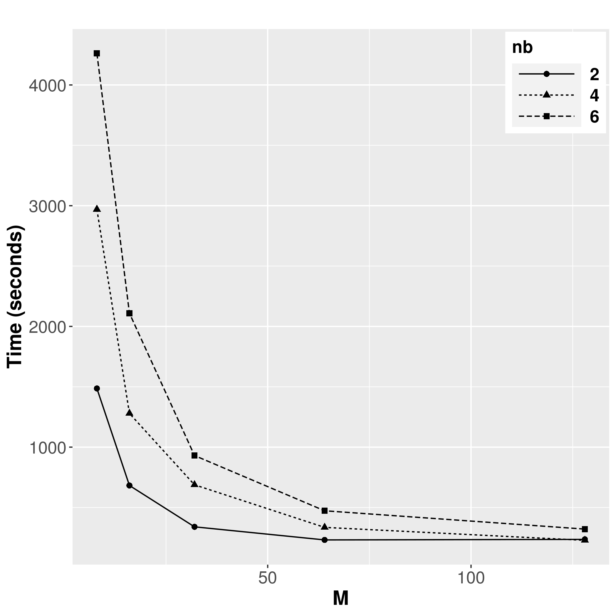
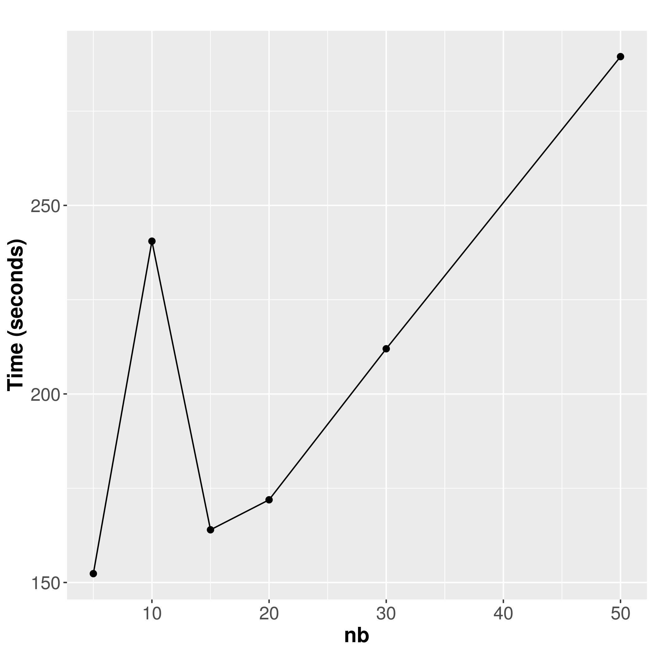
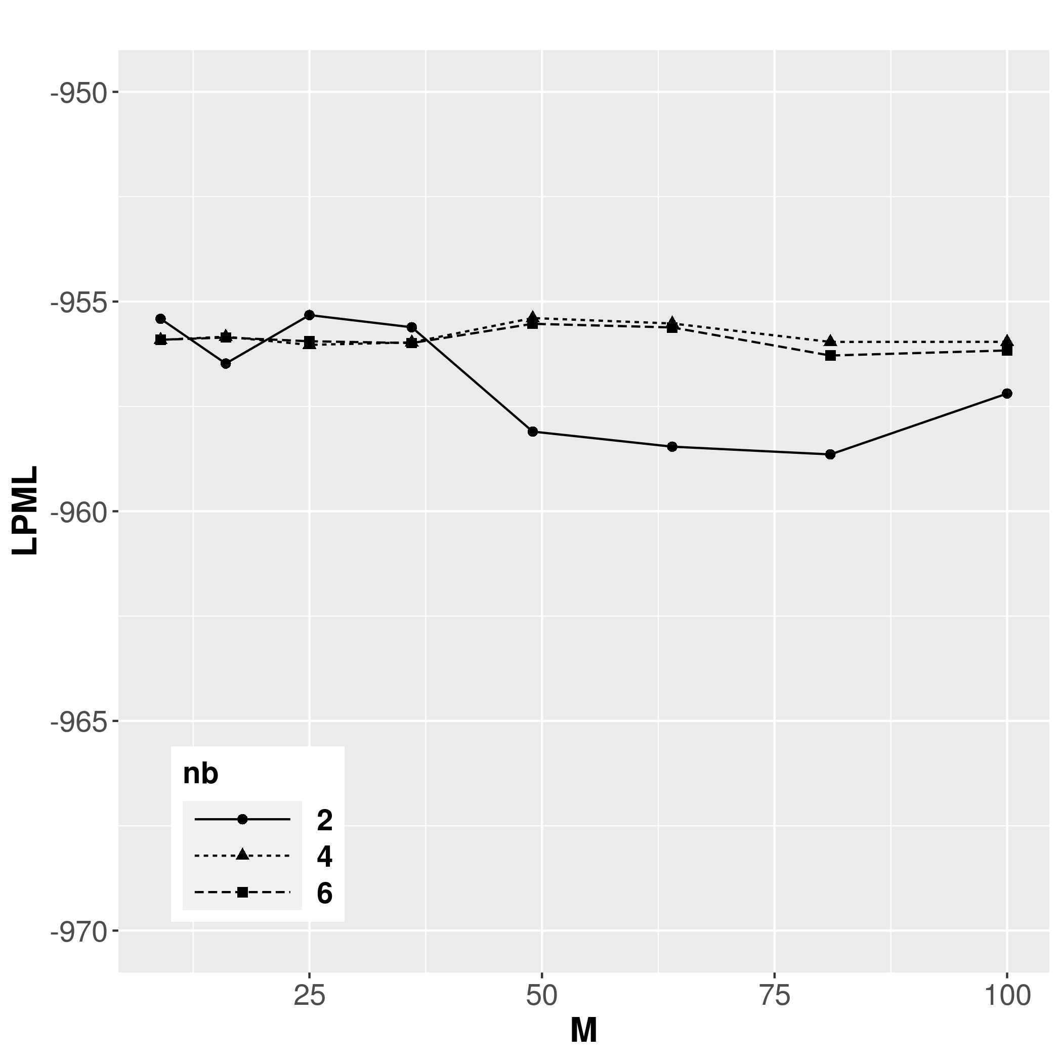
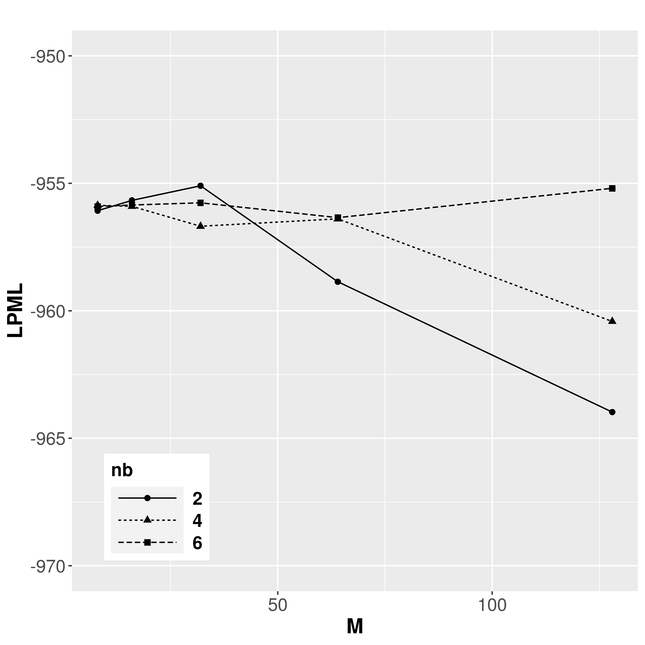
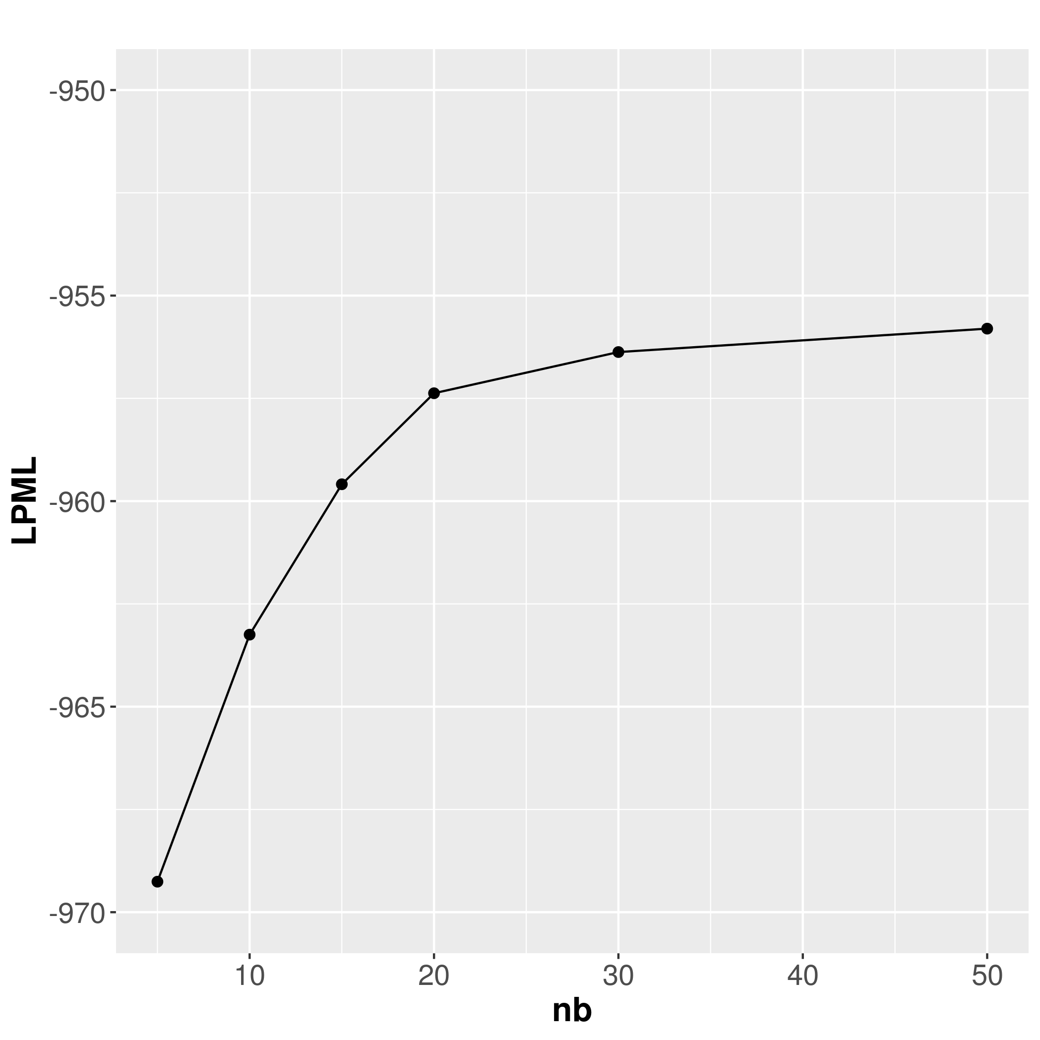
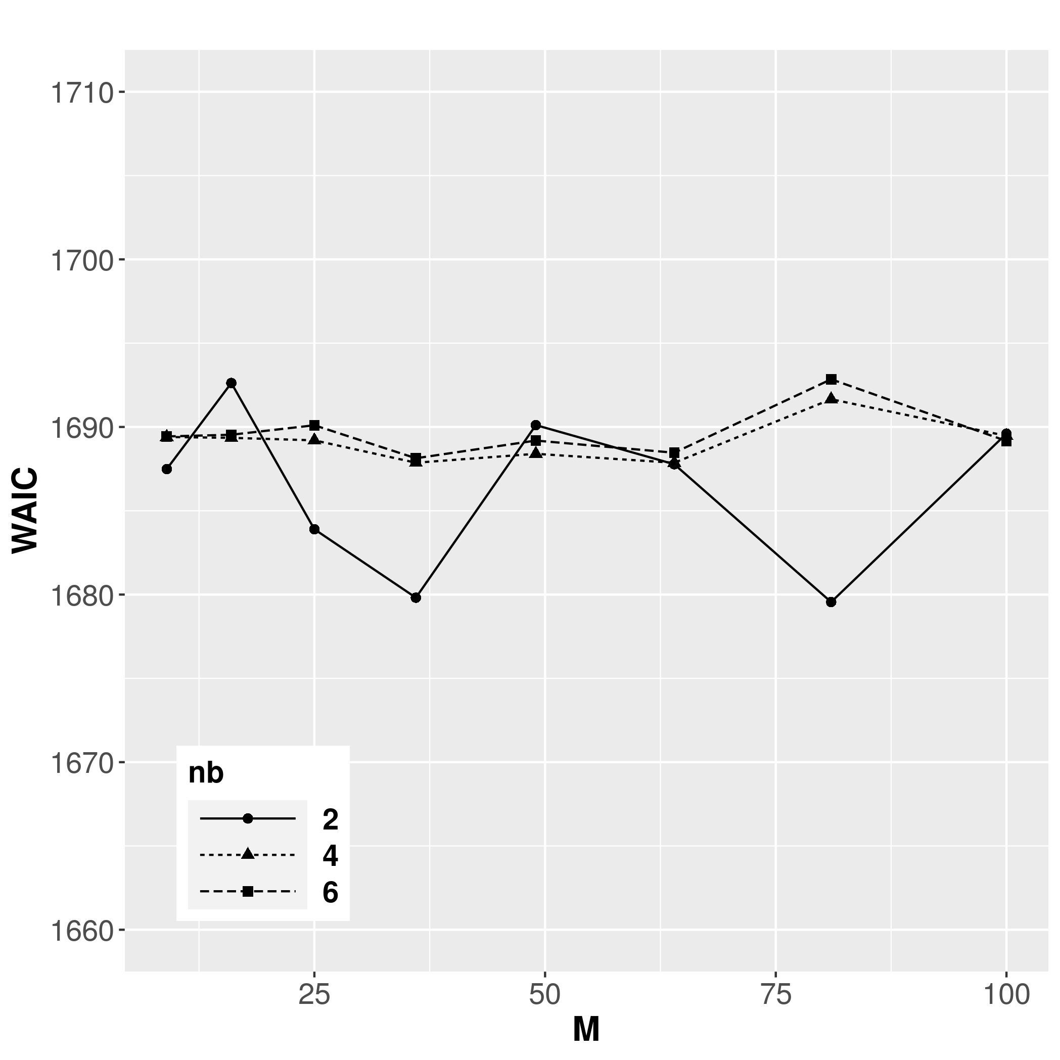
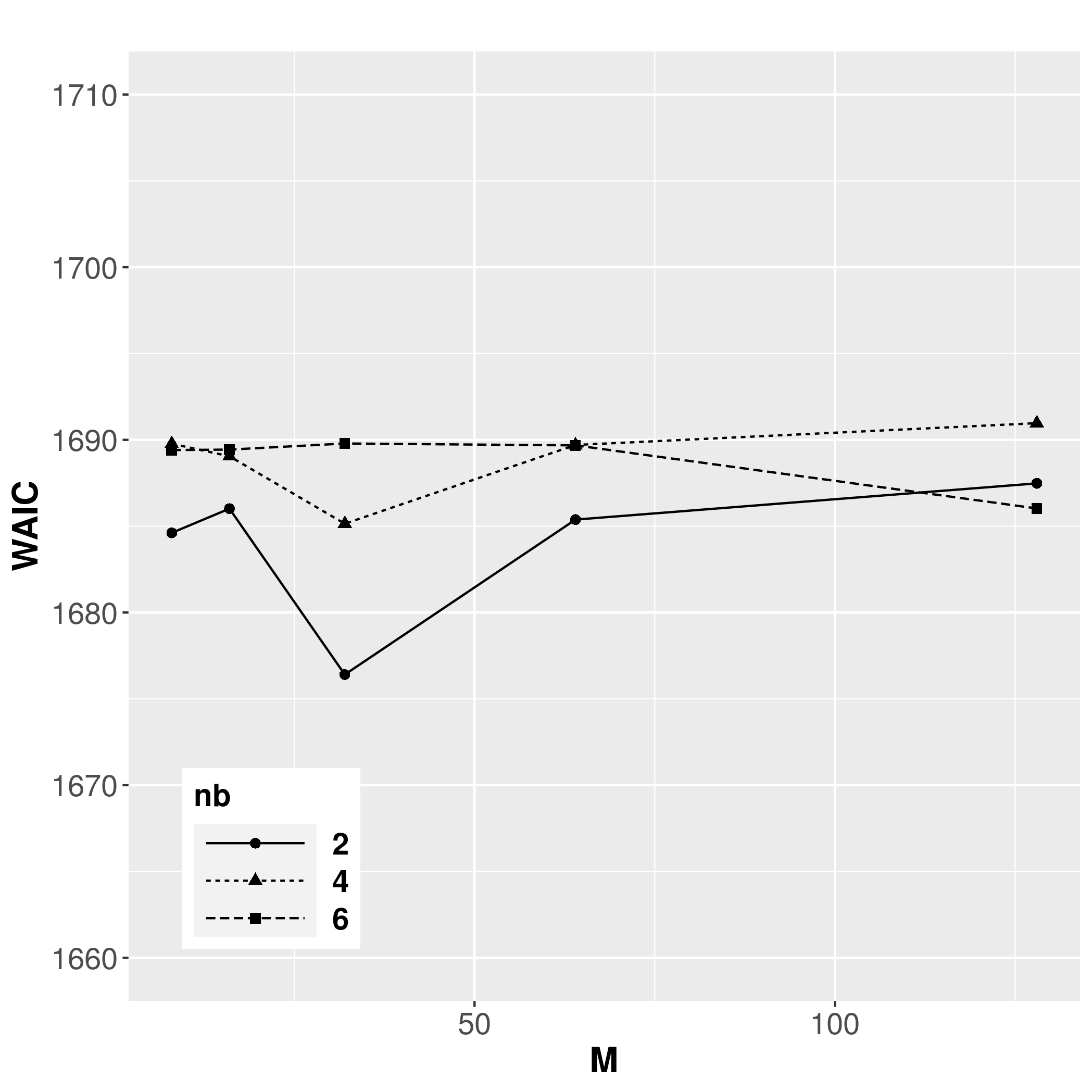
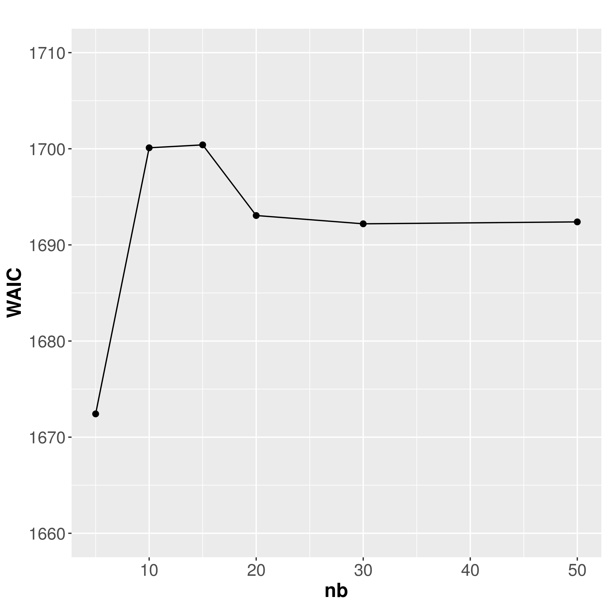
Figure 6: SIM III ($\phi$ = 3). INLA results. Criteria assessment: Running times (first row), LPML (second row) and WAIC (third row), under block-NNGP models using regular blocks (left column), irregular blocks (middle column) and NNGP models (right column).

The LPML and WAIC seems to be quite similar for block-NNGP models with $nb=4$ and $nb=6$ neighbor blocks, and the LPML shows a better goodness of fit, as well as the number of neighbors is increased. We can also observe that in general the NNGP model needs $\geq 30$ neighbors to achieve a similar goodness of fit than the block-NNGP models with $nb=4$ and $nb=6$ neighbor blocks. The WAIC of the NNGP models seems to decrease as the number of neighbors decreases, but we need to be careful because following this criteria the best model should be the NNGP model with $nb=5$ neighbors.

Parameter estimates and the root of mean square prediction error (RMSP) for specific models under SIM III ($\phi=3$) are provided in Table 2. In general, the mean posterior estimates for all the models fitted are close to the true parameter values which are included within credible intervals, but the mean posterior estimates of $\beta_{0}$ for the NNGP are far away from the true values. Further the RMSP increases when the number of blocks is increased, being lower for a higher number of neighbor blocks. This result is a little bit more evident for irregular blocks. We also found that the RSMPE for NNGP model with $10$ neighbors is lower than the RSMPE with $20$ neighbors.

Table 2: SIM III ($\phi$ = 3). INLA results. Summary of mean posterior parameter estimates, parameter posterior summary credible intervals (2.5, 97.5) and criteria assessment.

		NNGP	NNGP	(R)M=49	(R)M=64	(I)M=32	(I)M=64
		(10)	(20)	nb=4	nb=4	nb=4	nb=4
$\beta_{0}$	1	0.283	0.412	0.594	0.585	0.592	0.622
		(-0.653,1.053)	(-0.500,1.203)	(-0.321,1.501)	(-0.300,1.459)	(-0.237,1.504)	(-0.249,1.523)
$\beta_{1}$	5	4.994	4.994	4.994	4.994	4.994	4.994
		(4.977,5.011)	(4.977,5.011)	(4.977,5.011)	(4.977,5.011)	(4.977,5.011)	(4.977,5.011)
$\sigma^{2}$	1	1.081	1.044	1.053	1.045	1.019	1.036
		(0.845,1.250)	(0.813,1.208)	(0.829,1.216)	(0.815,1.209)	(0.775,1.183)	(0.804,1.200)
$\phi$	3	3.168	3.278	3.240	3.286	3.437	3.322
		(2.473,3.717)	(2.560,3.851)	(2.559,3.780)	(2.578,3.852)	(2.652,4.084)	(2.597,3.907)
$\tau^{2}$	0.1	0.092	0.092	0.092	0.092	0.091	0.092
		(0.088,0.096)	(0.088,0.096)	(0.088,0.095)	(0.088,0.095)	(0.087,0.095)	(0.088,0.095)
RMSP		0.444	0.457	0.479	0.451	0.426	0.453
Time (sec)		240.515	171.927	496.271	359.056	687.980	335.161

The previous results for large effective range are magnified when the spatial process is smoother. To illustrate this statement, we simulate data from the same model, but we set $\nu=1.5$, $\phi=3.5$, $\sigma^{2}=1$, ${\boldsymbol{\beta}}=(1,5)^{T}$ and $\tau^{2}=0.1$. We fit the next models using R-INLA: NNGP models ($nb=5,10,15,20,30,50$) and regular (R) block-NNGP models where $M=9,16,25,36,49,81,100$ and $nb=2,4,6.$ The approximate posterior marginals for the hyperparameters shows that the block-NNGP models give more accurate results than the NNGP models (Figure 7). For instance, the posterior marginals for $\tau^{2}$ with different number of blocks are overlaid, while the posterior marginals for $\sigma^{2}$ and $\phi$ with different number of blocks do not significantly change. A different result is obtained for NNGP models, where the posterior marginals for $\phi$ with different number of neighbors dramatically change.

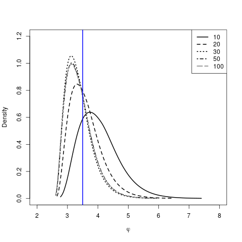
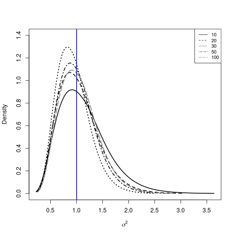
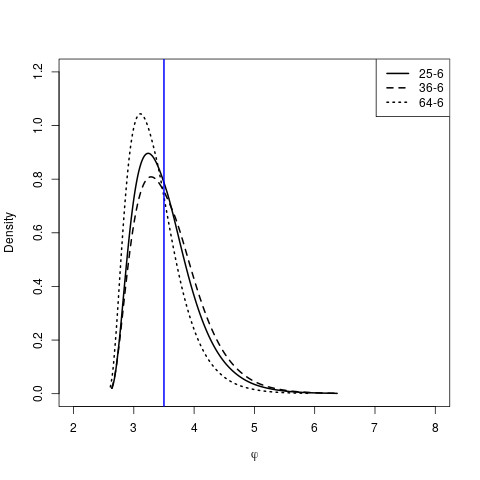
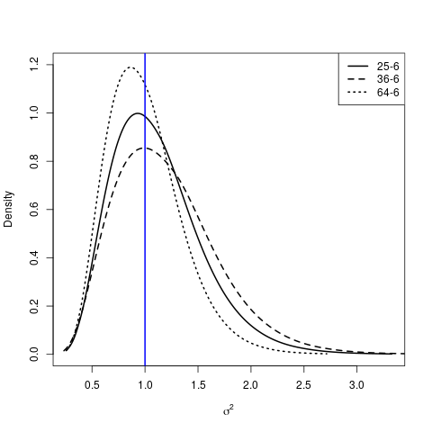
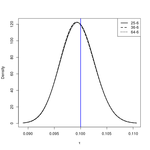
Figure 7: Posterior marginal densities of the spatial decay parameter ($\phi$), the marginal variance ($\sigma^{2}$) and nugget effect ($\tau$) for NNGP models (upper panel) with $nb=10,20,30,50,100$ neighbors and block-NNGP models (lower panel) with $M=25,36,64$ regular blocks and $nb=6$ neighbor blocks. The solid vertical blue lines represent the true parameter values.

The maps of the mean posterior estimates for block-NNGP models with regular blocks and NNGP models (Figure 8) shows the inaccuracy of NNGP models when the number of neighbors is small, they underestimate the spatial effects. In fact, a misspecified number of neighbors is more problematic for smoother processes. While the block-NNGP models show a good performance for different number of blocks. Indeed, the NNGP has proven to be successful in capturing local/small-scale variation of spatial processes, however, it might have one disadvantage: inaccuracy in representing global/large scale dependencies. This might happen because the NNGP built the DAG based on observations, adversely, the block-NNGP built a chain graph based on blocks of observations, which captures both small and large dependence.

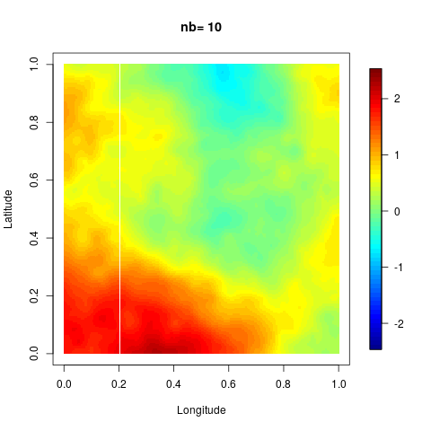
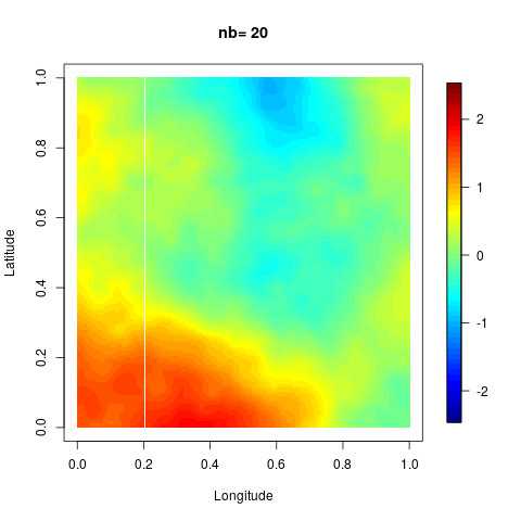
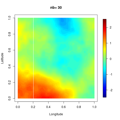
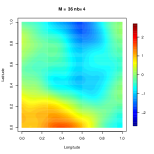
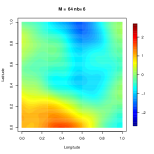
Figure 8: True spatial random effects $w$ with Matérn covariance function ($\nu=1.5$, $\phi=3.5$, $\sigma^{2}=1$ and $\tau^{2}=0.1$), and posterior mean estimates for NNGP models (upper panel) with $nb=10,20,30$ neighbors, and different block-NNGP models (lower panel) with regular blocks.

4 Applications

In this section, we illustrate the main advantages of the application of block-NNGP models throughout real data. First, the block-NNGP model is suitable for large data $(\geq 10000\mbox{ samples})$, this will be illustrated in analysing the mining data, available by Eidsvik et al., (2014). Second, the block-NNGP is suitable for data with large ranges and it can easily be combined with other model components within the general framework of latent Gaussian models and fitted efficiently using R-INLA. This is demonstrated in analysing the precipitation data in South America (available in R as noaa::cpc_pcp ).

4.1 Mining data

Here we study joint-frequency data acquired in an iron mine in the northern part of Norway (Eidsvik et al.,, 2014). We split the joint-frequency data in two subsets, a set composed by a random subset of $11000$ locations for estimation and the remaining $701$ observations were withheld to assess predictive performance. The joint-frequency data is modelled throughout a Gaussian geostatistical model, including only the effect of depth as covariate, along with an intercept, and a block-NNGP or NNGP using an exponential covariance function. The NNGP models are based on $10$ and $20$ neighbors, while the block-NNGP models are based on $280$ and $450$ regular blocks or $128$ and $289$ irregular blocks, and one neighbor block. Then we fit the models using INLA and our own implementation of the collapsed-MCMC (Finley et al.,, 2019).

Table 3 shows the parameter estimates and performance metrics, as expected, the performance of block-NNGP model is better for less blocks. We observe that the MCMC pre-processing takes approximately a month to run (based upon $10000$ iterations), while in INLA it takes a few hours or minutes. In particular, the time requirement for the block-NNGP model using irregular blocks was relatively small, although we use a small number of blocks, a possible explanation is that when using regular blocks, some blocks have a higher dimension. The goodness of fit of block-NNGP models is good, specifically for the root of mean square of error (RMSE), nevertheless, the WAIC and RSME shows a slightly better performance for NNGP models.

Table 3: Mining data. Summary of mean parameter estimates. Criteria assessment.

	INLA					MCMC
Model	NNGP	NNGP	(R)M=450	(R)M=280	(I)M=128	(I)M=289
	(20)	(10)	nb=1	nb=1	nb=1	nb=1
$\beta_{0}$	-0.022	-0.023	0.014	0.015	0.014	-0.02
$\beta_{1}$	0.0004	0.0004	0.0004	0.0004	0.0004	0.0
$\tau^{2}$	0.098	0.098	0.099	0.098	0.098	0.1
$\sigma^{2}$	0.159	0.160	0.156	0.157	0.157	0.16
$\phi$	0.074	0.072	0.074	0.075	0.076	0.07
LPML	-4913.948	-4910.236	-4983.081	-4962.783	-4957.957
WAIC2	9108.287	9123.362	9248.598	9188.431	9158.288
RMSE	0.254	0.255	0.256	0.254	0.253
RMSP	1.096	1.096	1.176	1.223	1.157
time (sec)	3030.121	2806.641	7127.620	7381.386	7573.818	2912400

We also study the predictive performance across the models. This comparison is done over 701 randomized leave-out samples. We predict the joint frequency using the predictive distribution (see Section 2.2). Among the block-NNGP models, the RMSP shows a better predictive performance of the block-NNGP model with $M=128$ irregular blocks and $nb=1$ neighbor block. Finally, maps of interpolated posterior mean estimates of joint-frequency data are displayed in the supplementary material D. We see little difference between these models. This emphasizes the small differences in the marginals for covariance parameters or the regression effects.

4.2 Precipitation data

We also analyzed the precipitation data from the National Oceanic and Atmospheric Administration (NOAA) on January, 2017, over a region covering South America. The data consist of $n=6000$ samples for estimation and $104$ to validate the models. Let $Y(s_{i})$ be the observed precipitation in the location $s_{i}$, for $i=1,\dots,n$, we assume that $Y(s_{i})\mid{\boldsymbol{x}},{\boldsymbol{\theta}}\sim\mbox{Gamma}(\mu_{i},\theta_{0})$ where $\theta_{0}$ is a precision parameter and the mean $\mu_{i}$ is defined as follows:

$$\log(\mu_{i})={\boldsymbol{Z}}^{T}(s_{i}){\boldsymbol{\beta}}+w(s_{i}),$$

where ${\boldsymbol{\beta}}$ is a vector of coefficient regression parameters, ${\boldsymbol{Z}}(s_{i})=(1,z_{1}(s_{i}))^{T}$, $z_{1}$ representing the latitude, $w(s_{i})$ is a spatial structured random effect, and the precipitation field ${\boldsymbol{w}}=(w(s_{1}),\dots,w(s_{n}))^{T}$ follows a block-NNGP or a NNGP, with a covariance function that depends on an exponential covariance function ${\boldsymbol{{C}(\sigma^{2},\phi)}}$.

We fit the block-NNGP models choosing a different number of irregular blocks $(M=64,128)$ and $nb=6$ neighbor blocks and NNGP with different number of neighbors $(nb=10,20,30,50,100)$. Full Bayesian inference was carried out using INLA. Based on the criteria assessment (see supplementary material D) the best NNGP model is the one with $nb=100$ neighbors, followed by the model with $nb=20$ neighbors. While the best block-NNGP model is the one with $M=64$ and $nb=4$ neighbor blocks. Overall, the results are more stable for less blocks and more neighbor blocks. The RSME is lower for block-NNGP models. Note that all the models run in a reasonable time, for instance the block-NNGP model with $M=64$ and $nb=4$ neighbor blocks (with approximately $376$ neighbors) runs in 13587.350 seconds.

Figure (9) displays the marginal posterior densities for the $\phi$ and $\sigma^{2}$. We observe that there is not a clear pattern for NNGP models, for a small number of neighbors ($10$ and $20$), the mean posterior of $\phi$ hits the boundary of its prior uniform distribution, it increases for $30$ and $50$ neighbors, but it decreases again for $100$ neighbors. A similar pattern is observed for $\sigma^{2}$. While, the block-NNGP models with a considerable number of neighbor blocks, ensures a quite similar estimation of $\phi$ and $\sigma^{2}$. Posterior means of the spatial fields under different models are also shown in Figure (9).

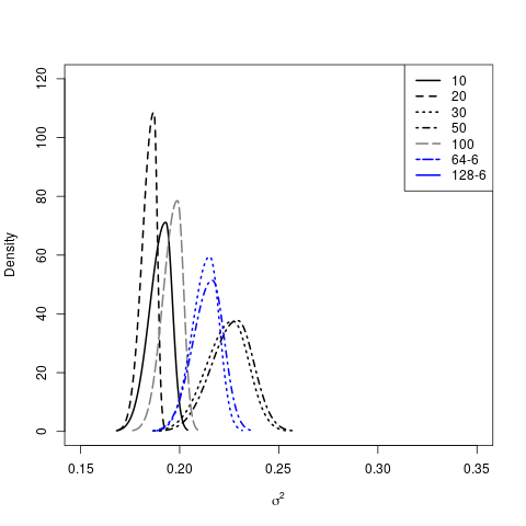
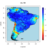
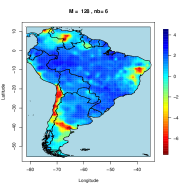
Figure 9: First column: Posterior marginal densities of the spatial decay parameter $\phi$ and the marginal variance $\sigma^{2}$ for NNGP models with $nb=10,20,30,50,100$ neighbors and block-NNGP models with $M=64,128$ irregular blocks and $nb=6$ neighbor blocks. Second column: Posterior mean estimates of spatial random effects for NNGP models. Third column: Posterior mean estimates of spatial random effects of block-NNGP models.

5 Conclusion

This paper introduces the block-NNGP, a new GMRF for approximating Gaussian processes. An important feature is that this process is valid for any covariance function. Moreover, the precision matrix of the block-NNGP has a block-sparse structure, which allows scalable inference and distributed computations. Although there might not be an explicit number of blocks and neighbor blocks for optimal blocking, we are able to determine an adequate one by comprising the computational speed and statistical efficiency. Further, inference can be performed by the use of MCMC methods as well as the INLA approach (Rue et al.,, 2009). However, we advocate the use of the INLA methodology.

INLA requires the latent field to be a GMRF as in our proposal, hence it provides a huge computational benefit, providing precise estimates in seconds or minutes. Furthermore, the combination of INLA and the block-NNGP directly allows for fast inference for non-Gaussian observations (e.g., Section 4.2). Scalable models for massive non-Gaussian data have been a challenge in the literature (Lee and Haran,, 2019) with very few option available, we believe that the block-NNGP within INLA is an interesting alternative to perform such modeling in massive dataset preserving the characteristics of the data, e.g, avoiding transformation to achieve normality.

Using theoretical results, large simulated data and real-data applications we have shown that the block-NNGP can provide a good approximation at low computational complexity and time. In particular, the block-NNGP performs better than the NNGP when the range is large or the spatial process is smoother. Extension of the block-NNGP process, e.g., multivariate and spatio-temporal extensions, will be investigated in future works.

SUPPLEMENTARY MATERIAL

The supplementary material presents the formal proofs of the Theorems, Lemmas and Prepositions. Also, the full-MCMC algorithm is proposed. Finally, detailed simulation and application results are discussed.

SUPPLEMENTARY MATERIAL

A. Proofs of main results

Matrix Analysis Background
Theorem A1: A matrix ${\boldsymbol{B}}\in{\boldsymbol{\Re}}^{m\times n}$ is full column rank if and only if ${\boldsymbol{B^{T}B}}$ is invertible
Theorem A2: The determinant of an $n\times n$ matrix ${\boldsymbol{B}}$ is 0 if and only if the matrix ${\boldsymbol{B}}$ is not invertible.
Theorem A3: Let ${\boldsymbol{T_{n}}}$ be a triangular matrix (either upper or lower) of order n. Let $\det({\boldsymbol{T_{n}}})$ be the determinant of ${\boldsymbol{T_{n}}}$. Then $\det({\boldsymbol{T_{n}}})$ is equal to the product of all the diagonal elements of ${\boldsymbol{T_{n}}},$ that is, $\det({\boldsymbol{T_{n}}})=\prod_{k=1}^{n}(a_{kk}).$
Proposition A1: If ${\boldsymbol{B}}$ is positive definite (p.d.), then if ${\boldsymbol{S}}$ has full column rank, then ${\boldsymbol{S^{T}BS}}$ is positive definite.
Corollary A1: If ${\boldsymbol{B}}$ is positive definite, then ${\boldsymbol{B^{-1}}}$ is positive definite.

Proof of Proposition 1.

If $\pi({\boldsymbol{w_{S}}})$ is a valid multivariate joint density, $\pi({\boldsymbol{{w}_{b_{k}}}}|{\boldsymbol{{w}_{N(b_{k})}}})$ is also proper, and we have that $\int\pi({\boldsymbol{w_{b_{k}}}}|{\boldsymbol{w_{N(b_{k})}}})d{\boldsymbol{w_{b_{k}}}}=1,\forall k=1,\dots,M.$ From the definitions of ${\boldsymbol{G}}$ and ${\boldsymbol{G^{b}}}$ there exists a set of nodes in block $\Delta(b_{1})$, ${\boldsymbol{s_{\Delta(b_{1})}}}\in{\boldsymbol{G}}$, such that “the last node” from a DAG ${\boldsymbol{G^{b}}}$ belongs to ${\boldsymbol{s_{\Delta(b_{1})}}}$. Then the nodes in ${\boldsymbol{s_{\Delta(b_{1})}}}$ do not have any directed edge originating from them. As a consequence, any node in block $\Delta(b_{1})$ can not belong to the set of nodes of any other block. So the term in (2) where all locations of ${\boldsymbol{\Delta(b_{1})}}$ appear is $\pi({\boldsymbol{w_{\Delta(b_{1})}}}|{\boldsymbol{w_{N(\Delta(b_{1}))}}})$. From Fubini’s theorem, we can interchange the product and integral, thus

$$\int{\pi}({\boldsymbol{w_{S}}})d{\boldsymbol{w_{S}}} = \int\dots\int\prod_{i=1}^{M}\pi({\boldsymbol{w_{\Delta(b_{i})}}}|{\boldsymbol{w_{N(\Delta(b_{i}))}}})d{\boldsymbol{w_{\Delta(i)}}}$$

$$= \int\dots\int\prod_{i=2}^{M}\pi({\boldsymbol{w_{\Delta(b_{i})}}}|{\boldsymbol{w_{N(\Delta(b_{i}))}}})d{\boldsymbol{w_{\Delta(i)}}}.$$

Then, removing every node of ${\boldsymbol{\Delta(b_{1})}}$ from ${\boldsymbol{G}}$ and ${\boldsymbol{G^{b}}}$, we have the chain graph ${\boldsymbol{G^{\prime}}}$ and DAG ${\boldsymbol{G^{\prime}_{b}}}$, respectively. There exists another set of nodes ${\boldsymbol{s_{\Delta(b_{2})}}}$ in ${\boldsymbol{G^{\prime}}}$, such that “the last node” from a DAG ${\boldsymbol{G^{\prime}_{b}}}$ belongs to ${\boldsymbol{s_{\Delta(b_{2})}}}$. Then the nodes ${\boldsymbol{s_{\Delta(b_{2})}}}$ do not have any directed edge originating from them. As consequence, any node in block ${\boldsymbol{\Delta(b_{2})}}$ can not belong to the set of nodes of any other block. So the term in (2) where all locations of ${\boldsymbol{\Delta(b_{2})}}$ appear is $\pi({\boldsymbol{w_{\Delta(b_{2})}}}|{\boldsymbol{w_{N(\Delta(b_{2}))}}})$. Applying the Fubini’s theorem again,

$$\int\pi({\boldsymbol{w_{S}}})d{\boldsymbol{w_{S}}} = \int\dots\int\prod_{i=3}^{M}\pi({\boldsymbol{w_{\Delta(b_{i})}}}|{\boldsymbol{w_{N(\Delta(b_{i}))}}})d{\boldsymbol{w_{\Delta(i)}}}.$$

In a similar way, we find ${\boldsymbol{s_{\Delta(b_{3})}}},\dots,{\boldsymbol{s_{\Delta(M)}}}$, such that,
$\int\pi({\boldsymbol{w_{S}}})d{\boldsymbol{w_{S}}}=\int\prod_{i=1}^{M}\pi({\boldsymbol{w_{\Delta(b_{i})}}}|{\boldsymbol{w_{N(\Delta(b_{i}))}}})d{\boldsymbol{w_{\Delta(i)}}}=1.$ ∎

Proof of Proposition 2.

Without loss of generality, assume that the data were reordered by blocks. From known properties of Gaussian distributions, ${\boldsymbol{w_{b_{k}}}}|{\boldsymbol{w_{N(b_{k})}}}\sim N({\boldsymbol{B_{b_{k}}}}{\boldsymbol{w_{N(b_{k})}}},{\boldsymbol{F_{b_{k}}}})$, where ${\boldsymbol{B_{b_{k}}}}={\boldsymbol{C_{b_{k},N(b_{k})}}}{\boldsymbol{C^{-1}_{N(b_{k})}}}$ and ${\boldsymbol{F_{b_{k}}}}={\boldsymbol{C_{b_{k}}}}-{\boldsymbol{C_{b_{k},N(b_{k})}}}{\boldsymbol{C^{-1}_{N(b_{k})}}}{\boldsymbol{C_{N(b_{k}),b_{k}}}}.$ Hence,

$$\widetilde{\pi}({\boldsymbol{w_{S}}}) = \prod_{k=1}^{M}p({\boldsymbol{w_{b_{k}}}}|{\boldsymbol{w_{N(b_{k})}}})$$

$$\propto \prod_{k=1}^{M}\frac{1}{|{\boldsymbol{F_{b_{k}}}}|^{1/2}}\exp\left\{-\frac{1}{2}({\boldsymbol{w_{b_{k}}}}-{\boldsymbol{B_{b_{k}}}}{\boldsymbol{w_{N(b_{k})}}})^{T}{\boldsymbol{F_{b_{k}}}}^{-1}({\boldsymbol{w_{b_{k}}}}-{\boldsymbol{B_{b_{k}}}}{\boldsymbol{w_{N(b_{k})}}})\right\}$$

$$\propto \frac{1}{\prod_{k=1}^{M}|{\boldsymbol{F_{b_{k}}}}|^{1/2}}\exp\left\{-\frac{1}{2}\sum_{k=1}^{M}({\boldsymbol{w_{b_{k}}}}-{\boldsymbol{B_{b_{k}}}}{\boldsymbol{w_{N(b_{k})}}})^{T}{\boldsymbol{F_{b_{k}}}}^{-1}({\boldsymbol{w_{b_{k}}}}-{\boldsymbol{B_{b_{k}}}}{\boldsymbol{w_{N(b_{k})}}})\right\}.$$

Let ${\boldsymbol{w_{b_{k}}}}-{\boldsymbol{B_{b_{k}}}}{\boldsymbol{w_{N(b_{k})}}}={\boldsymbol{B^{\star}_{b_{k}}}}{\boldsymbol{w_{S}}}$, and $j$ be the $j$-$th$ observation of block ${\boldsymbol{b_{k}}}$, then $\forall k=1,\dots,M$, $i=1,\dots,n$ and $j=1,\dots,n_{bk}$:

$$B^{\star}_{b_{k}}(j,i)=\begin{cases}1&\quad\text{if }s_{i}\in{\boldsymbol{s_{b_{k}}}}\\ B_{b_{i}}[j,l]&\quad\text{if }s_{i}\in{\boldsymbol{s_{b_{k}}}};s_{i}=s_{N(b_{k})}[l];l=1,\dots,N_{bk}\\ 0&\quad\text{otherwise,}\end{cases}$$

and

$${\boldsymbol{B^{\star}_{b_{k}}}}=\begin{bmatrix}{\boldsymbol{B^{\star}_{b_{k}}(1)}}\\ \vdots\\ {\boldsymbol{B^{\star}_{b_{k}}(j)}}\\ \vdots\\ {\boldsymbol{B^{\star}_{b_{k}}(n_{b_{k}})}}\end{bmatrix}_{n_{b_{k}}\times n},$$

where ${\boldsymbol{B^{\star}_{b_{k}}(j)}}=(B^{\star}_{b_{k}}(j,1),B^{\star}_{b_{k}}(j,2),\dots,B^{\star}_{b_{k}}(j,n))$. From these definitions, ${\boldsymbol{B^{\star}_{b_{k}}}}$ is a matrix with i-th column full of zeros if $s_{i}\notin{\boldsymbol{s_{b_{k}}}}$ or $s_{i}\notin{\boldsymbol{N(s_{b_{k}})}}$. Since the data were reordered by blocks and the neighbor blocks are from the past, ${\boldsymbol{B^{\star}_{b_{k}}}}$ has also the next form:

$${\boldsymbol{B^{\star}_{b_{k}}}}=\left[\begin{array}[]{ccccc}{\boldsymbol{R_{k}}}&{\boldsymbol{A_{k}}}&0&\dots&0\\ \cline{2-2}\cr\end{array}\right],$$

where ${\boldsymbol{A_{k}}}$ is a $n_{bk}\times n_{bk}$ matrix and ${\boldsymbol{R_{k}}}$ is a $n_{bk}\times\sum_{r=1}^{k-1}n_{br}$ matrix with at least one column with none null-element if $nb\neq 0$.
Then,

$$\widetilde{\pi}({\boldsymbol{w_{S}}}) \propto \frac{1}{\prod_{k=1}^{M}|{\boldsymbol{F_{b_{k}}}}|^{1/2}}\exp\left\{-\frac{1}{2}\sum_{k=1}^{M}({\boldsymbol{B^{\star}_{b_{k}}}}{\boldsymbol{w_{S}}})^{T}{\boldsymbol{F_{b_{k}}^{-1}}}({\boldsymbol{B^{\star}_{b_{k}}}}{\boldsymbol{w_{S}}})\right\}$$

$$\propto \frac{1}{\prod_{k=1}^{M}|{\boldsymbol{F_{b_{k}}}}|^{1/2}}\exp\left\{-\frac{1}{2}\sum_{k=1}^{M}{\boldsymbol{w_{S}^{T}}}({\boldsymbol{B_{b_{k}}^{\star}}})^{T}{\boldsymbol{F_{b_{k}}^{-1}}}({\boldsymbol{B^{\star}_{b_{k}}}}{\boldsymbol{w_{S}}})\right\}$$

$$\propto \frac{1}{\prod_{k=1}^{M}|{\boldsymbol{F_{b_{k}}}}|^{1/2}}\exp\left\{-\frac{1}{2}\sum_{k=1}^{M}{\boldsymbol{w_{S}^{T}}}(({\boldsymbol{B_{b_{k}}^{\star}}})^{T}{\boldsymbol{F_{b_{k}}^{-1}}}{\boldsymbol{B_{b_{k}}}}^{\star}){\boldsymbol{w_{S}}}\right\}$$

$$\propto \frac{1}{\prod_{k=1}^{M}|{\boldsymbol{F_{b_{k}}}}|^{1/2}}\exp\left\{-\frac{1}{2}{\boldsymbol{w_{S}}}^{T}(\sum_{k=1}^{M}({\boldsymbol{B_{b_{k}}}}^{\star})^{T}{\boldsymbol{F_{b_{k}}^{-1}}}{\boldsymbol{B_{b_{k}}}}^{\star}){\boldsymbol{w_{S}}}\right\}.$$

Let $\sum_{k=1}^{M}({\boldsymbol{B_{b_{k}}}}^{\star})^{T}{\boldsymbol{F^{-1}_{b_{k}}}}{\boldsymbol{B_{b_{k}}}}^{\star}=({\boldsymbol{B^{\star}_{s}}})^{T}{\boldsymbol{F_{s}^{-1}}}{\boldsymbol{B^{\star}_{s}}}$, where ${\boldsymbol{B_{s}}}=\left[\begin{array}[]{ccccc}{\boldsymbol{B_{b1}^{\star}}}&...&...&\dots&{\boldsymbol{B_{bM}^{\star}}}\\ \end{array}\right]$ and ${\boldsymbol{F_{s}^{-1}}}=\mbox{diag}({\boldsymbol{F_{b_{k}}^{-1}}})$. ${\boldsymbol{F_{s}^{-1}}}$ is a block diagonal matrix and (iii) is proved. And given that ${\boldsymbol{B^{\star}_{b_{k}}}}$ is a matrix with i-th column full of zeros for $i>\sum_{r=1}^{k}n_{br}$, then ${\boldsymbol{B_{s}}}$ is a block matrix and lower triangular, and (ii) is proved.
Finally, $\widetilde{p}({\boldsymbol{w_{S}}})\propto\frac{1}{\prod_{k=1}^{M}|{\boldsymbol{F_{b_{k}}}}|^{1/2}}\exp\left\{-\frac{1}{2}{\boldsymbol{w_{S}^{T}}}({\boldsymbol{B_{s}^{T}F_{s}^{-1}B_{s}}}){\boldsymbol{w_{S}}}\right\}$ and ${\boldsymbol{\widetilde{C}_{s}^{-1}}}={\boldsymbol{\widetilde{Q}_{s}}}={\boldsymbol{B_{s}^{T}F_{s}^{-1}B_{s}}}.$

$\widetilde{C}_{s}$ is positive definite
From properties of the Normal distribution, the covariance of the conditional distribution of ${\boldsymbol{w_{b_{k}}}}|{\boldsymbol{w_{N(b_{k})}}}$ is also p.d. (by Schur complement conditions), then ${\boldsymbol{F_{bk}}}={\boldsymbol{C_{b_{k}}}}-{\boldsymbol{C_{b_{k},N(b_{k})}}}{\boldsymbol{C^{-1}_{N(b_{k})}}}{\boldsymbol{C_{N(b_{k}),b_{k}}}}$, is p.d. Moreover, ${\boldsymbol{F_{s}}}=diag({\boldsymbol{F_{bk}}})$ and a block diagonal matrix is p.d. iff each diagonal block is positive definite, so given that ${\boldsymbol{F_{bk}}}$ is p.d. and ${\boldsymbol{F_{s}}}$ is block diagonal with blocks ${\boldsymbol{F_{bk}}}$ p.d then ${\boldsymbol{F_{s}}}$ is p.d. By Corollary A1, ${\boldsymbol{F_{s}}}$ is p.d. then ${\boldsymbol{F^{-1}_{s}}}$ is p.d. By Theorem A1, ${\boldsymbol{B_{s}}}$ has full column rank if and only iff ${\boldsymbol{R_{s}}}={\boldsymbol{B^{T}_{s}B_{s}}}$ is invertible. By Theorem A2, the inverse of ${\boldsymbol{R_{s}}}$ exists if and only if $\det({\boldsymbol{R_{s}}})\neq 0$. Using the well-known matrix theorems, we can prove the following: $\det({\boldsymbol{R_{s}}})=\det({\boldsymbol{B^{T}_{s}B_{s}}})=\det({\boldsymbol{B^{T}_{s}}})\det({\boldsymbol{B_{s}}})\neq 0$ if $\det({\boldsymbol{B^{T}_{s}}})=\det({\boldsymbol{B_{s}}})\neq 0$. Given that ${\boldsymbol{B_{s}}}$ is a lower triangular matrix, by Theorem A3, $\det({\boldsymbol{B_{s}}})=\prod_{k=1}^{n}(b_{kk})$. And, $b_{kk}=1,\forall k$, then $\det({\boldsymbol{B_{s}}})\neq 0.$ So, ${\boldsymbol{R_{s}}}$ is invertible and ${\boldsymbol{B_{s}}}$ has full column rank. By Proposition A1, given that ${\boldsymbol{B_{s}}}$ has full column rank, and ${\boldsymbol{F_{s}^{-1}}}$ is p.d. then ${\boldsymbol{\widetilde{Q}_{s}}}={\boldsymbol{\widetilde{C}_{s}^{-1}}}={\boldsymbol{B^{T}_{s}F_{s}^{-1}B_{s}}}$ is p.d. Also by corollary A1, ${\boldsymbol{\widetilde{C}_{s}^{-1}}}$ is p.d. then ${\boldsymbol{\widetilde{C}_{s}}}$ is p.d.

Since $\widetilde{p}({\boldsymbol{w_{S}}})\propto\frac{1}{\prod_{k=1}^{M}|{\boldsymbol{F_{b_{k}}}}|^{1/2}}\exp\left\{-\frac{1}{2}{\boldsymbol{w_{S}}}^{T}({\boldsymbol{\widetilde{C}_{s}}}^{-1}){\boldsymbol{w_{S}}}\right\}$, ${\boldsymbol{\widetilde{C}_{s}}}^{-1}={\boldsymbol{B_{s}^{T}F_{s}^{-1}B_{s}}}$, and ${\boldsymbol{\widetilde{C}_{s}}}$ is p.d., then $\widetilde{p}({\boldsymbol{w_{S}}})$ is a pdf of a multivariate normal distribution.

If $n_{bk}\ll n$ then $i>\sum_{r=1}^{k}n_{br}$ and ${\boldsymbol{B^{\star}_{b_{k}}}}$ will be more sparse. Also, if $n_{k}$ is small, the block diagonal matrix ${\boldsymbol{F_{s}}}^{-1}$ will be more sparse. As a result, ${\boldsymbol{\widetilde{C}_{s}^{-1}}}={\boldsymbol{B_{s}^{T}F_{s}^{-1}B_{s}}}$, will still be sparse. ∎

Proof of Lemma 1.

We need to prove that the finite dimensional distributions in (6) are consistent with a stochastic process. The Kolmogorov consistency conditions are checked as follows:

Symmetry under permutation: Let $\Delta_{1},\dots,\Delta_{n}$ be any permutation of $1,\dots,n$, note that ${\boldsymbol{S}}$ is fixed, then it is clear that $\widetilde{\pi}(w{(v_{1})},\dots,w{(v_{n})})=\widetilde{\pi}(w{(v_{\Delta_{1}})},\dots,w{(v_{\Delta_{n}}}))$ if and only if the same holds for the distribution of $u_{i}|{\boldsymbol{N(u_{i})}}$. Since ${\boldsymbol{w_{U}}}|{\boldsymbol{w_{S}}}$ follows a l-multivariate normal distribution, then the symmetry condition is satisfied by $\pi({\boldsymbol{w_{U}}}|{\boldsymbol{w_{S}}})$, and it holds that the next condition $\widetilde{\pi}({w{(u_{1})}},\dots,{w{(u_{l})}}|{\boldsymbol{w_{S}}})=\widetilde{\pi}({w{(u_{\Delta_{1}})}},\dots,{w{(u_{\Delta_{l}}}})|{\boldsymbol{w_{S}}})$ is necessary and sufficient to prove the symmetry condition of $\widetilde{\pi}({\boldsymbol{w_{V}}})$. To prove this we define the next pdfs,

$$\widetilde{\pi}(w(u_{1}),\dots,w(u_{l})|{\boldsymbol{w_{S}}}) = |2\pi{\boldsymbol{F_{U}}}|^{-1/2}\exp\left\{-\frac{1}{2}({\boldsymbol{w_{U}}}-{\boldsymbol{B_{U}w_{S}}})^{T}{\boldsymbol{F_{U}}}^{-1}({\boldsymbol{w_{U}}}-{\boldsymbol{B_{U}w_{S}}})\right\}$$

$$= |2\pi{\boldsymbol{F_{U}}}|^{-1/2}\exp\left\{{\boldsymbol{Q(w_{U})}}\right\},$$

and

$$\widetilde{p}(w(u_{\Delta_{1}}),\dots,w(u_{\Delta_{l}})|{\boldsymbol{w_{S}}}) = |2\pi{\boldsymbol{\Sigma^{\prime}}}|^{-1/2}\exp\left\{-\frac{1}{2}({\boldsymbol{w_{U\Delta}}}-{\boldsymbol{m^{\prime}}})^{T}{{\boldsymbol{\Sigma^{\prime}}}}^{-1}({\boldsymbol{w_{U\Delta}}}-{\boldsymbol{m^{\prime}}})\right\}$$

$$= |2\pi{\boldsymbol{\Sigma^{\prime}}}|^{-1/2}\exp\left\{{\boldsymbol{Q(w_{U\Delta}}})\right\}.$$

following Abrahamsen, (1997), we also define a permutation matrix ${\boldsymbol{P}}$ such that $(\Delta_{1},\dots,\Delta_{l})^{T}={\boldsymbol{P}}(1,\dots,l)^{T}$. Then ${\boldsymbol{P}}w_{U}={\boldsymbol{P}}(w(u_{1}),\dots,w(u_{l}))^{T}=(w(u_{\Delta_{1}}),\dots,w(u_{\Delta_{l}}))^{T}={\boldsymbol{w_{U\Delta}}}$. And the mean and covariance matrix of ${\boldsymbol{w_{U}{\Delta}}}|{\boldsymbol{w_{S}}}$ are ${\boldsymbol{m^{\prime}}}={\boldsymbol{PB_{U}w_{S}}}$ and ${\boldsymbol{\Sigma^{\prime}}}={\boldsymbol{PF_{U}P^{\prime}}}$. Since ${\boldsymbol{P}}^{-1}={\boldsymbol{P}}^{T}$ it follows that $|{\boldsymbol{P}}|=\pm 1$ which implies that $|{\boldsymbol{\Sigma^{\prime}}}|=|{\boldsymbol{F_{U}}}|$. Using this we have,

$${\boldsymbol{Q(w_{U\Delta})}} =({\boldsymbol{Pw_{U}-m^{\prime}}})^{T}{\boldsymbol{\Sigma^{\prime}}}^{-1}({\boldsymbol{Pw_{U}-m^{\prime}}})$$

$$=({\boldsymbol{Pw_{U}-PB_{U}w_{S}}})^{T}({\boldsymbol{PF_{U}P^{\prime}}})^{-1}({\boldsymbol{Pw_{U}}}-{\boldsymbol{PB_{U}w_{S}}})$$

$$=({\boldsymbol{w_{U}}}-{\boldsymbol{B_{U}w_{S}}})^{T}{\boldsymbol{P}}^{T}({\boldsymbol{P}}^{T}{\boldsymbol{F_{U}}}^{-1}{\boldsymbol{P}}^{T}){\boldsymbol{P}}({\boldsymbol{w_{U}}}-{\boldsymbol{B_{U}w_{S}}})$$

$$=({\boldsymbol{w_{U}}}-{\boldsymbol{B_{U}w_{S}}})^{T}{\boldsymbol{P}}^{T}{\boldsymbol{\Sigma^{\prime}}}^{-1}{\boldsymbol{P}}({\boldsymbol{w_{U}}}-{\boldsymbol{B_{U}w_{S}}})$$

$$=({\boldsymbol{w_{U}}}-{\boldsymbol{B_{U}w_{S}}})^{T}{\boldsymbol{F_{U}}}^{-1}({\boldsymbol{w_{U}}}-{\boldsymbol{B_{U}w_{S}}})={\boldsymbol{Q(w_{U})}}.$$

Since both $|{\boldsymbol{F_{U}}}|$ and ${\boldsymbol{Q(w_{U})}}$ are invariant under permutations, $\widetilde{\pi}(w{(u_{1})},\dots,w{(u_{l})}|{\boldsymbol{w_{S}}})=\widetilde{\pi}(w{(u_{\Delta_{1}})},\dots,w{(u_{\Delta_{l}}})|{\boldsymbol{w_{S}}})$ and hence the symmetry condition is satisfied.

Dimensional consistency: We also assume that ${\boldsymbol{S}}$ is fixed, so, this proof does not differ from the one found in (Datta et al.,, 2016) although $\widetilde{\pi}({\boldsymbol{w_{S}}})$ has a different definition.
Let ${\boldsymbol{V_{1}}}={\boldsymbol{V}}\cup\{v_{0}\}$ then ${\boldsymbol{V_{1}}}={\boldsymbol{S^{\prime}}}\cup\{v_{0}\}\cup{\boldsymbol{U}}$. We need to verify $\widetilde{\pi}({\boldsymbol{w_{V}}})=\int\widetilde{\pi}({\boldsymbol{w_{V_{1}}}})d(w(v_{0}))$. So, we have two cases:
Case 1: If $v_{0}\in{\boldsymbol{S}}$. By definition $\widetilde{\pi}({\boldsymbol{w_{V_{1}}}})=\int\widetilde{\pi}({\boldsymbol{w_{{V_{1}}|{\boldsymbol{S}}}}}|{\boldsymbol{w_{S}}})\widetilde{p}({\boldsymbol{w_{S}}})\prod_{si\in{\boldsymbol{S}}|{\boldsymbol{V_{1}}}}d(w_{s_{i}})$, where ${V_{1}}|{\boldsymbol{S}}$ denotes ${V_{1}}$ without ${\boldsymbol{S}}$ and ${\boldsymbol{S}}|{V_{1}}$ denotes ${\boldsymbol{S}}$ without ${V_{1}}$. Then

$$\int\widetilde{\pi}({\boldsymbol{w_{V_{1}}}})d(w(v_{0}))=\int\widetilde{\pi}({\boldsymbol{w_{{V_{1}}|{\boldsymbol{S}}}|{\boldsymbol{w_{S}}}}})\widetilde{\pi}({\boldsymbol{w_{S}}})\prod_{si\in{\boldsymbol{S}}|{\boldsymbol{V_{1}}}}d(w(s_{i}))d(w(v_{0})).$$

If $v_{0}\in{\boldsymbol{S}}$, and ${\boldsymbol{V}}={\boldsymbol{S^{\prime}}}\cup{\boldsymbol{U}}$ then $v_{0}\in({\boldsymbol{S^{\prime}}})^{c}$, and $\prod_{si\in{\boldsymbol{S}}|{\boldsymbol{V_{1}}}}d(w(s_{i})d(w(v_{0}))=\prod_{si\in({\boldsymbol{S^{\prime}}})^{c}}d(w(s_{i})$, and

$$\int\widetilde{\pi}(w_{{\boldsymbol{V_{1}}}})d(w(v_{0}))=\int\widetilde{\pi}({\boldsymbol{w_{V_{1}|S}}}|{\boldsymbol{w_{S}}})\widetilde{\pi}({\boldsymbol{w_{S}}})\prod_{si\in({\boldsymbol{S^{\prime}}})^{c}}d(w_{s_{i}}).$$

Also, ${{\boldsymbol{V_{1}}}|{\boldsymbol{S}}}={\boldsymbol{U}}$ since $v_{0}\in{\boldsymbol{S}}$, then

$$\int\widetilde{\pi}({\boldsymbol{w_{V_{1}}}})d(w(v_{0}))=\int\widetilde{\pi}({\boldsymbol{w_{U}}}|{\boldsymbol{w_{S}}})\widetilde{\pi}({\boldsymbol{w_{S}}})\prod_{si\in({\boldsymbol{S^{\prime}}})^{c}}d(w_{s_{i}})=\widetilde{\pi}({\boldsymbol{w_{V}}}).$$

Case 2: If $v_{0}\notin{\boldsymbol{S}}$, then ${\boldsymbol{V_{1}}}|{\boldsymbol{S}}={\boldsymbol{U}}\cup\{v_{0}\}$, $\widetilde{\pi}({\boldsymbol{w_{V_{1}|S}}}|{\boldsymbol{w_{S}}})=\widetilde{\pi}({\boldsymbol{w_{U|S}}}|{\boldsymbol{w_{S}}})\widetilde{\pi}(w(v_{0})|{\boldsymbol{w_{S}}})$ and ${\boldsymbol{S|V_{1}}}=({\boldsymbol{S^{\prime}}})^{c}$. Now,

$$\widetilde{\pi}({\boldsymbol{w_{V_{1}}}}) = \int\widetilde{\pi}({\boldsymbol{w_{V_{1}|S}}}|{\boldsymbol{w_{S}}})\widetilde{\pi}({\boldsymbol{w_{S}}})\prod_{si\in{\boldsymbol{S}}|{\boldsymbol{V_{1}}}}d(w_{s_{i}})$$

$$= \int\ \widetilde{\pi}({\boldsymbol{w_{U}}}|{\boldsymbol{w_{S}}})\widetilde{\pi}(w(v_{0})|{\boldsymbol{w_{S}}})\widetilde{\pi}({\boldsymbol{w_{S}}})\prod_{si\in({\boldsymbol{S^{\prime}}})^{c}}d(w_{s_{i}}).$$

Hence,

$$\int\widetilde{\pi}({\boldsymbol{w_{V_{1}}}})d(w(v_{0})) = \int\widetilde{\pi}({\boldsymbol{w_{U}}}|{\boldsymbol{w_{S}}})\widetilde{\pi}(w(v_{0})|{\boldsymbol{w_{S}}})\widetilde{\pi}({\boldsymbol{w_{S}}})\prod_{si\in({\boldsymbol{S^{\prime}}})^{c}}d(w_{s_{i}})d(w(v_{0}))$$

$$= \int\widetilde{\pi}({\boldsymbol{w_{S}}})\widetilde{\pi}({\boldsymbol{w_{U}}}|{\boldsymbol{w_{S}}})[\widetilde{\pi}(w(v_{0})|{\boldsymbol{w_{S}}})d(w(v_{0}))]\prod_{si\in({\boldsymbol{S^{\prime}}})^{c}}d(w_{s_{i}}),$$

where $\int\widetilde{\pi}(w(v_{0})|{\boldsymbol{w_{S}}})d(w(v_{0}))=1$, since $w(v_{0})$ does not appear in any other term. Finally,

$$\int\widetilde{\pi}({\boldsymbol{w_{V_{1}}}})d(w(v_{0}))=\int\widetilde{\pi}({\boldsymbol{w_{S}}})\widetilde{\pi}({\boldsymbol{w_{U}}}|{\boldsymbol{w_{S}}})\prod_{si\in({\boldsymbol{S^{\prime}}})^{c}}d(w_{s_{i}})=\widetilde{\pi}({\boldsymbol{w_{V}}}).$$

∎

Proof of Theorem 1.

To verify that $\widetilde{\pi}({\boldsymbol{w_{V}}})$ is the pdf of the finite dimensional distribution of a Gaussian process, we only need to prove that $\widetilde{\pi}({\boldsymbol{w_{V}}})$ is the pdf of a multivariate normal distribution. Since ${\boldsymbol{w_{U}}}|{\boldsymbol{w_{S}}}$ follows a l-multivariate normal distribution and ${\boldsymbol{w_{S}}}$ follows a n-multivariate normal distribution, the product of these densities is also a multivariate normal distribution.

Let $\widetilde{C}_{m,n}$ be an element of ${\boldsymbol{\widetilde{C}_{S}}}$. The cross-covariance is computed for the next possible cases:
Case 1: If $v_{1}\in{\boldsymbol{S}}$ and $v_{2}\in{\boldsymbol{S}}$, that is, $v_{1}=s_{i}$ and $v_{2}=s_{j}$, then $\mbox{cov}(w(v_{1}),w(v_{2})|\theta))=\widetilde{C}_{s_{i},s_{j}}.$
Case 2: If $v_{1}\in U$ and $v_{2}\in S$, we may suppose also that $v_{2}\in b_{l}$. Using the law of total covariance,

$$\mbox{cov}(w(v_{1}),w(v_{2})|\theta))=\mbox{E}(\mbox{cov}(w(v_{1}),w(v_{2})|w_{S})|\theta)+\mbox{cov}(\mbox{E}(w(v_{1})|w_{S}),\mbox{E}(w(v_{2})|w_{S})|\theta).$$

From our definition $w(v_{1})|{\boldsymbol{w_{S}}}\bot w(b_{l})|{\boldsymbol{w_{S}}}$ and $v_{2}\in b_{l}$, then we have that $w(v_{1})|{\boldsymbol{w_{S}}}\bot w(v_{2})|{\boldsymbol{w_{S}}}$ and $\mbox{cov}(w(v_{1})|{\boldsymbol{w_{S}}},w(v_{2})|{\boldsymbol{w_{S}}})=0$. Further, $\mbox{E}(w(v_{1})|{\boldsymbol{w_{S}}})={\boldsymbol{B_{v_{1}}}}{\boldsymbol{w_{N(v_{1})}}}$ and using the next property, $\mbox{E}(g(X)|X)=g(X)$, $\mbox{E}(w(v_{2})|{\boldsymbol{w_{S}}})=w(v_{2})$. It follows that,

$$\mbox{cov}(w(v_{1}),w(v_{2})|\theta))=\mbox{E}(0|\theta)+\mbox{cov}({\boldsymbol{B_{v_{1}}}}{\boldsymbol{w_{N(v_{1})}}},w(v_{2})|\theta)={\boldsymbol{B_{v_{1}}}}{\boldsymbol{\widetilde{C}_{N(v_{1}),w(v_{2})}}}={\boldsymbol{B_{v_{1}}}}{\boldsymbol{\widetilde{C}_{N(v_{1}),w(s_{j})}}}.$$

Case 3: If $v_{1}\in U$ and $v_{2}\in U$. This part of the proof is the same for the NNGP, found in (Datta et al.,, 2016). We have $\mbox{E}(w(v_{1})|{\boldsymbol{w_{S}}})={\boldsymbol{B_{v_{1}}}}{\boldsymbol{w_{N(v_{1})}}}$ and $\mbox{E}(w(v_{2})|{\boldsymbol{w_{S}}})={\boldsymbol{B_{v_{2}}}}{\boldsymbol{w_{N(v_{2})}}}$. Then,

$$\mbox{cov}(\mbox{E}(w(v_{1})|{\boldsymbol{w_{S}}}),\mbox{E}(w(v_{2})|{\boldsymbol{w_{S}}})|\theta) = \mbox{cov}({\boldsymbol{B_{v_{1}}}}{\boldsymbol{w_{N(v_{1})}}},{\boldsymbol{B_{v_{2}}}}{\boldsymbol{w_{N(v_{2})}}})$$

$$= {\boldsymbol{B_{v_{1}}}}\mbox{cov}({\boldsymbol{w_{N(v_{1})}}},{\boldsymbol{w_{N(v_{2})}}}){\boldsymbol{B^{T}_{v_{2}}}}.$$

Observe that if $v_{1}\neq v_{2}$, then $w(v_{1})|{\boldsymbol{w_{S}}}\bot w(v_{2})|{\boldsymbol{w_{S}}}$ and $\mbox{cov}(w(v_{1}),w(v_{2})|{\boldsymbol{w_{S}}})=0$. Conversely, if $v_{1}=v_{2}$ now $\mbox{cov}(w(v_{1}),w(v_{2})|{\boldsymbol{w_{S}}})=\mbox{var}(w(v_{1})|{\boldsymbol{w_{S}}})=F_{v_{1}}$. Then,
$\mbox{cov}(w(v_{1}),w(v_{2})|{\boldsymbol{w_{S}}})=\delta(v_{1}=v_{2})F_{v_{1}},$ and $\mbox{E}(\delta(v_{1}=v_{2})F_{v_{1}}|\theta)=\delta(v_{1}=v_{2})F_{v_{1}}$.
Hence,

$$\mbox{cov}(w(v_{1}),w(v_{2})|\theta))=\delta(v_{1}=v_{2})F_{v_{1}}+{\boldsymbol{B_{v_{1}}}}{\boldsymbol{\widetilde{C}_{N(v_{1}),N(v_{2})}}}{\boldsymbol{B_{v_{2}}}}^{T}.$$

∎

B. Bayesian inference through full-MCMC and collpased MCMC

The LGM is also a hierarchical model, thus, in a Bayesian framework, inference can also be performed using simulation-based techniques, such as MCMC methods. Here we describe in detail how to achieve Bayesian inference for a Gaussian geostatistical model using the block-NNGP. This approach can also be extended for non-Gaussian families.

Let $\bf{Y}=(Y(s_{1}),\dots,Y(s_{n}))^{T}$ be a realization of a spatial process defined for all $s_{i}\in{\boldsymbol{D}}\subset\Re^{2}$, $i=1,\dots,n$. The basic geostatistical Gaussian model is of the form

$$Y(s_{i})={\boldsymbol{X}}^{T}(s_{i}){\boldsymbol{\beta}}+w(s_{i})+\epsilon(s_{i}),$$ (9)

where ${\boldsymbol{\beta}}$ is a coefficient vector (or regression parameter), ${\boldsymbol{X}}^{T}(s_{i})$ is a vector of covariates, $w(s_{i})$ is a spatial structured random effect, thus ${\boldsymbol{w}}=(w(s_{1}),\dots,w(s_{n}))^{T}$ captures the spatial association, and $\epsilon(s_{i})\sim N(0,\tau^{2})$ models the measurement error.

We assigned priors to $\beta,w,\tau$, and hyperparameters. The usual Gaussian process prior for ${\boldsymbol{w}}\sim N(0,{\boldsymbol{C}}(\theta_{1}))$, where ${\boldsymbol{C}}(.)$ is some specific covariance function which depends on $\theta_{1}=(\phi,\sigma^{2})$. Instead of this prior we assume that ${\boldsymbol{w}}\sim\mbox{block-NNGP}(0,{\boldsymbol{\widetilde{C}}})$. We assumed ${\boldsymbol{\beta}}\sim N({\boldsymbol{\mu_{\beta}}},{\boldsymbol{V_{\beta}}})$ and ${\boldsymbol{\theta}}=(\phi,\sigma^{2},\tau^{2})\sim\Delta({\boldsymbol{\theta}})$.

The joint posterior distribution for the model in (9) is given by

$$\Delta({\boldsymbol{\theta}},{\boldsymbol{\beta}},{\boldsymbol{w}}|{\boldsymbol{y}})\propto\Delta({\boldsymbol{\theta}})\times\Delta_{G}({\boldsymbol{\beta}}|{\boldsymbol{\mu_{\beta},\Sigma_{\beta}}})\times\Delta_{G}({\boldsymbol{w}}|0,{\boldsymbol{\widetilde{C}}})\times\Delta_{G}({\boldsymbol{y}}|{\boldsymbol{X\beta}}+{\boldsymbol{w}},{\boldsymbol{D}}),$$ (10)

where $\Delta_{G}(|.,.)$ denotes the Gaussian density, and ${\boldsymbol{D}}$ is a diagonal matrix with entries $\tau^{2}$.

The parameters ${\boldsymbol{\theta}},{\boldsymbol{\beta}},{\boldsymbol{w}}$ are updated in a Gibbs sampler within Metropolis random-walk step (full-MCMC) through the following algorithm:

1. Block updating of ${\boldsymbol{\theta}}$ through Metropolis Random walk. The target log-density is

   $$\log(\Delta({\boldsymbol{\theta}}^{\star}|{\boldsymbol{y}},{\boldsymbol{w}},{\boldsymbol{\beta}})) \propto\log\Delta({\boldsymbol{\theta}})-\frac{1}{2}\log|{\boldsymbol{D}}|-\frac{1}{2}\log|{\boldsymbol{\widetilde{C}}}|-$$

   $$\frac{1}{2}({\boldsymbol{y}}-{\boldsymbol{X\beta}}-{\boldsymbol{w}})^{T}{\boldsymbol{D}}^{-1}({\boldsymbol{y}}-{\boldsymbol{X\beta}}-{\boldsymbol{w}})-\frac{1}{2}{\boldsymbol{w}}^{T}{\boldsymbol{\widetilde{Q}}}{\boldsymbol{w}},$$

   where ${\boldsymbol{\widetilde{Q}}}={\boldsymbol{\widetilde{C}}}^{-1}$;

2. Gibbs sampler that updates ${\boldsymbol{\beta}}$ from the full conditional ${\boldsymbol{\beta}}|{\boldsymbol{y}},{\boldsymbol{w}},{\boldsymbol{\theta}}\sim N({\boldsymbol{Bb}},{\boldsymbol{B}})$, where ${\boldsymbol{B}}=({\boldsymbol{\Sigma}}_{\boldsymbol{\beta}}^{-1}+{\boldsymbol{X}}^{T}{\boldsymbol{D}}^{-1}{\boldsymbol{X}})^{-1}$ and ${\boldsymbol{b}}={\boldsymbol{\Sigma_{\beta}}}^{-1}{\boldsymbol{\mu_{\beta}}}+X^{T}{\boldsymbol{D}}^{-1}{\boldsymbol{y}}-X^{T}{\boldsymbol{D}}^{-1}{\boldsymbol{w}}$;

3. Gibbs sampler that updates ${\boldsymbol{w}}$ from the full conditional ${\boldsymbol{w}}|{\boldsymbol{y}},{\boldsymbol{\beta}},{\boldsymbol{\theta}}^{\star}\sim N({\boldsymbol{Ff}},{\boldsymbol{F}})$, where ${\boldsymbol{F}}=({\boldsymbol{\widetilde{Q}}}+{\boldsymbol{D}}^{-1})^{-1}$ and ${\boldsymbol{f}}={\boldsymbol{D}}^{-1}({\boldsymbol{y}}-{\boldsymbol{X\beta}})$. Repeat step i).

In general it is fast to compute ${\boldsymbol{\widetilde{Q}}}$ and $\log|{\boldsymbol{\widetilde{C}}}|$ using properties of block matrices, Cholesky decomposition and parallel algorithms for blocks. Nevertheless, although ${\boldsymbol{\widetilde{Q}}}$ is an sparse precision matrix and $({\boldsymbol{\widetilde{Q}}}+{\boldsymbol{D}}^{-1})$ has the same sparsity, the inverse of this last expression is not sparse, therefore subsequent computations are performed using this huge dense matrix, and the cost to sample ${\boldsymbol{\theta}},{\boldsymbol{\beta}},{\boldsymbol{w}}$ through this approach is still too costly.

An alternative method for simulation from the conditional posterior $\Delta({\boldsymbol{\theta}},{\boldsymbol{\beta}},{\boldsymbol{w}}|{\boldsymbol{y}})$ is to use the collapsed MCMC sampling (Liu,, 1994). The collapsed MCMC for the Gaussian block-NNGP model follows the next steps:
(i) Block updating of ${\boldsymbol{\theta}}$ through a Metropolis random walk. The target log-density is

$$\log(\Delta({\boldsymbol{\theta}}|{\boldsymbol{y}}))\propto\log\Delta({\boldsymbol{\theta}})-\frac{1}{2}\log|{\boldsymbol{\Sigma}}_{y|\beta,\theta}|-\frac{1}{2}({\boldsymbol{y}}-{\boldsymbol{X\beta}}-{\boldsymbol{w}})^{T}{\boldsymbol{\Sigma}}_{y|\beta,\theta}^{-1}({\boldsymbol{y}}-{\boldsymbol{X\beta}}-{\boldsymbol{w}}),$$

where ${\boldsymbol{\Sigma}}_{{\boldsymbol{y}}|{\boldsymbol{\beta,\theta}}}={\boldsymbol{\widetilde{C}}}+{\boldsymbol{D}}$ and ${\boldsymbol{\Sigma}}_{{\boldsymbol{y}}|{\boldsymbol{\beta,\theta}}}^{-1}={\boldsymbol{D}}^{-1}-{\boldsymbol{D}}^{-1}({\boldsymbol{\widetilde{Q}}}+{\boldsymbol{D}}^{-1})^{-1}{\boldsymbol{D}}^{-1}$.
(ii) Gibbs sampler that updates ${\boldsymbol{\beta}}$ from ${\boldsymbol{\beta}}|{\boldsymbol{y}}\sim N({\boldsymbol{Bb}},{\boldsymbol{B}}),$ where ${\boldsymbol{B}}=({\boldsymbol{\Sigma}}_{\beta}^{-1}+{\boldsymbol{X^{T}}}{\boldsymbol{\Sigma}}_{y|\beta,\theta}{\boldsymbol{X}})^{-1}$ and ${\boldsymbol{b}}={\boldsymbol{\Sigma}}_{\beta}^{-1}{\boldsymbol{\mu}}_{\beta}+{\boldsymbol{X}}^{T}{\boldsymbol{\Sigma}}_{y|\beta,\theta}^{-1}{\boldsymbol{y}}$. Repeat step i) and ii) until convergence;
(iii) Post-MCMC sampling: Use all the posterior samples of ${\boldsymbol{\theta}}$ and ${\boldsymbol{\beta}}$ to estimate ${\boldsymbol{w}}$ from ${\boldsymbol{w}}|{\boldsymbol{\beta}},{\boldsymbol{\theta}},{\boldsymbol{y}}\sim N({\boldsymbol{Ff}},{\boldsymbol{F}})$, where ${\boldsymbol{F}}=({\boldsymbol{\widetilde{Q}}}+{\boldsymbol{D}}^{-1})^{-1}$ and ${\boldsymbol{f}}={\boldsymbol{D}}^{-1}({\boldsymbol{y}}-{\boldsymbol{X\beta}})$.

We recall that this scheme also has the same dense matrix ${\boldsymbol{F}}=({\boldsymbol{\widetilde{Q}}}+{\boldsymbol{D}}^{-1})^{-1}$, however the main advantage of the composite MCMC approach is to draw samples of ${\boldsymbol{\theta}}$ and ${\boldsymbol{\beta}}$, and then use these samples to recover ${\boldsymbol{w}}$. Further, Finley et al., (2019) argued that the blocking and sampling schemes of the composite sampling result in good convergence properties.

These MCMC algorithms are available to massive data, because the precision matrix of the block-NNGP is computed using fast parallel algorithms for blocks and it does not need to store $n\times n$ dense distance matrices at each iteration of the MCMC sampler. Moreover good parallel libraries are available, such as the multi-threaded BLAS/LAPACK libraries included in Microsoft R Open and parallel Packages in $R$ like the $doMC$ Package (Calaway et al.,, 2017).

C. Supplementary simulation results

In this section more results on simulations are presented. Figure S1 and Figure S2 show the criteria assessment and time requirements for scenarios SIM I ($\phi=12$) and SIM II ($\phi=6$). In general, NNGP models with $nb=4$ or $nb=6$ neighbor blocks show a better performance in terms of computational cost and goodness of fit. Almost all the models run in less than an hour, and in the best scenarios, they run in less than $1000$ seconds, showing the great advantage of running the block-NNGP models through INLA. It is observed that the computing times requirements for the block-NNGP models decreases as the number of neighbor blocks increases. While for the NNGP models, the computational cost increases as the number of neighbor increases. The LPML for all block-NNGP models with $nb=4$ or $nb=6$ neighbor blocks did not significantly change. A similar pattern is presented for NNGP-models with $nb=20$ or higher. The WAIC for block-NNGP models with regular blocks, $nb=4$ or $nb=6$ neighbor blocks are quite similar, while for irregular blocks, it tend to increase its value when the number of neighbor blocks increases. The posterior mean estimation of $w_{S}$ for scenarios SIM I ($\phi=12$) and SIM II ($\phi=6$) are displayed in Figure S3 and Figure S4, respectively. These results confirm that the NNGP and block-NNGP models show a very good performance when the range is not too large and, as the range increases, the larger the credible intervals of the spatial effects.

Figure S5 displays the posterior mean estimates of these spatial random effects interpolated over the domain for SIM III ($\phi=3$). The block-NNGP models show better approximations than the NNGP models. We can observe that the NNGP model with 10 neighbors did not approximate well the spatial process, it overestimate the spatial effects, specially in the south region. Indeed, the NNGP has proven to be successful in capturing local/small-scale variation of spatial processes, however, it might have one disadvantage: inaccuracy in representing global/large scale dependencies. This might happen because the NNGP built the DAG based on observations, adversely, the block-NNGP built a chain graph based on blocks of observations, which captures both small and large dependence.

The root of mean square prediction error (RMSP) for all the fitted models, under SIM III, is shown in Figure S6. For block-NNGP models, as expected the prediction metric increases when the number of blocks is increased, being lower for a higher number of neighbor blocks. This result is a little bit more evident for irregular blocks. For NNGP models, the RMSP is higher when the number of neighbors is small.

We also simulate data from the same previous model but setting $\nu=1.5$. We computed the approximate posterior marginals for the fixed effects (Figure S7). The block-NNGP models give more accurate results than the NNGP models. For block-NNGP models, the posterior marginals for $\beta_{0}$ and $\beta_{1}$ with different number of blocks are overlaid. A different result is obtained for NNGP models, where the posterior marginals for $\beta_{0}$ with different number of neighbors dramatically change. Figure S8 displays scatter plots of the true spatial random effects $w(s_{i})$ versus the mean posterior estimates. Finally, we also computed the theoretical Matérn covariance function (black line) and the empirical covariance function for the NNGP models and block-NNGP models (blue dots) in Figure S9 for this scenario. In general, the match between the theorical and empirical covariance is better for block-NNGP models, specially when the number of blocks is smaller. We further note that for NNGP models when the number of neighbors is small and the range is large, the theoretical covariance function is far away from the true covariance function.

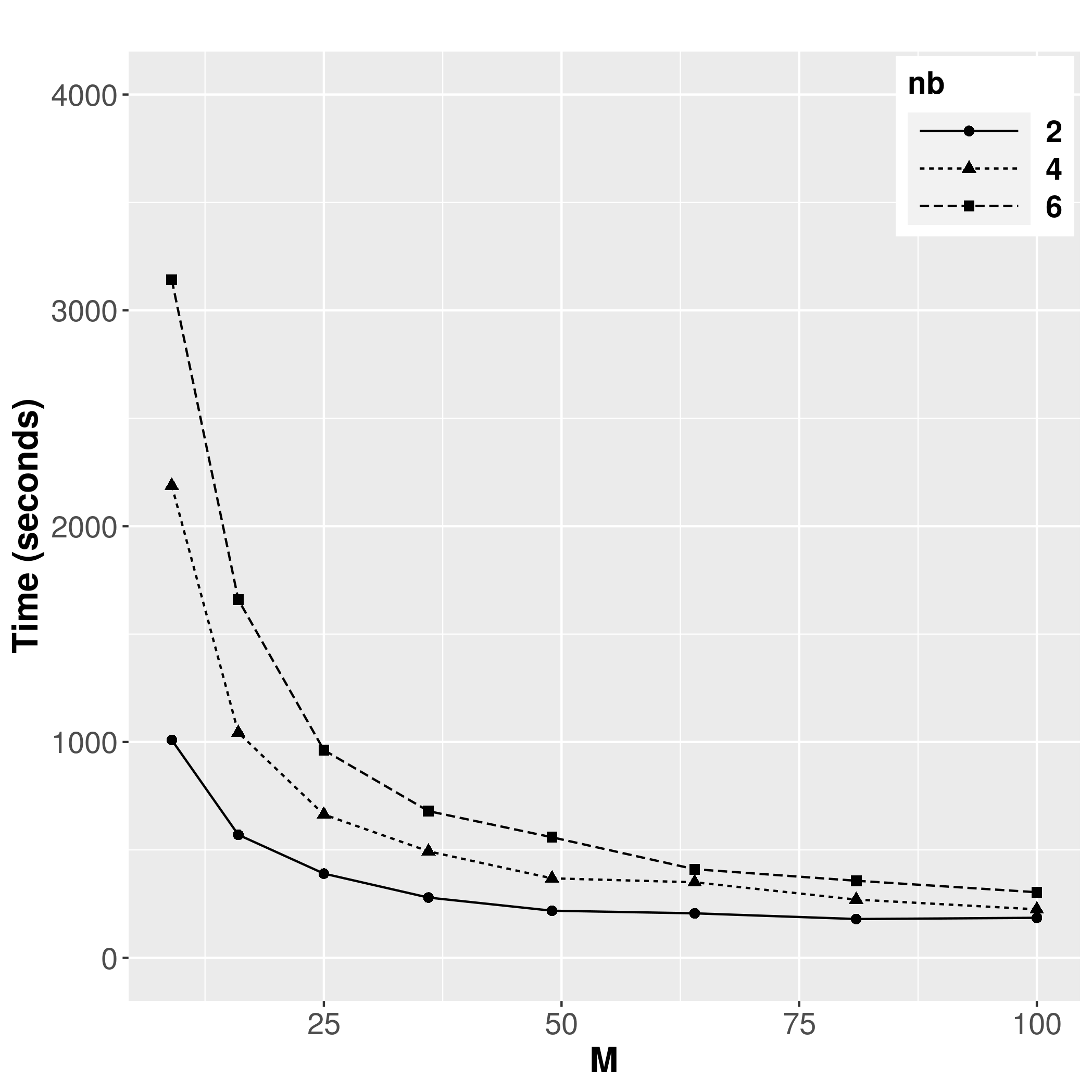
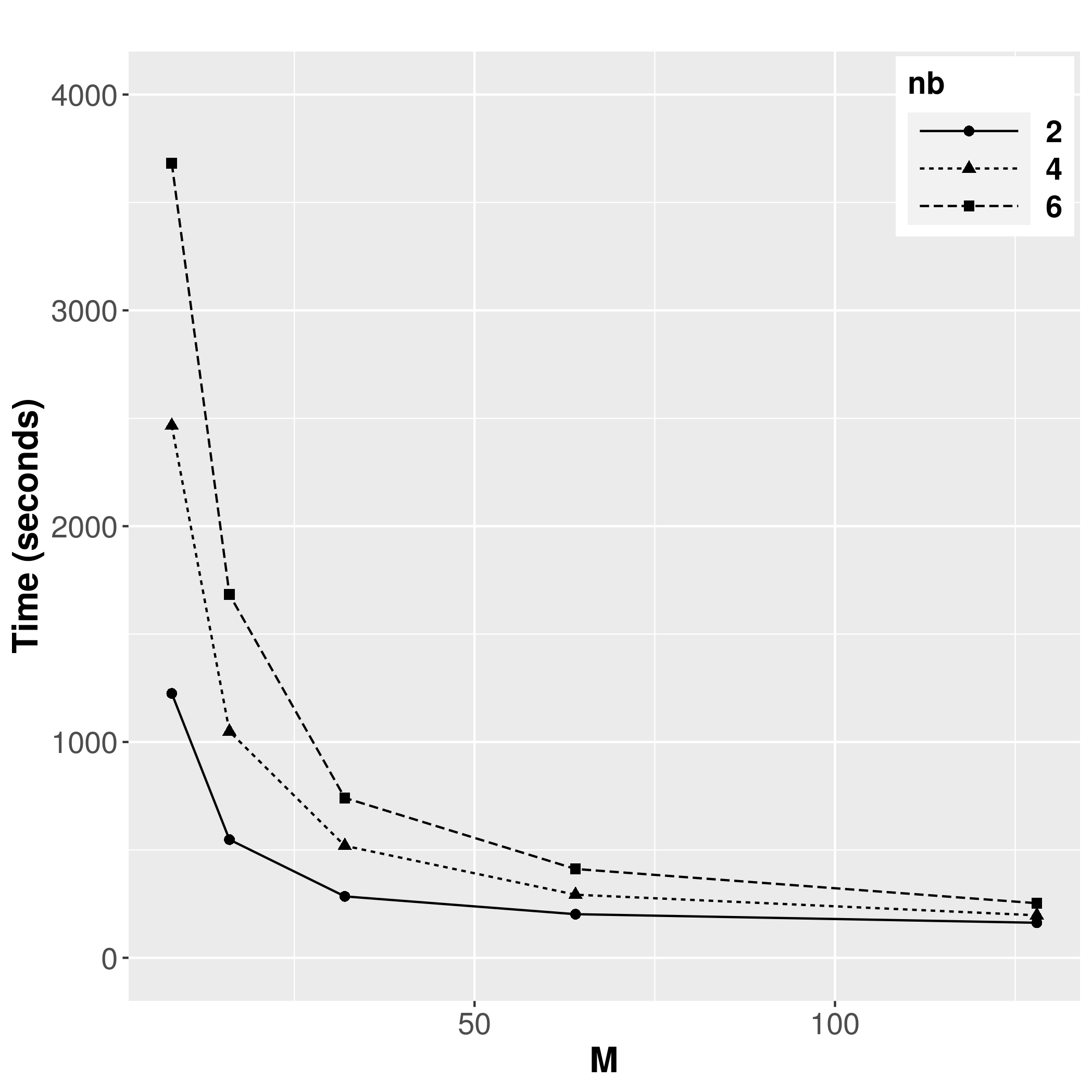
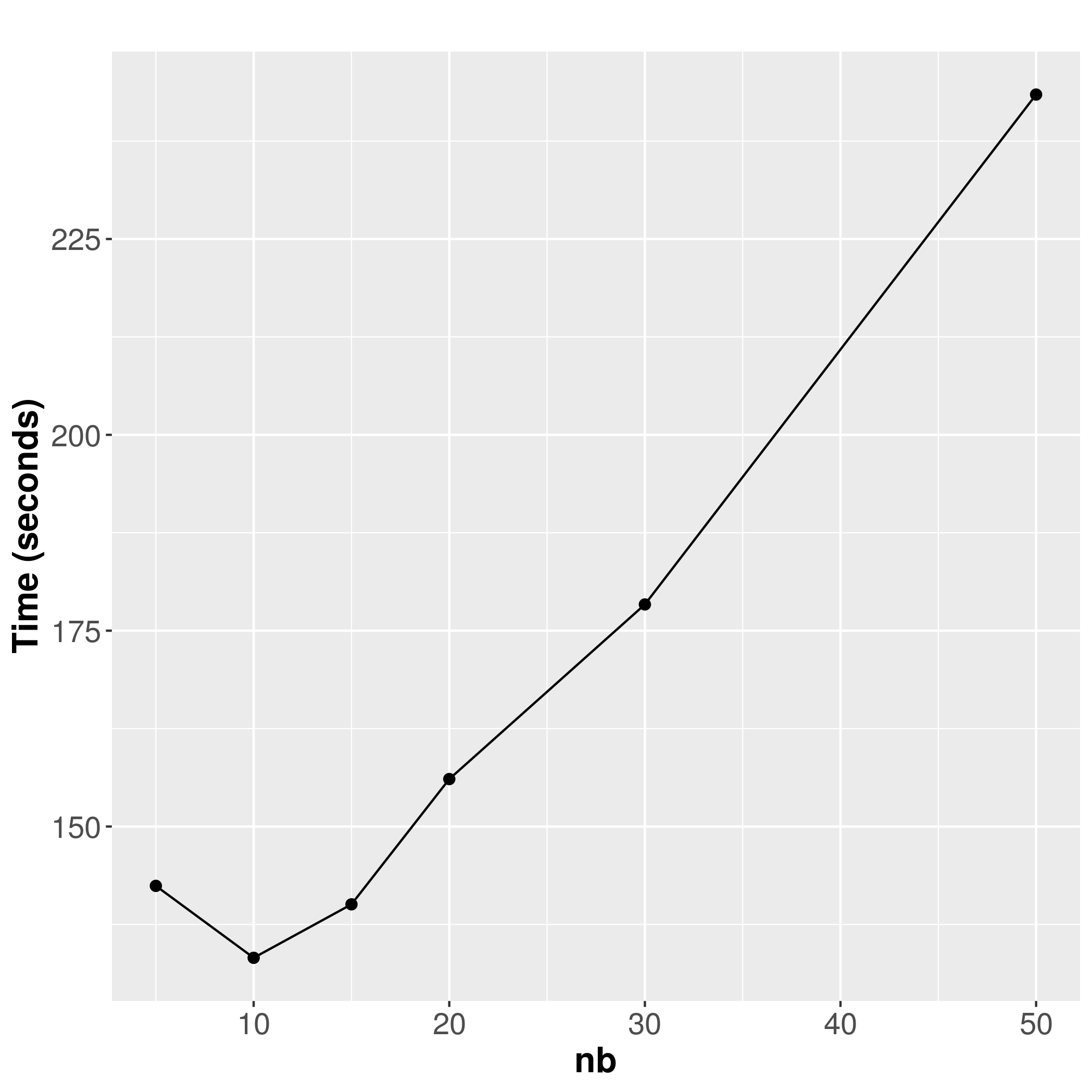
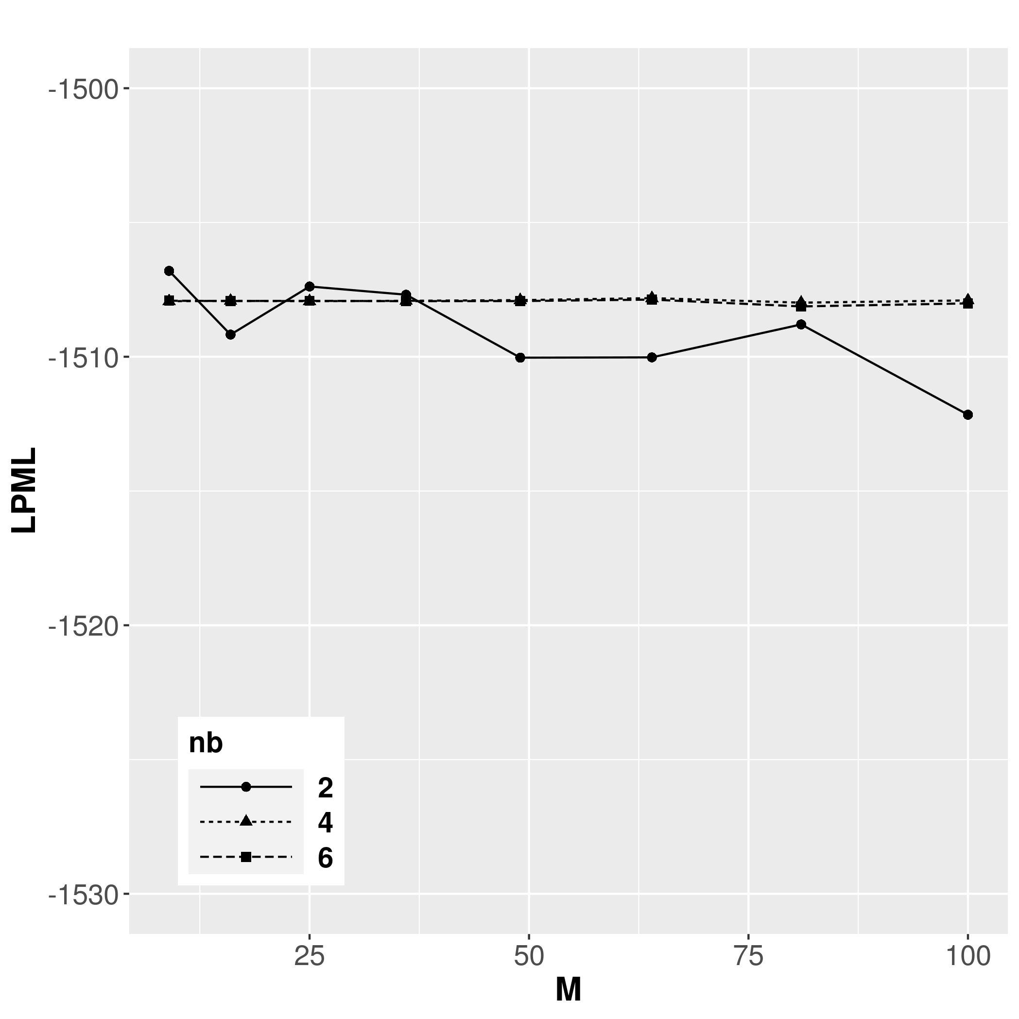
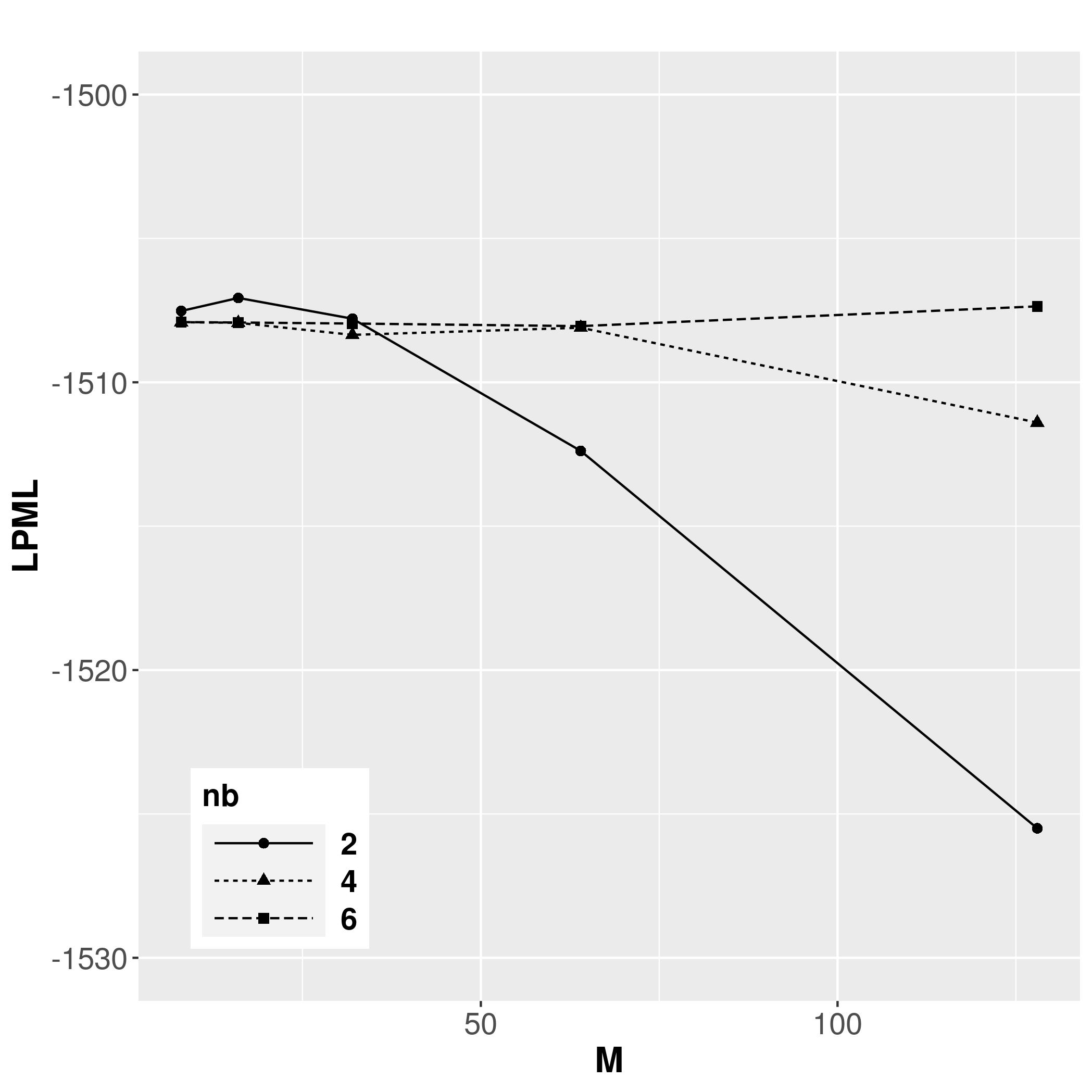
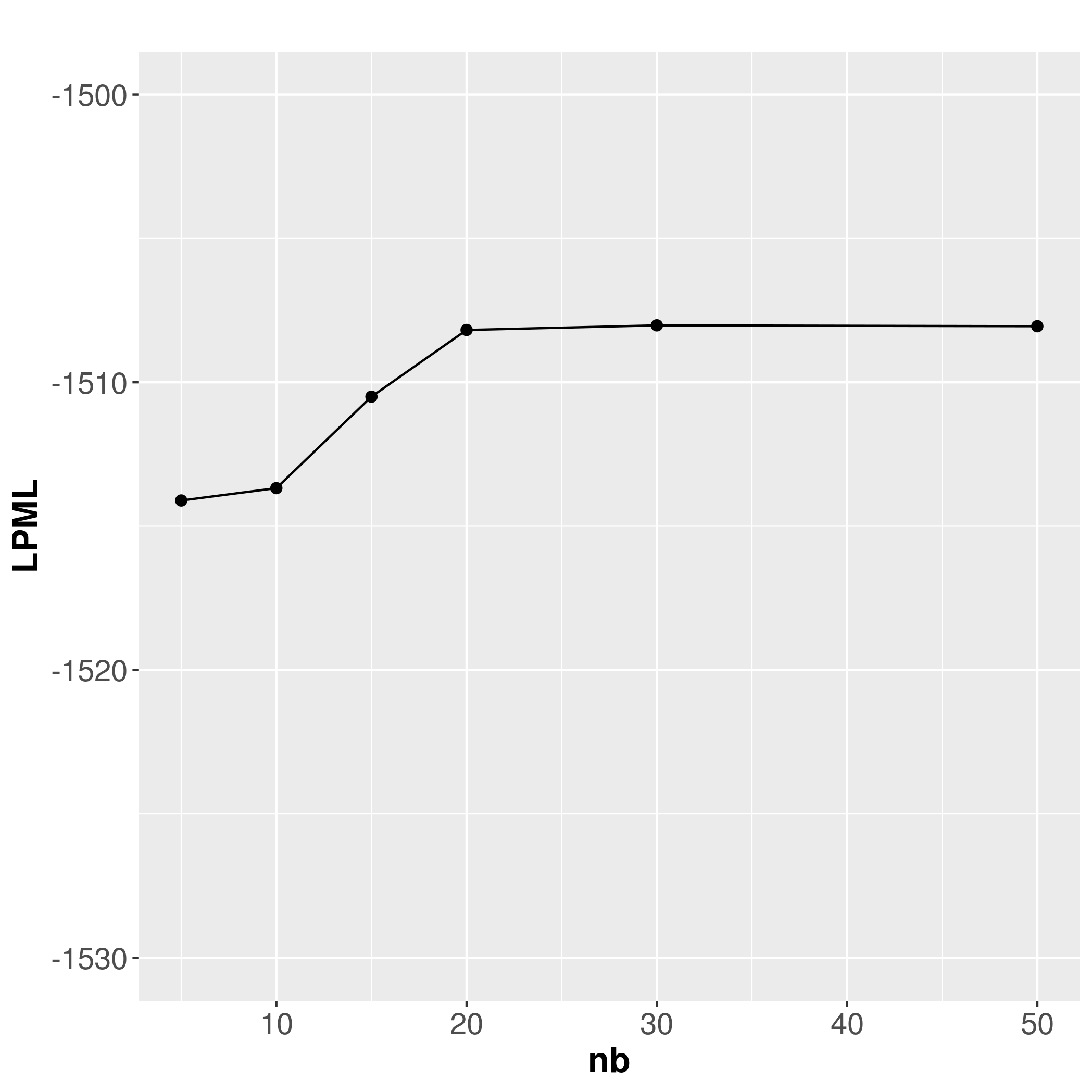
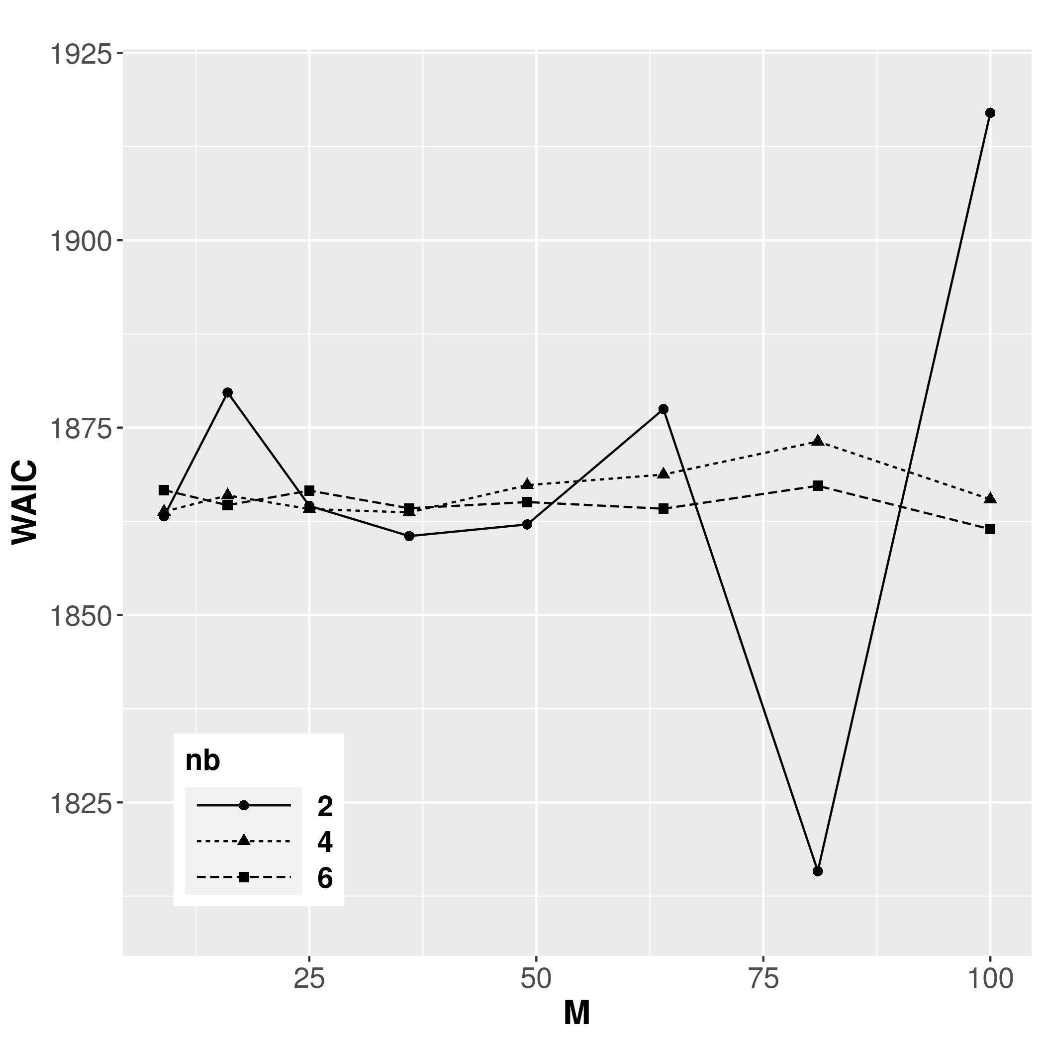
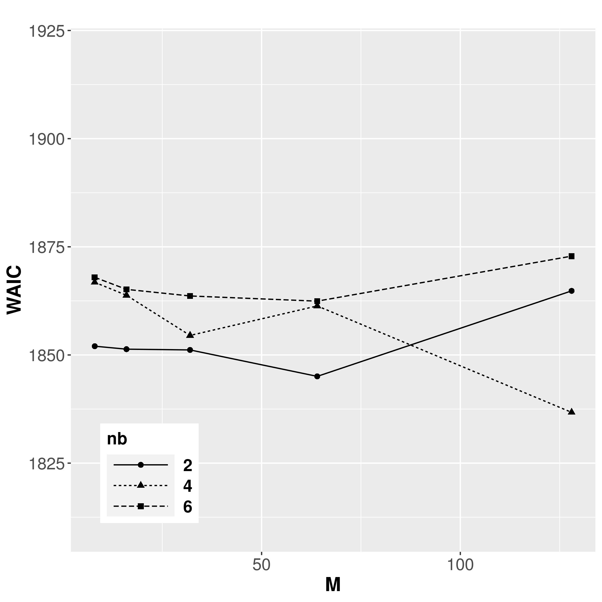
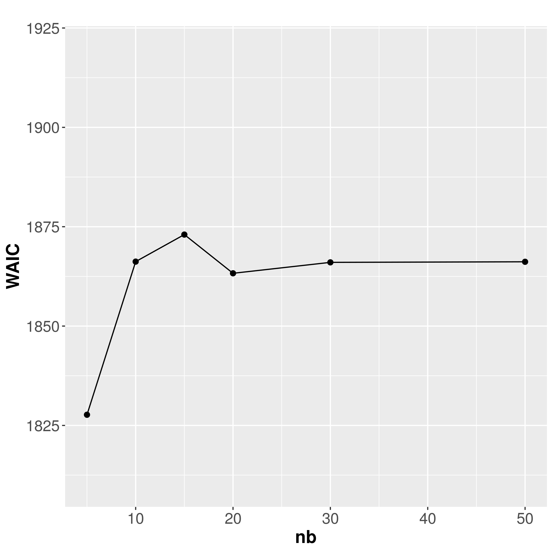
Figure S1: SIM I ($\phi$ = 12). INLA results. Criteria assessment: Running times (first row), LPML (second row) and WAIC (third row), under block-NNGP models using regular blocks (left column), irregular blocks (middle column) and NNGP models (right column).

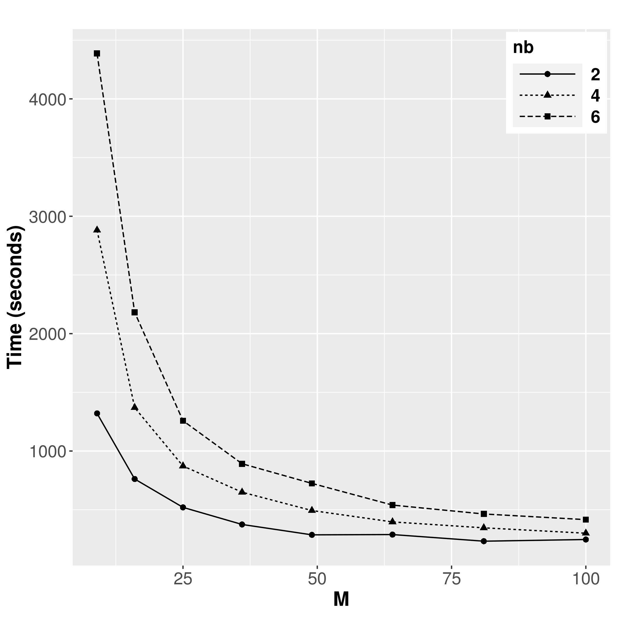
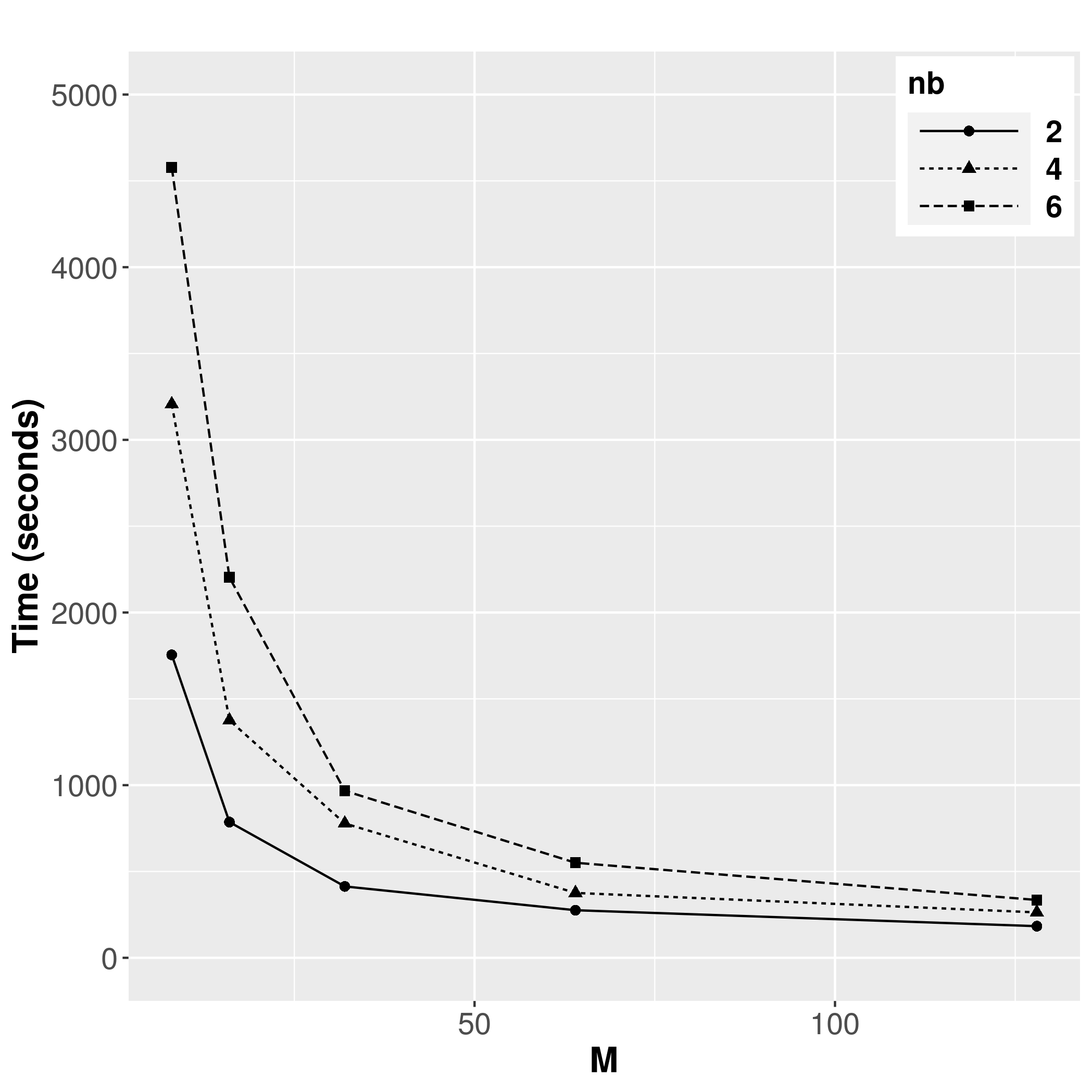
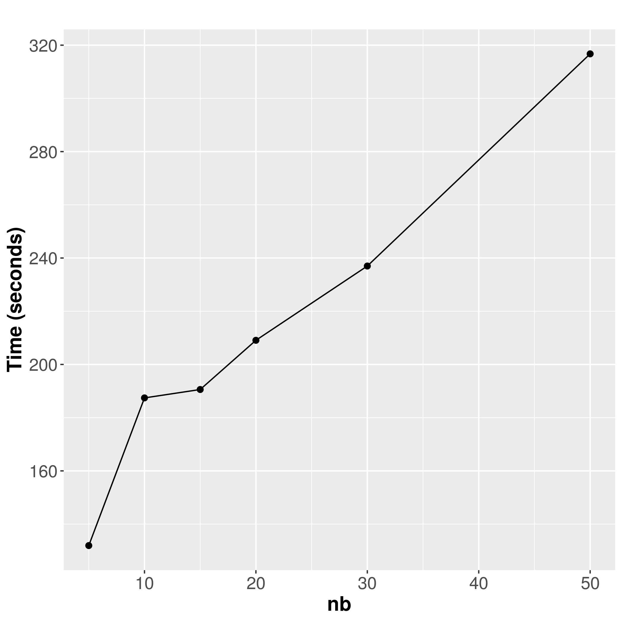
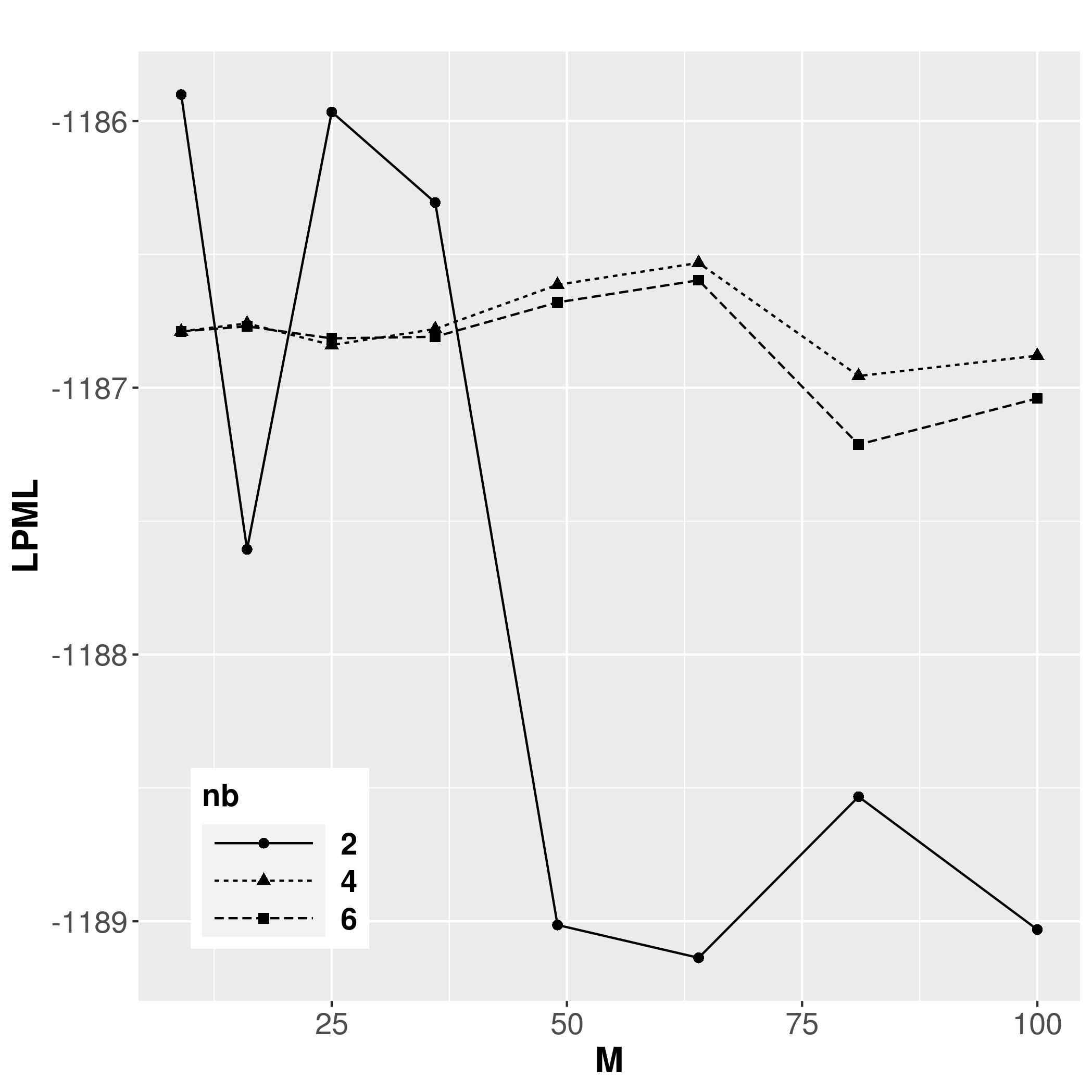
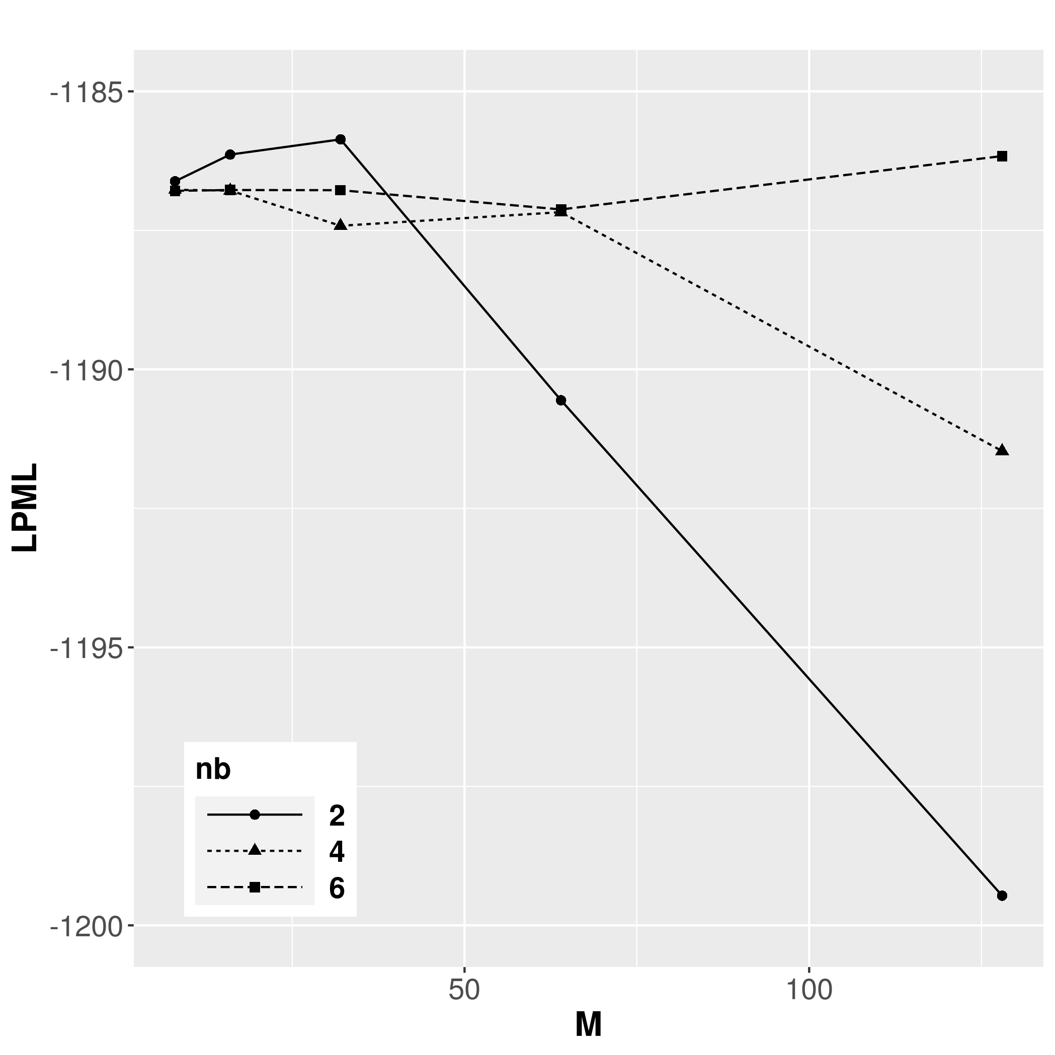
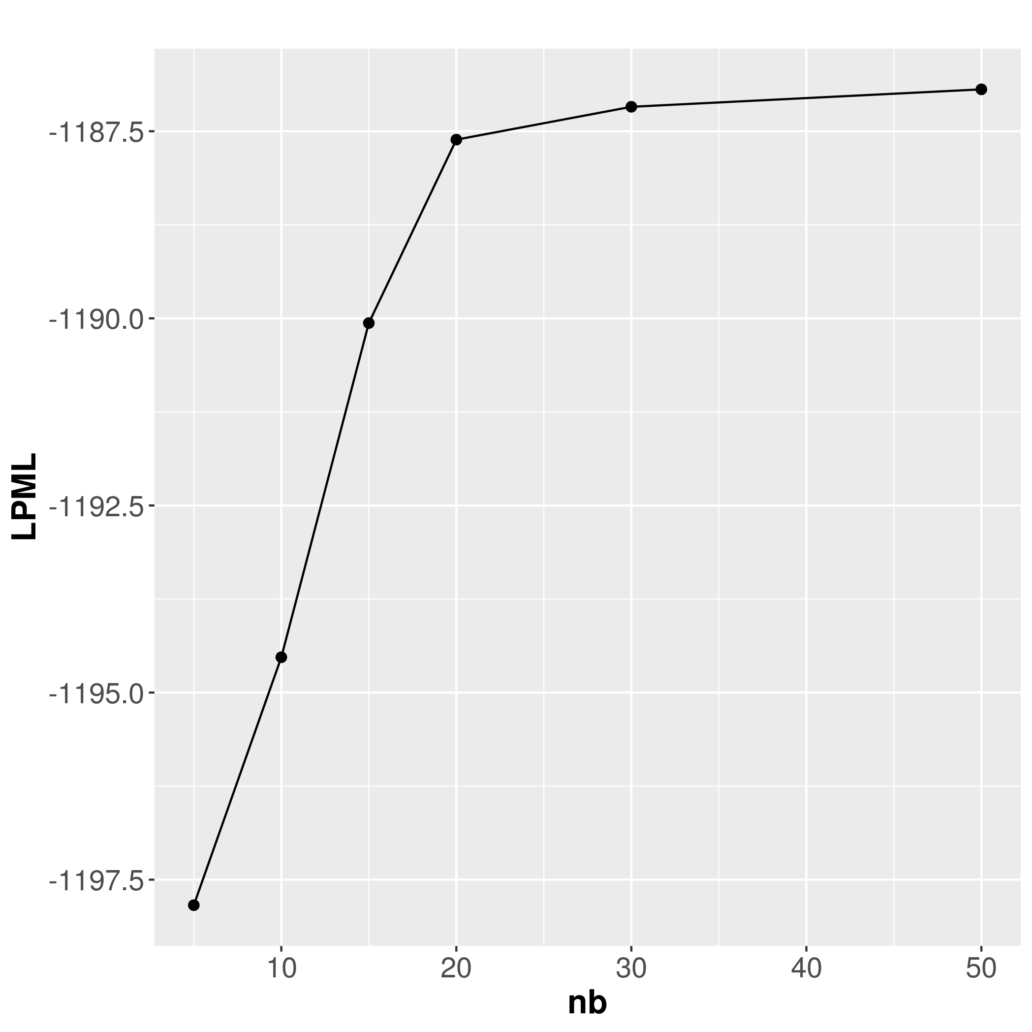
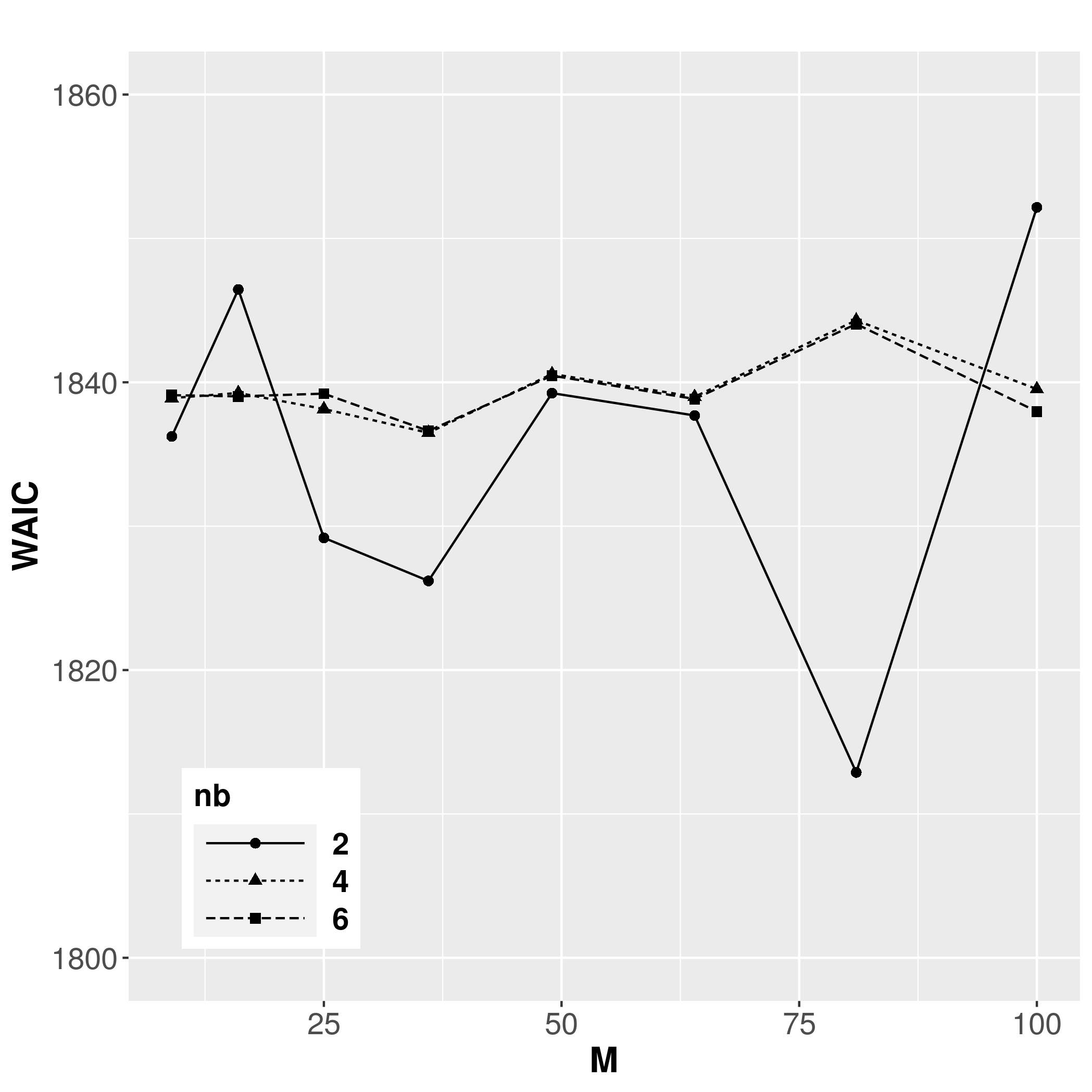
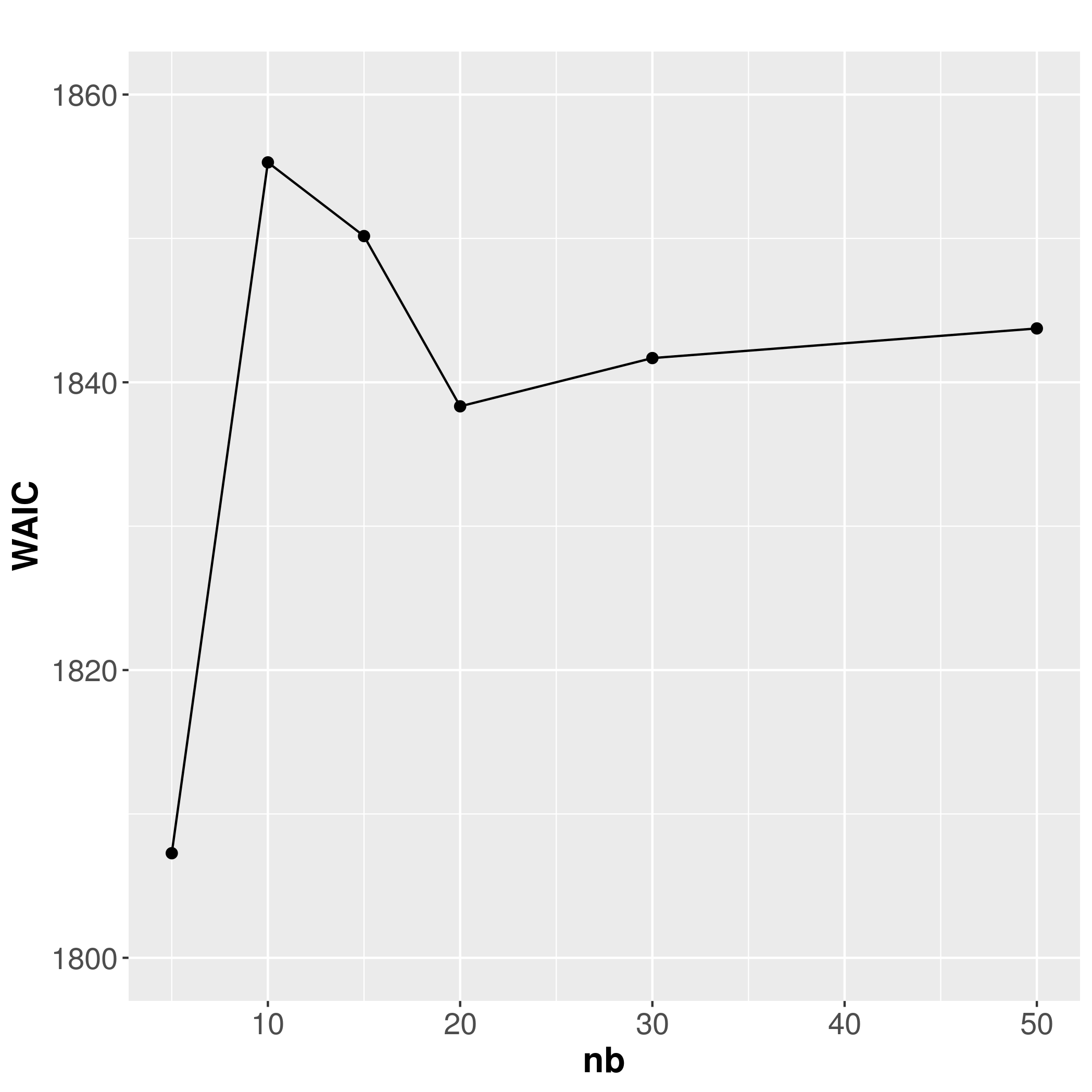
Figure S2: SIM II ($\phi$ = 6). INLA results. Criteria assessment: Running times (first row), LPML (second row) and WAIC (third row), under block-NNGP models using regular blocks (left column), irregular blocks (middle column) and NNGP models (right column).

Figure S3: SIM I ($\phi=12$). INLA results. Mean posterior estimates of spatial effects for different NNGP (upper panel) and block-NNGP models (lower panel).

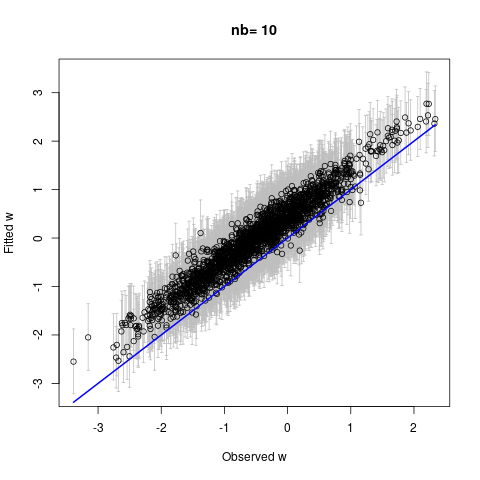
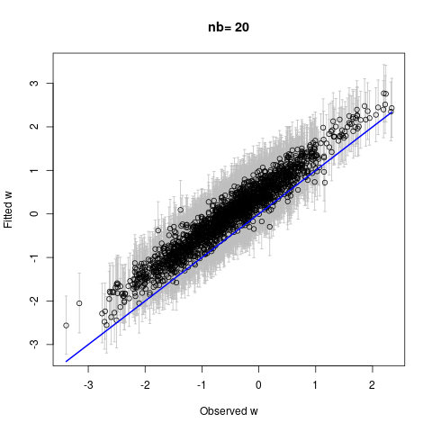
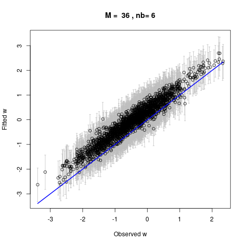
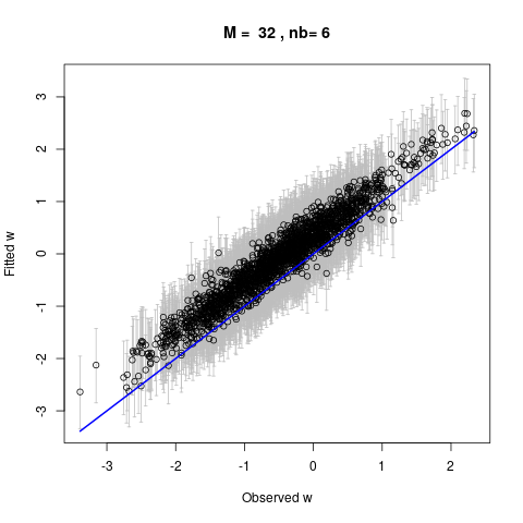
Figure S4: SIM II ($\phi=6$). INLA results. Mean posterior estimates of spatial effects for different NNGP (upper panel) and block-NNGP models (lower panel).

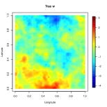
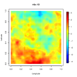
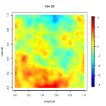
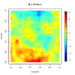
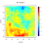
Figure S5: SIM III ($\phi$ = 3). True spatial random effects $w$, and their posterior mean estimates for NNGP models (upper panel) with $nb=10,20,30$ neighbors, and different block-NNGP models (lower panel) with regular blocks (R) and irregular blocks (I), using INLA.

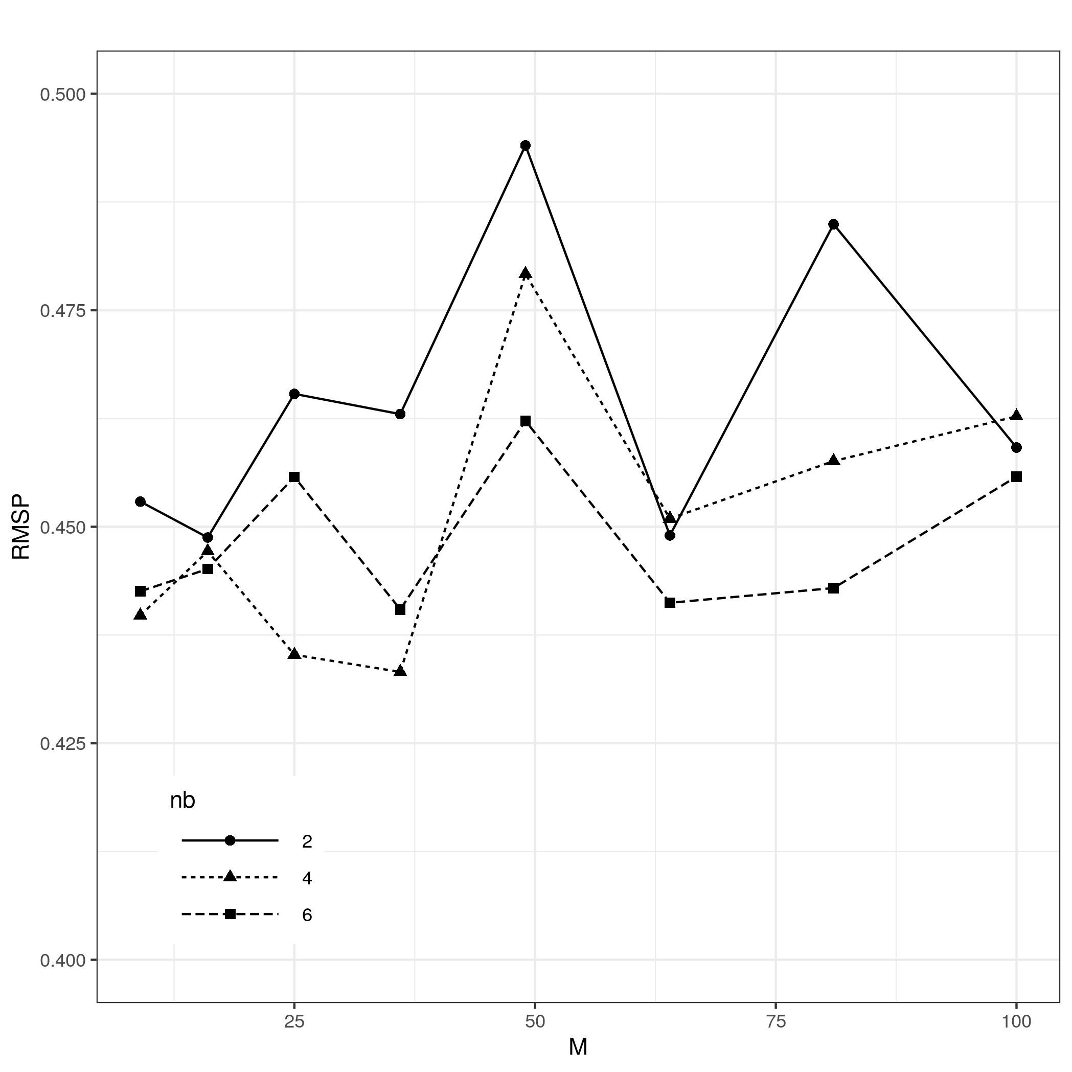
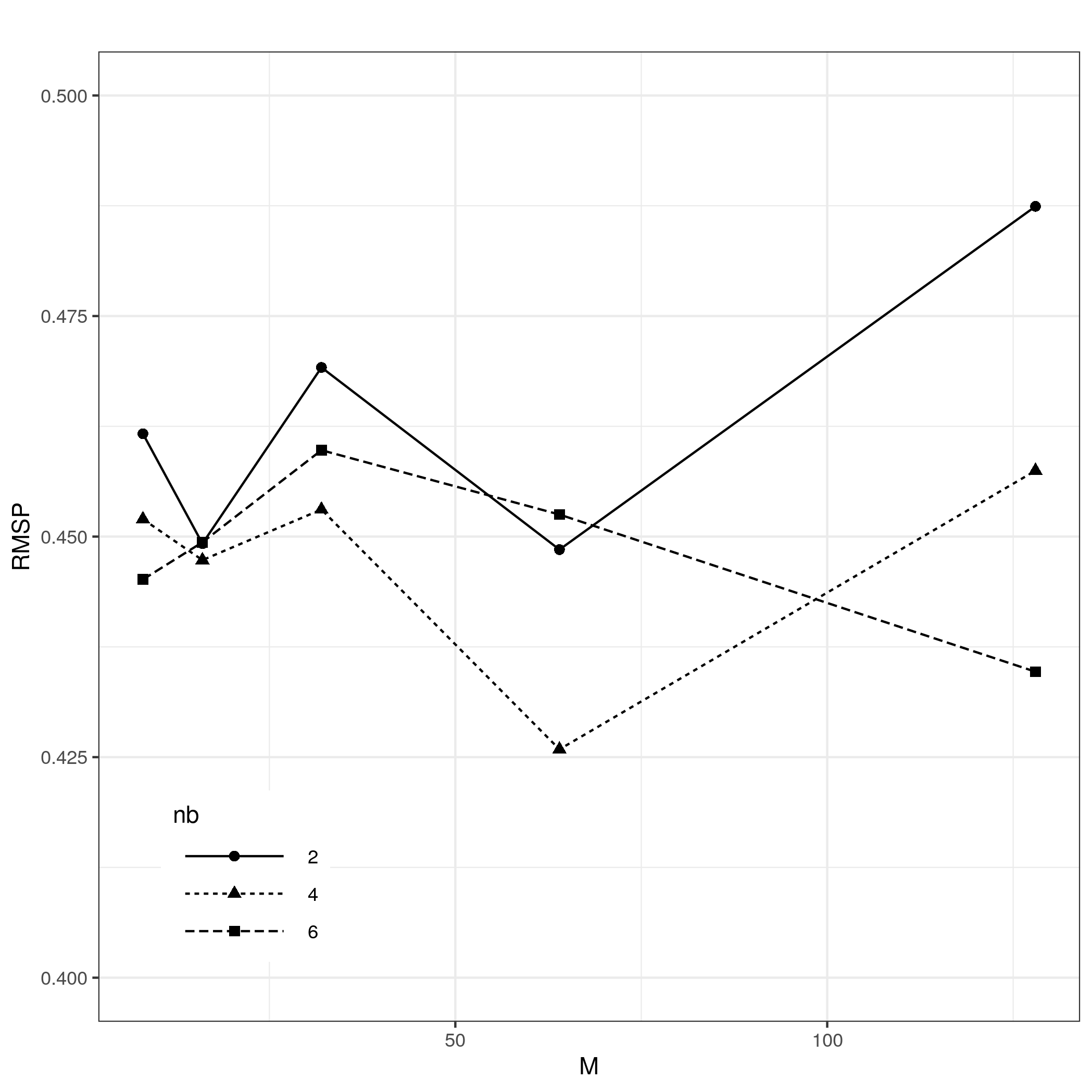
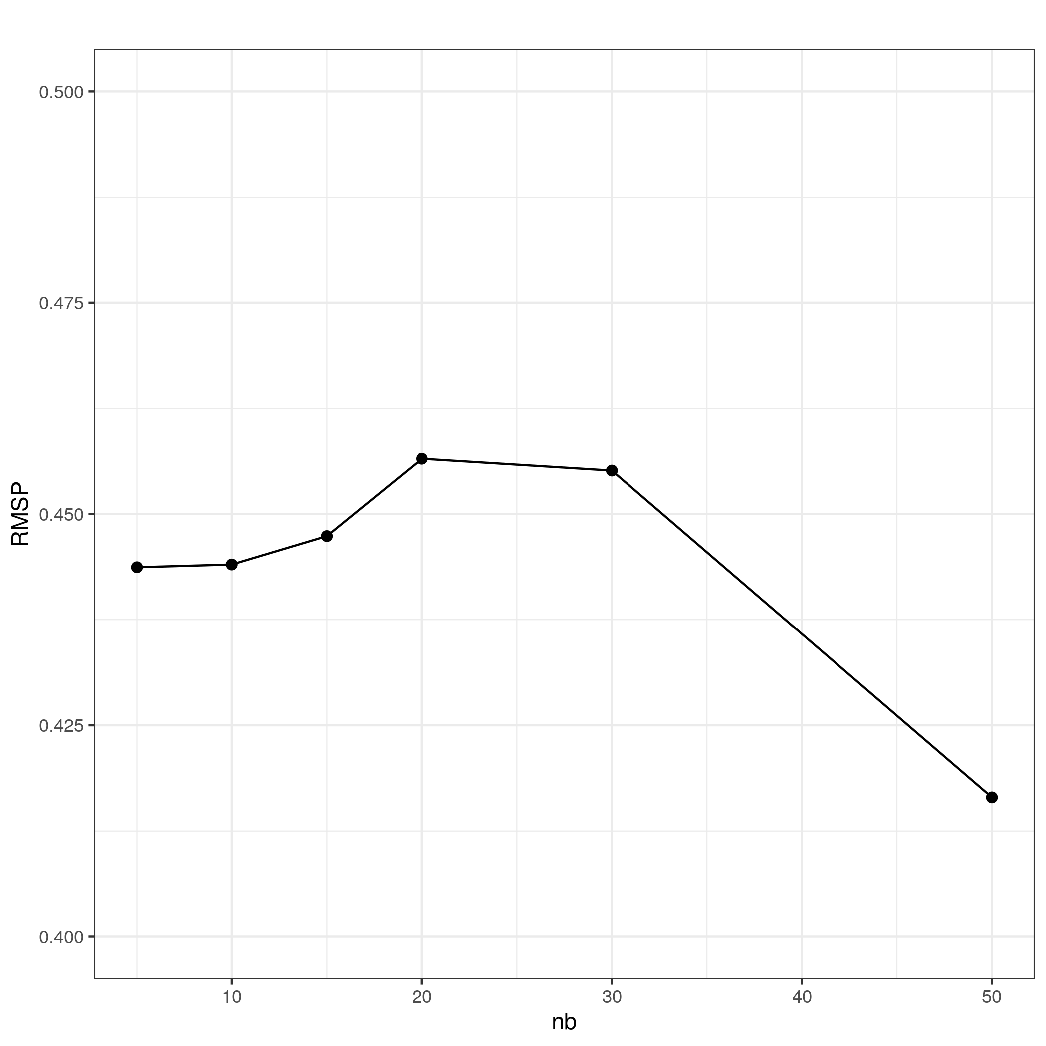
Figure S6: SIM III ($\phi$ = 3). INLA results. Root mean square prediction error under block-NNGP models using regular blocks (left column), irregular blocks (middle column) and NNGP models (right column).

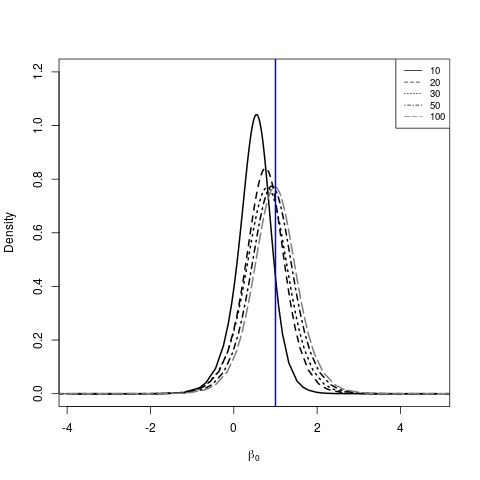
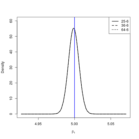
Figure S7: INLA results for simulation of GP with Matérn covariance function ($\nu=1.5$, $\phi=3.5$, $\sigma^{2}=1$ and $\tau^{2}=0.1$). Posterior marginal densities of regression coefficient effects for NNGP models (upper panel)with $nb=10,20,30,50,100$ neighbors and block-NNGP models (lower panel) with $M=25,36,64$ regular blocks and $nb=6$ neighbor blocks. The solid vertical blue lines represent the true parameter values.

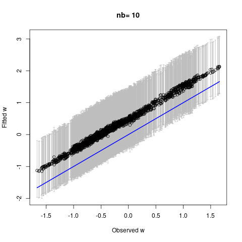
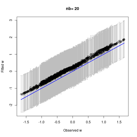
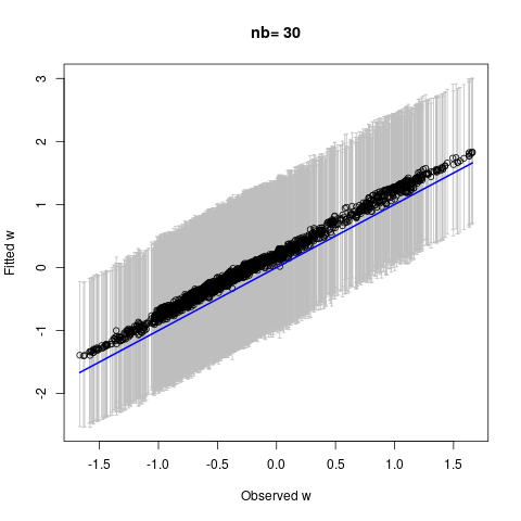
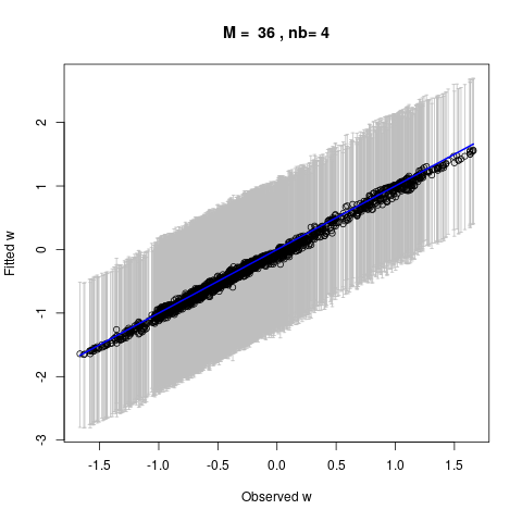
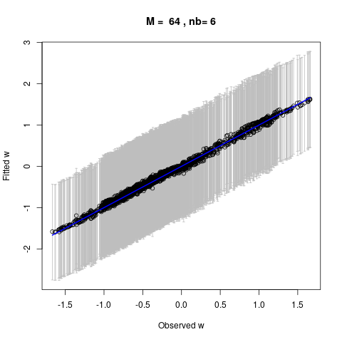
Figure S8: INLA results for simulation of GP with Matérn covariance function($\nu=1.5$, $\phi=3.5$, $\sigma^{2}=1$ and $\tau^{2}=0.1$). Mean posterior estimates of spatial effects for different NNGP (upper panel) and block-NNGP models using regular blocks (lower panel).

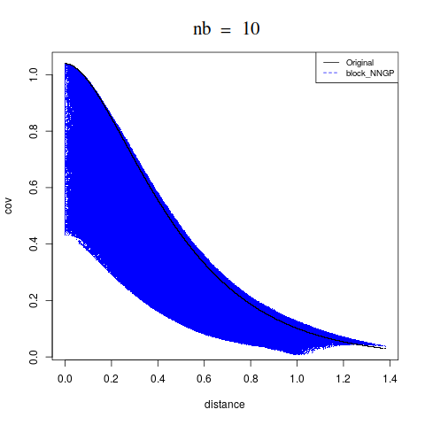
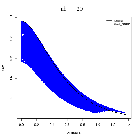
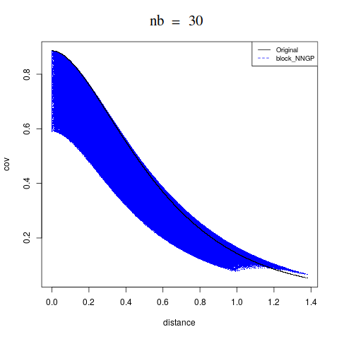
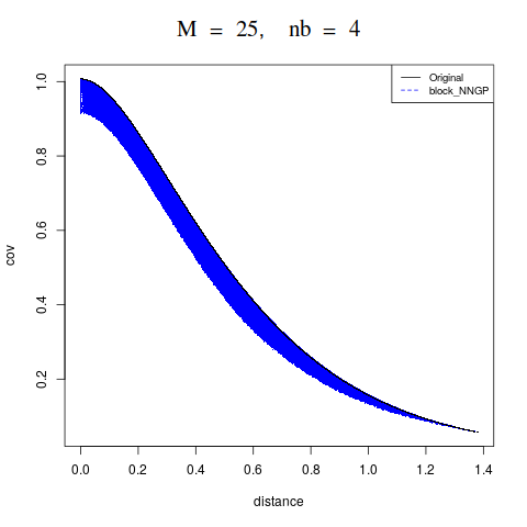
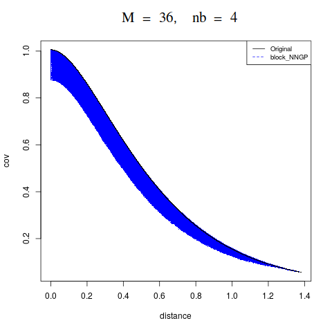
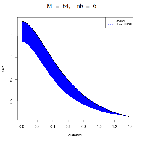
Figure S9: True Matérn covariance function ($\nu=1.5$, $\phi=3.5$, $\sigma^{2}=1$ and $\tau^{2}=0.1$) of GP against distance (black lines) and empirical approximated covariance of block-NNGP (Regular blocks) against distance (blue dots) for different NNGP (upper panel) and block-NNGP models (lower panel).

D. Supplementary application results

Fig. S10 shows an example of DAGs, built using one location for each block, for the mining and precipitation data used in applications. Figure S11 shows maps of interpolated posterior mean estimates of joint-frequency data. We see little difference between these models. Table S1 presents the selection criteria of the fitted models. This result shows that it is quite difficult to choose the number of neighbors, because there is not a clear pattern that the more neighbors, the better the model. While the best block-NNGP model is the one with $M=64$ and $nb=4$ neighbor blocks, followed by the model with $M=64$ and $nb=6$ neighbor blocks. Overall, the results are more stable for less blocks and more neighbor blocks. Table S1 also presents the total running time for each model.

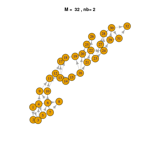
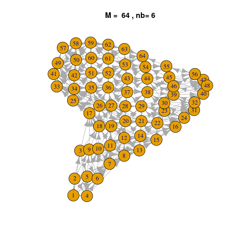
Figure S10: DAG of blocks for mining data (left) using 32 blocks and 2 neighbor blocks. DAG of blocks for precipitation data (right) using 64 blocks and 6 neighbor blocks.

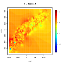
Figure S11: Original joint-frequency data (left upper plot). INLA results. Mean posterior of joint-frequency data using NNGP models with $nb=10,20$ neighbors (upper panel). Mean posterior of joint-frequency data using block-NNGP models with regular blocks (M=450 and M=280) and irregular blocks (M=128), and nb=1 neighbor block (lower panel).

Table S1: Precipitation data. INLA results. Criteria assessment and time requirements.

	M	nb	LPML	WAIC	RSME	RSMP	time (sec)
		10	-18407.420	-11705.390	0.0052	0.523	1535.664
		20	-18863.340	-11750.800	0.0051	0.467	2588.953
NNGP		30	-19167.690	-11666.300	0.0051	0.626	1356.085
		50	-19228.520	-11680.250	0.0051	0.561	1745.064
		100	-18875.250	-11783.170	0.0050	0.508	5019.320
	64	2	-19533.230	-11642.630	0.0050	0.598	7191.660
	64	4	-19141.680	-11736.000	0.0050	0.680	13587.350
block-NNGP (I)	64	6	-19436.940	-11708.210	0.0050	0.645	19992.250
	128	2	-19661.130	-11595.540	0.0049	0.645	2740.382
	128	4	-19483.990	-11625.660	0.0051	0.595	5434.684
	128	6	-19381.560	-11680.610	0.0050	0.742	5092.628

References

- Abrahamsen, (1997) Abrahamsen, P. (1997). A review of gaussian random fields and correlation functions. Technical report.
- Banerjee, (2020) Banerjee, S. (2020). Modeling massive spatial datasets using a conjugate bayesian linear modeling framework. Spatial Statistics, 37:100417. Frontiers in Spatial and Spatio-temporal Research.
- Banerjee et al., (2008) Banerjee, S., Gelfand, A. E., Finley, A. O., and Sang, H. (2008). Gaussian predictive process models for large spatial datasets. Journal of the Royal Statistical Society, Series B, 70:825–848.
- Bentley, (1975) Bentley, J. L. (1975). Multidimensional binary search trees used for associative searching. Commun. ACM, 18(9):509–517.
- Bolin and Wallin, (2016) Bolin, D. and Wallin, J. (2016). Spatially adaptive covariance tapering. Spatial Statistics, 18(Part A):163 – 178.
- Calaway et al., (2017) Calaway, R., Analytics, R., and Weston, S. (2017). doMC: Foreach Parallel Adaptor for ”parallel”.
- Caragea and Smith, (2007) Caragea, P. C. and Smith, R. L. (2007). Approximate likelihoods for spatial processes. In Joint Statistical Meetings - Section on Statistics & the Environment.
- Cressie, (1993) Cressie, N. (1993). Statistics for Spatial Data. Wiley Classics Library.
- Datta et al., (2016) Datta, A., Banerjee, S., Finley, A. O., and Gelfand, A. E. (2016). Hierarchical nearest-neighbor Gaussian process models for large geostatistical datasets. Journal of the American Statistical Association, 111(514):800–812.
- Diggle et al., (1998) Diggle, P. J., Tawn, J. A., and Moyeed, R. A. (1998). Model-based geostatistics. Journal of the Royal Statistical Society: Series C (Applied Statistics), 47(3):299–350.
- Eidsvik et al., (2014) Eidsvik, J., Shaby, B. A., Reich, B. J., Wheeler, M., and Niemi, J. (2014). Estimation and prediction in spatial models with block composite likelihoods. Journal of Computational and Graphical Statistics, 23(2):295–315.
- Finley et al., (2019) Finley, A. O., Datta, A., Cook, B. D., Morton, D. C., Andersen, H. E., and Banerjee, S. (2019). Efficient algorithms for bayesian nearest neighbor gaussian processes. Journal of Computational and Graphical Statistics, 28(2):401–414. PMID: 31543693.
- Guinness, (2018) Guinness, J. (2018). Permutation and grouping methods for sharpening gaussian process approximations. Technometrics, 60(4):415–429.
- Kaufman et al., (2008) Kaufman, C. G., Schervish, M. J., and Nychka, D. W. (2008). Covariance tapering for likelihood-based estimation in large spatial data sets. Journal of the American Statistical Association, 103(484):1545–1555.
- Kaufman and Shaby, (2013) Kaufman, C. G. and Shaby, B. A. (2013). The role of the range parameter for estimation and prediction in geostatistics. Biometrika, 100(2):473–484.
- Lee and Haran, (2019) Lee, B. S. and Haran, M. (2019). Picar: An efficient extendable approach for fitting hierarchical spatial models. arXiv preprint arXiv:1912.02382.
- Lindgren et al., (2011) Lindgren, F., Rue, H., and Lindström, J. (2011). An explicit link between Gaussian fields and Gaussian Markov random fields: The SPDE approach. Journal of the Royal Statistical Society. Series B. Statistical Methodology, 73(4):423–498.
- Liu, (1994) Liu, J. S. (1994). The collapsed gibbs sampler in bayesian computations with applications to a gene regulation problem. Journal of the American Statistical Association, 89(427):958–966.
- Rue et al., (2009) Rue, H., Martino, S., and Chopin, N. (2009). Approximate bayesian inference for latent Gaussian models by using integrated nested Laplace approximations. Journal of the Royal Statistical Society B, 71(2):319–392.
- Rue and Tjelmeland, (2002) Rue, H. and Tjelmeland, H. (2002). Fitting Gaussian Markov random fields to Gaussian fields. Scandinavian Journal of Statistics, 29((1)):31–50.
- Stein, (2013) Stein, M. L. (2013). Statistical properties of covariance tapers. Journal of Computational and Graphical Statistics, 22(4):866–885.
- Stein et al., (2004) Stein, M. L., Chi, Z., and J.Welty, L. (2004). Approximating likelihoods for large spatial data sets. Journal of the Royal Statistical Society, Series B, 66(2):275–296.
- Whittle, (1954) Whittle, P. (1954). On stationary processes in the plane. Biometrika, 44:434–449.