Hybrid Deep Network for Anomaly Detection

Abstract

In this paper, we propose a deep convolutional neural network (CNN) for anomaly detection in surveillance videos. The model is adapted from a typical auto-encoder working on video patches under the perspective of sparse combination learning. Our CNN focuses on (unsupervisedly) learning common characteristics of normal events with the emphasis of their spatial locations (by supervised losses). To our knowledge, this is the first work that directly adapts the patch position as the target of a classification sub-network. The model is capable to provide a score of anomaly assessment for each video frame. Our experiments were performed on 4 benchmark datasets with various anomalous events and the obtained results were competitive with state-of-the-art studies.

1 Introduction

Anomaly detection in surveillance videos is currently getting attention for the development of automatic vision systems. Since anomalous events rarely happen in a long video, a method that can determine the potential of such events at frame-level is necessary.

Many approaches have been proposed to deal with this problem by processing either entire video frames [Li et al. (2014), Zhang et al. (2016), Hasan et al. (2016), Liu et al. (2018)] or small image patches [Kim and Grauman (2009), Zhao et al. (2011), Cheng et al. (2015), Xu et al. (2015), Luo et al. (2017)]. Our work is inspired by the study [Lu et al. (2013)] belonging to the latter category. Specifically, Lu et al. (2013) partition the image plane into non-overlapping regions and then concatenate a number of successive frames to obtain spatio-temporal cuboids. The sparse combination learning is applied on such cuboids of the same spatial position. In other words, the anomaly assessment is performed independently on each region of input frames.

Following the spectacular development of deep CNNs in various vision problems such as image classification Krizhevsky et al. (2012); He et al. (2016) and object detection Ren et al. (2015); He et al. (2017), we attempt to replace the sparse combination learning applied for each spatial region by a convolutional auto-encoder (AE). The former algorithm focuses on representing an unknown input as a weighted combination of training samples while the latter one emphasizes their common characteristics. A trivial replacement leads to the use of a number of AEs where each one is assigned to a specific image patch position. Such ensemble of AEs requires huge resources such as memory for execution and storage capacity for storing the model parameters. In order to avoid these problems, we adaptively combine all AEs into a single one by adding a classification sub-network that forces the emphasized features to contain the information related to their corresponding spatial location. To the best of our knowledge, this is the first study adapting image patch positions as the classes in a supervised task.

The main contributions of this paper are summarized as: (1) integrating a classification sub-network into a convolutional AE model as a constraint of feature learning, (2) demonstrating that the combination of unsupervised and supervised objective functions provides better results than using only supervised learning for our anomaly detection, (3) a scheme combining scores obtained from different network components for improving the final anomaly assessment score, (4) experimental results on 4 benchmark datasets validating the competitive performance of the proposed model compared with state-of-the-art methods, and (5) a discussion regarding to the impact of the decoder in our hybrid network.

2 Related Works

One significant challenge of anomaly detection in surveillance videos is the diversity of anomalous events. In order to simplify this task, some studies (such as Medioni et al. (2001); Zhang et al. (2009); Bensch et al. (2015)) focus on one of common basic factors: motion trajectory. By estimating that feature in videos, the original task becomes a typical problem of novelty detection. Such approaches can be easy to implement and have a fast execution speed. However, considering only motion trajectory does not cover the high diversity of possible anomalies. Besides, a failure in object localization and/or tracking would significantly reduce the efficiency of anomaly detection.

Another popular method is the use of sparse coding where the training data (containing only normal events) are a collection of small pieces (e.g. image patches, 3D cuboids and/or their features) and a new input is then represented as a combination of training patterns. A normal event is expected to provide a reconstructed combination result with small error and vice versa. These methodologies have reported to give efficient performance in many studies Kim and Grauman (2009); Zhao et al. (2011); Lu et al. (2013). A drawback of most approaches with this perspective is the high computational cost during the stage of searching sparse combination.

Recent studies employ deep neural networks with various architectures to perform image reconstruction Hasan et al. (2016) and/or translation Ravanbakhsh et al. (2017, 2019) and use the estimated loss as the measure of normality in video frames. These methods can be applied on the whole frames Liu et al. (2018); Hasan et al. (2016) or image patches Xu et al. (2017); Sabokrou et al. (2018). Our model also falls into this category but integrates a classification sub-network to adapt the perspective of the work Lu et al. (2013) belonging to the previous one. Our hybrid network is expected to take advantages from both categories.

3 Hybrid Deep Network

As mentioned in the previous section, the hybrid model consists of two principal streams. The first one is a typical AE focusing on emphasizing common features of normal events at patch-level. The second stream performs a classification on the extracted characteristics and can be considered as a constraint for the former stream. Similarly to Lu et al. (2013), we work on 3D cuboid of small spatial resolution of frame concatenation, in which these frames are resized to $160\times 120$ and are gray-scale. However, we consider only 3 successive frames instead of 5 as in that study for faster execution without significant performance loss. The input of our model is thus a cuboid of size $10\times 10\times 3$. An overall architecture of the hybrid network is presented in Fig. 1(a). More details can be found in the supplementary material.

Figure 1: (a) Our hybrid network where input is a cuboid of size $10\times 10\times 3$. Data transfer indicates that the output of a layer is used by multiple next ones. The spatial dimensions of feature maps in each block are provided together with their number of channels (in parentheses). Notice that there are usually 2 numbers of channels because of the second convolutional layer (colorized as yellow). (b) The discriminator used for adversarial training in Section 3.3.3. Best viewed in color.

3.1 Convolutional auto-encoder for learning common features

The AE in our hybrid network aims to learn common local features of normal events. It works as a reconstruction model with a bottleneck structure. The temporal factor is embedded into this learning by concatenating consecutive frames. Some studies (e.g. Xu et al. (2015); Liu et al. (2018)) instead employ optical flow to represent this information. Such estimators may produce noisy results and/or require a training stage, e.g. FlowNet Dosovitskiy et al. (2015) and its upgraded version Ilg et al. (2017).

As visualized in Fig. 1(a), there are two main components in our AE. The encoder is formed as a stack of layer blocks that reduce the resolution of feature maps, in which each block consists of two convolutional (Conv) layers, batch normalization, and activation. The first Conv layer converts the spatial dimensions of its input and the second one then transforms the features to a specific number of channels. Although these two operations can be performed with only one Conv layer, recent studies demonstrated good efficiencies when using this trick Liu et al. (2018). The use of the first Conv layer can be considered as an alternative to the pooling operation. In the decoder, this layer is replaced by deconvolution to upscale the spatial dimensions. Besides, the dropout (with probability set as 0.5) is integrated right before the activation layer. Notice that there is no batch normalization in the first block of the encoder and we use different activations for the two components (leakyReLU Maas et al. (2013) for the encoder and ReLU Nair and Hinton (2010) for the decoder) as suggested in Isola et al. (2017) although the skip connection is not employed in our model. The last layer of the decoder is a Conv layer that transforms the reconstructed features into the original size of $10\times 10\times 3$.

3.2 Classification sub-network

Besides learning common local features in cuboids of normal events by the AE, we also add a constraint to the encoder so that the extracted information reveals spatial locations. To do that, the outputs of encoder blocks are vectorized and then concatenated to give a feature vector of 7104 elements. Notice that a convolution of $1\times 1$ filters is performed before the vectorization to reduce the number of channels except for the latent variables [see Fig. 1(a)].

Since each frame of size $160\times 120$ is partitioned into non-overlapping $10\times 10$ patches, there are a total of $16\times 12=192$ possible locations for an input cuboid. A classification problem with 192 classes on such small cuboid may be too complicated. In order to simplify this task, each patch position is represented by its spatial dimensions. Therefore, the classification is performed on two branches predicting the horizontal and vertical indices of image patches. The total number of classes is hence reduced to $16+12=28$. In addition, such architecture also allows the model to learn common features of cuboids belonging to the same row and the same column. This sub-network is a stack of dense layers with ReLU activation followed by a dropout, and the final outputs are provided by a softmax layer.

3.3 Model optimization

The optimization of our hybrid network is performed according to the objective functions of its partial components: reconstruction loss for the AE, classification loss for the location prediction sub-network, and adversarial training as an enhancement for reconstruction.

3.3.1 Reconstruction loss

This loss is defined as the difference between an input cuboid and its reconstructed result. In this work, we use the typical $l_{2}$ distance to measure this factor. A drawback of $l_{2}$ distance is the blur occurring in the obtained cuboid. To reduce this effect, an additional constraint on image spatial gradients is added into the objective function. This regularization improved the results provided by the decoder as reported in Mathieu et al. (2015); Liu et al. (2018). Since the input cuboid is formed with the concatenation of successive image patches in temporal order, we also consider the gradient along this axis as a constraint related to the local motion. Given an input cuboid $\mathbf{c}$ and a convolutional auto-encoder $\mathcal{M}$, the final reconstruction loss is a combination of mentioned losses in an unsupervised learning way as

$$\mathcal{L}_{R}(\mathbf{c},\mathcal{M})=\lambda_{l_{2}}\big{\|}\mathbf{c}-\mathcal{M}(\mathbf{c})\big{\|}^{2}_{2}+\lambda_{\nabla}\sum_{d\in\{x,y,t\}}\big{\|}|\nabla_{d}(\mathbf{c})|-|\nabla_{d}(\mathcal{M}(\mathbf{c}))|\big{\|}_{1}$$ (1)

where $\lambda$s are the positive weights controlling the contribution of partial losses while $x$, $y$ and $t$ respectively indicate the cuboid’s spatial and temporal dimensions. Notice that the gradient constraint is used in our objective function according to its efficiency in deep networks for reconstruction and frame prediction while 3D gradients are also employed in Lu et al. (2013) for feature description.

3.3.2 Classification loss

As mentioned above, the classification sub-network is to force learned common features to characterize cuboid spatial locations. The corresponding loss is computed as the summation of two dimensional predictions. Let $\mathcal{P}_{x}(\mathbf{c},l_{x})$ and $\mathcal{P}_{y}(\mathbf{c},l_{y})$ be the posterior probabilities of class labels $l_{x}$ and $l_{y}$ for the two classifiers given a cuboid $\mathbf{c}$ at position $(\mathbf{c}_{x},\mathbf{c}_{y})$, our classification loss is defined as the summation of cross-entropies as

$$\mathcal{L}_{C}(\mathbf{c})=-\sum_{l_{x}}\mathrm{I}(l_{x},\mathbf{c}_{x})\log\big{[}\mathcal{P}_{x}(\mathbf{c},l_{x})\big{]}-\sum_{l_{y}}\mathrm{I}(l_{y},\mathbf{c}_{y})\log\big{[}\mathcal{P}_{y}(\mathbf{c},l_{y})]$$ (2)

where $\mathrm{I}(\cdot,\cdot)$ returns 1 if the two operands are identical and 0 otherwise. There are a total of 16 labels for $l_{x}$ and 12 for $l_{y}$ corresponding to the classes along the horizontal and vertical dimensions since the resolution of input frames is $160\times 120$ with patch size of $10\times 10$.

3.3.3 Adversarial training

Besides the two mentioned losses, another term is added into the objective function as an attempt to enhance the quality of reconstructed cuboids. Specifically, we design an additional discriminative model to form a generative adversarial network (GAN) Goodfellow et al. (2014). A GAN includes a generator $\mathcal{G}$ that outputs desired data and a discriminator $\mathcal{D}$ which is a binary classifier attempting to distinguish such data with real patterns in training set. In other words, the two GAN components focus on opposite purposes in a game theory manner: $\mathcal{G}$ tries to fool $\mathcal{D}$ by generating outputs that are similar to training samples while $\mathcal{D}$ attempts to classify such outputs as fake data. The use of GAN architecture as a regularization component has achieved good performance for video frame prediction Mathieu et al. (2015); Liu et al. (2018) and image translation Isola et al. (2017).

In this work, the hybrid model in Fig. 1(a) plays the role of $\mathcal{G}$ where the generated data are cuboids reconstructed by the AE, and the model $\mathcal{D}$ (with structure provided in Fig. 1(b) and supplementary material) performs a binary classification with sigmoid activation. Given input cuboids $\mathbf{c}$ sampled from training data and the auto-encoder $\mathcal{M}$, the two opposite purposes of $\mathcal{G}$ and $\mathcal{D}$ are represented by the two following losses:

$$\mathcal{L}_{\mathcal{G}}(\mathbf{c},\mathcal{M})=-\lambda_{\mathcal{G}}\log\mathcal{D}(\mathcal{M}(\mathbf{c}))+\lambda_{R}\mathcal{L}_{R}(\mathbf{c},\mathcal{M})+\lambda_{C}\mathcal{L}_{C}(\mathbf{c})$$ (3)

$$\mathcal{L}_{\mathcal{D}}(\mathbf{c},\mathcal{M})=-\frac{1}{2}\log\mathcal{D}(\mathbf{c})-\frac{1}{2}\log\big{[}1-\mathcal{D}(\mathbf{\mathcal{M}(\mathbf{c})})\big{]}$$ (4)

where $\lambda_{\mathcal{G}}$, $\lambda_{R}$, $\lambda_{C}$ are respectively the positive weights controlling the contribution of adversarial, reconstruction and classification losses in $\mathcal{G}$. The optimization is performed by alternatively minimizing the two objective functions $\mathcal{L}_{\mathcal{G}}$ and $\mathcal{L}_{\mathcal{D}}$. Note that the discriminator $\mathcal{D}$ is only employed during the optimization, it does not play any role in the detection stage.

3.4 Frame-level anomaly detection

Once the optimization is completed, our hybrid network is capable to reconstruct an input cuboid $\mathbf{c}$ via the auto-encoder $\mathcal{M}$ as well as to provide softmax outputs $\mathcal{F}_{x}(\mathbf{c})$ and $\mathcal{F}_{y}(\mathbf{c})$ for spatial position classification. Denote the ground truth location of $\mathbf{c}$ by $(\mathbf{c}_{x},\mathbf{c}_{y})$, a cuboid can give three normality scores $\mathcal{S}_{R}(\mathbf{c})$, $\mathcal{S}_{x}(\mathbf{c})$ and $\mathcal{S}_{y}(\mathbf{c})$:

$$\mathcal{S}_{R}(\mathbf{c})=\mathrm{Max}\bigg{(}\big{|}\mathbf{c}-\mathcal{M}(\mathbf{c})\big{|}^{\alpha}\bigg{)};~{}\mathcal{S}_{d\in\{x,y\}}(\mathbf{c})=\mathrm{Mean}\bigg{(}\big{|}\mathcal{H}(\mathbf{c}_{d})-\mathcal{F}_{d}(\mathbf{c})\big{|}^{\beta}\bigg{)}$$ (5)

where $\mathcal{H}(\cdot)$ converts an input label into a one-hot vector, $\mathrm{Max}(\cdot)$ and $\mathrm{Mean}(\cdot)$ are functions respectively outputting the (scalar) maximum and average values.

With the three types of cuboid-level scores, we obtain 3 score maps of size $16\times 12$ for each frame (actually a concatenation of it and two next consecutive frames). As an attempt to combine the three maps to provide an improved result, we estimate their weighted sum as the final normality score map:

$$\mathcal{S}_{R,x,y}(\mathbf{c})={‎‎{‎‎\sum}}_{k\in\{R,x,y\}}\underbrace{\bigg{[}1-\frac{1}{\|\mathbf{T}\|}‎‎{\sum}_{\mathbf{x}\in\mathbf{T}}\mathcal{S}_{k}(\mathbf{x})\bigg{]}}_{\text{weight}}\mathcal{S}_{k}(\mathbf{c})$$ (6)

where $\mathcal{S}_{k}(\mathbf{c})$ denotes scores estimated on cuboid $\mathbf{c}$, and $\mathbf{T}$ indicates the collection of cuboids at the spatial location $(\mathbf{c}_{x},\mathbf{c}_{y})$ in the training set consisting of normal events. In summary, the weight of the cuboid at a specific position for each score type is assigned according to its efficiency on the training data (for which $\mathcal{S}_{k}$ should be small). Notice that Eq. (6) can be easily implemented at frame-level where the multiplication is element-wise.

The frame-level normality measure, $s(\mathbf{f})$, is defined as the standard deviation (SD) of cuboid-level scores $\mathcal{S}_{R,x,y}(\mathbf{c})$ obtained from cuboids of the same frame. In related studies, this measure is estimated as the extrema in each score (or error) map Ravanbakhsh et al. (2017) or a distance between the ground truth and their model output Hasan et al. (2016); Liu et al. (2018). We consider the SD according to the perspective that the cuboid-level scores in our map are expected to be distributed in a small range of values for normal frames and spread over a wider interval when the frame contains normal and abnormal image patches. In Section 4, we denote by $\mathcal{S}_{x,y}$ the combination of only $\mathcal{S}_{x}$ and $\mathcal{S}_{y}$, i.e. the weight of $\mathcal{S}_{R}(\mathbf{c})$ in Eq. (6) is set to 0 in the calculation of $\mathcal{S}_{x,y}$.

Similarly to related studies Hasan et al. (2016); Ravanbakhsh et al. (2017); Liu et al. (2018), our frame-level score $s(\mathbf{f})$ is normalized for each evaluated video of $n$ frames as

$$\hat{s}(\mathbf{f}_{i})=\frac{s(\mathbf{f}_{i})}{\max\big{[}s(\mathbf{f}_{1}),...,s(\mathbf{f}_{n})\big{]}},1\leq i\leq n$$ (7)

This score is expected to be high for frames with anomalous events and to be low otherwise.

4 Experiments

In this section, we provide evaluation results obtained on 4 benchmark datasets: CUHK Avenue Lu et al. (2013), UCSD Ped2 Li et al. (2014), Belleview and Traffic-Train Zaharescu and Wildes (2010). A comparison is also presented on related works that perform image patch processing. We assigned $\lambda_{l_{2}}=1$ and $\lambda_{\nabla}=3^{-1}$ in Eq. (1) as a dimensional average of pixel gradient. In Eq. (3), $\lambda_{\mathcal{G}}$ was set to 0.25, $\lambda_{R}$ and $\lambda_{C}$ were both 1. Regarding to the powers for cuboid-level normality measurement in Eq. (5), we empirically set $\alpha=1$ and $\beta=2$. In the training stage, the generator $\mathcal{G}$ was optimized using Adam algorithm Kingma and Ba (2015) and the typical gradient descent method was used for optimizing the discriminator $\mathcal{D}$. Their initial learning rates were respectively $2\times 10^{-4}$ and $10^{-4}$. More details of experimental results can be found in the supplementary material.

4.1 Datasets

CUHK Avenue

This dataset was acquired in an avenue of a campus consisting of 16 clips (15328 frames) of only normal events for training and 21 clips (15324 frames) for evaluation. The anomalous events occurred in the test set include unusual behavior, movement (in speed and/or direction) and the appearance of vehicle.

UCSD Ped2

The UCSD dataset captures walkways with only pedestrians. There are two subsets Ped1 and Ped2 with different walkway orientations. Since they are similar, we considered only Ped2 of 4560 frames for the evaluation. The numbers of clips in the training and test sets are 16 and 12, respectively. The anomaly in this dataset is non-pedestrian objects.

Belleview

The data was acquired by a camera mounted at a high position overlooking a road intersection. The normality is defined as the movement of vehicles on the main street while the motion and/or appearance of ones on other roads is considered as anomaly. The training data consists of only 300 frames and there are 2618 frames in the test set.

Traffic-Train

This dataset was acquired from a surveillance camera on a moving train. The movement of passengers is considered as abnormal events. Differently from the above datasets, the Traffic-Train is more challenging due to the camera jitter and the sudden change of lighting. There are 800 frames for training the model and 4160 frames for evaluation.

4.2 Evaluation metrics

For Avenue and Ped2 datasets, we evaluated the network performance by the area under curve (AUC) of the receiver operating characteristic (ROC) curve estimated from the frame-level scores and the provided ground truth. The AUC metric was also used in most studies related to anomaly detection.

Regarding to Belleview and Train datasets, we employed the average precision (AP) estimated from the precision-recall (PR) curve for the assessment according to previous experiments on them  Zaharescu and Wildes (2010); Xu et al. (2015). Note that results reported in these related studies were obtained at the pixel-level instead of frame-level as in our experiments.

4.3 Experimental results

A visualization of ROC and PR curves in our evaluation is given in Fig. 2. The curves corresponding to some related methods are also provided including MDT Mahadevan et al. (2010), SF-MPPCA Mahadevan et al. (2010), sparse combination learning Lu et al. (2013), discriminative learning Del Giorno et al. (2016), FRCN action Hinami et al. (2017), AMDN (double fusion) Xu et al. (2017), GANomaly Akcay et al. (2018), AEs + local/global features Narasimhan and S. (2018) and ALOCC Sabokrou et al. (2018).

Method	Additional model	Optical flow	AUC (%)
			Avenue	Ped2
MPPCA Kim and Grauman (2009)	-	-	-	69.3
SF-MPPCA Mahadevan et al. (2010)	-	-	-	61.3
MDT Mahadevan et al. (2010)	-	-	81.8	82.9
Sparse combination learning Lu et al. (2013)	-	-	80.9	-
Discriminative learning Del Giorno et al. (2016)	-	-	78.3	-
FRCN action Hinami et al. (2017)	AlexNet Krizhevsky et al. (2012)	-	-	92.2
Unmask (Conv5) Ionescu et al. (2017)	VGG-f Chatfield et al. (2014)	-	80.5	82.1
Unmask (3D gradient) Ionescu et al. (2017)	VGG-f Chatfield et al. (2014)	-	80.1	81.3
Unmask (late fusion) Ionescu et al. (2017)	VGG-f Chatfield et al. (2014)	-	80.6	82.2
Stacked RNN Luo et al. (2017)	ConvNet	-	81.7	92.2
AMDN (early fusion) Xu et al. (2017)	-	Yes	-	81.5
AMDN (double fusion) Xu et al. (2017)	One-class SVM	Yes	-	90.8
Reconstruction map $\mathcal{S}_{R}$	-	-	80.1	76.3
Classification map $\mathcal{S}_{x,y}$	-	-	80.6	76.8
Combination map $\mathcal{S}_{R,x,y}$	-	-	82.8	84.3

Table 1: Comparison of AUCs provided from related studies and ours on CUHK Avenue and UCSD Ped2 datasets.

Method	Average precision (%)
	Belleview	Traffic-Train
Sparse combination learning Lu et al. (2013)‡	77.1	29.2
GANomaly Akcay et al. (2018)	73.5	19.4
AEs + local feature Narasimhan and S. (2018)	74.8	17.1
AEs + global feature Narasimhan and S. (2018)	77.6	21.6
ALOCC $\mathcal{D}(X)$ Sabokrou et al. (2018)	73.4	18.2
ALOCC $\mathcal{D}(\mathcal{R}(X))$ Sabokrou et al. (2018)	80.5	23.7
Reconstruction map $\mathcal{S}_{R}$	68.6	40.0
Classification map $\mathcal{S}_{x,y}$	82.7	64.4
Combination map $\mathcal{S}_{R,x,y}$	73.1	50.5

• ^‡Evaluation on only $160\times 120$ frames instead of multi-scale as in the paper.

Table 2: Evaluation results of experiments on Belleview and Traffic-Train datasets.

Figure 2: Evaluation curves (frame-level) on 4 experimented datasets: ROC curve for Avenue and Ped2, PR curve for Belleview and Traffic-Train. Best viewed in color.

AUCs obtained from our frame-level evaluation with score maps $\mathcal{S}_{R}$, $\mathcal{S}_{x,y}$ and $\mathcal{S}_{R,x,y}$ on the CUHK Avenue and UCSD Ped2 datasets are presented in Table 1. A comparison with related studies that perform processing on local frame regions is also provided. This table shows that our method is better than others when working on the Avenue dataset. However, the gap between our performance and the best results on Ped2 dataset is nearly 8%. This is possibly due to the large distance between the camera and scene in this dataset, a cuboid with size of $10\times 10\times 3$ thus does not contain enough useful details for our hybrid model (see Section 4.4). It is also worth noting that the two methods Hinami et al. (2017); Luo et al. (2017) require feature extractors pretrained on large datasets of object classification while our model was trained from scratch.

The evaluation results of the two remaining datasets are given in Table 2. Two recent studies Akcay et al. (2018); Sabokrou et al. (2018) also employ GANs but in a different way compared with ours. Specifically, the generator AE in Akcay et al. (2018) is followed by another encoder that provides a second latent variable supporting both optimization and inference stages while Sabokrou et al. (2018) directly use the discriminator for their normality measurement. Due to the low quality of video frames in Belleview dataset, our reconstruction score map does not work well since its AP is only 68.6%. The classification sub-network, however, gives the best result with nearly 83%. It is also observed that the combination of partial score maps according to Eq. (6) may not enhance all the 3 inputs if the gap between reconstruction and classification efficiencies is significant. The removal of $\mathcal{S}_{R}$ for low-quality video hence seems an appropriate choice. In addition, the experimental results on the Traffic-Train dataset demonstrates that our hybrid network can deal with the sudden change of lighting as well as camera jitter in a better way compared with models of similar architectures in related works.

Figure 3: Examples of our score maps (that superimpose the input frame) estimated on evaluation datasets. The color mapping of score is shown on the right. Best viewed in color.

An illustration of our score maps is presented in Fig. 3. The input frame is superimposed to these individual maps to provide the visual correspondence between each cuboid spatial location and its responses. This figure shows that the reconstruction score map $\mathcal{S}_{R}$ is noisy but still emphasizes the saliency of anomalous events except for the Traffic-Train dataset due to the significant lighting change and camera jitter. On the contrary, the classification score maps $\mathcal{S}_{x}$ and $\mathcal{S}_{y}$ can better localize the anomaly but may provide isolated noises as we observed in the experiments. The combination of these maps, $\mathcal{S}_{R,x,y}$, can be considered as a smoothing operation that provides a balanced result.

The average time for forwarding a batch of 3072 cuboids of size $10\times 10\times 3$ through the network was 0.15 seconds using Python and TensorFlow on a computer with Intel i7-7700K, 16 GB memory, and GTX 1080. The model is thus expected to be appropriate for integrating into real-time systems.

4.4 Impact of frame resolution on UCSD Ped2

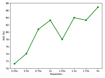
Figure 4: Frame-level AUCs obtained from anomaly detection on UCSD Ped2 with various frame resolutions. The base 1x is $160\times 120$.

As mentioned in Section 4.3, a possible reason of unexpected detections on UCSD Ped2 is the lack of useful details in cuboids due to the large distance between the camera and scene. To verify this hypothesis, we performed the assessment on this dataset with various frame resolutions scaled from the base one $160\times 120$. Since the patch size was still $10\times 10$, only the number of classes changed, e.g. 32 and 24 classes for $320\times 240$ frames. We trained all these models with only 40 epochs. This early stopping was performed since we focused on the potential of the proposed model architecture instead of attempting to find the best resolution for UCSD Ped2.

The AUCs obtained according to the normality score $\mathcal{S}_{R,x,y}$ are presented in Fig. 4, in which increasing the frame resolution tends to improve the model ability. Therefore, the experimental results of our model on UCSD Ped2 can be expected to be better when upscaling the input frames to appropriate dimensions.

4.5 Impact of adversarial training

In order to assess the impact of the adversarial training described in Section 3.3.3, we reimplemented the experiments using only the reconstruction and classification losses. Concretely, the discriminator $\mathcal{D}$ was not employed and the training was thus performed using the objective function $\mathcal{L}_{\mathcal{G}}$ in Eq. (3) where $\lambda_{\mathcal{G}}$ was assigned to 0. The corresponding experimental results are presented in Table 3. They show that using adversarial training improved the detection efficiency on most datasets except for the Traffic-Train. The reason is possibly the camera jitter which changed the structural texture of $10\times 10$ patches. Since such variations (and the sudden change of lighting) were unpredictable, the discriminator $\mathcal{D}$ might encounter difficulties in distinguishing real cuboids from the decoder’s output. Therefore, the use of adversarial training is unrecommended if the camera is unstable.

Dataset	Avenue†			UCSD Ped2†			Belleview‡			Traffic-Train‡
Normality score	$\mathcal{S}_{R}$	$\mathcal{S}_{x,y}$	$\mathcal{S}_{R,x,y}$	$\mathcal{S}_{R}$	$\mathcal{S}_{x,y}$	$\mathcal{S}_{R,x,y}$	$\mathcal{S}_{R}$	$\mathcal{S}_{x,y}$	$\mathcal{S}_{R,x,y}$	$\mathcal{S}_{R}$	$\mathcal{S}_{x,y}$	$\mathcal{S}_{R,x,y}$
w/ adv. training	80.1	80.6	82.8	76.3	76.8	84.3	68.6	82.7	73.1	40.0	64.4	50.5
w/o adv. training	80.1	80.3	82.5	74.3	74.0	77.4	68.3	81.7	72.5	42.9	67.4	54.9

Table 3: Comparison of anomaly detection ability between the proposed model and its modified version without adversarial training. ^†AUC. ^‡AP.

4.6 Impact of the decoder

Dataset	metric	w/	w/o
Avenue	AUC	80.6	80.3
Ped2	AUC	76.8	73.6
Belleview	AP	82.7	81.6
Train	AP	64.4	63.3

Table 4: Evaluation results on $\mathcal{S}_{x,y}$. Notations w/ and w/o are abbreviations of with and without the decoder, respectively.

Typically, an AE is applied to (unsupervisedly) learn the underlying features of data while a classification deep network can implicitly perform the feature extraction. Therefore, our hybrid network can theoretically work without the decoder. To evaluate its effect, we re-performed the experiments after removing the decoder in Fig. 1(a). Besides, the adversarial training (see Section 3.3.3) is also unnecessary since it focuses on enhancing the cuboids reconstructed from the AE. The network hence becomes a typical classification model with the objective function $\mathcal{L}_{C}$ in Eq. (2) and provides only two score maps $\mathcal{S}_{x}$ and $\mathcal{S}_{y}$ for each input frame. Table 4 presents a comparison of the efficiency of $\mathcal{S}_{x,y}$ for the two networks (with and without decoder). It shows that the learning of common cuboid features via the bottleneck AE has a certain contribution for anomaly detection. Some learned convolutional filters in the two networks are shown in the supplementary material.

5 Conclusion

In this paper, we propose a hybrid deep network combining both supervised and unsupervised learning perspectives for anomaly detection in surveillance videos. We designed a convolutional auto-encoder for learning common local appearance-motion features from small spatio-temporal cuboids. A classification sub-network is integrated to force such characteristics to be distinguishable for cuboids of different spatial locations. A novel anomaly score estimation/combination is presented and the impact of the decoder in our model is also discussed. The experiments on 4 benchmark datasets demonstrated the competitive performance of our hybrid network compared with state-of-the-art methodologies.

References

- Akcay et al. (2018) Samet Akcay, Amir Atapour-Abarghouei, and Toby P. Breckon. Ganomaly: Semisupervised anomaly detection via adversarial training. In Computer Vision – ACCV 2018, Cham, 2018. Springer International Publishing.
- Bensch et al. (2015) Robert Bensch, Thomas Brox, and Olaf Ronneberger. Spatiotemporal deformable prototypes for motion anomaly detection. In Xianghua Xie, Mark W. Jones, and Gary K. L. Tam, editors, Proceedings of the British Machine Vision Conference (BMVC), pages 189.1–189.12. BMVA Press, September 2015. ISBN 1-901725-53-7. 10.5244/C.29.189.
- Chatfield et al. (2014) Ken Chatfield, Karen Simonyan, Andrea Vedaldi, and Andrew Zisserman. Return of the devil in the details: Delving deep into convolutional nets. In Proceedings of the British Machine Vision Conference. BMVA Press, 2014. http://dx.doi.org/10.5244/C.28.6.
- Cheng et al. (2015) K. Cheng, Y. Chen, and W. Fang. Video anomaly detection and localization using hierarchical feature representation and gaussian process regression. In 2015 IEEE Conference on Computer Vision and Pattern Recognition (CVPR), pages 2909–2917, June 2015. 10.1109/CVPR.2015.7298909.
- Del Giorno et al. (2016) Allison Del Giorno, J. Andrew Bagnell, and Martial Hebert. A discriminative framework for anomaly detection in large videos. In Bastian Leibe, Jiri Matas, Nicu Sebe, and Max Welling, editors, Computer Vision – ECCV 2016, pages 334–349, Cham, 2016. Springer International Publishing. ISBN 978-3-319-46454-1.
- Dosovitskiy et al. (2015) A. Dosovitskiy, P. Fischer, E. Ilg, P. Häusser, C. Hazirbas, V. Golkov, P. v. d. Smagt, D. Cremers, and T. Brox. Flownet: Learning optical flow with convolutional networks. In 2015 IEEE International Conference on Computer Vision (ICCV), pages 2758–2766, Dec 2015. 10.1109/ICCV.2015.316.
- Goodfellow et al. (2014) Ian Goodfellow, Jean Pouget-Abadie, Mehdi Mirza, Bing Xu, David Warde-Farley, Sherjil Ozair, Aaron Courville, and Yoshua Bengio. Generative adversarial nets. In Z. Ghahramani, M. Welling, C. Cortes, N. D. Lawrence, and K. Q. Weinberger, editors, Advances in Neural Information Processing Systems 27, pages 2672–2680. Curran Associates, Inc., 2014.
- Hasan et al. (2016) M. Hasan, J. Choi, J. Neumann, A. K. Roy-Chowdhury, and L. S. Davis. Learning temporal regularity in video sequences. In 2016 IEEE Conference on Computer Vision and Pattern Recognition (CVPR), pages 733–742, June 2016. 10.1109/CVPR.2016.86.
- He et al. (2016) K. He, X. Zhang, S. Ren, and J. Sun. Deep residual learning for image recognition. In 2016 IEEE Conference on Computer Vision and Pattern Recognition (CVPR), pages 770–778, June 2016. 10.1109/CVPR.2016.90.
- He et al. (2017) K. He, G. Gkioxari, P. Dollár, and R. Girshick. Mask r-cnn. In 2017 IEEE International Conference on Computer Vision (ICCV), pages 2980–2988, Oct 2017. 10.1109/ICCV.2017.322.
- Hinami et al. (2017) R. Hinami, T. Mei, and S. Satoh. Joint detection and recounting of abnormal events by learning deep generic knowledge. In 2017 IEEE International Conference on Computer Vision (ICCV), pages 3639–3647, Oct 2017. 10.1109/ICCV.2017.391.
- Ilg et al. (2017) Eddy Ilg, Nikolaus Mayer, Tonmoy Saikia, Margret Keuper, Alexey Dosovitskiy, and Thomas Brox. Flownet 2.0: Evolution of optical flow estimation with deep networks. In The IEEE Conference on Computer Vision and Pattern Recognition (CVPR), July 2017.
- Ionescu et al. (2017) R. T. Ionescu, S. Smeureanu, B. Alexe, and M. Popescu. Unmasking the abnormal events in video. In 2017 IEEE International Conference on Computer Vision (ICCV), pages 2914–2922, Oct 2017. 10.1109/ICCV.2017.315.
- Isola et al. (2017) P. Isola, J. Zhu, T. Zhou, and A. A. Efros. Image-to-image translation with conditional adversarial networks. In 2017 IEEE Conference on Computer Vision and Pattern Recognition (CVPR), pages 5967–5976, July 2017. 10.1109/CVPR.2017.632.
- Kim and Grauman (2009) J. Kim and K. Grauman. Observe locally, infer globally: A space-time mrf for detecting abnormal activities with incremental updates. In 2009 IEEE Conference on Computer Vision and Pattern Recognition, pages 2921–2928, June 2009. 10.1109/CVPR.2009.5206569.
- Kingma and Ba (2015) Diederick P Kingma and Jimmy Ba. Adam: A method for stochastic optimization. In International Conference on Learning Representations (ICLR), 2015.
- Krizhevsky et al. (2012) Alex Krizhevsky, Ilya Sutskever, and Geoffrey E Hinton. Imagenet classification with deep convolutional neural networks. In F. Pereira, C. J. C. Burges, L. Bottou, and K. Q. Weinberger, editors, Advances in Neural Information Processing Systems 25, pages 1097–1105. Curran Associates, Inc., 2012.
- Li et al. (2014) W. Li, V. Mahadevan, and N. Vasconcelos. Anomaly detection and localization in crowded scenes. IEEE Transactions on Pattern Analysis and Machine Intelligence, 36(1):18–32, Jan 2014. ISSN 0162-8828. 10.1109/TPAMI.2013.111.
- Liu et al. (2018) Wen Liu, Weixin Luo, Dongze Lian, and Shenghua Gao. Future frame prediction for anomaly detection - a new baseline. In The IEEE Conference on Computer Vision and Pattern Recognition (CVPR), June 2018.
- Lu et al. (2013) C. Lu, J. Shi, and J. Jia. Abnormal event detection at 150 fps in matlab. In 2013 IEEE International Conference on Computer Vision, pages 2720–2727, Dec 2013. 10.1109/ICCV.2013.338.
- Luo et al. (2017) W. Luo, W. Liu, and S. Gao. A revisit of sparse coding based anomaly detection in stacked rnn framework. In 2017 IEEE International Conference on Computer Vision (ICCV), pages 341–349, Oct 2017. 10.1109/ICCV.2017.45.
- Maas et al. (2013) Andrew L. Maas, Awni Y. Hannun, and Andrew Y. Ng. Rectifier nonlinearities improve neural network acoustic models. In in ICML Workshop on Deep Learning for Audio, Speech and Language Processing, 2013.
- Mahadevan et al. (2010) V. Mahadevan, W. Li, V. Bhalodia, and N. Vasconcelos. Anomaly detection in crowded scenes. In 2010 IEEE Computer Society Conference on Computer Vision and Pattern Recognition, pages 1975–1981, June 2010. 10.1109/CVPR.2010.5539872.
- Mathieu et al. (2015) Michaël Mathieu, Camille Couprie, and Yann LeCun. Deep multi-scale video prediction beyond mean square error. CoRR, abs/1511.05440, 2015.
- Medioni et al. (2001) G. Medioni, I. Cohen, F. Bremond, S. Hongeng, and R. Nevatia. Event detection and analysis from video streams. IEEE Transactions on Pattern Analysis and Machine Intelligence, 23(8):873–889, Aug 2001. ISSN 0162-8828. 10.1109/34.946990.
- Nair and Hinton (2010) Vinod Nair and Geoffrey E. Hinton. Rectified linear units improve restricted boltzmann machines. In Proceedings of the 27th International Conference on International Conference on Machine Learning, ICML’10, pages 807–814, USA, 2010. Omnipress. ISBN 978-1-60558-907-7.
- Narasimhan and S. (2018) Medhini G. Narasimhan and Sowmya Kamath S. Dynamic video anomaly detection and localization using sparse denoising autoencoders. Multimedia Tools and Applications, 77(11):13173–13195, Jun 2018. ISSN 1573-7721. 10.1007/s11042-017-4940-2.
- Ravanbakhsh et al. (2017) M. Ravanbakhsh, M. Nabi, E. Sangineto, L. Marcenaro, C. Regazzoni, and N. Sebe. Abnormal event detection in videos using generative adversarial nets. In 2017 IEEE International Conference on Image Processing (ICIP), pages 1577–1581, Sep. 2017. 10.1109/ICIP.2017.8296547.
- Ravanbakhsh et al. (2019) M. Ravanbakhsh, E. Sangineto, M. Nabi, and N. Sebe. Training adversarial discriminators for cross-channel abnormal event detection in crowds. In 2019 IEEE Winter Conference on Applications of Computer Vision (WACV), pages 1896–1904, Jan 2019. 10.1109/WACV.2019.00206.
- Ren et al. (2015) Shaoqing Ren, Kaiming He, Ross Girshick, and Jian Sun. Faster r-cnn: Towards real-time object detection with region proposal networks. In C. Cortes, N. D. Lawrence, D. D. Lee, M. Sugiyama, and R. Garnett, editors, Advances in Neural Information Processing Systems 28, pages 91–99. Curran Associates, Inc., 2015.
- Sabokrou et al. (2018) Mohammad Sabokrou, Mohammad Khalooei, Mahmood Fathy, and Ehsan Adeli. Adversarially learned one-class classifier for novelty detection. In The IEEE Conference on Computer Vision and Pattern Recognition (CVPR), June 2018.
- Xu et al. (2015) Dan Xu, Elisa Ricci, Yan Yan, Jingkuan Song, and Nicu Sebe. Learning deep representations of appearance and motion for anomalous event detection. In Xianghua Xie, Mark W. Jones, and Gary K. L. Tam, editors, Proceedings of the British Machine Vision Conference (BMVC), pages 8.1–8.12. BMVA Press, September 2015. ISBN 1-901725-53-7. 10.5244/C.29.8.
- Xu et al. (2017) Dan Xu, Yan Yan, Elisa Ricci, and Nicu Sebe. Detecting anomalous events in videos by learning deep representations of appearance and motion. Computer Vision and Image Understanding, 156:117 – 127, 2017. ISSN 1077-3142. https://doi.org/10.1016/j.cviu.2016.10.010. Image and Video Understanding in Big Data.
- Zaharescu and Wildes (2010) Andrei Zaharescu and Richard Wildes. Anomalous behaviour detection using spatiotemporal oriented energies, subset inclusion histogram comparison and event-driven processing. In Kostas Daniilidis, Petros Maragos, and Nikos Paragios, editors, Computer Vision – ECCV 2010, pages 563–576, Berlin, Heidelberg, 2010. Springer Berlin Heidelberg. ISBN 978-3-642-15549-9.
- Zhang et al. (2009) T. Zhang, H. Lu, and S. Z. Li. Learning semantic scene models by object classification and trajectory clustering. In 2009 IEEE Conference on Computer Vision and Pattern Recognition, pages 1940–1947, June 2009. 10.1109/CVPR.2009.5206809.
- Zhang et al. (2016) Ying Zhang, Huchuan Lu, Lihe Zhang, Xiang Ruan, and Shun Sakai. Video anomaly detection based on locality sensitive hashing filters. Pattern Recognition, 59:302 – 311, 2016. ISSN 0031-3203. https://doi.org/10.1016/j.patcog.2015.11.018. Compositional Models and Structured Learning for Visual Recognition.
- Zhao et al. (2011) B. Zhao, L. Fei-Fei, and E. P. Xing. Online detection of unusual events in videos via dynamic sparse coding. In CVPR 2011, pages 3313–3320, June 2011. 10.1109/CVPR.2011.5995524.