Asymptotic enumeration of linear hypergraphs with given number of vertices and edges

Abstract

For $n\geq 3$, let $r=r(n)\geq 3$ be an integer. A hypergraph is $r$-uniform if each edge is a set of $r$ vertices, and is said to be linear if two edges intersect in at most one vertex. In this paper, the number of linear $r$-uniform hypergraphs on $n\to\infty$ vertices is determined asymptotically when the number of edges is $m(n)=o(r^{-3}n^{\frac{3}{2}})$. As one application, we find the probability of linearity for the independent-edge model of random $r$-uniform hypergraph when the expected number of edges is $o(r^{-3}n^{\frac{3}{2}})$. We also find the probability that a random $r$-uniform linear hypergraph with a given number of edges contains a given subhypergraph.

1 Introduction

For $n\geq 3$, let $r=r(n)$ and $\ell$ be integers such that $r=r(n)\geq 3$ and $2\leq\ell\leq r-1$. A hypergraph ${H}$ on vertex set $[n]$ is an $r$-uniform hypergraph ($r$-graph for short) if each edge is a set of $r$ vertices. An $r$-graph is called a partial Steiner $(n,r,\ell)$-system if every subset of size $\ell$ is contained in at most one edge of $H$. In particular, $(n,r,2)$-systems are also called linear hypergraphs, which implies that any two edges intersect in at most one vertex. Partial Steiner $(n,r,\ell)$-systems and the stronger version, Steiner $(n,r,\ell)$-systems, where every $\ell$-set is contained in precisely one edge of ${H}$, are widely studied combinatorial designs. Little is known about the number of distinct partial Steiner $(n,r,\ell)$-systems, denoted by $s(n,r,\ell)$. Grable and Phelps [7] used the Rödl nibble algorithm [11] to obtain an asymptotic formula for $\log s(n,r,\ell)$ as $\ell\leq r-1$ and $n\to\infty$. Asratian and Kuzjurin gave another proof [1].

An interesting problem is the enumeration of hypergraphs with given number of edges. Let $\mathcal{H}_{r}(n,m)$ denote the set of $r$-graphs on the vertex set $[n]$ with $m$ edges, and let $\mathcal{L}_{r}(n,m)$ denote the set of all linear hypergraphs in $\mathcal{H}_{r}(n,m)$.

Dudek et al. [6] used the switching method to obtain the asymptotic number of $k$-regular $r$-graphs for fixed $r$ and $n\to\infty$ with $k=o(n^{1/2})$. For $r=r(n)\geq 3$ an integer and a sequence of positive integers $\boldsymbol{k}=\boldsymbol{k}(n)=(k_{1},\ldots,k_{n})$, define $M=M(n)=\sum_{i=1}^{n}k_{i}$. Let $\mathcal{H}_{r}(\boldsymbol{k})$ denote the set of $r$-graphs on the vertex set $[n]$ with degree sequence $\boldsymbol{k}$, and $\mathcal{L}_{r}(\boldsymbol{k})$ denote the set of all linear hypergraphs in $\mathcal{H}_{r}(\boldsymbol{k})$. Blinovsky and Greenhill [3, 4] extended the asymptotic enumeration result on the number of $k$-regular $r$-graphs to the general $\mathcal{H}_{r}(\boldsymbol{k})$ when $r^{4}k_{\rm max}^{3}=o(M)$ and $n\to\infty$. By relating the incidence matrix of a hypergraph to the biadjacency matrix of a bipartite graph, they used switching arguments together with previous enumeration results for bipartite graphs to obtain the asymptotic enumeration formula for $\mathcal{L}_{r}(\boldsymbol{k})$ provided $r^{4}k_{\rm max}^{4}(k_{\rm max}+r)=o(M)$ and $n\to\infty$ [4]. Recently, Balogh and Li [2] obtained an upper bound on the total number of linear $r$-graphs with given girth for fixed $r\geq 3$.

Apart from these few results, the literature on the enumeration of linear hypergraphs is very sparse. In particular, there seems to be no asymptotic enumeration of linear hypergraphs by the number of edges, which is the subject of this paper. The result of Blinovsky and Greenhill [4] could in principle be summed over degree sequences to obtain $\mathcal{L}_{r}(n,m)$ for $m=o\bigl{(}\min\{r^{-2}n^{\frac{5}{4}},r^{-\frac{8}{3}}n^{\frac{4}{3}}\}\bigr{)}$, but we prefer a direct switching approach. Note that $m=O(r^{-2}n^{2})$ for all linear hypergraphs; we get as far as $m=o(r^{-3}n^{\frac{3}{2}})$.

Our application of the switching method combines several different switching operations into a single computation, which was previously used in [8] to count sparse $0$-$1$ matrices with irregular row and column sums, in [9] to count sparse nonnegative integer matrices with specified row and column sums, and in [10] to count sparse multigraphs with given degrees.

We will use the falling factorial $[x]_{t}=x(x-1)\cdots(x-t+1)$ and adopt $N$ as an abbreviation for $\binom{n}{r}$. All asymptotics are with respect to $n\to\infty$. Our main theorem is the following.

Theorem 1.1.

Let $r=r(n)\geq 3$ and $m=m(n)$ be integers with $m=o(r^{-3}n^{\frac{3}{2}})$. Then, as $n\to\infty$,

$$|\mathcal{L}_{r}(n,m)| =\binom{N}{m}\exp\biggl{[}-\frac{[r]_{2}^{2}[m]_{2}}{4n^{2}}-\frac{[r]_{2}^{3}(3r^{2}-15r+20)m^{3}}{24n^{4}}+O\Bigl{(}\frac{r^{6}m^{2}}{n^{3}}\Bigr{)}\biggr{]}$$ (1.1)

$$={\frac{N^{m}}{m!}}\exp\biggl{[}-\frac{[r]_{2}^{2}[m]_{2}}{4n^{2}}-\frac{[r]_{2}^{3}(3r^{2}-15r+20)m^{3}}{24n^{4}}+O\Bigl{(}\frac{r^{6}m^{2}}{n^{3}}\Bigr{)}\biggr{]}.$$

Proof of Theorem 1.1.

Note that the condition $m=o(r^{-3}n^{\frac{3}{2}})$ implies that either $m=0$ or $r=o(n^{\frac{1}{2}})$. In the former case the theorem is trivially true, while in the latter we can apply Remark 4.5 and Lemma 6.6 to obtain (1.1) for $r^{-2}n\leq m=o(r^{-3}n^{\frac{3}{2}})$. Equivalent expressions follow from Remark 7.3 and Lemma 7.6 when $\log(r^{-2}n)\leq m=O(r^{-2}m)$ and from Remark 8.2 and Lemma 8.5 when $1\leq m=O(\log(r^{-2}n))$. ∎

Let $\mathbb{P}_{r}(n,m)$ denote the probability that an $r$-graph $H\in\mathcal{H}_{r}(n,m)$ chosen uniformly at random is linear. Then

$$|\mathcal{L}_{r}(n,m)|=\binom{N}{m}\mathbb{P}_{r}(n,m).$$

Hence, our task is reduced to computing $\mathbb{P}_{r}(n,m)$ and it suffices to show that $\mathbb{P}_{r}(n,m)$ equals the exponential factor in Theorem 1.1.

Recall that a random $r$-graph ${H}_{r}(n,p)=([n],E_{n,p})$ refers to an $r$-graph on the vertex set $[n]$, where each $r$-set is an edge randomly and independently with probability $p$. Also it might be surmised that random hypergraphs with edge probability $p$ have about the same probability of being linear as a random hypergraph with $Np$ edges, that is not the case when $Np$ is moderately large. Let $\mathcal{L}_{r}(n)$ be the set of all linear $r$-graphs with $n$ vertices.

Theorem 1.2.

Let $r=r(n)\geq 3$ and let $pN=m_{0}$ with $m_{0}=o(r^{-3}n^{\frac{3}{2}})$. Then, as $n\to\infty$,

$$\mathbb{P} [H_{r}(n,p)\in\mathcal{L}_{r}(n)]$$

$$=\begin{cases}\exp\Bigl{[}-\frac{[r]_{2}^{2}m_{0}^{2}}{4n^{2}}+O\bigl{(}\frac{r^{6}m_{0}^{2}}{n^{3}}\bigr{)}\Bigr{]},&\text{ if }m_{0}=O(r^{-2}n);\\[8.61108pt] \exp\Bigl{[}-\frac{[r]_{2}^{2}m_{0}^{2}}{4n^{2}}+\frac{[r]_{2}^{3}(3r-5)m_{0}^{3}}{6n^{4}}+O\bigl{(}\frac{\log^{3}(r^{-2}n)}{\sqrt{m_{0}}}+\frac{r^{6}m_{0}^{2}}{n^{3}}\bigr{)}\Bigr{]},&\text{ if }r^{-2}n\leq m_{0}=o(r^{-3}n^{\frac{3}{2}}).\end{cases}$$

From the calculations in the proof of Theorem 1.2, we have a corollary about the distribution on the number of edges of $H_{r}(n,p)$ conditioned on it being linear.

Corollary 1.3.

Let $r=r(n)\geq 3$ and let $Np=m_{0}$ with $r^{-2}n\leq m_{0}=o(r^{-3}n^{\frac{3}{2}})$. Suppose that $n\to\infty$. Then the number of edges of $H_{r}(n,p)$ conditioned on being linear converges in distribution to the normal distribution with mean $m_{0}-\frac{[r]_{2}^{2}m_{0}^{2}}{2n^{2}}$ and variance $m_{0}$.

Consider $H\in\mathcal{L}_{r}(n,m)$ chosen uniformly at random. Using a similar switching method, we also obtain the probability that $H$ contains a given hypergraph as a subhypergraph.

Theorem 1.4.

Let $r=r(n)\geq 3$, $m=m(n)$ and $k=k(n)$ be integers with $m=o(r^{-3}n^{\frac{3}{2}})$ and $k=o\bigl{(}\frac{n^{3}}{r^{6}m^{2}}\bigr{)}$. Let $K=K(n)$ be a linear $r$-graph on $n$ vertices with $k$ edges. Let $H\in\mathcal{L}_{r}(n,m)$ be chosen uniformly at random. Then, as $n\to\infty$,

$$\mathbb{P}[K\subseteq H]=\frac{[m]_{k}}{N^{k}}\exp\biggl{[}\frac{[r]_{2}^{2}k^{2}}{4n^{2}}+O\Bigl{(}\frac{r^{4}k}{n^{2}}+\min\Bigl{\{}\frac{r^{6}m^{2}k}{n^{3}},\frac{r^{5}mk}{n^{2}}\Bigr{\}}\Bigr{)}\biggr{]}.$$

The remainder of the paper is structured as follows. Notation and auxiliary results are presented in Section 2. From Section 3 to Section 6, we mainly consider the case $r^{-2}n\leq m=o(r^{-3}n^{\frac{3}{2}})$. In Section 3, we define subsets $\mathcal{H}^{+}_{r}(n,m)$ and $\mathcal{H}^{++}_{r}(n,m)$ of $\mathcal{H}_{r}(n,m)$ and show that they are almost all of $\mathcal{H}_{r}(n,m)$. In Section 4, we show that the same is true when $\mathcal{H}^{+}_{r}(n,m)$ and $\mathcal{H}^{++}_{r}(n,m)$ are restricted by certain counts of clusters of edges that overlap in more than one vertex. We define four other kinds of switchings on $r$-graphs in $\mathcal{H}_{r}^{+}(n,m)$ which are used to remove some hyperedges with two or more common vertices, and analyze these switchings in Section 5. In Section 6, we complete the enumeration for the case $r^{-2}n\leq m=o(r^{-3}n^{\frac{3}{2}})$ with the help of some calculations performed in [8, 9, 10]. In Sections 7–8, we consider the cases $\log(r^{-2}n)\leq m=O(r^{-2}n)$ and $1\leq m=O(\log(r^{-2}n))$, respectively. In Section 9, we prove Theorem 1.2, while in Section 10, we prove Theorem 1.4.

2 Notation and auxiliary results

To state our results precisely, we need some definitions. Let $H$ be an $r$-graph in $\mathcal{H}_{r}(n,m)$. For $U\subseteq[n]$, the codegree of $U$ in $H$, denoted by $\operatorname{codeg}({U})$, is the number of edges of $H$ containing $U$. In particular, if $U=\{v\}$ for $v\in[n]$ then $\operatorname{codeg}({U})$ is the degree of $v$ in $H$, denoted by $\deg(v)$. Any $2$-set $\{x,y\}\subseteq[n]$ in an edge $e$ of $H$ is called a link of $e$ if $\operatorname{codeg}({x,y})\geq 2$. Two edges $e_{i}$ and $e_{j}$ in $H$ are called linked edges if $|e_{i}\cap e_{j}|=2$.

Let $G_{H}$ be a simple graph whose vertices are the edges of $H$, with two vertices of $G$ adjacent iff the corresponding edges of $H$ are linked. An edge induced subgraph of $H$ corresponding to a non-trivial component of $G_{H}$ is called a cluster of $H$. The standard asymptotic notations $o$ and $O$ refer to $n\to\infty$. The floor and ceiling signs are omitted whenever they are not crucial.

In order to identify several events which have low probabilities in the uniform probability space $\mathcal{H}_{r}(n,m)$ as $m=o(r^{-3}n^{\frac{3}{2}})$, the following lemmas will be useful.

Lemma 2.1.

Let $r=r(n)\geq 3$, $t=t(n)\geq 1$ be integers. Let $e_{1},\ldots,e_{t}$ be distinct $r$-sets of $[n]$ and $H$ be an $r$-graph that is chosen uniformly at random from $\mathcal{H}_{r}(n,m)$. Then the probability that $e_{1},\ldots,e_{t}$ are edges of $H$ is at most $\bigl{(}\frac{m}{N}\bigr{)}^{t}$.

Proof.

Since $H$ is an $r$-graph that is chosen uniformly at random from $\mathcal{H}_{r}(n,m)$, the probability that $e_{1},\ldots,e_{t}$ are edges of $H$ is

$$\frac{\binom{N-t}{m-t}}{\binom{N}{m}} =\frac{[m]_{t}}{[N]_{t}}=\prod_{i=0}^{t-1}\frac{m-i}{N-i}\leq\Bigl{(}\frac{m}{N}\Bigr{)}^{t}.\qed$$

Lemma 2.2.

Let $r=r(n)\geq 3$ be an integer with $r=o(n^{\frac{1}{2}})$. Let $t$ and $\alpha$ be integers such that $t=O(1)$ and $0\leq\alpha\leq rt$. If a hypergraph $H$ is chosen uniformly at random from $\mathcal{H}_{r}(n,m)$, then the expected number of sets of $t$ edges of $H$ whose union has $rt-\alpha$ or fewer vertices is $O\bigl{(}t^{\alpha}r^{2\alpha}m^{t}n^{-\alpha})$.

Proof.

Let $e_{1},\ldots,e_{t}$ be distinct $r$-sets of $[n]$. According to Lemma 2.1, the probability that $e_{1},\ldots,e_{t}$ are edges of $H$ is at most $(m/N)^{t}$. Here, we firstly count how many $e_{1},\ldots,e_{t}$ such that $|e_{1}\cup\cdots\cup e_{t}|=rt-\beta$ for some $\beta\geq\alpha$.

Suppose that there is a sequence among the edges $\{e_{1},\ldots,e_{t}\}$ and we have chosen the edges $\{e_{1},\ldots,e_{i-1}\}$, where $2\leq i\leq t$. Let $a_{i}=|(e_{1}\cup\cdots\cup e_{i-1})\cap e_{i}|$, thus we have $\sum_{i=2}^{t}a_{i}=\beta$ and

$$O\biggl{(}N\prod_{i=2}^{t}(tr)^{a_{i}}\binom{n}{r-a_{i}}\biggr{)}$$

ways to choose $\{e_{1},\ldots,e_{t}\}$. The expected number of these $t$ edges is

$$O\biggl{(}\Bigl{(}\frac{m}{N}\Bigr{)}^{t}N\prod_{i=2}^{t}(tr)^{a_{i}}\binom{n}{r-a_{i}}\biggr{)} =O\biggl{(}m^{t}t^{\beta}r^{\beta}\prod_{i=2}^{t}\frac{[r]_{a_{i}}}{[n-r]_{a_{i}}}\biggr{)}$$

$$=O\biggl{(}m^{t}t^{\beta}r^{\beta}\prod_{i=2}^{t}\Bigl{(}\frac{r}{n-r}\Bigr{)}^{a_{i}}\biggr{)}=O\biggl{(}\frac{t^{\beta}m^{t}r^{2\beta}}{n^{\beta}}\biggr{)},$$

where we use the fact that $\prod_{j=0}^{a_{i}-1}\frac{r-j}{n-r-j}\leq\bigl{(}\frac{r}{n-r}\bigr{)}^{a_{i}}$ is true as $r\leq\frac{n}{2}$ and $\bigl{(}\frac{r}{n-r}\bigr{)}^{a_{i}}=O((\frac{r}{n})^{a_{i}})$ because $a_{i}<r$, $r=o(n^{\frac{1}{2}})$ and $a_{i}r=o(n)$.

The expected number of sets of $t$ edges whose union has at most $rt-\alpha$ vertices is

$$O\biggl{(}\sum_{\beta\geq\alpha}\frac{t^{\beta}m^{t}r^{2\beta}}{n^{\beta}}\biggr{)}=O\biggl{(}\frac{t^{\alpha}m^{t}r^{2\alpha}}{n^{\alpha}}\biggr{)},$$

because $\beta=\alpha$ corresponds to the largest term as $t=O(1)$ and $r=o(n^{\frac{1}{2}})$.∎

Remark 2.3.

Throughout the following sections we assume that $n\to\infty$. From Sections 3–6, we assume that $r^{-2}n\leq m=o(r^{-3}n^{\frac{3}{2}})$. In Sections 7–8 , we assume that $\log(r^{-2}n)\leq m=O(r^{-2}n)$ and $1\leq m=O(\log(r^{-2}n))$, respectively. Recall that these conditions all imply that $r=o(n^{\frac{1}{2}})$.

3 Two important subsets of $\mathcal{H}_{r}(n,m)$

Define

$$\begin{split}M_{0}^{*}&=\biggl{\lceil}\log(r^{-2}n)+\frac{3^{4}r^{2}m}{n}\biggr{\rceil},\\ M_{0}&=\biggl{\lceil}\log(r^{-2}n)+\frac{3^{4}r^{2}m}{n}\biggr{\rceil}+3,\\ M_{1}&=\biggl{\lceil}\log(r^{-2}n)+\frac{3^{4}r^{8}m^{3}}{2n^{4}}\biggr{\rceil},\\ M_{2}&=\biggl{\lceil}\log(r^{-2}n)+\frac{3^{4}r^{7}m^{3}}{2n^{4}}\biggr{\rceil},\\ M_{3}&=\biggl{\lceil}\log(r^{-2}n)+\frac{3^{4}r^{6}m^{3}}{2n^{4}}\biggr{\rceil},\\ M_{4}&=\biggl{\lceil}\log(r^{-2}n)+\frac{3^{4}r^{4}m^{2}}{2n^{2}}\biggr{\rceil}.\end{split}$$ (3.1)

Now define $\mathcal{H}_{r}^{+}(n,m)\subseteq\mathcal{H}_{r}(n,m)$ to be the set of $r$-graphs $H$ which satisfy the following properties $\bf(a)$ to $\bf(g)$.

$\bf(a)$  The intersection of any two edges contains at most two vertices.

$\bf(b)$  $H$ only contains the four types of clusters that are shown in Figure 1. (This implies that any three edges of $H$ involve at least $3r-4$ vertices and any four edges involve at least $4r-5$ vertices. Thus, if there are three edges of $H$, for example $\{e_{1},e_{2},e_{3}\}$, such that $|e_{1}\cup e_{2}\cup e_{3}|=3r-4$, then $|e\cap(e_{1}\cup e_{2}\cup e_{3})|\leq 1$ for any edge $e$ other than $\{e_{1},e_{2},e_{3}\}$ of $H$.)

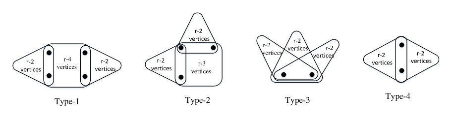
Figure 1: The four types of clusters allowed in $H\in\mathcal{H}_{r}^{+}(n,m)$.

$\bf(c)$ The intersection of any two clusters contains at most one vertex.

$\bf(d)$ Any three distinct Type-$1$, Type-$2$ or Type-$3$ clusters involve at least $9r-13$ vertices. (Together with $\bf(c)$, this implies that if a pair of Type-$1$, Type-$2$ or Type-$3$ clusters have exactly one common vertex, then any other Type-$1$, Type-$2$ or Type-$3$ clusters of $H$ must be vertex-disjoint from them.)

$\bf(e)$ Any three distinct Type-$4$ clusters involve at least $6r-8$ vertices. (Together with $\bf(c)$, this implies that if a pair of Type-$4$ clusters of $H$ have exactly one common vertex, then any other Type-$4$ cluster of $H$ shares at most one vertex with them.)

$\bf(f)$ There are at most $M_{i}$ Type-$i$ clusters, for $1\leq i\leq 4$.

$\bf(g)$ $\deg(v)\leq M_{0}$ for every vertex $v\in[n]$.

We further define $\mathcal{H}_{r}^{++}(n,m)\subseteq\mathcal{H}_{r}^{+}(n,m)$ to be the set of $r$-graphs $H$ by replacing the property $\bf(g)$ with a stronger constraint $\bf(g^{*})$.

$\bf(g^{*})$ $\deg(v)\leq M_{0}^{*}$ for every vertex $v\in[n]$.

Remark 3.1.

From property $\bf(g)$, it is natural to obtain

$$\sum_{v\in[n]}\binom{\deg(v)}{2}=O\Bigl{(}M_{0}\sum_{v\in[n]}\deg(v)\Bigr{)}=O\bigl{(}rmM_{0}\bigr{)}=O\Bigl{(}rm\log(r^{-2}n)+\frac{r^{3}m^{2}}{n}\Bigr{)}$$

for $H\in\mathcal{H}_{r}^{+}(n,m)$.

We now show that the expected number of $r$-graphs in $\mathcal{H}_{r}(n,m)$ not satisfying the properties of $\mathcal{H}^{+}_{r}(n,m)$ and $\mathcal{H}^{++}_{r}(n,m)$ is quite small, which implies that these $r$-graphs make asymptotically insignificant contributions. The removal of these $r$-graphs from our main proof will lead to some welcome simplifications.

Theorem 3.2.

Suppose that $r^{-2}n\leq m=o(r^{-3}n^{\frac{3}{2}})$ and $n\to\infty$. Then

$$\frac{|\mathcal{H}^{+}_{r}(n,m)|}{|\mathcal{H}_{r}(n,m)|}=1-O\Bigl{(}\frac{r^{6}m^{2}}{n^{3}}\Bigr{)},\quad\frac{|\mathcal{H}^{++}_{r}(n,m)|}{|\mathcal{H}_{r}(n,m)|}=1-O\Bigl{(}\frac{r^{6}m^{2}}{n^{3}}\Bigr{)}.$$

Proof.

Consider $H\in\mathcal{H}_{r}(n,m)$ chosen uniformly at random. It’s enough for us to prove the second equation. We apply Lemma 2.2 several times to show that $H$ satisfies the properties $\bf(a)$-$\bf(g^{*})$ with probability $1-O\bigl{(}\frac{r^{6}m^{2}}{n^{3}}\bigr{)}$.

$\bf(a)$  Applying Lemma 2.2 with $t=2$ and $\alpha=3$, the expected number of two edges involving at most $2r-3$ vertices is $O\bigl{(}\frac{r^{6}m^{2}}{n^{3}}\bigr{)}$. Hence, the property $\bf(a)$ holds with probability $1-O\bigl{(}\frac{r^{6}m^{2}}{n^{3}}\bigr{)}$.

$\bf(b)$ Applying Lemma 2.2 with $t=3$ and $\alpha=5$, the expected number of three edges involving at most $3r-5$ vertices is

$$O\Bigl{(}\frac{r^{10}m^{3}}{n^{5}}\Bigr{)}=O\Bigl{(}\frac{r^{6}m^{2}}{n^{3}}\Bigr{)},$$

where the last equality is true because $m=o(r^{-3}n^{\frac{3}{2}})$.

Similarly, applying Lemma 2.2 with $t=4$ and $\alpha=6$, the expected number of four edges involving at most $4r-6$ vertices is

$$O\Bigl{(}\frac{r^{12}m^{4}}{n^{6}}\Bigr{)}=O\Bigl{(}\frac{r^{6}m^{2}}{n^{3}}\Bigr{)}.$$

If there is a cluster with four or more edges, then there must be four edges involving at most $4r-6$ vertices. Hence, every cluster contains at most three edges and the property $\bf(b)$ holds with probability $1-O\bigl{(}\frac{r^{6}m^{2}}{n^{3}}\bigr{)}$.

$\bf(c)$ Applying Lemma 2.2, the expected number of two clusters such that their intersection contains two or more vertices is

$$O\Bigl{(}\frac{r^{20}m^{6}}{n^{10}}+\frac{r^{16}m^{5}}{n^{8}}+\frac{r^{12}m^{4}}{n^{6}}\Bigr{)}=O\Bigl{(}\frac{r^{6}m^{2}}{n^{3}}\Bigr{)},$$

where the first term arises from the case between Type-$1$ (or Type-$2$ or Type-$3$) cluster and Type-$1$ (or Type-$2$ or Type-$3$) cluster and there are at most $6r-10$ vertices if their intersection contains at least two vertices, the second term arises from the case between Type-$1$ (or Type-$2$ or Type-$3$) cluster and Type-$4$ cluster and there are at most $5r-8$ vertices if their intersection contains at least two vertices, while the last term arises from the case between Type-$4$ cluster and Type-$4$ cluster and there are at most $4r-6$ vertices if their intersection contains at least two vertices. Hence, the property $\bf(c)$ holds with probability $1-O\bigl{(}\frac{r^{6}m^{2}}{n^{3}}\bigr{)}$.

$\bf(d)$ The expected number of three Type-$1$, Type-$2$ or Type-$3$ clusters involving at most $9r-14$ vertices is

$$O\Bigl{(}\frac{r^{28}m^{9}}{n^{14}}\Bigr{)}=O\Bigl{(}\frac{r^{6}m^{2}}{n^{3}}\Bigr{)}.$$

Hence, the property $\bf(d)$ holds with probability $1-O\bigl{(}\frac{r^{6}m^{2}}{n^{3}}\bigr{)}$.

$\bf(e)$  The expected number of three Type-$4$ clusters involving at most $6r-9$ vertices is

$$O\Bigl{(}\frac{r^{18}m^{6}}{n^{9}}\Bigr{)}=O\Bigl{(}\frac{r^{6}m^{2}}{n^{3}}\Bigr{)}.$$

Hence, the property $\bf(e)$ holds with probability $1-O\bigl{(}\frac{r^{6}m^{2}}{n^{3}}\bigr{)}$.

$\bf(f)$ Define four events $\mathcal{E}_{i}$ as

$$\mathcal{E}_{i}=\bigl{\{}\text{There are at most $M_{i}$ Type-$i$ clusters in $H$}\bigr{\}},$$

and $\mathcal{\overline{E}}_{i}$ as the complement of the event $\mathcal{E}_{i}$, where $1\leq i\leq 4$. We show that $\mathbb{P}[\mathcal{E}_{i}]=1-O\bigl{(}\frac{r^{6}m^{2}}{n^{3}}\bigr{)}$ for $1\leq i\leq 4$.

Let

$$Q_{1}=\biggl{\lceil}\log(r^{-2}n)+\frac{3^{4}r^{8}m^{3}}{4n^{4}}\biggr{\rceil}$$

and define $\ell_{1}=Q_{1}+1$. We first show that the expected number of sets of $\ell_{1}$ vertex-disjoint Type-$1$ clusters in $H$ is $O\bigl{(}\frac{r^{6}}{n^{3}}\bigr{)}$. These $\ell_{1}$ vertex-disjoint Type-$1$ clusters contain $3\ell_{1}$ edges and $(3r-4)\ell_{1}$ vertices. Note that Lemma 2.2 is not appropriate here because $3\ell_{1}$ is not a constant.

By Lemma 2.1, it follows that the expected number of sets of $\ell_{1}$ vertex-disjoint Type-$1$ clusters in $H$ is at most

$$\binom{n}{(3r-4)\ell_{1}} \binom{(3r-4)\ell_{1}}{3r-4,\ldots,3r-4}\frac{1}{\ell_{1}!}\biggl{[}\binom{3r-4}{r}\binom{r}{4}\binom{4}{2}\binom{2r-4}{r-2}\biggr{]}^{\ell_{1}}\biggl{(}\frac{m}{N}\biggr{)}^{3\ell_{1}}$$

$$=O\biggl{(}\biggl{(}\frac{[r]_{4}[r]_{2}^{2}em^{3}}{4\ell_{1}n^{4}}\biggr{)}^{\ell_{1}}\biggr{)}=O\Bigl{(}\Bigl{(}\frac{e}{3^{4}}\Bigr{)}^{\ell_{1}}\Bigr{)}=O\Bigl{(}\frac{r^{6}}{n^{3}}\Bigr{)},$$

where the first two equalities are true because $\ell_{1}!\geq\bigl{(}\frac{\ell_{1}}{e}\bigr{)}^{\ell_{1}}$ and $\ell_{1}>\frac{3^{4}r^{8}m^{3}}{4n^{4}}$, and the last equality is true because of the assumption $\ell_{1}>\log(r^{-2}n)$.

Assuming that property $\bf(d)$ holds, any Type-$1$ cluster is either vertex-disjoint from all other Type-$1$ clusters of $H$, or shares one vertex with precisely one other Type-$1$ cluster of $H$, then it follows that $\mathbb{P}[\mathcal{\overline{E}}_{1}\mid\text{Property {\bf(d)} holds}]=O\bigl{(}\frac{r^{6}}{n^{3}}\bigr{)}$. By the total probability formula, we have

$$\mathbb{P}[\mathcal{\overline{E}}_{1}]\leq\mathbb{P}[\text{Property {\bf(d)} does not hold}]+\mathbb{P}[\mathcal{\overline{E}}_{1}\mid\text{Property {\bf(d)} holds}]=O\Bigl{(}\frac{r^{6}m^{2}}{n^{3}}\Bigr{)}$$

and $\mathbb{P}\left[\mathcal{E}_{1}\right]=1-O\bigl{(}\frac{r^{6}m^{2}}{n^{3}}\bigr{)}$. Similarly, we have $\mathbb{P}\left[\mathcal{E}_{2}\right]=1-O\bigl{(}\frac{r^{6}m^{2}}{n^{3}}\bigr{)}$, $\mathbb{P}\left[\mathcal{E}_{3}\right]=1-O\bigl{(}\frac{r^{6}m^{2}}{n^{3}}\bigr{)}$.

At last, we show that $\mathbb{P}[\mathcal{E}_{4}]=1-O\bigl{(}\frac{r^{6}m^{2}}{n^{3}}\bigr{)}$ is also true. Let $\ell_{4}=M_{4}+1$. Let $\{x_{i},y_{i}\}\in\binom{[n]}{2}$ be a set of $\ell_{4}$ links with edges $e_{i}$ and $e_{i}^{\prime}$, here $i\in\{1,\ldots,\ell_{4}\}$. These $\ell_{4}$ links are called paired-distinct if these $2\ell_{4}$ edges are all distinct. Assuming the property $\bf(b)$ holds, note that the number of Type-$4$ clusters is no greater than the number of paired-distinct links. Define a event $\mathcal{E}_{4}^{\prime}$ as

$$\mathcal{E}_{4}^{\prime}=\bigl{\{}\text{There are at most $M_{4}$ paired-distinct links in $H$}\bigr{\}},$$

and $\mathcal{\overline{E}}_{4}^{\prime}$ as the complement of the event $\mathcal{E}_{4}^{\prime}$. We firstly show that $\mathbb{P}[\mathcal{\overline{E}}_{4}^{\prime}]=O\bigl{(}\frac{r^{6}}{n^{3}}\bigr{)}$ by

$$\mathbb{P}\bigl{[}\mathcal{\overline{E}}_{4}^{\prime}\bigr{]}=O\biggl{(}\binom{n}{r-2}^{2\ell_{4}}\binom{\binom{n}{2}}{\ell_{4}}\biggl{(}\frac{m}{N}\biggr{)}^{2\ell_{4}}\biggr{)}=O\biggl{(}\Bigl{(}\frac{r^{4}em^{2}}{2\ell_{4}n^{2}}\Bigr{)}^{\ell_{4}}\biggr{)}=O\Bigl{(}\frac{r^{6}}{n^{3}}\Bigr{)},$$

where the last two equalities are true because $\ell_{4}>\frac{3^{4}r^{4}m^{2}}{2n^{2}}$ and $\ell_{4}>\log(r^{-2}n)$. Then it follows that $\mathbb{P}[\mathcal{\overline{E}}_{4}\mid\text{Property {\bf(b)} holds}]\leq\mathbb{P}[\mathcal{\overline{E}}_{4}^{\prime}]=O\bigl{(}\frac{r^{6}}{n^{3}}\bigr{)}$. By the law of total probability,

$$\mathbb{P}[\mathcal{\overline{E}}_{4}]\leq\mathbb{P}[\text{Property {\bf(b)} does not hold}]+\mathbb{P}[\mathcal{\overline{E}}_{4}\mid\text{Property {\bf(b)} holds}]=O\Bigl{(}\frac{r^{6}m^{2}}{n^{3}}\Bigr{)}.$$

$\bf(g^{*})$  Define $d=M_{0}^{*}+1$. The expected number of vertices $v$ such that $\deg(v)\geq d$ is

$$n\binom{n-1}{r-1}^{d}\frac{1}{d!}\Bigl{(}\frac{m}{N}\Bigr{)}^{d}=O\Bigl{(}n\Bigl{(}\frac{emr}{dn}\Bigr{)}^{d}\Bigr{)}=O\Bigl{(}n\Bigl{(}\frac{e}{3^{4}r}\Bigr{)}^{d}\Bigr{)}=O\Bigl{(}\frac{r^{6}}{n^{3}}\Bigr{)},$$

where the second equality is true because $d!\geq\bigl{(}\frac{d}{e}\bigr{)}^{d}$, and the last equality is true because of the assumption $d>M_{0}^{*}$ made in (3.1). Thus, there are no vertices with degree at least $d$ in $H$ holds with probability $1-O\bigl{(}\frac{r^{6}}{n^{3}}\bigr{)}$.

This completes the proof of Theorem 3.2. ∎

Remark 3.3.

For nonnegative integers $h_{1}$, $h_{2}$, $h_{3}$ and $h_{4}$, define $\mathcal{C}_{h_{1},h_{2},h_{3},h_{4}}^{+}$ to be the set of $r$-graphs in $H\in\mathcal{H}_{r}^{+}(n,m)$ with exactly $h_{i}$ clusters of Type $i$, for $1\leq i\leq 4$. Define $\mathcal{C}_{h_{1},h_{2},h_{3},h_{4}}^{++}$ similarly. By the definitions of $H\in\mathcal{H}_{r}^{+}(n,m)$ and $H\in\mathcal{H}_{r}^{++}(n,m)$ we have

$$|\mathcal{H}_{r}^{+}(n,m)| =\sum_{h_{4}=0}^{M_{4}}\sum_{h_{3}=0}^{M_{3}}\sum_{h_{2}=0}^{M_{2}}\sum_{h_{1}=0}^{M_{1}}|\mathcal{C}_{h_{1},h_{2},h_{3},h_{4}}^{+}|,$$

$$|\mathcal{H}_{r}^{++}(n,m)| =\sum_{h_{4}=0}^{M_{4}}\sum_{h_{3}=0}^{M_{3}}\sum_{h_{2}=0}^{M_{2}}\sum_{h_{1}=0}^{M_{1}}|\mathcal{C}_{h_{1},h_{2},h_{3},h_{4}}^{++}|.$$

We will estimate the relative sizes of these subsets by means of switching operations. The following is an essential tool that we will use repeatedly.

Lemma 3.4.

Assume that $r^{-2}n\leq m=o(r^{-3}n^{\frac{3}{2}})$. Let $H\in\mathcal{H}_{r}^{+}(n,m-\xi)$ and $N_{t}$ be the set of $t$-sets of $[n]$ of which no two vertices belong to the same edge of $H$, where $r\leq t\leq 3r-4$ and $\xi=O(1)$. Suppose that $n\to\infty$. Then

$$|N_{t}|=\biggl{[}\binom{n}{t}-\binom{r}{2}m\binom{n-2}{t-2}\biggr{]}\biggl{(}1+O\Bigl{(}\frac{r^{6}mn\log(r^{-2}n)+r^{8}m^{2}}{n^{4}}\Bigr{)}\biggr{)}.$$

Proof.

We will use inclusion-exclusion. Let $A_{e(i,j)}$ be the event that a $t$-set of $[n]$ contains two vertices $i$ and $j$ of the edge $e$. Thus, we have

$$\binom{n}{t}-\sum_{\{e,\{i,j\}\}}|A_{e(i,j)}|\leq|N_{t}|\leq\binom{n}{t}-\sum_{\{e,\{i,j\}\}}|A_{e(i,j)}|+\sum_{\{e,\{i,j\}\}\neq\{e^{\prime},\{i^{\prime},j^{\prime}\}\}}|A_{e(i,j)}\cap A_{e^{\prime}(i^{\prime},j^{\prime})}|.$$

Clearly, $|A_{e(i,j)}|=\binom{n-2}{t-2}$ for each edge $e$ and $\{i,j\}\subset e$. We have $|N_{t}|\geq\binom{n}{t}-\binom{r}{2}(m-\xi)\binom{n-2}{t-2}$.

Now we consider the upper bound. For the case $e=e^{\prime}$, we have

$$\sum_{\{e,\{i,j\}\}\neq\{e^{\prime},\{i^{\prime},j^{\prime}\}\}} |A_{e(i,j)}\cap A_{e^{\prime}(i^{\prime},j^{\prime})}|$$

$$=(m-\xi)\binom{r}{3}\binom{3}{2}\binom{n-3}{t-3}+\frac{1}{2}(m-\xi)\binom{r}{4}\binom{4}{2}\binom{n-4}{t-4}$$

$$=O\biggl{(}(m-\xi)r^{3}\binom{n-3}{t-3}\biggr{)}.$$ (3.2)

For the case $e\neq e^{\prime}$ and $\{i,j\}\cap\{i^{\prime},j^{\prime}\}=\emptyset$, we have

$$\sum_{\{e,\{i,j\}\}\neq\{e^{\prime},\{i^{\prime},j^{\prime}\}\}} |A_{e(i,j)}\cap A_{e^{\prime}(i^{\prime},j^{\prime})}|$$

$$=O\biggl{(}\binom{m-\xi}{2}\binom{r}{2}^{2}\binom{n-4}{t-4}\biggr{)}$$

$$=O\biggl{(}(m-\xi)^{2}r^{4}\binom{n-4}{t-4}\biggr{)}.$$ (3.3)

For the case $e\neq e^{\prime}$ and $|\{i,j\}\cap\{i^{\prime},j^{\prime}\}|=1$, by Remark 3.1, we have

$$\sum_{\{e,\{i,j\}\}\neq\{e^{\prime},\{i^{\prime},j^{\prime}\}\}} |A_{e(i,j)}\cap A_{e^{\prime}(i^{\prime},j^{\prime})}|$$

$$=\sum_{v\in[n]}\binom{\deg(v)}{2}(r-1)^{2}\binom{n-3}{t-3}$$

$$=O\biggl{(}\Bigl{(}\frac{r^{3}(m-\xi)n\log(r^{-2}n)+r^{5}(m-\xi)^{2}}{n}\Bigr{)}\binom{n-3}{t-3}\biggr{)}.$$ (3.4)

For the case $e\neq e^{\prime}$ and $\{i,j\}=\{i^{\prime},j^{\prime}\}$, since there are at most $M_{s}$ Type-$s$ clusters with $1\leq s\leq 4$ in $H$, as the equation shown in (3.1), we have

$$\sum_{\{e,\{i,j\}\}\neq\{e^{\prime},\{i^{\prime},j^{\prime}\}\}} |A_{e(i,j)}\cap A_{e^{\prime}(i^{\prime},j^{\prime})}|$$

$$=O\biggl{(}\sum_{s=1}^{4}M_{s}\binom{n-2}{t-2}\biggr{)}$$

$$=O\biggl{(}\Bigl{(}\log(r^{-2}n)+\frac{r^{4}(m-\xi)^{2}}{n^{2}}\Bigr{)}\binom{n-2}{t-2}\biggr{)}.$$ (3.5)

By equations (3)–(3) and the assumption $m\geq r^{-2}n$, we have

$$\sum_{\{e,\{i,j\}\}\neq\{e^{\prime},\{i^{\prime},j^{\prime}\}\}}|A_{e(i,j)}\cap A_{e^{\prime}(i^{\prime},j^{\prime})}|=O\biggl{(}\Bigl{(}\frac{r^{3}mn\log(r^{-2}n)+r^{5}m^{2}}{n}\Bigr{)}\binom{n-3}{t-3}\biggr{)}.$$

Thus, we complete the proof of Lemma 3.4 by

$$\frac{\binom{n-3}{t-3}}{\binom{n}{t}}=\frac{[t]_{3}}{[n]_{3}}=O\Bigl{(}\frac{r^{3}}{n^{3}}\Bigr{)},\frac{\binom{r}{2}\xi\binom{n-2}{t-2}}{\binom{n}{t}}=O\Bigl{(}\frac{r^{4}}{n^{2}}\Bigr{)}=O\Bigl{(}\frac{r^{8}m^{2}}{n^{4}}\Bigr{)},$$

because $r\leq t\leq 3r-4$, $m\geq r^{-2}n$ and $n\to\infty$. ∎

Lemma 3.5.

Assume $r^{-2}n\leq m=o(r^{-3}n^{\frac{3}{2}})$. Let $H\in\mathcal{H}_{r}^{+}(n,m-\xi)$ and $N_{2r-2}^{\prime}$ be the set of $(2r-2)$-sets of $[n]$ of which exactly two vertices belong to the same edge of $H$, where $\xi=O(1)$. Suppose that $n\to\infty$. Then

$$|N_{2r-2}^{\prime}|=\binom{r}{2}m\binom{n-2}{2r-4}\biggl{(}1+O\Bigl{(}\frac{r^{2}n\log(r^{-2}n)+r^{4}m}{n^{2}}\Bigr{)}\biggr{)}.$$

Proof.

It is clear that

$$\sum_{\{e,\{i,j\}\}}|A_{e(i,j)}|-\sum_{\{e,\{i,j\}\}\neq\{e^{\prime},\{i^{\prime},j^{\prime}\}\}}|A_{e(i,j)}\cap A_{e^{\prime}(i^{\prime},j^{\prime})}|\leq|N_{2r-2}^{\prime}|\leq\sum_{\{e,\{i,j\}\}}|A_{e(i,j)}|.$$

Therefore, as shown in the proof of Lemma 3.4, we have

$$|N_{2r-2}^{\prime}| \leq\binom{r}{2}(m-\xi)\binom{n-2}{2r-4},$$

$$|N_{2r-2}^{\prime}| \geq\binom{r}{2}(m-\xi)\binom{n-2}{2r-4}-O\biggl{(}\Bigl{(}\frac{r^{3}mn\log(r^{-2}n)+r^{5}m^{2}}{n}\Bigr{)}\binom{n-3}{2r-5}\biggr{)}.$$

We complete the proof by noting that $\frac{\binom{n-3}{2r-5}}{\binom{r}{2}m\binom{n-2}{2r-4}}=O\bigl{(}\frac{1}{rmn}\bigr{)}$ and $\frac{\xi}{m}=O\bigl{(}\frac{r^{4}m}{n^{2}}\bigr{)}$. ∎

The switching method relies on the fact that the ratio of the sizes of the two parts of a bipartite graph is reciprocal to the ratio of their average degrees. For our purposes we need a generalization as given in the following lemma.

Lemma 3.6.

Let $G$ be a bipartite graph with vertex sets $A$ and $B$, where $A=A_{1}\cup A_{2}$ with $A_{1}\cap A_{2}=\emptyset$ and $B=B_{1}\cup B_{2}$ with $B_{1}\cap B_{2}=\emptyset$. Let $d_{min}^{A_{1}}$ and $d_{min}^{B_{1}}$ be the minimum degrees of vertices in $A_{1}$ and $B_{1}$, respectively. Let $d_{max}^{A}$ and $d_{max}^{B}$ be the maximum degrees of vertices in $A$ and $B$, respectively. Then

$$\frac{d_{min}^{B_{1}}}{d_{max}^{A}}\biggl{(}1+\frac{|A_{2}|}{|A_{1}|}\biggr{)}^{\!\!-1}\leq\frac{|A_{1}|}{|B_{1}|}\leq\frac{d_{max}^{B}}{d_{min}^{A_{1}}}\biggl{(}1+\frac{|B_{2}|}{|B_{1}|}\biggr{)}.$$

Proof.

Let $E$ be the set of edges between $A_{1}$ and $B_{1}$ in $G$. We have

$$|A_{1}|d_{min}^{A_{1}}-|B_{2}|d_{max}^{B}\leq|E| \leq|A_{1}|d_{max}^{A},~{}~{}\text{and}$$

$$|B_{1}|d_{min}^{B_{1}}-|A_{2}|d_{max}^{A}\leq|E| \leq|B_{1}|d_{max}^{B}.$$

Combining these inequalities, we have

$$\frac{|A_{1}|d_{min}^{A_{1}}-|B_{2}|d_{max}^{B}}{|B_{1}|d_{max}^{B}}\leq 1$$

which gives the upper bound on $\frac{|A_{1}|}{|B_{1}|}$, and

$$\frac{|B_{1}|d_{min}^{B_{1}}-|A_{2}|d_{max}^{A}}{|A_{1}|d_{max}^{A}}\leq 1$$

which gives the lower bound. ∎

4 Partitions in $\mathcal{H}_{r}^{+}(n,m)$ and $\mathcal{H}_{r}^{++}(n,m)$

We firstly show that $|\mathcal{C}_{0,0,0,0}^{++}|$ and $|\mathcal{L}_{r}(n,m)|$ are almost equal.

Theorem 4.1.

Assume that $r^{-2}n\leq m=o(r^{-3}n^{\frac{3}{2}})$ and $n\to\infty$. Then

$$|\mathcal{C}_{0,0,0,0}^{++}|=\Bigl{(}1-O\Bigl{(}\frac{r^{6}}{n^{3}}\Bigr{)}\Bigr{)}|\mathcal{L}_{r}(n,m)|.$$

Proof.

Consider $H\in\mathcal{L}_{r}(n,m)$ chosen uniformly at random. We show that there are no vertices with degree greater than $M_{0}^{*}$ with probability $1-O\bigl{(}\frac{r^{6}}{n^{3}}\bigr{)}$. Fix $v\in[n]$.

Assume $\deg(v)=d$ for some integer $d\geq 1$. Define the set $\mathcal{S}_{v}(d\to d-1)$ to be the set of switching operations that consist of removing one edge containing $v$ and placing it somewhere else such that it doesn’t contain $v$ but the linearity property is preserved.

Applying Lemma 3.4 to $H-\{v\}$, we have $|\mathcal{S}_{v}(d\to d-1)|\geq d\bigl{[}\binom{n-1}{r}-\binom{r}{2}m\binom{n-3}{r-2}\bigr{]}$. In the other direction, assume $\deg(v)=d-1$ for some integer $d\geq 1$. Define the set $\mathcal{S}_{v}(d-1\to d)$ as the set of operations inverse to $\mathcal{S}_{v}(d\to d-1)$. Clearly, $|\mathcal{S}_{v}(d-1\to d)|\leq m\binom{n-1}{r-1}$.

Thus, we have

$$\frac{\mathbb{P}[\deg(v)=d]}{\mathbb{P}[\deg(v)=d-1]} =\frac{|\mathcal{S}_{v}(d-1\to d)|}{|\mathcal{S}_{v}(d\to d-1)|}$$

$$\leq\frac{m\binom{n-1}{r-1}}{d\bigl{[}\binom{n-1}{r}-\binom{r}{2}m\binom{n-3}{r-2}\bigr{]}}$$

$$=\frac{rm}{dn}\Bigl{(}1+O\Bigl{(}\frac{r^{4}m}{n^{2}}\Bigr{)}\Bigr{)}<\frac{2rm}{dn},$$

where the last equality is true because $r^{-2}n\leq m=o(r^{-3}n^{\frac{3}{2}})$. If $d>M_{0}^{*}$, following the recursive relation as above, then we have

$$\mathbb{P}[\deg(v)=d]\leq\prod_{i=4\lceil\frac{r^{2}m}{n}\rceil+1}^{d}\Bigl{(}\frac{2rm}{in}\Bigr{)}\mathbb{P}\Bigl{[}\deg(v)=4\Bigl{\lceil}\frac{r^{2}m}{n}\Bigr{\rceil}\Bigr{]}\leq\Bigl{(}\frac{1}{2r}\Bigr{)}^{d-4\bigl{\lceil}\frac{r^{2}m}{n}\bigr{\rceil}}.$$

The probability that $\deg(v)>M_{0}^{*}$ is

$$\mathbb{P}[\deg(v)>M_{0}^{*}]\leq\sum_{d>M_{0}^{*}}\Bigl{(}\frac{1}{2r}\Bigr{)}^{d-4\bigl{\lceil}\frac{r^{2}m}{n}\bigr{\rceil}}<2\Bigl{(}\frac{1}{2r}\Bigr{)}^{M_{0}^{*}-4\bigl{\lceil}\frac{r^{2}m}{n}\bigr{\rceil}}=O\Bigl{(}\frac{r^{6}}{n^{4}}\Bigr{)}.$$

The probability that there is a vertex with degree greater than $M_{0}^{*}$ is

$$\mathbb{P}\bigl{[}\exists_{v\in[n]}:\deg(v)>M_{0}^{*}\bigr{]}\leq n\mathbb{P}\bigl{[}\deg(v)>M_{0}^{*}\bigr{]}=O\Bigl{(}\frac{r^{6}}{n^{3}}\Bigr{)},$$

to complete the proof. ∎

Next we show that $|\mathcal{C}_{h_{1},h_{2},h_{3},h_{4}}^{+}|$ and $|\mathcal{C}_{h_{1},h_{2},h_{3},h_{4}}^{++}|$ are almost equal if $h_{i}\leq M_{i}$ for $1\leq i\leq 4$. Though the proof is similar to that of Theorem 4.1, its switching operations are different in order to keep the number of Type-$i$ clusters intact for $1\leq i\leq 4$.

Theorem 4.2.

Assume $r^{-2}n\leq m=o(r^{-3}n^{\frac{3}{2}})$ and that $0\leq h_{i}\leq M_{i}$ for $1\leq i\leq 4$. Suppose that $n\to\infty$. Then

$$|\mathcal{C}_{h_{1},h_{2},h_{3},h_{4}}^{++}|=\Bigl{(}1-O\Bigl{(}\frac{r^{6}}{n^{3}}\Bigr{)}\Bigr{)}|\mathcal{C}_{h_{1},h_{2},h_{3},h_{4}}^{+}|.$$

Proof.

Consider $H\in\mathcal{C}_{h_{1},h_{2},h_{3},h_{4}}^{+}$ chosen uniformly at random. We will show that there are no vertices with degree greater than $M_{0}^{*}$ with probability $1-O\bigl{(}\frac{r^{6}}{n^{3}}\bigr{)}$.

Fix $v\in[n]$. Assume that $\deg(v)=d$ for some integer $d\geq 1$. Let $d_{i}$ be the number of Type-$i$ clusters containing $v$. By the property $\bf(c)$ for $\mathcal{H}_{r}^{+}(n,m)$, the intersection of every two clusters here is only the vertex $v$. Let $d_{0}=d-d_{1}-d_{2}-d_{3}-d_{4}$. Define the set $\mathcal{S}_{v}(d\to d-1)$ as a set of switching strategies to decrease the degree of $v$ from $d$ to $d-1$ while keeping the number of Type-$i$ clusters unchanged for $1\leq i\leq 4$ in $H$. Each strategy involves moving one edge or one cluster. If we choose an edge containing $v$ in a Type-$1$, Type-$2$ or Type-$3$ cluster, then we switch this cluster to a $(3r-4)$-set of $[n]-\{v\}$ with no two vertices in the same edge of $H-\{v\}$; if we choose an edge containing $v$ in a Type-$4$ cluster, then we switch this cluster to a $(2r-2)$-set of $[n]-\{v\}$ with no two vertices in the same edge of $H-\{v\}$; otherwise we switch the edge containing $v$ to an $r$-set of $[n]-\{v\}$ with no two vertices in the same edge of $H-\{v\}$. Applying Lemma 3.4 to $H-\{v\}$, we have

$$|\mathcal{S}_{v}(d\to d-1)| \geq d_{0}\biggl{[}\binom{n-1}{r}-\binom{r}{2}m\binom{n-3}{r-2}\biggr{]}$$

$${\qquad}+(d_{1}+d_{2}+d_{3})\biggl{[}\binom{n-1}{3r-4}-\binom{r}{2}m\binom{n-3}{3r-6}\biggr{]}$$

$${\qquad}+d_{4}\biggl{[}\binom{n-1}{2r-2}-\binom{r}{2}m\binom{n-3}{2r-4}\biggr{]}$$

$$>d\biggl{[}\binom{n-1}{r}-\binom{r}{2}m\binom{n-3}{r-2}\biggr{]}.$$

Assume $\deg(v)=d-1$ for some integer $d\geq 1$. Define the set $\mathcal{S}_{v}(d-1\to d)$ as the switching strategies inverse to the above to increase the degree of $v$ from $d-1$ to $d$. Clearly, $|\mathcal{S}_{v}(d-1\to d)|\leq m\binom{n-1}{r-1}$.

Thus, we have

$$\frac{\mathbb{P}[\deg(v)=d]}{\mathbb{P}[\deg(v)=d-1]}=\frac{|\mathcal{S}_{v}(d-1\to d)|}{|\mathcal{S}_{v}(d\to d-1)|}<\frac{m\binom{n-1}{r-1}}{d\bigl{[}\binom{n-1}{r}-\binom{r}{2}m\binom{n-2}{r-2}\bigr{]}}=\frac{rm}{dn}\Bigl{(}1+O\Bigl{(}\frac{r^{4}m}{n^{2}}\Bigr{)}\Bigr{)},$$

after which we complete the proof as in Theorem 4.1. ∎

Remark 4.3.

From the proof of Theorem 4.2, for any given $h_{1},\ldots,h_{4}$, we have shown that $|\mathcal{C}_{h_{1},h_{2},h_{3},h_{4}}^{+}|=0$ iff $|\mathcal{C}_{h_{1},h_{2},h_{3},h_{4}}^{++}|=0$. Similarly, from the proof of Theorem 4.1, we have shown if $|\mathcal{L}_{r}(n,m)|\neq 0$, then $|\mathcal{C}_{0,0,0,0}^{++}|\neq 0$.

Remark 4.4.

In fact, by Theorem 3.2, we have $|\mathcal{H}^{+}_{r}(n,m)|\neq 0$. There exist $h_{i}$ with $1\leq i\leq 4$ such that $|\mathcal{C}_{h_{1},h_{2},h_{3},h_{4}}^{+}|\neq 0$. By the switching operations in Section 5 below, we obtain $|\mathcal{L}_{r}(n,m)|\neq 0$.

Remark 4.5.

By Theorem 3.2, Remark 3.3, Theorem 4.1, Remark 4.3 and Remark 4.4, it follows that

$$\frac{1}{\mathbb{P}_{r}(n,m)} =\biggl{(}1-O\Bigl{(}\frac{r^{6}m^{2}}{n^{3}}\Bigr{)}\biggr{)}\sum_{h_{4}=0}^{M_{4}}\sum_{h_{3}=0}^{M_{3}}\sum_{h_{2}=0}^{M_{2}}\sum_{h_{1}=0}^{M_{1}}\frac{|\mathcal{C}_{h_{1},h_{2},h_{3},h_{4}}^{++}|}{|\mathcal{L}_{r}(n,m)|}$$

$$=\biggl{(}1-O\Bigl{(}\frac{r^{6}m^{2}}{n^{3}}\Bigr{)}\biggr{)}\sum_{h_{4}=0}^{M_{4}}\sum_{h_{3}=0}^{M_{3}}\sum_{h_{2}=0}^{M_{2}}\sum_{h_{1}=0}^{M_{1}}\frac{|\mathcal{C}_{h_{1},h_{2},h_{3},h_{4}}^{++}|}{|\mathcal{C}_{0,0,0,0}^{++}|}.$$

We estimate the above sum using switching operations designed to remove these Type-$i$ clusters for $1\leq i\leq 4$ in the next two sections.

5 Switchings on $r$-graphs in $\mathcal{H}_{r}^{+}(n,m)$

Now our task is reduced to calculating the ratio $|\mathcal{C}_{h_{1},h_{2},h_{3},h_{4}}^{++}|/|\mathcal{C}_{0,0,0,0}^{++}|$ when $0\leq h_{i}\leq M_{i}$ for $1\leq i\leq 4$.

5.1 Switchings of Type-$1$ clusters

Let $H\in\mathcal{C}_{h_{1},h_{2},h_{3},h_{4}}^{+}$. A Type-$1$ switching from $H$ is used to reduce the number of Type-$1$ clusters in $H$, which is defined in the following four steps.

Step 0.  Take a Type-$1$ cluster $\{e,f,g\}$ and remove it from $H$. Define $H_{0}$ with the same vertex set $[n]$ and the edge set $E(H_{0})=E(H)\backslash\{e,f,g\}$.

Step 1. Take any $r$-set from $[n]$ of which no two vertices belong to the same edge of $H_{0}$ and add it as a new edge. The new graph is denoted by $H^{\prime}$.

Step 2. Insert another new edge at an $r$-set of $[n]$ of which no two vertices belong to the same edge of $H^{\prime}$. The resulting graph is denoted by $H^{\prime\prime}$.

Step 3. Insert an edge at an $r$-set of which no two vertices belong to the same edge of $H^{\prime\prime}$. The resulting graph is denoted by $H^{\prime\prime\prime}$.

A Type-$1$ switching operation is illustrated in Figure 2 below.

Figure 2: An example of a Type-$1$ switching between $H$ and $H^{\prime\prime\prime}$

Note that any two new edges may or may not have a vertex in common.

Remark 5.1.

A Type-$1$ switching reduces the number of Type-$1$ clusters in $H$ by one without changing the other types of clusters. Moreover, conditions $\bf(a)$–$\bf(f)$ remain true. Since a vertex might gain degree during Steps 1–3, a Type-1 switching does not necessarily map $\mathcal{C}_{h_{1},h_{2},h_{3},h_{4}}^{+}$ into $\mathcal{C}_{h_{1}-1,h_{2},h_{3},h_{4}}^{+}$ or map $\mathcal{C}_{h_{1},h_{2},h_{3},h_{4}}^{++}$ into $\mathcal{C}_{h_{1}-1,h_{2},h_{3},h_{4}}^{++}$. However, it always maps $\mathcal{C}_{h_{1},h_{2},h_{3},h_{4}}^{++}$ into $\mathcal{C}_{h_{1}-1,h_{2},h_{3},h_{4}}^{+}$.

A reverse Type-$1$ switching is the reverse of a Type-$1$ switching. A reverse Type-$1$ switching from $H^{\prime\prime\prime}\in\mathcal{C}_{h_{1}-1,h_{2},h_{3},h_{4}}^{+}$ is defined by sequentially removing three edges of $H^{\prime\prime\prime}$ not containing a link, then choosing a $(3r-4)$-set $T$ from $[n]$ of which no two vertices belong to any remaining edges of $H^{\prime\prime\prime}$, then inserting three edges into $T$ such that they create a Type-$1$ cluster. This operation is depicted in Figure 2 by following the arrow in reverse.

Remark 5.2.

If $H^{\prime\prime\prime}\in\mathcal{C}_{h_{1}-1,h_{2},h_{3},h_{4}}^{++}$, then a reverse Type-$1$ switching from $H^{\prime\prime\prime}$ may also violate the condition $\bf(g^{*})$ for $\mathcal{H}_{r}^{++}(n,m)$, but the resulting graph $H$ is in $\mathcal{C}_{h_{1},h_{2},h_{3},h_{4}}^{+}$ because $\deg(v)\leq M_{0}^{*}+2<M_{0}$ for every vertex $v\in[n]$ of $H$.

Next we analyze Type-$1$ switchings to find a relationship between the sizes of $\mathcal{C}_{h_{1},h_{2},h_{3},h_{4}}^{++}$ and $\mathcal{C}_{h_{1}-1,h_{2},h_{3},h_{4}}^{++}$.

Lemma 5.3.

Assume $r^{-2}n\leq m=o(r^{-3}n^{\frac{3}{2}})$ and that $0\leq h_{i}\leq M_{i}$ for $1\leq i\leq 4$ with $h_{1}\geq 1$.
$(a)$ Let $H\in\mathcal{C}_{h_{1},h_{2},h_{3},h_{4}}^{+}$. Then the number of Type-$1$ switchings for $H$ is

$$h_{1}\biggl{[}N-\binom{r}{2}m\binom{n-2}{r-2}\biggr{]}^{3}\biggl{(}1+O\Bigl{(}\frac{r^{6}mn\log(r^{-2}n)+r^{8}m^{2}}{n^{4}}\Bigr{)}\biggr{)}.$$

$(b)$ Let $H^{\prime\prime\prime}\in\mathcal{C}_{h_{1}-1,h_{2},h_{3},h_{4}}^{+}$. The number of reverse Type-$1$ switchings for $H^{\prime\prime\prime}$ is

$$36\binom{3r-4}{r}\binom{r}{4}\binom{2r-4}{r-2}\binom{m-3(h_{1}-1)-3h_{2}-3h_{3}-2h_{4}}{3}$$

$${\qquad}\times\biggl{[}\binom{n}{3r-4}-\binom{r}{2}m\binom{n-2}{3r-6}\biggr{]}\biggl{(}1+O\Bigl{(}\frac{r^{6}mn\log(r^{-2}n)+r^{8}m^{2}}{n^{4}}\Bigr{)}\biggr{)}.$$

Proof.

$(a)$ Let $H\in\mathcal{C}_{h_{1},h_{2},h_{3},h_{4}}^{+}$. Let $\mathcal{S}(H)$ be set the of all Type-$1$ switchings which can be applied to $H$. There are exactly $h_{1}$ ways to choose a Type-$1$ cluster. In each of the steps 2–4 of the switching, by Lemma 3.4, there are

$$\biggl{[}N-\binom{r}{2}m\binom{n-2}{r-2}\biggr{]}\biggl{(}1+O\Bigl{(}\frac{r^{6}mn\log(r^{-2}n)+r^{8}m^{2}}{n^{4}}\Bigr{)}\biggr{)}$$

ways to choose the new edge. Thus, we have

$$\bigl{|}\mathcal{S}(H)\bigl{|}=h_{1}\biggl{[}N-\binom{r}{2}m\binom{n-2}{r-2}\biggr{]}^{3}\biggl{(}1+O\Bigl{(}\frac{r^{6}mn\log(r^{-2}n)+r^{8}m^{2}}{n^{4}}\Bigr{)}\biggr{)}.$$

$(b)$ Conversely, suppose that $H^{\prime\prime\prime}\in\mathcal{C}_{h_{1}-1,h_{2},h_{3},h_{4}}^{+}$. Similarly, let $\mathcal{S}^{\prime}(H^{\prime\prime\prime})$ be the set of all reverse Type-$1$ switchings for $H^{\prime\prime\prime}$. There are exactly $6\binom{m-3(h_{1}-1)-3h_{2}-3h_{3}-2h_{4}}{3}$ ways to delete three edges in sequence such that none of them contain a link. By Lemma 3.4, there are

$$\biggl{[}\binom{n}{3r-4}-\binom{r}{2}m\binom{n-2}{3r-6}\biggr{]}\biggl{(}1+O\Bigl{(}\frac{r^{6}mn\log(r^{-2}n)+r^{8}m^{2}}{n^{4}}\Bigr{)}\biggr{)}$$

ways to choose a $(3r-4)$-set $T$ from $[n]$ of which no two vertices belong to any remaining edges of $H^{\prime\prime\prime}$. For every $T$, there are $\binom{3r-4}{r}\binom{r}{4}\binom{4}{2}\binom{2r-4}{r-2}$ ways to create a Type-$1$ cluster in $T$. Thus, we have

$$|\mathcal{S}^{\prime}(H^{\prime\prime\prime})| =36\binom{3r-4}{r}\binom{r}{4}\binom{2r-4}{r-2}\binom{m-3(h_{1}-1)-3h_{2}-3h_{3}-2h_{4}}{3}$$

$${\qquad}\times\biggl{[}\binom{n}{3r-4}-\binom{r}{2}m\binom{n-2}{3r-6}\biggr{]}\biggl{(}1+O\Bigl{(}\frac{r^{6}mn\log(r^{-2}n)+r^{8}m^{2}}{n^{4}}\Bigr{)}\biggr{)}.\qed$$

Corollary 5.4.

With notation as above, for $0\leq h_{i}\leq M_{i}$ when $1\leq i\leq 4$, the following hold:
$(a)$ If $\mathcal{C}_{h_{1},h_{2},h_{3},h_{4}}^{++}=\emptyset$, then $\mathcal{C}_{h_{1}+1,h_{2},h_{3},h_{4}}^{++}=\emptyset$.
$(b)$ Let $h_{1}^{\prime}=h_{1}^{\prime}(h_{2},h_{3},h_{4})$ be the first value of $h_{1}\leq M_{1}$ such that $\mathcal{C}_{h_{1},h_{2},h_{3},h_{4}}^{++}=\emptyset$, or $h_{1}^{\prime}=M_{1}+1$ if no such value exists. Suppose that $n\to\infty$. Then uniformly for $1\leq h_{1}<h_{1}^{\prime}$,

$$\frac{|\mathcal{C}_{h_{1},h_{2},h_{3},h_{4}}^{++}|}{|\mathcal{C}_{h_{1}-1,h_{2},h_{3},h_{4}}^{++}|} =\frac{36\binom{3r-4}{r}\binom{r}{4}\binom{2r-4}{r-2}\binom{m-3(h_{1}-1)-3h_{2}-3h_{3}-2h_{4}}{3}\bigl{[}\binom{n}{3r-4}-\binom{r}{2}m\binom{n-2}{3r-6}\bigr{]}}{h_{1}\bigl{[}N-\binom{r}{2}m\binom{n-2}{r-2}\bigr{]}^{3}}$$

$${\qquad}\times\biggl{(}1+O\Bigl{(}\frac{r^{6}mn\log(r^{-2}n)+r^{8}m^{2}}{n^{4}}\Bigr{)}\biggr{)}.$$

Proof.

$(a)$ Suppose $\mathcal{C}_{h_{1}+1,h_{2},h_{3},h_{4}}^{++}\neq\emptyset$ and let $H\in\mathcal{C}_{h_{1}+1,h_{2},h_{3},h_{4}}^{++}$. We apply a Type-$1$ switching from $H$ to obtain an $r$-graph $H^{\prime\prime\prime}\in\mathcal{C}_{h_{1},h_{2},h_{3},h_{4}}^{+}$. By Remark 4.3, we have $|\mathcal{C}_{h_{1},h_{2},h_{3},h_{4}}^{++}|\neq 0$.

$(b)$ By $(a)$, if $h_{1}^{\prime}<M_{1}$ such that $\mathcal{C}_{h_{1}^{\prime},h_{2},h_{3},h_{4}}^{++}=\emptyset$, then

$$\mathcal{C}_{h_{1}^{\prime}+1,h_{2},h_{3},h_{4}}^{++},\ldots,\mathcal{C}_{M_{1},h_{2},h_{3},h_{4}}^{++}=\emptyset.$$

By the definition of $h_{1}^{\prime}$, the left hand ratio is well defined. By Remark 5.1 and Remark 5.2, we take

$$A_{1} =\mathcal{C}_{h_{1},h_{2},h_{3},h_{4}}^{++}, A_{2} =\mathcal{C}_{h_{1},h_{2},h_{3},h_{4}}^{+}-\mathcal{C}_{h_{1},h_{2},h_{3},h_{4}}^{++},$$

$$B_{1} =\mathcal{C}_{h_{1}-1,h_{2},h_{3},h_{4}}^{++}, B_{2} =\mathcal{C}_{h_{1}-1,h_{2},h_{3},h_{4}}^{+}-\mathcal{C}_{h_{1}-1,h_{2},h_{3},h_{4}}^{++},$$

in Lemma 3.6. By Theorem 4.2, we have $\frac{|B_{2}|}{|B_{1}|}=O\bigl{(}\frac{r^{6}}{n^{3}})$ and $\frac{|A_{2}|}{|A_{1}|}=O\bigl{(}\frac{r^{6}}{n^{3}}\bigr{)}$. By Lemma 5.3, we also have

$$\frac{d_{min}^{B_{1}}}{d_{max}^{A}}=\frac{\min_{H^{\prime\prime\prime}\in B_{1}}|{\mathcal{S}}^{\prime}(H^{\prime\prime\prime})|}{\max_{H\in A}|\mathcal{S}(H)|},\quad\frac{d_{max}^{B}}{d_{min}^{A_{1}}}=\frac{\max_{H^{\prime\prime\prime}\in B}|{\mathcal{S}}^{\prime}(H^{\prime\prime\prime})|}{\min_{H\in A_{1}}|\mathcal{S}(H)|}$$

to complete the proof of $(b)$, where $O\bigl{(}\frac{r^{6}}{n^{3}}\bigr{)}$ is absorbed into $O\bigl{(}\frac{r^{6}mn\log(r^{-2}n)+r^{8}m^{2}}{n^{4}}\bigr{)}$. ∎

5.2 Switchings of Type-$2$ clusters

Let $H\in\mathcal{C}_{0,h_{2},h_{3},h_{4}}^{+}$. A Type-$2$ switching from $H$ is used to reduce the number of Type-$2$ clusters in $H$. It is defined in the same manner as Steps $0$-$3$ in Section 5.1. Since we will only use this switching after all Type-$1$ clusters have been removed, we can assume $h_{1}=0$.

Remark 5.5.

A Type-$2$ switching reduces the number of Type-$2$ clusters in $H$ by one without affecting other types of clusters. If $H\in\mathcal{C}_{0,h_{2},h_{3},h_{4}}^{++}$, then a Type-$2$ switching from $H$ may violate property $\bf(g^{*})$ for $\mathcal{H}_{r}^{++}(n,m)$, but the resulting graph $H^{\prime\prime\prime}$ is in $\mathcal{C}_{0,h_{2}-1,h_{3},h_{4}}^{+}$ because $\deg(v)\leq M_{0}^{*}+3=M_{0}$ for every vertex $v\in[n]$ of $H^{\prime\prime\prime}$.

A reverse Type-$2$ switching is the reverse of a Type-$2$ switching. A reverse Type-$2$ switching from $H^{\prime\prime\prime}\in\mathcal{C}_{0,h_{2}-1,h_{3},h_{4}}^{++}$ is defined by sequentially removing three edges not containing a link, then choosing a $(3r-4)$-set $T$ from $[n]$ such that no two vertices belong to any remaining edges of $H^{\prime\prime\prime}$, then inserting three edges into $T$ such that they create a Type-$2$ cluster.

Remark 5.6.

If $H^{\prime\prime\prime}\in\mathcal{C}_{0,h_{2}-1,h_{3},h_{4}}^{++}$, then a reverse Type-$2$ switching from $H^{\prime\prime\prime}$ may also violate the property $\bf(g^{*})$ for $\mathcal{H}_{r}^{++}(n,m)$, but the resulting graph $H\in\mathcal{C}_{0,h_{2},h_{3},h_{4}}^{+}$ because $\deg(v)\leq M_{0}^{*}+3=M_{0}$ for every vertex $v\in[n]$ of $H$.

Next we analyze Type-$2$ switchings to find a relationship between the sizes of $\mathcal{C}_{0,h_{2},h_{3},h_{4}}^{++}$ and $\mathcal{C}_{0,h_{2}-1,h_{3},h_{4}}^{++}$.

Lemma 5.7.

Assume $r^{-2}n\leq m=o(r^{-3}n^{\frac{3}{2}})$ and that $1\leq h_{2}\leq M_{2}$, $0\leq h_{3}\leq M_{3}$ and $0\leq h_{4}\leq M_{4}$.
$(a)$ Let $H\in\mathcal{C}_{0,h_{2},h_{3},h_{4}}^{+}$. Then the number of Type-$2$ switchings for $H$ is

$$h_{2}\biggl{[}N-\binom{r}{2}m\binom{n-2}{r-2}\biggr{]}^{3}\biggl{(}1+O\Bigl{(}\frac{r^{6}mn\log(r^{-2}n)+r^{8}m^{2}}{n^{4}}\Bigr{)}\biggr{)}.$$

$(b)$ Let $H^{\prime\prime\prime}\in\mathcal{C}_{0,h_{2}-1,h_{3},h_{4}}^{+}$. Then the number of reverse Type-$2$ switchings for $H^{\prime\prime\prime}$ is

$$18\binom{3r-4}{r}\binom{r}{3}\binom{2r-4}{r-2}\binom{m-3(h_{2}-1)-3h_{3}-2h_{4}}{3}$$

$${\qquad}\times\biggl{[}\binom{n}{3r-4}-\binom{r}{2}m\binom{n-2}{3r-6}\biggr{]}\biggl{(}1+O\Bigl{(}\frac{r^{6}mn\log(r^{-2}n)+r^{8}m^{2}}{n^{4}}\Bigr{)}\biggr{)}.$$

Proof.

The proof follows the same logic as the proof of Lemma 5.3, so we omit it. ∎

Corollary 5.8.

With notation as above, for some $0\leq h_{i}\leq M_{i}$ with $2\leq i\leq 4$,
$(a)$ If $\mathcal{C}_{0,h_{2},h_{3},h_{4}}^{++}=\emptyset$, then $\mathcal{C}_{0,h_{2}+1,h_{3},h_{4}}^{++}=\emptyset$.
$(b)$ Let $h_{2}^{\prime}=h_{2}^{\prime}(h_{3},h_{4})$ be the first value of $h_{2}\leq M_{2}$ such that $\mathcal{C}_{0,h_{2},h_{3},h_{4}}^{++}=\emptyset$, or $h_{2}^{\prime}=M_{2}+1$ if no such value exists. Suppose that $n\to\infty$. Then uniformly for $1\leq h_{2}<h_{2}^{\prime}$,

$$\frac{|\mathcal{C}_{0,h_{2},h_{3},h_{4}}^{++}|}{|\mathcal{C}_{0,h_{2}-1,h_{3},h_{4}}^{++}|} =\frac{18\binom{3r-4}{r}\binom{r}{3}\binom{2r-4}{r-2}\binom{m-3(h_{2}-1)-3h_{3}-2h_{4}}{3}\bigl{[}\binom{n}{3r-4}-\binom{r}{2}m\binom{n-2}{3r-6}\bigr{]}}{h_{2}\bigl{[}N-\binom{r}{2}m\binom{n-2}{r-2}\bigr{]}^{3}}$$

$${\qquad}\times\biggl{(}1+O\Bigl{(}\frac{r^{6}mn\log(r^{-2}n)+r^{8}m^{2}}{n^{4}}\Bigr{)}\biggr{)}.$$

Proof.

This is proved in the same way as Corollary 5.4. ∎

5.3 Switchings of Type-$3$ clusters

Let $H\in\mathcal{C}_{0,0,h_{3},h_{4}}^{+}$. A Type-$3$ switching from $H$ is used to reduce the number of Type-$3$ clusters in $H$, after the numbers of Type-$1$ and Type-$2$ clusters have been reduced to zero. It is defined in the same manner as Steps $0$-$3$ in Section 5.1.

Remark 5.9.

A Type-$3$ switching reduces the number of Type-$3$ clusters in $H$ by one without affecting other types of clusters. If $H\in\mathcal{C}_{0,0,h_{3},h_{4}}^{++}$, then a Type-$3$ switching from $H$ may violate the property $\bf(g^{*})$ for $\mathcal{H}_{r}^{++}(n,m)$, but the resulting graph $H^{\prime\prime\prime}$ is in $\mathcal{C}_{0,0,h_{3}-1,h_{4}}^{+}$ because $\deg(v)\leq M_{0}^{*}+3=M_{0}$ for every vertex $v\in[n]$ of $H^{\prime\prime\prime}$.

A reverse Type-$3$ switching is the reverse of a Type-$3$ switching. A reverse Type-$3$ switching from $H^{\prime\prime\prime}\in\mathcal{C}_{0,0,h_{3}-1,h_{4}}^{++}$ is defined by sequentially removing three edges not containing a link, then choosing a $(3r-4)$-set $T$ from $[n]$ such that no two vertices belong to any remaining edges of $H^{\prime\prime\prime}$, then inserting three edges into $T$ such that they create a Type-$3$ cluster.

Remark 5.10.

If $H^{\prime\prime\prime}\in\mathcal{C}_{0,0,h_{3}-1,h_{4}}^{++}$, then a reverse Type-$3$ switching from $H^{\prime\prime\prime}$ may also violate the property $\bf(g^{*})$ for $\mathcal{H}_{r}^{++}(n,m)$, but the resulting graph $H$ is $\mathcal{C}_{0,0,h_{3}-1,h_{4}}^{+}$ because $\deg(v)\leq M_{0}^{*}+3=M_{0}$ for every vertex $v\in[n]$ of $H$.

Next we analyze Type-$3$ switchings to find a relationship between the sizes of $\mathcal{C}_{0,0,h_{3},h_{4}}^{++}$ and $\mathcal{C}_{0,0,h_{3}-1,h_{4}}^{++}$.

Lemma 5.11.

Assume $r^{-2}n\leq m=o(r^{-3}n^{\frac{3}{2}})$, $1\leq h_{3}\leq M_{3}$ and $0\leq h_{4}\leq M_{4}$.
$(a)$ Let $H\in\mathcal{C}_{0,0,h_{3},h_{4}}^{+}$. Then the number of Type-$3$ switchings for $H$ is

$$h_{3}\biggl{[}N-\binom{r}{2}m\binom{n-2}{r-2}\biggr{]}^{3}\biggl{(}1+O\Bigl{(}\frac{r^{6}mn\log(r^{-2}n)+r^{8}m^{2}}{n^{4}}\Bigr{)}\biggr{)}.$$

$(b)$ Let $H^{\prime\prime\prime}\in\mathcal{C}_{0,0,h_{3}-1,h_{4}}^{+}$. Then the number of reverse Type-$3$ switchings for $H^{\prime\prime\prime}$ is

$$\binom{3r-4}{r}\binom{r}{2}\binom{2r-4}{r-2}\binom{m-3(h_{3}-1)-2h_{4}}{3}$$

$${\qquad}\times\biggl{[}\binom{n}{3r-4}-\binom{r}{2}m\binom{n-2}{3r-6}\biggr{]}\biggl{(}1+O\Bigl{(}\frac{r^{6}mn\log(r^{-2}n)+r^{8}m^{2}}{n^{4}}\Bigr{)}\biggr{)}.$$

Proof.

The proof follows the same logic as the proof of Lemma 5.3, so we omit it. ∎

Corollary 5.12.

With notation as above, for some $0\leq h_{i}\leq M_{i}$ with $3\leq i\leq 4$,
$(a)$ If $\mathcal{C}_{0,0,h_{3},h_{4}}^{++}=\emptyset$, then $\mathcal{C}_{0,0,h_{3}+1,h_{4}}^{++}=\emptyset$.
$(b)$ Let $h_{3}^{\prime}=h_{3}^{\prime}(h_{4})$ be the first value of $h_{3}\leq M_{3}$ such that $\mathcal{C}_{0,0,h_{3},h_{4}}^{++}=\emptyset$, or $h_{3}^{\prime}=M_{3}+1$ if no such value exists. Suppose that $n\to\infty$. Then uniformly for $1\leq h_{3}<h_{3}^{\prime}$,

$$\frac{|\mathcal{C}_{0,0,h_{3},h_{4}}^{++}|}{|\mathcal{C}_{0,0,h_{3}-1,h_{4}}^{++}|} =\frac{\binom{3r-4}{r}\binom{r}{2}\binom{2r-4}{r-2}\binom{m-3(h_{3}-1)-2h_{4}}{3}\bigl{[}\binom{n}{3r-4}-\binom{r}{2}m\binom{n-2}{3r-6}\bigr{]}}{h_{3}\bigl{[}N-\binom{r}{2}m\binom{n-2}{r-2}\bigr{]}^{3}}$$

$${\qquad}\times\biggl{(}1+O\Bigl{(}\frac{r^{6}mn\log(r^{-2}n)+r^{8}m^{2}}{n^{4}}\Bigr{)}\biggr{)}.$$

Proof.

This is proved in the same way as Corollary 5.4. ∎

5.4 Switchings of Type-$4$ clusters

Let $H\in\mathcal{C}_{0,0,0,h_{4}}^{+}$. A Type-$4$ switching from $H$ is used to reduce the number of Type-$4$ clusters in $H$ after the Type-$1$, Type-$2$ and Type-$3$ clusters have been removed.

Step 0.  Take any one of these $h_{4}$ Type-$4$ clusters in $H$, denoted by $\{e,f\}$, and remove it from $H$. Define $H_{0}$ with the same vertex set $[n]$ and the edge set $E(H_{0})=E(H)\backslash\{e,f\}$.

Step 1. Take any $r$-set from $[n]$ such that no two vertices belong to the same edge of $H_{0}$ and insert one new edge to the $r$-set. The new graph is denoted by $H^{\prime}$.

Step 2. Repeat the process of Step 1 in $H^{\prime}$, that is, insert another new edge to an $r$-set of $[n]$ such that no two vertices belong to the same edge of $H^{\prime}$. The resulting graph is denoted by $H^{\prime\prime}$.

Note that the two new edges may or may not have a vertex in common.

Remark 5.13.

If $H\in\mathcal{C}_{0,0,0,h_{4}}^{++}$, then a Type-$4$ switching from $H$ may violate the property $\bf(g^{*})$ for $\mathcal{H}_{r}^{++}(n,m)$, but the resulting graph $H^{\prime\prime}$ is in $\mathcal{C}_{0,0,0,h_{4}-1}^{++}$ because $\deg(v)\leq M_{0}^{*}+2<M_{0}$ for each vertex $v\in[n]$ of $H^{\prime\prime}$.

A reverse Type-$4$ switching is the reverse of a Type-$4$ switching. A reverse Type-$4$ switching from $H^{\prime\prime}\in\mathcal{C}_{0,0,0,h_{4}-1}^{++}$ is defined by sequentially removing two edges not containing a link in $H^{\prime\prime}$, then choosing a $(2r-2)$-set $T$ from $[n]$ such that at most two vertices belong to some remaining edge of $H^{\prime\prime}$, then inserting two edges into $T$ such that they create a Type-$4$ cluster.

Remark 5.14.

If $H^{\prime\prime}\in\mathcal{C}_{0,0,0,h_{4}-1}^{++}$, then a reverse Type-$4$ switching from $H^{\prime\prime}$ may also violate the property $\bf(g^{*})$ for $\mathcal{H}_{r}^{++}(n,m)$, but the resulting graph $H$ is in $\in\mathcal{C}_{0,0,0,h_{4}}^{+}$ because $\deg(v)\leq M_{0}^{*}+2<M_{0}$ for each vertex $v\in[n]$ of $H$.

Next we analyze Type-$4$ switchings to find a relationship between the sizes of $\mathcal{C}_{0,0,0,h_{4}}^{++}$ and $\mathcal{C}_{0,0,0,h_{4}-1}^{++}$.

Lemma 5.15.

Assume that $r^{-2}n\leq m=o(r^{-3}n^{\frac{3}{2}})$ and $1\leq h_{4}\leq M_{4}$.
$(a)$ Let $H\in\mathcal{C}_{0,0,0,h_{4}}^{+}$. Then the number of Type-$4$ switchings for $H$ is

$$h_{4}\biggl{[}N-\binom{r}{2}m\binom{n-2}{r-2}\biggr{]}^{2}\biggl{(}1+O\Bigl{(}\frac{r^{6}mn\log(r^{-2}n)+r^{8}m^{2}}{n^{4}}\Bigr{)}\biggr{)}.$$

$(b)$ Let $H^{\prime\prime}\in\mathcal{C}_{0,0,0,h_{4}-1}^{+}$. Then the number of reverse Type-$4$ switchings for $H^{\prime\prime}$ is

$$\binom{2r-2}{2}\binom{2r-4}{r-2}\binom{m-2(h_{4}-1)}{2}\biggl{[}\binom{n}{2r-2}-\frac{(r^{2}-r-1)}{(r-1)(2r-3)}\binom{r}{2}m\binom{n-2}{2r-4}\biggr{]}$$

$${\qquad}\times\biggl{(}1+O\Bigl{(}\frac{r^{6}mn\log(r^{-2}n)+r^{8}m^{2}}{n^{4}}\Bigr{)}\biggr{)}.$$

Proof.

Since the likely number of Type-$4$ clusters in a random hypergraph is greater than that of the other cluster types, our counting here must be more careful.

$(a)$ Let $H\in\mathcal{C}_{0,0,0,h_{4}}^{+}$. Define the set $\mathcal{S}(H)$ of all Type-$4$ switchings which can be applied to $H$. By the same proof as given for Lemma 5.3, Lemma 5.7 and Lemma 5.11, we have

$$|\mathcal{S}(H)|=h_{4}\biggl{[}N-\binom{r}{2}m\binom{n-2}{r-2}\biggr{]}^{2}\biggl{(}1+O\Bigl{(}\frac{r^{6}mn\log(r^{-2}n)+r^{8}m^{2}}{n^{4}}\Bigr{)}\biggr{)}.$$

$(b)$ Conversely, suppose that $H^{\prime\prime}\in\mathcal{C}_{0,0,0,h_{4}-1}^{+}$. Similarly, let $\mathcal{S}^{\prime}(H^{\prime\prime})$ be the set of all reverse Type-$4$ switchings for $H^{\prime\prime}$. There are exactly $2\binom{m-2(h_{4}-1)}{2}$ ways to delete two edges in sequence such that neither of them contain a link in $H^{\prime\prime}$. Unlike the reverse Type-$1$, Type-$2$ and Type-$3$ switchings, the chosen $(2r-2)$-set may include two vertices belong to the same edge of $H^{\prime\prime}$, as shown by the dashed lines in Figure 3.

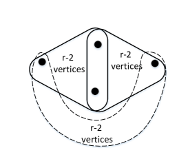
Figure 3: $(2r-2)$-subset in the reverse Type-$4$ switching

Firstly, by Lemma 3.4, there are

$$\biggl{[}\binom{n}{2r-2}-\binom{r}{2}m\binom{n-2}{2r-4}\biggr{]}\biggl{(}1+O\Bigl{(}\frac{r^{6}mn\log(r^{-2}n)+r^{8}m^{2}}{n^{4}}\Bigr{)}\biggr{)}$$

ways to choose a $(2r-2)$-set $T$ from $[n]$ such that no two vertices belong to the same edge of $H^{\prime\prime}$. For every such $T$, there are $\frac{1}{2}\binom{2r-2}{2}\binom{2r-4}{r-2}$ ways to create a Type-$4$ cluster.

Secondly, by Lemma 3.5, there are

$$\binom{r}{2}m\binom{n-2}{2r-4}\biggl{(}1+O\Bigl{(}\frac{r^{2}n\log(r^{-2}n)+r^{4}m}{n^{2}}\Bigr{)}\biggr{)}$$

ways to choose a $(2r-2)$-set $T$ from $[n]$ such that exactly two vertices belong to the same edge of $H^{\prime\prime}$. For every such $T$, there are $\binom{2r-4}{2}\binom{2r-6}{r-3}$ ways to create a Type-$4$ cluster. Thus, we have

$$|\mathcal{S}^{\prime} (H^{\prime\prime})|$$

$$=2\binom{m-2(h_{4}-1)}{2}\biggl{[}\frac{\binom{2r-2}{2}\binom{2r-4}{r-2}}{2}\biggl{(}\binom{n}{2r-2}-\binom{r}{2}m\binom{n-2}{2r-4}\biggr{)}$$

$${\qquad}+\binom{2r-4}{2}\binom{2r-6}{r-3}\binom{r}{2}m\binom{n-2}{2r-4}\biggr{]}\biggl{(}1+O\Bigl{(}\frac{r^{6}mn\log(r^{-2}n)+r^{8}m^{2}}{n^{4}}\Bigr{)}\biggr{)}$$

$$=\binom{2r-2}{2}\binom{2r-4}{r-2}\binom{m-2(h_{4}-1)}{2}\biggl{[}\binom{n}{2r-2}-\frac{(r^{2}-r-1)}{(r-1)(2r-3)}\binom{r}{2}m\binom{n-2}{2r-4}\biggr{]}$$

$${\qquad}\times\biggl{(}1+O\Bigl{(}\frac{r^{6}mn\log(r^{-2}n)+r^{8}m^{2}}{n^{4}}\Bigr{)}\biggr{)}.\qed$$

Corollary 5.16.

With notation as above, for some $0\leq h_{4}\leq M_{4}$,
$(a)$ If $\mathcal{C}_{0,0,0,h_{4}}^{++}=\emptyset$, then $\mathcal{C}_{0,0,0,h_{4}+1}^{++}=\emptyset$.
$(b)$ Let $h_{4}^{\prime}$ be the first value of $h_{4}\leq M_{4}$ such that $\mathcal{C}_{0,0,0,h_{4}}^{++}=\emptyset$, or $h_{4}^{\prime}=M_{4}+1$ if no such value exists. Suppose that $n\to\infty$. Then uniformly for $1\leq h_{4}<h_{4}^{\prime}$,

$$\frac{|\mathcal{C}_{0,0,0,h_{4}}^{++}|}{|\mathcal{C}_{0,0,0,h_{4}-1}^{++}|} =\frac{\binom{2r-2}{2}\binom{2r-4}{r-2}\binom{m-2(h_{4}-1)}{2}\bigl{[}\binom{n}{2r-2}-\frac{(r^{2}-r-1)}{(r-1)(2r-3)}\binom{r}{2}m\binom{n-2}{2r-4}\bigr{]}}{h_{4}\bigl{[}N-\binom{r}{2}m\binom{n-2}{r-2}\bigr{]}^{2}}$$

$${\qquad}\times\biggl{(}1+O\Bigl{(}\frac{r^{6}mn\log(r^{-2}n)+r^{8}m^{2}}{n^{4}}\Bigr{)}\biggr{)}.$$

Proof.

This is proved in the same way as Corollary 5.4. ∎

6 Analysis of switchings

In this section, we estimate the sum

$$\sum_{h_{4}=0}^{M_{4}}\sum_{h_{3}=0}^{M_{3}}\sum_{h_{2}=0}^{M_{2}}\sum_{h_{1}=0}^{M_{1}}\frac{|\mathcal{C}_{h_{1},h_{2},h_{3},h_{4}}^{++}|}{|\mathcal{C}_{0,0,0,0}^{++}|}$$

to finish the proof of the case $r^{-2}n\leq m=o(r^{-3}n^{\frac{3}{2}})$ in accordance with Remark 4.5. We will need the following summation lemmas from [8], and state them here for completeness.

Lemma 6.1 ([8], Corollary 4.3).

Let $K$, $N$ be integers with $N\geq 2$ and $0\leq K\leq N$. Suppose that there are real numbers $\delta_{i}$ for $1\leq i\leq N$, and $\gamma_{i}$ for $0\leq i\leq K$ such that $\sum_{j=1}^{i}|\delta_{j}|\leq\sum_{j=0}^{K}\gamma_{j}[i]_{j}<\frac{1}{5}$ for $1\leq i\leq N$. Let real numbers $A(i)$, $B(i)$ be given such that $A(i)\geq 0$ and $1-(i-1)B(i)\geq 0$. Define $A_{1}=\min_{i=1}^{N}A(i)$, $A_{2}=\max_{i=1}^{N}A(i)$, $B_{1}=\min_{i=1}^{N}B(i)$ and $B_{2}=\max_{i=1}^{N}B(i)$. Also suppose all $A\in[A_{1},A_{2}]$, $B\in[B_{1},B_{2}]$ and $c$ be real numbers such that $c>2e$, $0\leq Ac<N-K+1$ and $|BN|<1$. Define $n_{0},n_{1},\ldots,n_{N}$ by $n_{0}=1$ and

$$\frac{n_{i}}{n_{i-1}}=\frac{A(i)}{i}\bigl{(}1-(i-1)B(i)\bigr{)}\bigl{(}1+\delta_{i}\bigr{)}$$

for $1\leq i\leq N$, with the following interpretation: if $A(i)=0$ or $1-(i-1)B(i)=0$, then $n_{j}=0$ for $i\leq j\leq N$. Then

$$\Sigma_{1}\leq\sum_{i=0}^{N}n_{i}\leq\Sigma_{2},$$

where

$$\Sigma_{1} =\exp\Bigl{[}A_{1}-\lower 0.6458pt\hbox{\large$\textstyle\frac{1}{2}$}A_{1}^{2}B_{2}-4\sum_{j=0}^{K}\gamma_{j}\bigl{(}3A_{1}\bigr{)}^{j}\Bigr{]}-\lower 0.6458pt\hbox{\large$\textstyle\frac{1}{4}$}\bigl{(}2e/c\bigr{)}^{N},$$

$$\Sigma_{2} =\exp\Bigl{[}A_{2}-\lower 0.6458pt\hbox{\large$\textstyle\frac{1}{2}$}A_{2}^{2}B_{1}+\lower 0.6458pt\hbox{\large$\textstyle\frac{1}{2}$}A_{2}^{3}B_{1}^{2}+4\sum_{j=0}^{K}\gamma_{j}\bigl{(}3A_{2}\bigr{)}^{j}\Bigr{]}+\lower 0.6458pt\hbox{\large$\textstyle\frac{1}{4}$}\bigl{(}2e/c\bigr{)}^{N}.$$

Lemma 6.2 ([8], Corollary 4.5).

Let $N\geq 2$ be an integer, and for $1\leq i\leq N$, let real numbers $A(i)$, $B(i)$ be given such that $A(i)\geq 0$ and $1-(i-1)B(i)\geq 0$. Define $A_{1}=\min_{i=1}^{N}A(i)$, $A_{2}=\max_{i=1}^{N}A(i)$, $C_{1}=\min_{i=1}^{N}A(i)B(i)$ and $C_{2}=\max_{i=1}^{N}A(i)B(i)$. Suppose that there exists a real number $\hat{c}$ with $0<\hat{c}<\frac{1}{3}$ such that $\max\{A/N,|C|\}\leq\hat{c}$ for all $A\in[A_{1},A_{2}]$, $C\in[C_{1},C_{2}]$. Define $n_{0}$, $n_{1}$, $\ldots$, $n_{N}$ by $n_{0}=1$ and

$$\frac{n_{i}}{n_{i-1}}=\frac{A(i)}{i}\left(1-(i-1)B(i)\right)$$

for $1\leq i\leq N$, with the following interpretation: if $A(i)=0$ or $1-(i-1)B(i)=0$, then $n_{j}=0$ for $i\leq j\leq N$. Then

$$\Sigma_{1}\leq\sum_{i=0}^{N}n_{i}\leq\Sigma_{2},$$

where

$$\Sigma_{1} =\exp\Bigl{[}A_{1}-\lower 0.6458pt\hbox{\large$\textstyle\frac{1}{2}$}A_{1}C_{2}\Bigr{]}-\bigl{(}2e\hat{c}\bigr{)}^{N},$$

$$\Sigma_{2} =\exp\Bigl{[}A_{2}-\lower 0.6458pt\hbox{\large$\textstyle\frac{1}{2}$}A_{2}C_{1}+\lower 0.6458pt\hbox{\large$\textstyle\frac{1}{2}$}A_{2}C_{1}^{2}\Bigr{]}+\bigl{(}2e\hat{c}\bigr{)}^{N}.$$

Lemma 6.3.

Assume $r^{-2}n\leq m=o(r^{-3}n^{\frac{3}{2}})$. If $\bigl{|}\mathcal{C}_{0,h_{2},h_{3},h_{4}}^{++}\bigl{|}\neq 0$, then

$$\sum_{h_{1}=0}^{M_{1}}\frac{|\mathcal{C}_{h_{1},h_{2},h_{3},h_{4}}^{++}|}{|\mathcal{C}_{0,h_{2},h_{3},h_{4}}^{++}|}=\exp\biggl{[}\frac{6\binom{3r-4}{r}\binom{r}{4}\binom{2r-4}{r-2}m^{3}\bigl{[}\binom{n}{3r-4}-\binom{r}{2}m\binom{n-2}{3r-6}\bigr{]}}{\bigl{[}N-\binom{r}{2}m\binom{n-2}{r-2}\bigr{]}^{3}}+O\Bigl{(}\frac{r^{6}m^{2}}{n^{3}}\Bigr{)}\biggr{]}.$$

Proof.

Let $h_{1}^{\prime}=h_{1}^{\prime}(h_{2},h_{3},h_{4})$ be the first value of $h_{1}\leq M_{1}$ such that $\mathcal{C}_{h_{1},h_{2},h_{3},h_{4}}^{++}=\emptyset$, or $h_{1}^{\prime}=M_{1}+1$ if no such value exists, which is defined in Corollary 5.4 $(b)$. Since $|\mathcal{C}_{0,h_{2},h_{3},h_{4}}^{++}|\neq 0$, we know $h_{1}^{\prime}\geq 1$. Define $n_{1,0},\ldots,n_{1,M_{1}}$ by $n_{1,0}=1$,

$$n_{1,h_{1}}=\frac{|\mathcal{C}_{h_{1},h_{2},h_{3},h_{4}}^{++}|}{|\mathcal{C}_{0,h_{2},h_{3},h_{4}}^{++}|}$$

for $1\leq h_{1}<h_{1}^{\prime}$ and $n_{1,h_{1}}=0$ for $h_{1}^{\prime}\leq h_{1}\leq M_{1}$. Note that

$$\binom{m-3(h_{1}-1)-3(h_{2}+h_{3})-2h_{4}}{3}$$

$${\qquad}=\frac{m^{3}}{6}\biggl{(}1+O\Bigl{(}\frac{r^{4}m}{n^{2}}+\frac{\log(r^{-2}n)}{m}\Bigr{)}\biggr{)}\Bigl{(}1-(h_{1}-1)\frac{9}{m}\Bigr{)}.$$

By Corollary 5.4 $(b)$, we have for $1\leq h_{1}<h_{1}^{\prime}$,

$$\begin{split}\frac{|\mathcal{C}_{h_{1},h_{2},h_{3},h_{4}}^{++}|}{|\mathcal{C}_{0,h_{2},h_{3},h_{4}}^{++}|}&=\frac{1}{h_{1}}\frac{|\mathcal{C}_{h_{1}-1,h_{2},h_{3},h_{4}}^{++}|}{|\mathcal{C}_{0,h_{2},h_{3},h_{4}}^{++}|}\frac{6\binom{3r-4}{r}\binom{r}{4}\binom{2r-4}{r-2}m^{3}\bigl{[}\binom{n}{3r-4}-\binom{r}{2}m\binom{n-2}{3r-6}\bigr{]}}{\bigl{[}N-\binom{r}{2}m\binom{n-2}{r-2}\bigr{]}^{3}}\\ &{\qquad}\times\biggl{(}1+O\biggl{(}\frac{r^{4}m}{n^{2}}+\frac{\log(r^{-2}n)}{m}+\frac{r^{6}mn\log(r^{-2}n)+r^{8}m^{2}}{n^{4}}\biggr{)}\biggr{)}\\ &{\qquad}\times\Bigl{(}1-(h_{1}-1)\frac{9}{m}\Bigr{)}.\end{split}$$ (6.1)

Define

$$A(1,h_{1}) =\frac{6\binom{3r-4}{r}\binom{r}{4}\binom{2r-4}{r-2}m^{3}\bigl{[}\binom{n}{3r-4}-\binom{r}{2}m\binom{n-2}{3r-6}\bigr{]}}{\bigl{[}N-\binom{r}{2}m\binom{n-2}{r-2}\bigr{]}^{3}}$$

$${\qquad}\times\biggl{(}1+O\biggl{(}\frac{r^{4}m}{n^{2}}+\frac{\log(r^{-2}n)}{m}+\frac{r^{6}mn\log(r^{-2}n)+r^{8}m^{2}}{n^{4}}\biggr{)}\biggr{)}$$

for $1\leq h_{1}<h_{1}^{\prime}$ and $A(1,h_{1})=0$ for $h_{1}^{\prime}\leq h_{1}\leq M_{1}$, and $B(1,h_{1})=\frac{9}{m}$ for $1\leq h_{1}\leq M_{1}$. Let $A_{1,1}=\min_{h_{1}=1}^{M_{1}}A(1,h_{1})$, $A_{1,2}=\max_{h_{1}=1}^{M_{1}}A(1,h_{1})$, $C_{1,1}=\min_{h_{1}=1}^{M_{1}}A(1,h_{1})B(1,h_{1})$ and $C_{1,2}=\max_{h_{1}=1}^{M_{1}}A(1,h_{1})B(1,h_{1})$. By (6.1) we have

$$\frac{n_{1,h_{1}}}{n_{1,h_{1}-1}}=\frac{A(1,h_{1})}{h_{1}}\bigl{(}1-(h_{1}-1)B(1,h_{1})\bigr{)}.$$

Let $\hat{c}=\frac{1}{3^{4}}$, then we have $\max\bigl{\{}A/M_{1},|C|\bigr{\}}\leq\hat{c}<\frac{1}{3}$ for all $A\in[A_{1,1},A_{1,2}]$, $C\in[C_{1,1},C_{1,2}]$. Therefore, Lemma 6.2 applies and we obtain

$$\sum_{h_{1}=0}^{M_{1}} \frac{|\mathcal{C}_{h_{1},h_{2},h_{3},h_{4}}^{++}|}{|\mathcal{C}_{0,h_{2},h_{3},h_{4}}^{++}|}$$

$$=\exp\biggl{[}\frac{6\binom{3r-4}{r}\binom{r}{4}\binom{2r-4}{r-2}m^{3}\bigl{[}\binom{n}{3r-4}-\binom{r}{2}m\binom{n-2}{3r-6}\bigr{]}}{\bigl{[}N-\binom{r}{2}m\binom{n-2}{r-2}\bigr{]}^{3}}$$

$${\qquad}+O\biggl{(}\frac{r^{12}m^{4}}{n^{6}}+\frac{r^{8}m^{2}\log(r^{-2}n)}{n^{4}}+\frac{r^{14}m^{4}n\log(r^{-2}n)+r^{16}m^{5}}{n^{8}}\biggr{)}\biggr{]}+O\Bigl{(}\Bigl{(}\frac{2e}{3^{4}}\Bigr{)}^{M_{1}}\Bigr{)}.$$

Note that $O\bigl{(}\frac{r^{12}m^{4}}{n^{6}}+\frac{r^{8}m^{2}\log(r^{-2}n)}{n^{4}}+\frac{r^{14}m^{4}n\log(r^{-2}n)+r^{16}m^{5}}{n^{8}}\bigr{)}=O\bigl{(}\frac{r^{6}m^{2}}{n^{3}}\bigr{)}$ and $O\bigl{(}\bigl{(}\frac{2e}{3^{4}}\bigr{)}^{M_{1}}\bigr{)}=O\bigl{(}\frac{r^{6}}{n^{3}}\bigr{)}$ as $r^{-2}n\leq m=o(r^{-3}n^{\frac{3}{2}})$, which gives the expression in the lemma. ∎

Note that the values of $h_{2},h_{3},h_{4}$ disappear into the error term of Lemma 6.3. This means that Type-$2$ switchings can be analysed in the same way using Corollary 5.8. The values of $h_{3}$ and $h_{4}$ again disappear into the error term, so we can analyse Type-$3$ switchings in the same way using Corollary 5.12. As these two analyses are essentially the same as Lemma 6.3, we will just state the results without proof.

Lemma 6.4.

Assume $r^{-2}n\leq m=o(r^{-3}n^{\frac{3}{2}})$. If $|\mathcal{C}_{0,0,h_{3},h_{4}}^{++}|\neq 0$, then

$$\sum_{h_{2}=0}^{M_{2}} \sum_{h_{1}=0}^{M_{1}}\frac{|\mathcal{C}_{h_{1},h_{2},h_{3},h_{4}}^{++}|}{|\mathcal{C}_{0,0,h_{3},h_{4}}^{++}|}$$

$${}=\exp\biggl{[}\frac{\bigl{[}6\binom{r}{4}+3\binom{r}{3}\bigr{]}\binom{3r-4}{r}\binom{2r-4}{r-2}m^{3}\bigl{[}\binom{n}{3r-4}-\binom{r}{2}m\binom{n-2}{3r-6}\bigr{]}}{\bigl{[}N-\binom{r}{2}m\binom{n-2}{r-2}\bigr{]}^{3}}+O\Bigl{(}\frac{r^{6}m^{2}}{n^{3}}\Bigr{)}\biggr{]}.\quad\qed$$

Lemma 6.5.

Assume $r^{-2}n\leq m=o(r^{-3}n^{\frac{3}{2}})$. If $|\mathcal{C}_{0,0,0,h_{4}}^{++}|\neq 0$, then

$$\sum_{h_{3}=0}^{M_{3}} \sum_{h_{2}=0}^{M_{2}}\sum_{h_{1}=0}^{M_{1}}\frac{|\mathcal{C}_{h_{1},h_{2},h_{3},h_{4}}^{++}|}{|\mathcal{C}_{0,0,0,h_{4}}^{++}|}$$

$$=\exp\biggl{[}\frac{\bigl{[}6\binom{r}{4}+3\binom{r}{3}+\frac{1}{6}\binom{r}{2}\bigr{]}\binom{3r-4}{r}\binom{2r-4}{r-2}m^{3}\bigl{[}\binom{n}{3r-4}-\binom{r}{2}m\binom{n-2}{3r-6}\bigr{]}}{\bigl{[}N-\binom{r}{2}m\binom{n-2}{r-2}\bigr{]}^{3}}+O\Bigl{(}\frac{r^{6}m^{2}}{n^{3}}\Bigr{)}\biggr{]}.\qed$$

Lemma 6.6.

Assume $r^{-2}n\leq m=o(r^{-3}n^{\frac{3}{2}})$. Then

$$\sum_{h_{4}=0}^{M_{4}}\sum_{h_{3}=0}^{M_{3}} \sum_{h_{2}=0}^{M_{2}}\sum_{h_{1}=0}^{M_{1}}\frac{|\mathcal{C}_{h_{1},h_{2},h_{3},h_{4}}^{++}|}{|\mathcal{C}_{0,0,0,0}^{++}|}$$

$$=\exp\biggl{[}\frac{\binom{2r-2}{2}\binom{2r-4}{r-2}m^{2}\bigl{[}\binom{n}{2r-2}-\frac{(r^{2}-r-1)}{(r-1)(2r-3)}\binom{r}{2}m\binom{n-2}{2r-4}\bigr{]}}{2\bigl{[}N-\binom{r}{2}m\binom{n-2}{r-2}\bigr{]}^{2}}$$

$${\qquad}-\frac{\binom{2r-2}{2}^{2}\binom{2r-4}{r-2}^{2}m^{3}\bigl{[}\binom{n}{2r-2}-\frac{(r^{2}-r-1)}{(r-1)(2r-3)}\binom{r}{2}m\binom{n-2}{2r-4}\bigr{]}^{2}}{2\bigl{[}N-\binom{r}{2}m\binom{n-2}{r-2}\bigr{]}^{4}}$$

$${\qquad}+\frac{\bigl{[}6\binom{r}{4}+3\binom{r}{3}+\frac{1}{6}\binom{r}{2}\bigr{]}\binom{3r-4}{r}\binom{2r-4}{r-2}m^{3}\bigl{[}\binom{n}{3r-4}-\binom{r}{2}m\binom{n-2}{3r-6}\bigr{]}}{\bigl{[}N-\binom{r}{2}m\binom{n-2}{r-2}\bigr{]}^{3}}+O\Bigl{(}\frac{r^{6}m^{2}}{n^{3}}\Bigr{)}\biggr{]}.$$

Proof.

Due to the larger number of Type-$4$ clusters, Lemma 6.2 is not accurate enough and we must use Lemma 6.1. Let $h_{4}^{\prime}$ be the first value of $h_{4}\leq M_{4}$ such that $\mathcal{C}_{0,0,0,h_{4}}^{++}=\emptyset$ or $h_{4}^{\prime}=M_{4}+1$ if no such value exists, which is defined in Corollary 5.16 $(b)$. Note that

$$\sum_{h_{4}=0}^{M_{4}}\sum_{h_{3}=0}^{M_{3}}\sum_{h_{2}=0}^{M_{2}}\sum_{h_{1}=0}^{M_{1}}\frac{|\mathcal{C}_{h_{1},h_{2},h_{3},h_{4}}^{++}|}{|\mathcal{C}_{0,0,0,0}^{++}|}=\sum_{h_{4}=0}^{h_{4}^{\prime}-1}\biggl{(}\frac{|\mathcal{C}_{0,0,0,h_{4}}^{++}|}{|\mathcal{C}_{0,0,0,0}^{++}|}\sum_{h_{3}=0}^{M_{3}}\sum_{h_{2}=0}^{M_{2}}\sum_{h_{1}=0}^{M_{1}}\frac{|\mathcal{C}_{h_{1},h_{2},h_{3},h_{4}}^{++}|}{|\mathcal{C}_{0,0,0,h_{4}}^{++}|}\biggr{)}.$$

Thus, by the definition of $h_{4}^{\prime}$, $|\mathcal{C}_{0,0,0,h_{4}}^{++}|\neq 0$ for $0\leq h_{4}<h_{4}^{\prime}$. By Lemma 6.5, we have

$$\sum_{h_{4}=0}^{M_{4}} \sum_{h_{3}=0}^{M_{3}}\sum_{h_{2}=0}^{M_{2}}\sum_{h_{1}=0}^{M_{1}}\frac{|\mathcal{C}_{h_{1},h_{2},h_{3},h_{4}}^{++}|}{|\mathcal{C}_{0,0,0,0}^{++}|}$$

$$=\exp\biggl{[}\frac{\bigl{[}6\binom{r}{4}+3\binom{r}{3}+\frac{1}{6}\binom{r}{2}\bigr{]}\binom{3r-4}{r}\binom{2r-4}{r-2}m^{3}\bigl{[}\binom{n}{3r-4}-\binom{r}{2}m\binom{n-2}{3r-6}\bigr{]}}{\bigl{[}N-\binom{r}{2}m\binom{n-2}{r-2}\bigr{]}^{3}}+O\Bigl{(}\frac{r^{6}m^{2}}{n^{3}}\Bigr{)}\biggr{]}$$

$${\qquad}\times\sum_{h_{4}=0}^{h_{4}^{\prime}-1}\frac{|\mathcal{C}_{0,0,0,h_{4}}^{++}|}{|\mathcal{C}_{0,0,0,0}^{++}|}.$$

By Remark 4.3 and Remark 4.4, we have $|\mathcal{C}_{0,0,0,0}^{++}|\neq 0$. Define $n_{4,0},\ldots,n_{4,M_{4}}$ by $n_{4,0}=1$,

$$n_{4,h_{4}}=\frac{|\mathcal{C}_{0,0,0,h_{4}}^{++}|}{|\mathcal{C}_{0,0,0,0}^{++}|}$$

for $1\leq h_{4}<h_{4}^{\prime}$ and $n_{4,h_{4}}=0$ for $h_{4}^{\prime}\leq h_{4}\leq M_{4}$, where $M_{4}$ is shown in the equation (3.1). Note that as $n\to\infty$, $r^{-2}n\leq m=o(r^{-3}n^{\frac{3}{2}})$ and $h_{4}\leq M_{4}$,

$$\binom{m-2(h_{4}-1)}{2}=\frac{m^{2}}{2}\biggl{(}1+O\Bigl{(}\frac{r^{8}m^{2}}{n^{4}}+\frac{1}{m}\Bigr{)}\biggr{)}\Bigl{(}1-(h_{4}-1)\frac{4}{m}\Bigr{)}.$$

By Corollary 5.16 $(b)$, we have for $1\leq h_{4}\leq h_{4}^{\prime}$,

$$\begin{split}\frac{|\mathcal{C}_{0,0,0,h_{4}}^{++}|}{|\mathcal{C}_{0,0,0,0}^{++}|}&=\frac{1}{h_{4}}\frac{|\mathcal{C}_{0,0,0,h_{4}-1}^{++}|}{|\mathcal{C}_{0,0,0,0}^{++}|}\frac{\binom{2r-2}{2}\binom{2r-4}{r-2}m^{2}\bigl{[}\binom{n}{2r-2}-\frac{(r^{2}-r-1)}{(r-1)(2r-3)}\binom{r}{2}m\binom{n-2}{2r-4}\bigr{]}}{2\bigl{[}N-\binom{r}{2}m\binom{n-2}{r-2}\bigr{]}^{2}}\\ &{}\times\biggl{(}1+O\biggl{(}\frac{r^{8}m^{2}}{n^{4}}+\frac{1}{m}+\frac{r^{6}mn\log(r^{-2}n)+r^{8}m^{2}}{n^{4}}\biggr{)}\biggr{)}\Bigl{(}1-(h_{4}-1)\frac{4}{m}\Bigr{)}.\end{split}$$ (6.2)

Define

$$A(4,h_{4}) =\frac{\binom{2r-2}{2}\binom{2r-4}{r-2}m^{2}\bigl{[}\binom{n}{2r-2}-\frac{(r^{2}-r-1)}{(r-1)(2r-3)}\binom{r}{2}m\binom{n-2}{2r-4}\bigr{]}}{2\bigl{[}N-\binom{r}{2}m\binom{n-2}{r-2}\bigr{]}^{2}}$$

$${\qquad}\times\biggl{(}1+O\biggl{(}\frac{r^{8}m^{2}}{n^{4}}+\frac{1}{m}+\frac{r^{6}mn\log(r^{-2}n)+r^{8}m^{2}}{n^{4}}\biggr{)}\biggr{)}$$

for $1\leq h_{4}<h_{4}^{\prime}$ and $A(4,h_{4})=0$ for $h_{4}^{\prime}\leq h_{4}\leq M_{4}$,

$$B(4,h_{4})=\frac{4}{m}\text{~{}~{}and~{}~{}}\delta_{h_{4}}=0$$

for $1\leq h_{4}\leq M_{4}$. Define $K=1$, $c=3^{4}$ and $\gamma_{j}=0$ for $0\leq j\leq K$. By (6.2), we further have

$$\frac{n_{4,h_{4}}}{n_{4,h_{4}-1}}=\frac{A(4,h_{4})}{h_{4}}\bigl{(}1-(h_{4}-1)B(4,h_{4})\bigr{)}.$$

Let $A_{4,1}=\min_{h_{4}=1}^{M_{4}}A(4,h_{4})$, $A_{4,2}=\max_{h_{4}=1}^{M_{4}}A(4,h_{4})$, $B_{4,1}=\min_{h_{4}=1}^{M_{4}}B(4,h_{4})=\frac{4}{m}$, $B_{4,2}=\max_{h_{4}=1}^{M_{4}}B(4,h_{4})=\frac{4}{m}$. Since $Ac\leq\frac{3^{4}r^{4}m^{2}}{4n^{2}}<M_{4}-K+1$ and $BM_{4}=o(1)<1$ for all $A\in[A_{4,1},A_{4,2}]$ and $B\in[B_{4,1},B_{4,2}]$, Lemma 6.1 applies and we obtain

$$\sum_{h_{4}=0}^{M_{4}}\frac{|\mathcal{C}_{0,0,0,h_{4}}^{++}|}{|\mathcal{C}_{0,0,0,0}^{++}|} =\exp\biggl{[}\frac{\binom{2r-2}{2}\binom{2r-4}{r-2}m^{2}\bigl{[}\binom{n}{2r-2}-\frac{(r^{2}-r-1)}{(r-1)(2r-3)}\binom{r}{2}m\binom{n-2}{2r-4}\bigr{]}}{2\bigl{[}N-\binom{r}{2}m\binom{n-2}{r-2}\bigr{]}^{2}}$$

$${\qquad}-\frac{\binom{2r-2}{2}^{2}\binom{2r-4}{r-2}^{2}m^{3}\bigl{[}\binom{n}{2r-2}-\frac{(r^{2}-r-1)}{(r-1)(2r-3)}\binom{r}{2}m\binom{n-2}{2r-4}\bigr{]}^{2}}{2\bigl{[}N-\binom{r}{2}m\binom{n-2}{r-2}\bigr{]}^{4}}$$

$${\qquad}+O\biggl{(}\frac{r^{12}m^{4}}{n^{6}}+\frac{r^{4}m}{n^{2}}+\frac{r^{10}m^{3}n\log(r^{-2}n)+r^{12}m^{4}}{n^{6}}\biggr{)}\biggr{]}+O\Bigl{(}\Bigl{(}\frac{2e}{3^{4}}\Bigr{)}^{M_{4}}\Bigr{)}.$$

Note that $O\bigl{(}\frac{r^{12}m^{4}}{n^{6}}+\frac{r^{4}m}{n^{2}}+\frac{r^{10}m^{3}n\log(r^{-2}n)+r^{12}m^{4}}{n^{6}}\bigr{)}=O\bigl{(}\frac{r^{6}m^{2}}{n^{3}}\bigr{)}$ and $O\bigl{(}\bigl{(}\frac{2e}{3^{4}}\bigr{)}^{M_{3}}\bigr{)}=O\bigl{(}\frac{r^{6}}{n^{3}}\bigr{)}$, which further leads to

$$\sum_{h_{4}=0}^{M_{4}}\frac{|\mathcal{C}_{0,0,0,h_{4}}^{++}|}{|\mathcal{C}_{0,0,0,0}^{++}|} =\exp\biggl{[}\frac{\binom{2r-2}{2}\binom{2r-4}{r-2}m^{2}\bigl{[}\binom{n}{2r-2}-\frac{(r^{2}-r-1)}{(r-1)(2r-3)}\binom{r}{2}m\binom{n-2}{2r-4}\bigr{]}}{2\bigl{[}N-\binom{r}{2}m\binom{n-2}{r-2}\bigr{]}^{2}}$$

$${\qquad}-\frac{\binom{2r-2}{2}^{2}\binom{2r-4}{r-2}^{2}m^{3}\bigl{[}\binom{n}{2r-2}-\frac{(r^{2}-r-1)}{(r-1)(2r-3)}\binom{r}{2}m\binom{n-2}{2r-4}\bigr{]}^{2}}{2\bigl{[}N-\binom{r}{2}m\binom{n-2}{r-2}\bigr{]}^{4}}+O\Bigl{(}\frac{r^{6}m^{2}}{n^{3}}\Bigr{)}\biggr{]}.$$

This gives the expression in the lemma statement. ∎

7 The case $\log\,(r^{-2}n)\leq m=O(r^{-2}n)$

We consider the case $\log(r^{-2}n)\leq m=O(r^{-2}n)$ in Theorem 1.1. Recall that these inequalities imply $r=o(n^{\frac{1}{2}})$. Define

$$\begin{split}M_{0}^{*}&=\Bigl{\lceil}\log(r^{-2}n)\Bigr{\rceil},\\ M_{0}&=\Bigl{\lceil}\log(r^{-2}n)\Bigr{\rceil}+2,\\ M_{4}&=\Bigl{\lceil}\log(r^{-2}n)\Bigr{\rceil}.\end{split}$$ (7.1)

Let $\mathcal{H}_{r}^{+}(n,m)\subseteq\mathcal{H}_{r}(n,m)$ be the set of $r$-graphs $H$ which satisfy properties $\bf(a)$ to $\bf(e)$:

$\bf(a)$  The intersection of any two edges contains at most two vertices.

$\bf(b)$  $H$ only contains one type of cluster (Type-$4$ cluster). (This implies that any three edges involve at least $3r-3$ vertices. Thus, if there are two edges, for example $\{e_{1},e_{2}\}$, such that $|e_{1}\cup e_{2}|=2r-2$, then $|(e_{1}\cup e_{2})\cap e|\leq 1$ for any edge $e$ other than $\{e_{1},e_{2}\}$ of $H$.)

$\bf(c)$ Any two distinct Type-$4$ clusters in $H$ are vertex-disjoint. (This implies that any four edges involve at least $4r-4$ vertices.)

$\bf(d)$ There are at most $M_{4}$ Type-$4$ clusters in $H$.

$\bf(e)$ $\deg(v)\leq M_{0}$ for every vertex $v\in[n]$.

Similarly, we further define $\mathcal{H}_{r}^{++}(n,m)\subseteq\mathcal{H}_{r}^{+}(n,m)$ to be the set of $r$-graphs $H$ obtained by replacing the property $\bf(e)$ with a stronger constraint

$\bf(e^{*})$ $\deg(v)\leq M_{0}^{*}$ for every vertex $v\in[n]$.

Remark 7.1.

From property $\bf(e)$, it easily follows that

$$\sum_{v\in[n]}\binom{\deg(v)}{2}=O\Bigl{(}M_{0}\sum_{v\in[n]}\deg_{0}(v)\Bigr{)}=O\Bigl{(}rm\log(r^{-2}n)\Bigr{)}$$

for $H\in\mathcal{H}_{r}^{+}(n,m)$.

Similarly to Section 3, we find that the number of $r$-graphs in $\mathcal{H}_{r}(n,m)$ not satisfying the properties of $\mathcal{H}^{+}_{r}(n,m)$ and $\mathcal{H}^{++}_{r}(n,m)$ is quite small.

Theorem 7.2.

Assume that $\log(r^{-2}n)\leq m=O(r^{-2}n)$ and $n\to\infty$. Then

$$\frac{|\mathcal{H}^{+}_{r}(n,m)|}{|\mathcal{H}_{r}(n,m)|}=1-O\Bigl{(}\frac{r^{6}m^{2}}{n^{3}}\Bigr{)},\quad\frac{|\mathcal{H}^{++}_{r}(n,m)|}{|\mathcal{H}_{r}(n,m)|}=1-O\Bigl{(}\frac{r^{6}m^{2}}{n^{3}}\Bigr{)}.$$

Proof.

The proof is much the same as that of Theorem 3.2, so we will omit the proofs for $\bf(a)$–$\bf(d)$.

To prove property $\bf(e^{*})$, define $d=M_{0}^{*}+1$. The expected number of sets consisting of a vertex $v$ and $d$ edges that include $v$ is

$$n\binom{n-1}{r-1}^{d}\frac{1}{d!}\Bigl{(}\frac{m}{N}\Bigr{)}^{d}=O\Bigl{(}n\Bigl{(}\frac{rem}{dn}\Bigr{)}^{d}\Bigr{)}=O\Bigl{(}n\Bigl{(}\frac{e}{rd}\Bigr{)}^{d}\Bigr{)}=O\Bigl{(}\frac{r^{6}}{n^{3}}\Bigr{)},$$

where the second equality is true because $d!\geq\bigl{(}\frac{d}{e}\bigr{)}^{d}$ and $m=O(r^{-2}n)$, and the last equality is true because of the choice $d>\log(r^{-2}n)$. ∎

Remark 7.3.

Let $\mathcal{C}_{h_{4}}^{+}$ (resp. $\mathcal{C}_{h_{4}}^{++}$) be the set of $r$-graphs $H\in\mathcal{H}_{r}^{+}(n,m)$ (resp. $H\in\mathcal{H}_{r}^{++}(n,m)$) with exactly $h_{4}$ Type-$4$ clusters. Then, by Theorem 7.2,

$$|\mathcal{H}_{r}^{+}(n,m)|=\sum_{h_{4}=0}^{M_{4}}|\mathcal{C}_{h_{4}}^{+}|,\quad|\mathcal{H}_{r}^{++}(n,m)|=\sum_{h_{4}=0}^{M_{4}}|\mathcal{C}_{h_{4}}^{++}|.$$

By the same discussion as in Section 4, we also have

$$|\mathcal{C}_{0}^{++}|=\Bigl{(}1-O\Bigl{(}\frac{r^{6}}{n^{3}}\Bigr{)}\Bigr{)}|\mathcal{L}_{r}(n,m)|\quad\text{and}\quad|\mathcal{C}_{h_{4}}^{++}|=\Bigl{(}1-O\Bigl{(}\frac{r^{6}}{n^{3}}\Bigr{)}\Bigr{)}|\mathcal{C}_{h_{4}}^{+}|.$$

We also have $|\mathcal{L}_{r}(n,m)|\neq 0$ and $|\mathcal{C}_{0}^{++}|\neq 0$. Thus,

$$\frac{1}{\mathbb{P}_{r}(n,m)}=\sum_{h_{4}=0}^{M_{4}}\frac{|\mathcal{C}_{h_{4}}^{++}|}{|\mathcal{L}_{r}(n,m)|}\Bigl{(}1-O\Bigl{(}\frac{r^{6}m^{2}}{n^{3}}\Bigr{)}\Bigr{)}=\sum_{h_{4}=0}^{M_{4}}\frac{|\mathcal{C}_{h_{4}}^{++}|}{|\mathcal{C}_{0}^{++}|}\Bigl{(}1-O\Bigl{(}\frac{r^{6}m^{2}}{n^{3}}\Bigr{)}\Bigr{)}.$$

By Remark 7.1 and the same arguments as used for Lemma 3.4 and Corollary 5.4, we also have the following two lemmas.

Lemma 7.4.

Assume $\log(r^{-2}n)\leq m=O(r^{-2}n)$. Let $H\in\mathcal{H}_{r}^{+}(n,m-\xi)$ and let $N_{t}$ be the set of $t$-sets of $[n]$ of which no two vertices belong to the same edge of $H$, where $r\leq t\leq 2r-2$ and $\xi=O(1)$. Then

$$|N_{t}|=\biggl{[}\binom{n}{t}-\binom{r}{2}m\binom{n-2}{t-2}\biggr{]}\biggl{(}1+O\Bigl{(}\frac{r^{4}}{n^{2}}+\frac{r^{6}m\log(r^{-2}n)}{n^{3}}\Bigr{)}\biggr{)}.$$

Lemma 7.5.

Assume $\log(r^{-2}n)\leq m=O(r^{-2}n)$. With notation as above,
$(a)$ If $\mathcal{C}_{h_{4}}^{++}=\emptyset$, then $\mathcal{C}_{h_{4}+1}^{++}=\emptyset$.
$(b)$ Let $h_{4}^{\prime}$ be the first value of $h_{4}\leq M_{4}$ such that $\bigl{|}\mathcal{C}_{h_{4}}^{++}\bigl{|}=0$, or $h_{4}^{\prime}=M_{4}+1$ if no such value exists. Suppose that $n\to\infty$, then uniformly for $1\leq h_{4}<h_{4}^{\prime}$,

$$\frac{|\mathcal{C}_{h_{4}}^{++}|}{|\mathcal{C}_{h_{4}-1}^{++}|} =\frac{\binom{2r-2}{2}\binom{2r-4}{r-2}\binom{m-2(h_{4}-1)}{2}\bigl{[}\binom{n}{2r-2}-\binom{r}{2}m\binom{n-2}{2r-4}\bigr{]}}{h_{4}\bigl{[}N-\binom{r}{2}m\binom{n-2}{r-2}\bigr{]}^{2}}$$

$${\qquad}\times\biggl{(}1+O\Bigl{(}\frac{r^{4}}{n^{2}}+\frac{r^{6}m\log(r^{-2}n)}{n^{3}}\Bigr{)}\biggr{)}.$$

Lemma 7.6.

Assume $\log(r^{-2}n)\leq m=O(r^{-2}n)$. Then

$$\sum_{h_{4}=0}^{M_{4}}\frac{|\mathcal{C}_{h_{4}}^{++}|}{|\mathcal{C}_{0}^{++}|}=\exp\biggl{[}\frac{[m]_{2}\binom{2r-2}{2}\binom{2r-4}{r-2}\bigl{[}\binom{n}{2r-2}-\binom{r}{2}m\binom{n-2}{2r-4}\bigr{]}}{2\bigl{[}N-\binom{r}{2}m\binom{n-2}{r-2}\bigr{]}^{2}}+O\Bigl{(}\frac{r^{6}m^{2}}{n^{3}}\Bigr{)}\biggr{]}.$$

Proof.

Let $h_{4}^{\prime}$ be the first value of $h_{4}\leq M_{4}$ such that $|\mathcal{C}_{h_{4}}^{++}|=0$ or $h_{4}^{\prime}=M_{4}+1$ if no such value exists, which is defined in Lemma 7.4. By Remark 7.3, we have $|\mathcal{C}_{0}^{++}|\neq 0$. Define $n_{0},\ldots,n_{M_{4}}$ by $n_{0}=1$,

$$n_{h_{4}}=\frac{|\mathcal{C}_{h_{4}}^{++}|}{|\mathcal{C}_{0}^{++}|}$$

for $1\leq h_{4}<h_{4}^{\prime}$ and $n_{h_{4}}=0$ for $h_{4}^{\prime}\leq h_{4}\leq M_{4}$, where $M_{4}$ is shown in (7.1).

Note that

$$\binom{m-2(h_{4}-1)}{2}=\frac{[m]_{2}}{2}\Bigl{(}1-(h_{4}-1)\frac{4m-4h_{4}+2}{m(m-1)}\Bigr{)}.$$

By Lemma 7.4, for $1\leq h_{4}\leq h_{4}^{\prime}$, we have

$$\begin{split}\frac{|\mathcal{C}_{h_{4}}^{++}|}{|\mathcal{C}_{0}^{++}|}&=\frac{1}{h_{4}}\frac{|\mathcal{C}_{h_{4}-1}^{++}|}{|\mathcal{C}_{0}^{++}|}\frac{[m]_{2}\binom{2r-2}{2}\binom{2r-4}{r-2}\bigl{[}\binom{n}{2r-2}-\binom{r}{2}m\binom{n-2}{2r-4}\bigr{]}}{2\bigl{[}N-\binom{r}{2}m\binom{n-2}{r-2}\bigr{]}^{2}}\\ &{\qquad}\times\biggl{(}1+O\Bigl{(}\frac{r^{4}}{n^{2}}+\frac{r^{6}m\log(r^{-2}n)}{n^{3}}\Bigr{)}\biggr{)}\biggl{(}1-(h_{4}-1)\frac{4m-4h_{4}+2}{m(m-1)}\biggr{)}.\end{split}$$ (7.2)

Define

$$A(h_{4})=\frac{[m]_{2}\binom{2r-2}{2}\binom{2r-4}{r-2}\bigl{[}\binom{n}{2r-2}-\binom{r}{2}m\binom{n-2}{2r-4}\bigr{]}}{2\bigl{[}N-\binom{r}{2}m\binom{n-2}{r-2}\bigr{]}^{2}}\biggl{(}1+O\Bigl{(}\frac{r^{4}}{n^{2}}+\frac{r^{6}m\log(r^{-2}n)}{n^{3}}\Bigr{)}\biggr{)}$$

for $1\leq h_{4}<h_{4}^{\prime}$, $A(h_{4})=0$ for $h_{4}^{\prime}\leq h_{4}\leq M_{4}$ and $B(h_{4})=\frac{4m-4h_{4}+2}{m(m-1)}=O\bigl{(}\frac{1}{m}\bigr{)}$ as $m\geq\log(r^{-2}n)$. Let $A_{1}=\min_{h_{4}=1}^{M_{4}}A(h_{4})$, $A_{2}=\max_{h_{4}=1}^{M_{4}}A(h_{4})$, $C_{1}=\min_{h_{4}=1}^{M_{4}}A(h_{4})B(h_{4})$ and $C_{2}=\max_{h_{4}=1}^{M_{4}}A(h_{4})B(h_{4})$.

We further have

$$\frac{|\mathcal{C}_{h_{4}}^{++}|}{|\mathcal{C}_{0}^{++}|}=\frac{A(h_{4})}{h_{4}}\frac{|\mathcal{C}_{h_{4}-1}^{++}|}{|\mathcal{C}_{0}^{++}|}\bigl{(}1-(h_{4}-1)B(h_{4})\bigr{)}.$$

Note that $\max\{A/M_{4},|C|\}=o(1)$ for all $A\in[A_{1},A_{2}]$ and $C\in[C_{1},C_{2}]$ as $\log(r^{-2}n)\leq m=O(r^{-2}n)$ and $h_{4}\leq M_{4}=\lceil\log(r^{-2}n)\rceil$. Let $\hat{c}=\frac{1}{2\cdot 3^{4}}$, then $\max\{A/M_{4},|C|\}\leq\hat{c}<\frac{1}{3}$. Lemma 6.2 applies to obtain

$$\sum_{h_{4}=0}^{M_{4}}\frac{|\mathcal{C}_{h_{4}}^{++}|}{|\mathcal{C}_{0}^{++}|} =\exp\biggl{[}\frac{[m]_{2}\binom{2r-2}{2}\binom{2r-4}{r-2}\bigl{[}\binom{n}{2r-2}-\binom{r}{2}m\binom{n-2}{2r-4}\bigr{]}}{2\bigl{[}N-\binom{r}{2}m\binom{n-2}{r-2}\bigr{]}^{2}}$$

$${\qquad}+O\Bigl{(}\frac{r^{8}m^{2}}{n^{4}}+\frac{r^{10}m^{3}\log(r^{-2}n)}{n^{5}}\Bigr{)}\biggr{]}+O\Bigl{(}\Bigl{(}\frac{e}{3^{4}}\Bigr{)}^{M_{4}}\Bigr{)}$$

$$=\exp\biggl{[}\frac{[m]_{2}\binom{2r-2}{2}\binom{2r-4}{r-2}\bigl{[}\binom{n}{2r-2}-\binom{r}{2}m\binom{n-2}{2r-4}\bigr{]}}{2\bigl{[}N-\binom{r}{2}m\binom{n-2}{r-2}\bigr{]}^{2}}+O\Bigl{(}\frac{r^{6}m^{2}}{n^{3}}\Bigr{)}\biggr{]},$$

where the last equality is true because $O\bigl{(}\frac{r^{8}m^{2}}{n^{4}}+\frac{r^{10}m^{3}\log(r^{-2}n)}{n^{5}}\bigr{)}=O\bigl{(}\frac{r^{6}m^{2}}{n^{3}}\bigr{)}$ as $m=O(r^{-2}n)$ and $O\bigl{(}\bigl{(}\frac{e}{3^{4}}\bigr{)}^{M_{4}}\bigr{)}=O\bigl{(}\frac{r^{6}}{n^{3}}\bigr{)}$. ∎

8 The case $1\leq m=O(\log(r^{-2}n))$

Let $\mathcal{H}_{r}^{+}(n,m)\subset\mathcal{H}_{r}(n,m)$ be the set of $r$-graphs $H$ which satisfy properties $\bf(a)$ to $\bf(d)$:

$\bf(a)$  The intersection of any two edges contains at most two vertices.

$\bf(b)$  $H$ only contains one type of cluster (Type-$4$ cluster). (This implies that any three edges involve at least $3r-3$ vertices. Thus, if there are two edges, for example $\{e_{1},e_{2}\}$, such that $|e_{1}\cup e_{2}|=2r-2$, then $|(e_{1}\cup e_{2})\cap e|\leq 1$ for any edge $e$ other than $\{e_{1},e_{2}\}$ of $H$.)

$\bf(c)$ Any two distinct Type-$4$ clusters in $H$ are vertex-disjoint. (This implies that any four edges involve at least $4r-4$ vertices.)

$\bf(d)$ There are at most two Type-$4$ clusters in $H$. (This implies that any six edges involve at least $6r-5$ vertices.)

Theorem 8.1.

Assume $1\leq m=O(\log(r^{-2}n))$ and $n\to\infty$. Then

$$\frac{|\mathcal{H}^{+}_{r}(n,m)|}{|\mathcal{H}_{r}(n,m)|}=1-O\Bigl{(}\frac{r^{6}m^{2}}{n^{3}}\Bigr{)}.$$

Proof.

Consider $H\in\mathcal{H}_{r}(n,m)$ chosen uniformly at random. We can apply Lemma 2.2 several times to show that $H$ satisfies properties $\bf(a)$-$\bf(d)$ with probability $1-O\bigl{(}\frac{r^{6}m^{2}}{n^{3}}\bigr{)}$. We only prove the property $\bf(d)$ because the proof of other conditions are exactly same with the proof in Theorem 3.2.

Applying Lemma 2.2 with $t=6$ and $\alpha=6$, the expected number of sets of six edges involving at most $6r-6$ vertices is

$$O\Bigl{(}\frac{r^{12}m^{6}}{n^{6}}\Bigr{)}=O\Bigl{(}\frac{r^{6}m^{2}}{n^{3}}\Bigr{)}$$

because $m=O(\log(r^{-2}n))$. Hence, property $\bf(d)$ holds with probability $1-O\bigl{(}\frac{r^{6}m^{2}}{n^{3}}\bigr{)}$. ∎

Remark 8.2.

By Theorem 8.1, for a nonnegative integer $h_{4}$, let $\mathcal{C}_{h_{4}}^{+}$ be the set of $r$-graphs $H\in\mathcal{H}_{r}^{+}(n,m)$ with exactly $h_{4}$ Type-$4$ clusters. Thus, we have $|\mathcal{H}_{r}^{+}(n,m)|=\sum_{h_{4}=0}^{2}|\mathcal{C}_{h_{4}}^{+}|$, $|\mathcal{C}_{0}^{+}|=|\mathcal{L}_{r}(n,m)|\neq\emptyset$ and

$$\frac{1}{\mathbb{P}_{r}(n,m)}=\sum_{h_{4}=0}^{2}\frac{|\mathcal{C}_{h_{4}}^{+}|}{|\mathcal{L}_{r}(n,m)|}\biggl{(}1-O\Bigl{(}\frac{r^{6}m^{2}}{n^{3}}\Bigr{)}\biggr{)}=\sum_{h_{4}=0}^{2}\frac{|\mathcal{C}_{h_{4}}^{+}|}{|\mathcal{C}_{0}^{+}|}\biggl{(}1-O\Bigl{(}\frac{r^{6}m^{2}}{n^{3}}\Bigr{)}\biggr{)}.$$

By arguments similar to Lemma 3.4 and Lemma 7.4, Corollary 5.4 and Lemma 7.5, we have the following two lemmas.

Lemma 8.3.

Assume $1\leq m=O(\log(r^{-2}n))$. Let $H\in\mathcal{H}_{r}^{+}(n,m-\xi)$ and $N_{t}$ be the set of $t$-sets of $[n]$ such that no two vertices belong to the same edge of $H$, where $r\leq t\leq 2r-2$ and $\xi=O(1)$ are positive integers. Suppose that $n\to\infty$. Then

$$|N_{t}|=\biggl{[}\binom{n}{t}-\binom{r}{2}m\binom{n-2}{t-2}\biggr{]}\biggl{(}1+O\Bigl{(}\frac{r^{4}}{n^{2}}\Bigr{)}\biggr{)}.$$

Lemma 8.4.

Assume $1\leq m=O(\log(r^{-2}n))$. With notation as above,
$(a)$ If $\mathcal{C}_{h_{4}}^{+}=\emptyset$, then $\mathcal{C}_{h_{4}+1}^{+}=\emptyset$.
$(b)$ Let $h_{4}^{\prime}$ be the first value of $h_{4}\leq 2$ such that $\bigl{|}\mathcal{C}_{h_{4}}^{+}\bigl{|}=0$ or $h_{4}^{\prime}=3$ if no such value exists. Suppose that $n\to\infty$, then uniformly for $1\leq h_{4}<h_{4}^{\prime}$,

$$\frac{|\mathcal{C}_{h_{4}}^{+}|}{|\mathcal{C}_{h_{4}-1}^{+}|}=\frac{\binom{2r-2}{2}\binom{2r-4}{r-2}\binom{m-2(h_{4}-1)}{2}\bigl{[}\binom{n}{2r-2}-\binom{r}{2}m\binom{n-2}{2r-4}\bigr{]}}{h_{4}\bigl{[}N-\binom{r}{2}m\binom{n-2}{r-2}\bigr{]}^{2}}\biggl{(}1+O\Bigl{(}\frac{r^{4}}{n^{2}}\Bigr{)}\biggr{)}.$$

Lemma 8.5.

Assume $1\leq m=O(\log(r^{-2}n))$. Then

$$\frac{|\mathcal{C}_{0}^{+}|+|\mathcal{C}_{1}^{+}|+|\mathcal{C}_{2}^{+}|}{|\mathcal{C}_{0}^{+}|} =\exp\biggl{[}\frac{[m]_{2}\binom{2r-2}{2}\binom{2r-4}{r-2}\bigl{[}\binom{n}{2r-2}-\binom{r}{2}m\binom{n-2}{2r-4}\bigr{]}}{2\bigl{[}N-\binom{r}{2}m\binom{n-2}{r-2}\bigr{]}^{2}}+O\Bigl{(}\frac{r^{6}m^{2}}{n^{3}}\Bigr{)}\biggr{]}.$$

Proof.

By Remark 8.2, we have $|\mathcal{C}_{0}^{+}|\neq 0$. By Lemma 8.3, we have

$$\frac{|\mathcal{C}_{1}^{+}|}{|\mathcal{C}_{0}^{+}|}=\frac{[m]_{2}\binom{2r-2}{2}\binom{2r-4}{r-2}\bigl{[}\binom{n}{2r-2}-\binom{r}{2}m\binom{n-2}{2r-4}\bigr{]}}{2\bigl{[}N-\binom{r}{2}m\binom{n-2}{r-2}\bigr{]}^{2}}\biggl{(}1+O\Bigl{(}\frac{r^{4}}{n^{2}}\Bigr{)}\biggr{)}$$

and

$$\frac{|\mathcal{C}_{2}^{+}|}{|\mathcal{C}_{1}^{+}|}=\frac{[m-1]_{2}\binom{2r-2}{2}\binom{2r-4}{r-2}\bigl{[}\binom{n}{2r-2}-\binom{r}{2}m\binom{n-2}{2r-4}\bigr{]}}{4\bigl{[}N-\binom{r}{2}m\binom{n-2}{r-2}\bigr{]}^{2}}\biggl{(}1+O\Bigl{(}\frac{r^{4}}{n^{2}}\Bigr{)}\biggr{)}.$$

Thus, we have

$$\sum_{h_{4}=0}^{2}\frac{|\mathcal{C}_{h_{4}}^{+}|}{|\mathcal{C}_{0}^{+}|} =\biggl{(}1+\frac{[m]_{2}\binom{2r-2}{2}\binom{2r-4}{r-2}\bigl{[}\binom{n}{2r-2}-\binom{r}{2}m\binom{n-2}{2r-4}\bigr{]}}{2\bigl{[}N-\binom{r}{2}m\binom{n-2}{r-2}\bigr{]}^{2}}$$

$${\qquad}+\frac{[m]_{4}\binom{2r-2}{2}^{2}\binom{2r-4}{r-2}^{2}\bigl{[}\binom{n}{2r-2}-\binom{r}{2}m\binom{n-2}{2r-4}\bigr{]}^{2}}{8\bigl{[}N-\binom{r}{2}m\binom{n-2}{r-2}\bigr{]}^{4}}+O\Bigl{(}\frac{r^{8}m^{2}}{n^{4}}\Bigr{)}\biggr{)},$$

which simplifies to the expression in the lemma statement. ∎

9 Proof of Theorem 1.2

As in the statement of Theorem 1.2, we use $m_{0}=Np$. The binomial distribution is $\operatorname{Bin}(n,p)$. Recall that $\mathbb{P}_{r}(n,m)$ denotes the probability that an $r$-graph $H\in\mathcal{H}_{r}(n,m)$ chosen uniformly at random is linear. We found an expression for $\mathbb{P}_{r}(n,m)$ in Theorem 1.1. By the law of total probability, we have

$$\mathbb{P}\bigl{[}H_{r}(n,p)\in\mathcal{L}_{r}\bigr{]}=\sum_{m=0}^{N}\mathbb{P}_{r}(n,m)\binom{N}{m}p^{m}q^{N-m}.$$ (9.1)

In the proof of Theorem 1.2, we need the following lemmas. We firstly show $\mathbb{P}_{r}(n,m)$ is decreasing in $m$ (Lemma 9.1). Some approximations will make use of the Chernoff inequality (Lemma 9.2) and the normal approximation of the binomial distribution (Lemmas 9.3 and 9.4).

Lemma 9.1.

$\mathbb{P}_{r}(n,m)$ is a non-increasing function of $m$.

Proof.

Choosing $m$ distinct edges at random gives the same distribution as choosing $m-1$ distinct edges at random and then an $m$-th edge at random distinct from the first $m-1$. So $\mathbb{P}_{r}(n,m)\leq\mathbb{P}_{r}(n,m-1)$. ∎

Lemma 9.2 ([5]).

For $X\sim\operatorname{Bin}(N,p)$ and any $0<t\leq Np$,

$$\mathbb{P}\bigl{[}|X-Np|>t\bigr{]}<2\exp\left[-t^{2}/\left(3Np\right)\right].$$

Lemma 9.3.

Let $r=r(n)\geq 3$ be an integer with $r=o(n^{\frac{1}{2}})$ and $X\sim\operatorname{Bin}(N,p)$, where $r^{-2}n\leq Np=o(r^{-3}n^{\frac{3}{2}})$. Then

$$\mathbb{P}\bigl{[}X=\lfloor Np\rfloor+t\bigr{]}=\frac{1}{\sqrt{2\pi Np}}\exp\biggl{[}-\frac{t^{2}}{2Np}+O\biggl{(}\frac{\log^{3}(r^{-2}n)}{\sqrt{Np}}+\frac{r^{6}(Np)^{2}}{n^{3}}\biggr{)}\biggr{]},$$

where $t\in\mathbb{Z}$ and

$$t\in\biggl{[}-\log(r^{-2}n)\sqrt{Npq}-\frac{[r]_{2}^{2}(Np)^{2}}{2n^{2}},\log(r^{-2}n)\sqrt{Npq}\biggr{]}.$$

Proof.

Note that

$$\binom{N}{\lfloor Np\rfloor+t}p^{\lfloor Np\rfloor+t}q^{\lceil Nq\rceil-t}=\binom{N}{\lfloor Np\rfloor}p^{\lfloor Np\rfloor}q^{\lceil Nq\rceil}\frac{\binom{N}{\lfloor Np\rfloor+t}p^{t}q^{-t}}{\binom{N}{\lfloor Np\rfloor}}.$$

By Stirling’s formula for $\lfloor Np\rfloor!$ and $\lceil Nq\rceil!$, we have

$$\binom{N}{\lfloor Np\rfloor}p^{\lfloor Np\rfloor}q^{\lceil Nq\rceil}=\frac{1}{\sqrt{2\pi Np}}\exp\Bigl{(}O\Bigl{(}\frac{1}{Np}\Bigr{)}\Bigr{)}$$

and as $Np\to\infty$,

$$\frac{\binom{N}{\lfloor Np\rfloor+t}p^{t}q^{-t}}{\binom{N}{\lceil Np\rceil}} =\prod_{i=0}^{t-1}\frac{\Bigl{(}1-\frac{i}{\lceil Nq\rceil}\Bigr{)}}{\Bigl{(}1+\frac{1+i}{\lfloor Np\rfloor}\Bigr{)}}$$

$$=\exp\biggl{[}\sum_{i=0}^{t-1}\ln\biggl{(}\frac{1-\frac{i}{\lceil Nq\rceil}}{1+\frac{1+i}{\lfloor Np\rfloor}}\biggr{)}\biggr{]}$$

$$=\exp\biggl{[}-\frac{t^{2}}{2Np}+O\biggl{(}\frac{t}{Np}+\frac{t^{3}}{(Np)^{2}}\biggr{)}\biggr{]}.$$ (9.2)

Since

$$t\in\biggl{[}-\log(r^{-2}n)\sqrt{Npq}-\frac{[r]_{2}^{2}(Np)^{2}}{2n^{2}},\log(r^{-2}n)\sqrt{Npq}\biggr{]},$$

then we have

$$O\biggl{(}\frac{t}{Npq}+\frac{t^{3}}{(Npq)^{2}}\biggr{)}=O\biggl{(}\frac{\log^{3}(r^{-2}n)}{\sqrt{Np}}+\frac{r^{6}(Np)^{2}}{n^{3}}\biggr{)}.\qed$$

By the proof of Lemma 9.3, we also have the following lemma.

Lemma 9.4.

Let $r=r(n)\geq 3$ be an integer with $r=o(n^{\frac{1}{2}})$ and $X\sim\operatorname{Bin}(N,p)$, where $r^{-2}n\leq Np=o(r^{-3}n^{\frac{3}{2}})$. Then

$$\mathbb{P}\bigl{[}X=\lfloor Np\rfloor+t\bigr{]}=\frac{1}{\sqrt{2\pi Np}}\,O\biggl{(}\exp\biggl{(}-\frac{t^{2}}{2Np}\biggr{)}\biggr{)},$$

where $t\in\mathbb{Z}$ and

$$t\in\biggl{[}-Np+\log(r^{-2}n),-\frac{[r]_{2}^{2}(Np)^{2}}{2n^{2}}-\log(r^{-2}n)\sqrt{Npq}\biggr{]}.$$

Proof.

By the same proof as Lemma 9.3, we find that (9.2) still holds, which implies the lemma. ∎

We prove Theorem 1.2 separately for the two cases $r^{-2}n\leq Np=o(r^{-3}n^{\frac{3}{2}})$ and $0<Np=O(r^{-2}n)$.

Theorem 9.5.

Assume $Np=m_{0}$ with $r^{-2}n\leq m_{0}=o(r^{-3}n^{\frac{3}{2}})$. Then

$$\mathbb{P}\bigl{[}H_{r}(n,p)\in\mathcal{L}_{r}(n)\bigr{]}=\exp\biggl{[}-\frac{[r]_{2}^{2}m_{0}^{2}}{4n^{2}}+\frac{[r]_{2}^{3}(3r-5)m_{0}^{3}}{6n^{4}}+O\biggl{(}\frac{\log^{3}(r^{-2}n)}{\sqrt{m_{0}}}+\frac{r^{6}m_{0}^{2}}{n^{3}}\biggr{)}\biggr{]}.$$

Proof.

Let

$$m_{0}^{*}=m_{0}-\frac{[r]_{2}^{2}m_{0}^{2}}{2n^{2}}.$$

Note that $m_{0}^{*}=m_{0}(1+o(1))$, enabling us to use $m_{0}$ in place of $m_{0}^{*}$ in error terms. We will divide the sum (9.1) into four domains:

$$\mathbb{P}[H_{r}(n,p)\in\mathcal{L}_{r}]=\sum_{m\in I_{0}\cup I_{1}\cup I_{2}\cup I_{3}}\mathbb{P}_{r}(n,m)\binom{N}{m}p^{m}q^{N-m},$$

where

$$I_{0} =\bigl{[}0,\log(r^{-2}n)\bigr{]},$$

$$I_{1} =\bigl{[}\log(r^{-2}n),m_{0}^{*}-\log(r^{-2}n)\sqrt{m_{0}q}\bigr{]},$$

$$I_{2} =\bigl{[}m_{0}^{*}-\log(r^{-2}n)\sqrt{m_{0}q},m_{0}+\log(r^{-2}n)\sqrt{m_{0}q}\bigr{]},$$

$$I_{3} =\bigl{[}m_{0}+\log(r^{-2}n)\sqrt{m_{0}q},N\bigr{]}.$$

The theorem follows from a sequence of claims which we show next.

Claim 1.  $\displaystyle\mathbb{P}_{r}(n,m_{0}^{*})=\exp\Bigl{[}-\frac{[r]_{2}^{2}m_{0}^{2}}{4n^{2}}+\frac{[r]_{2}^{3}(3r^{2}+9r-20)m_{0}^{3}}{24n^{4}}+O\Bigl{(}\frac{r^{6}m_{0}^{2}}{n^{3}}\Bigr{)}\Bigr{]}.$

Proof of Claim 1.

From Theorem 1.1 we have

$$\mathbb{P}_{r}(n,m_{0}^{*})=\exp\biggl{[}-\frac{[r]_{2}^{2}\bigl{[}m_{0}-\frac{[r]_{2}^{2}m_{0}^{2}}{2n^{2}}\bigr{]}_{2}}{4n^{2}}-\frac{[r]_{2}^{3}(3r^{2}-15r+20)\bigl{(}m_{0}-\frac{[r]_{2}^{2}m_{0}^{2}}{2n^{2}}\bigr{)}^{3}}{24n^{4}}+O\Bigl{(}\frac{r^{6}{m_{0}^{*}}^{2}}{n^{3}}\Bigr{)}\biggr{]},$$

which simplifies to give the claim. ∎

Claim 2.  If $m=m_{0}^{*}+s\in I_{1}\cup I_{2}$, then

$$\mathbb{P}_{r}(n,m)=\mathbb{P}_{r}(n,m_{0}^{*})\,\exp\biggl{[}-\frac{[r]_{2}^{2}m_{0}^{*}s}{2n^{2}}-\frac{[r]_{2}^{2}s^{2}}{4n^{2}}+O\Bigl{(}\frac{r^{6}{m_{0}^{2}}}{n^{3}}\Bigr{)}\biggr{]}.$$

Proof of Claim 2.

Since $m\in I_{1}\cup I_{2}$, we have

$$s\in\Bigl{[}-m_{0}+\frac{[r]_{2}^{2}m_{0}^{2}}{2n^{2}}+\log(r^{-2}n),\log(r^{-2}n)\sqrt{m_{0}q}+\frac{[r]_{2}^{2}m_{0}^{2}}{2n^{2}}\Bigr{]}.$$

By Theorem 1.1, we have

$$\mathbb{P}_{r}(n,m) =\mathbb{P}_{r}(n,m_{0}^{*}+s)$$

$$=\exp\biggl{[}-\frac{[r]_{2}^{2}[m_{0}^{*}+s]_{2}}{4n^{2}}-\frac{[r]_{2}^{3}(3r^{2}-15r+20)(m_{0}^{*}+s)^{3}}{24n^{4}}+O\Bigl{(}\frac{r^{6}(m_{0}^{*}+s)^{2}}{n^{3}}\Bigr{)}\biggr{]},$$

which gives the claim because $O\bigl{(}\frac{r^{4}(m_{0}^{*}+s)}{n^{2}}\bigr{)}=O\bigl{(}\frac{r^{6}{m_{0}^{2}}}{n^{3}}\bigr{)}$, $O\bigl{(}\frac{r^{8}{m_{0}^{*}}^{2}s}{n^{4}}\bigr{)}=O\bigl{(}\frac{r^{6}{m_{0}^{2}}}{n^{3}}\bigr{)}$ and $O\bigl{(}\frac{r^{8}{m_{0}^{*}}s^{2}}{n^{4}}\bigr{)}=O\bigl{(}\frac{r^{6}{m_{0}^{2}}}{n^{3}}\bigr{)}$. ∎

Claim 3.  $\displaystyle\sum_{s=-\log(r^{-2}n)\sqrt{m_{0}q}}^{\log(r^{-2}n)\sqrt{m_{0}q}+\frac{[r]_{2}^{2}m_{0}^{2}}{2n^{2}}}\exp\biggl{[}-\frac{s^{2}}{2m_{0}}\biggr{]}=\sqrt{2\pi m_{0}}\biggl{(}1+O\Bigl{(}\frac{r^{6}m_{0}^{2}}{n^{3}}\Bigr{)}\biggr{)}$.

Proof of Claim 3.

This is an elementary summation that is easily proved either using the Euler-Maclaurin summation formula or the Poisson summation formula. ∎

Claim 4.  $\displaystyle\sum_{m\in I_{2}}\mathbb{P}_{r}(n,m)\binom{N}{m}p^{m}q^{N-m}\newline {\kern 100.00015pt}=\exp\biggl{[}-\frac{[r]_{2}^{2}m_{0}^{2}}{4n^{2}}+\frac{[r]_{2}^{3}(3r-5)m_{0}^{3}}{6n^{4}}+O\Bigl{(}\frac{\log^{3}(r^{-2}n)}{\sqrt{m_{0}}}+\frac{r^{6}m_{0}^{2}}{n^{3}}\Bigr{)}\biggr{]}$.

Proof of Claim 4.

For $m=m_{0}-\frac{[r]_{2}^{2}m_{0}^{2}}{2n^{2}}+s\in I_{2}$, we have

$$s\in\Bigl{[}-\log(r^{-2}n)\sqrt{m_{0}q},\log(r^{-2}n)\sqrt{m_{0}q}+\frac{[r]_{2}^{2}m_{0}^{2}}{2n^{2}}\Bigr{]}.$$

By Lemma 9.3, we have

$$\binom{N}{m}p^{m}q^{N-m}=\frac{1}{\sqrt{2\pi m_{0}}}\exp\biggl{[}-\frac{{\bigl{(}s-\frac{[r]_{2}^{2}m_{0}^{2}}{2n^{2}}\bigr{)}}^{2}}{2m_{0}}+O\Bigl{(}\frac{\log^{3}(r^{-2}n)}{\sqrt{m_{0}}}+\frac{r^{6}m_{0}^{2}}{n^{3}}\Bigr{)}\biggr{]}.$$

By Claim 2, we further have

$$\sum_{m\in I_{2}} \mathbb{P}_{r}(n,m)\binom{N}{m}p^{m}q^{N-m}$$

$$=\frac{\mathbb{P}_{r}(n,m_{0}^{*})}{\sqrt{2\pi m_{0}}}\sum_{s=-\log(r^{-2}n)\sqrt{m_{0}q}}^{\log(r^{-2}n)\sqrt{m_{0}q}+\frac{[r]_{2}^{2}m_{0}^{2}}{2n^{2}}}\exp\biggl{[}-\frac{{\bigl{(}s-\frac{[r]_{2}^{2}m_{0}^{2}}{2n^{2}}\bigr{)}}^{2}}{2m_{0}q}-\frac{[r]_{2}^{2}s^{2}}{4n^{2}}-\frac{[r]_{2}^{2}\bigl{(}m_{0}-\frac{[r]_{2}^{2}m_{0}^{2}}{2n^{2}}\bigr{)}s}{2n^{2}}$$

$${\qquad}+O\Bigl{(}\frac{\log^{3}(r^{-2}n)}{\sqrt{m_{0}}}+\frac{r^{6}m_{0}^{2}}{n^{3}}\Bigr{)}\biggr{]}$$

$$=\frac{\mathbb{P}_{r}(n,m_{0}^{*})}{\sqrt{2\pi m_{0}}}\exp\biggl{[}-\frac{[r]_{2}^{4}m_{0}^{3}}{8n^{4}}+O\Bigl{(}\frac{\log^{3}(r^{-2}n)}{\sqrt{m_{0}}}+\frac{r^{6}m_{0}^{2}}{n^{3}}\Bigr{)}\biggr{]}\sum_{s=-\log(r^{-2}n)\sqrt{m_{0}q}}^{\log(r^{-2}n)\sqrt{m_{0}q}+\frac{[r]_{2}^{2}m_{0}^{2}}{2n^{2}}}\!\!\!\exp\biggl{[}-\frac{s^{2}}{2m_{0}}\biggr{]},$$

because $O\bigl{(}\frac{r^{8}{m_{0}^{*}}s^{2}}{n^{4}}\bigr{)}=O\bigl{(}\frac{r^{6}{m_{0}^{2}}}{n^{3}}\bigr{)}$ and $\frac{[r]_{2}^{2}s^{2}}{4n^{2}}=O\bigl{(}\frac{\log^{3}(r^{-2}n)}{\sqrt{m_{0}}}+\frac{r^{6}m_{0}^{2}}{n^{3}}\bigr{)}$. Now we apply the value of $\mathbb{P}_{r}(n,m_{0}^{*})$ from Claim 1 and the summation from Claim 3. ∎

Secondly, we show the value of

$$\sum_{m\in I_{1}}\mathbb{P}_{r}(n,m)\binom{N}{m}p^{m}q^{N-m}$$

in the following two claims. Claim 5.  $\displaystyle\frac{1}{\sqrt{m_{0}}}\!\!\sum_{s=-m_{0}+\frac{[r]_{2}^{2}m_{0}^{2}}{2n^{2}}+\log(r^{-2}n)}^{-\log(r^{-2}n)\sqrt{m_{0}q}}\!\!\exp\biggl{[}-\frac{[r]_{2}^{2}s^{2}}{4n^{2}}-\frac{s^{2}}{2m_{0}}+\frac{[r]_{2}^{4}m_{0}^{2}s}{4n^{4}}\biggr{]}=O\Bigl{(}\frac{r^{6}m_{0}^{2}}{n^{3}}\Bigr{)}$.

Proof of Claim 5.

Since the summand is increasing in the range of summation, it suffices to take the number of terms times the last term. ∎

Claim 6.  $\displaystyle\sum_{m\in I_{1}}\mathbb{P}_{r}(n,m)\binom{N}{m}p^{m}q^{N-m}=O\Bigl{(}\frac{r^{6}m_{0}^{2}}{n^{3}}\Bigr{)}\sum_{m\in I_{2}}\mathbb{P}_{r}(n,m)\binom{N}{m}p^{m}q^{N-m}$.

Proof of Claim 6.

If $m=m_{0}^{*}+s\in I_{1}$, then we have

$$s\in\Bigl{[}-m_{0}+\frac{[r]_{2}^{2}m_{0}^{2}}{2n^{2}}+\log(r^{-2}n),-\log(r^{-2}n)\sqrt{m_{0}q}\Bigr{]}.$$

By Lemma 9.4 and Claim 2, we have

$$\sum_{m\in I_{1}}\mathbb{P}_{r}(n,m)\binom{N}{m}p^{m}q^{N-m}=\frac{\mathbb{P}_{r}(n,m_{0}^{*})}{\sqrt{2\pi m_{0}}}$$

$${\qquad}\times\sum_{s=-m_{0}+\frac{[r]_{2}^{2}m_{0}^{2}}{2n^{2}}+\log(r^{-2}n)}^{-\log(r^{-2}n)\sqrt{m_{0}q}}\exp\biggl{[}-\frac{[r]_{2}^{2}m_{0}^{*}s}{2n^{2}}-\frac{[r]_{2}^{2}s^{2}}{4n^{2}}+O\Bigl{(}\frac{r^{6}m^{2}}{n^{3}}\Bigr{)}\biggr{]}O\biggl{(}\exp\biggl{[}-\frac{\bigl{(}s-\frac{[r]_{2}^{2}m_{0}^{2}}{2n^{2}}\bigr{)}^{2}}{2m_{0}}\biggr{]}\biggr{)}$$

$$=\frac{\mathbb{P}_{r}(n,m_{0}^{*})}{\sqrt{2\pi m_{0}}}\kern-3.99994pt\sum_{s=-m_{0}+\frac{[r]_{2}^{2}m_{0}^{2}}{2n^{2}}+\log(r^{-2}n)}^{-\log(r^{-2}n)\sqrt{m_{0}q}}\kern-3.99994ptO\biggl{(}\exp\biggl{[}-\frac{[r]_{2}^{2}s^{2}}{4n^{2}}-\frac{s^{2}}{2m_{0}}+\frac{[r]_{2}^{4}m_{0}^{2}s}{4n^{4}}-\frac{[r]_{2}^{4}m_{0}^{3}}{8n^{4}}+O\Bigl{(}\frac{r^{6}m^{2}}{n^{3}}\Bigr{)}\biggr{]}\biggr{)}.$$

By Claim 1 and Claim 4, we further have

$$\mathbb{P}_{r}(n,m_{0}^{*})\,O\biggl{(}\exp\Bigl{[}-\frac{[r]_{2}^{4}m_{0}^{3}}{8n^{4}}+O\Bigl{(}\frac{r^{6}m^{2}}{n^{3}}\Bigr{)}\Bigr{]}\biggr{)}=O\biggl{(}\sum_{m\in I_{2}}\mathbb{P}_{r}(n,m)\binom{N}{m}p^{m}q^{N-m}\biggr{)},$$

which completes the proof together with Claim 5. ∎

Claim 7.  $\displaystyle\sum_{m\in I_{0}}\mathbb{P}_{r}(n,m)\binom{N}{m}p^{m}q^{N-m}=O\Bigl{(}\frac{r^{6}m_{0}^{2}}{n^{3}}\Bigr{)}\sum_{m\in I_{2}}\mathbb{P}_{r}(n,m)\binom{N}{m}p^{m}q^{N-m}$.

Proof of Claim 7.

Since $m=m_{0}+t\in I_{0}$, then we have

$$t\in\Bigl{[}-m_{0},-m_{0}+\log(r^{-2}n)\Bigr{]}.$$

Since $\mathbb{P}_{r}(n,m)\leq 1$ for $m\in I_{0}$, Lemma 9.2 gives

$$\sum_{m\in I_{0}}\mathbb{P}_{r}(n,m)\binom{N}{m}p^{m}q^{N-m}=O\bigl{(}\exp\bigl{[}-\lower 0.6458pt\hbox{\large$\textstyle\frac{1}{3}$}m_{0}\bigr{]}\bigr{)}.$$

Together with Claim 4, this proves the required bound. ∎

Claim 8.  $\displaystyle\sum_{m\in I_{3}}\mathbb{P}_{r}(n,m)\binom{N}{m}p^{m}q^{N-m}=O\Bigl{(}\frac{r^{6}m_{0}^{2}}{n^{3}}\Bigr{)}\sum_{m\in I_{2}}\mathbb{P}_{r}(n,m)\binom{N}{m}p^{m}q^{N-m}$.

Proof of Claim 8.

Since $m=m_{0}+t\in I_{3}$, then we have

$$t\in\Bigl{[}\log(r^{-2}n)\sqrt{m_{0}q},N-m_{0}\Bigr{]}.$$

By Lemma 9.1, we have $\mathbb{P}_{r}(n,m)\leq\mathbb{P}_{r}(n,m_{0})$ for $m_{0}\in I_{3}$. Therefore

$$\sum_{m\in I_{3}}\mathbb{P}_{r}(n,m)\binom{N}{m}p^{m}q^{N-m}\leq\mathbb{P}_{r}(n,m_{0})\sum_{m\in I_{3}}\binom{N}{m}p^{m}q^{N-m},$$

from which the claim follows using Theorem 1.1 and Lemma 9.2. ∎

To complete the proof of Theorem 9.5, add together Claims 4, 6, 7 and 8. ∎

Note that in the process of proving Theorem 9.5 we also proved Corollary 1.3.

The second case of Theorem 1.2 is $0<m_{0}=O(r^{-2}n)$.

Theorem 9.6.

Assume that $0<m_{0}=O(r^{-2}n)$. Then

$$\mathbb{P}\bigl{[}H_{r}(n,p)\in\mathcal{L}_{r}\bigr{]}=\exp\biggl{[}-\frac{[r]_{2}^{2}m_{0}^{2}}{4n^{2}}+O\biggl{(}\frac{r^{6}m_{0}^{2}}{n^{3}}\biggr{)}\biggr{]}.$$

Proof.

Let $X_{i}$ denote the number of pairs of edges with $i$ common vertices in $H_{r}(n,p)$, where $2\leq i\leq r-1$. Let $X_{\rm{link}}=\sum_{i=2}^{r-1}X_{i}$.

Let $M_{i,1},\ldots,M_{i,t_{i}}$ be all unordered pairs of $r$-sets $\{e_{1},e_{2}\}$ in $[n]$ with $|e_{1}\cap e_{2}|=i$, where $2\leq i\leq r-1$ and

$$t_{i}=\lower 0.6458pt\hbox{\large$\textstyle\frac{1}{2}$}N\binom{r}{i}\binom{n-r}{r-i}.$$

Firstly, we have

$$\mathbb{E}\left[X_{2}\right] =\sum_{j=1}^{t_{2}}\mathbb{P}\bigl{[}M_{2,j}\text{ is in }H_{r}(n,p)\bigr{]}$$

$$=\lower 0.6458pt\hbox{\large$\textstyle\frac{1}{2}$}N\binom{r}{2}\binom{n-r}{r-2}\biggl{(}\frac{m_{0}}{N}\biggr{)}^{2}=\frac{[r]_{2}^{2}m_{0}^{2}}{4n^{2}}\Bigl{(}1+\Bigl{(}\frac{r}{n}\Bigr{)}\Bigr{)}.$$

We also have

$$\mathbb{E}\biggl{[}\sum_{i\geq 3}X_{i}\biggr{]}=O\biggl{(}\sum_{i\geq 3}N\binom{r}{i}\binom{n-r}{r-i}\biggl{(}\frac{m_{0}}{N}\biggr{)}^{2}\biggr{)}=O\Bigl{(}\frac{r^{6}m_{0}^{2}}{n^{3}}\Bigr{)}.$$

Thus, we have

$$\mathbb{E}\bigl{[}X_{\rm{link}}\bigr{]}=\sum_{i=2}^{r-1}\sum_{j=1}^{t_{i}}\mathbb{P}\bigl{[}M_{i,j}\text{ is in }H_{r}(n,p)\bigr{]}=\frac{[r]_{2}^{2}m_{0}^{2}}{4n^{2}}+O\Bigl{(}\frac{r^{6}m_{0}^{2}}{n^{3}}\Bigr{)}.$$

Similarly,

$$\sum_{i_{1},i_{2}=2}^{r-1}\sum_{j_{1}=1}^{t_{i_{1}}}\sum_{j_{2}=1}^{t_{i_{2}}}\mathbb{P}\bigl{[}M_{i_{1},j_{1}},M_{i_{2},j_{2}}\text{ are in }H_{r}(n,p)\bigr{]}=O\Bigl{(}\frac{r^{8}m_{0}^{3}}{n^{4}}\Bigr{)}.$$

By inclusion-exclusion, we conclude that

$$\mathbb{P}\bigl{[}X_{{\rm link}}=0\bigr{]}=1-\frac{[r]_{2}^{2}m_{0}^{2}}{4n^{2}}+O\Bigl{(}\frac{r^{6}m_{0}^{2}}{n^{3}}\Bigr{)},$$

where $O\bigl{(}\frac{r^{8}m_{0}^{3}}{n^{4}}\bigr{)}=O\bigl{(}\frac{r^{6}m_{0}^{2}}{n^{3}}\bigr{)}$ because $0<m_{0}=O(r^{-2}n)$. ∎

Theorems 9.5 and 9.6 together complete the proof of Theorem 1.2.

10 Proof of Theorem 1.4

As in the theorem statement, we will assume $m=o(r^{-3}n^{\frac{3}{2}})$ and $k=o\bigl{(}\frac{n^{3}}{r^{6}m^{2}}\bigr{)}$. The bound on $m$ implies that either $m=0$ (a trivial case we will ignore) or $r=o(n^{\frac{1}{2}})$. We will also assume that $k\leq m$, since otherwise the theorem is trivially true because $[m]_{k}=0$ if $k>m$.

Let $K=K(n)$ be a given linear $r$-graph on $[n]$ vertices with edges $\{e_{1},\ldots,e_{k}\}$. Consider $H\in\mathcal{L}_{r}(n,m)$ chosen uniformly at random. Let $\mathbb{P}[K\subseteq H]$ be the probability that $H$ contains $K$ as a subhypergraph. If $\mathbb{P}[K\subseteq H]\neq 0$, then we have

$$\mathbb{P}[K\subseteq H] =\mathbb{P}[e_{1},\ldots,e_{k}\in H]$$

$$=\prod_{i=1}^{k}\,\frac{\mathbb{P}[e_{1},\ldots,e_{i}\in H]}{\mathbb{P}[e_{1},\ldots,e_{i}\in H]+\mathbb{P}[e_{1},\ldots,e_{i-1}\in H,e_{i}\notin H]}$$

$$=\prod_{i=1}^{k}\,\biggl{(}1+\frac{\mathbb{P}[e_{1},\ldots,e_{i-1}\in H,e_{i}\notin H]}{\mathbb{P}[e_{1},\ldots,e_{i}\in H]}\biggr{)}^{\!\!-1}.$$ (10.1)

For $i=1,\ldots,k$, let $\mathcal{L}_{r}(n,m:\overline{e}_{i})$ be the set of all linear hypergraphs in $\mathcal{L}_{r}(n,m)$ which contain edges $e_{1},\ldots,e_{i-1}$ but not edge $e_{i}$. Let $\mathcal{L}_{r}(n,m:e_{i})$ be the set of all linear hypergraphs in $\mathcal{L}_{r}(n,m)$ which contain edges $e_{1},\ldots,e_{i}$. We have the ratio

$$\frac{\mathbb{P}[e_{1},\ldots,e_{i-1}\in H,e_{i}\notin H]}{\mathbb{P}[e_{1},\ldots,e_{i}\in H]}=\frac{|\mathcal{L}_{r}(n,m:\overline{e}_{i})|}{|\mathcal{L}_{r}(n,m:e_{i})|}.$$ (10.2)

Note that $|\mathcal{L}_{r}(n,m)|\neq 0$ by Theorem 1.1. We will show below that none of the denominators in (10.2) are zero.

Let $H\in\mathcal{L}_{r}(n,m:e_{i})$ with $1\leq i\leq k$. An $e_{i}$-displacement is defined in two steps:

Step 0. Remove the edge $e_{i}$ from $H$. Define $H_{0}$ with the same vertex set $[n]$ and the edge set $E(H_{0})=E(H)\setminus\{e_{i}\}$.

Step 1. Take any $r$-set distinct from $e_{i}$ of which no two vertices belong to the same edge of $H_{0}$ and add it as an edge to $H_{0}$. The new graph is denoted by $H^{\prime}$.

Lemma 10.1.

Assume $m=o(r^{-3}n^{\frac{3}{2}})$ and $1\leq i\leq k$. Let $H\in\mathcal{L}_{r}(n,m-1)$ and let $N_{r}$ be the set of $r$-sets distinct from $e_{i}$ of which no two vertices belong to the same edge of $H$. Then

$$|N_{r}|=\biggl{[}N-\binom{r}{2}m\binom{n-2}{r-2}\biggr{]}\biggl{(}1+O\Bigl{(}\frac{r^{4}}{n^{2}}+\frac{r^{6}m^{2}}{n^{3}}\Bigr{)}\biggr{)}$$

Proof.

It is clear that $|N_{r}|\geq\bigl{[}N-1-\binom{r}{2}(m-1)\binom{n-2}{r-2}\bigr{]}$. The proof of Lemma 3.4 applies if we replace the bound on $\sum_{v\in[n]}\binom{\deg(v)}{2}$ in (3) by $O(rm^{2})$ and note that $\frac{\binom{r}{2}\binom{n-2}{r-2}}{\binom{n}{r}}=O(\frac{r^{4}}{n^{2}})$. ∎

An $e_{i}$-replacement is the inverse of an $e_{i}$-displacement. An $e_{i}$-replacement from $H^{\prime}\in\mathcal{L}_{r}(n,m:\overline{e}_{i})$ consists of removing any edge in $E(H^{\prime})-\{e_{1},\ldots,e_{i-1}\}$, then inserting $e_{i}$. We say that the $e_{i}$-replacement is legal if $H\in\mathcal{L}_{r}(n,m:e_{i})$, otherwise it is illegal.

Lemma 10.2.

Assume $m=o(r^{-3}n^{\frac{3}{2}})$ and $1\leq i\leq k$. Consider $H^{\prime}\in\mathcal{L}_{r}(n,m:\overline{e}_{i})$ chosen uniformly at random. Let $E^{*}$ be the set of $r$-sets $e^{*}$ of $[n]$ such that $|e^{*}\cap e_{i}|\geq 2$. Suppose that $n\to\infty$. Then

$$\mathbb{P}\bigl{[}E^{*}\cap H^{\prime}\neq\emptyset\bigr{]}=\frac{(m-i+1)\binom{r}{2}\binom{n-r}{r-2}}{N}+O\Bigl{(}\frac{r^{6}m^{2}}{n^{3}}\Bigr{)}.$$

Proof.

Fix an $r$-set $e^{*}\in E^{*}$. Let $\mathcal{L}_{r}(n,m:\overline{e}_{i},e^{*})$ be the set of all the hypergraphs in $\mathcal{L}_{r}(n,m:\overline{e}_{i})$ which contain the edge $e^{*}$. Let

$$\mathcal{L}_{r}(n,m:\overline{e}_{i},\overline{e}^{*})=\mathcal{L}_{r}(n,m:\overline{e}_{i})-\mathcal{L}_{r}(n,m:\overline{e}_{i},e^{*}).$$

Thus, we have

$$\mathbb{P}[e^{*}\in H^{\prime}] =\frac{|\mathcal{L}_{r}(n,m:\overline{e}_{i},e^{*})|}{|\mathcal{L}_{r}(n,m:\overline{e}_{i})|}$$

$$=\frac{|\mathcal{L}_{r}(n,m:\overline{e}_{i},e^{*})|}{|\mathcal{L}_{r}(n,m:\overline{e}_{i},e^{*})|+|\mathcal{L}_{r}(n,m:\overline{e}_{i},\overline{e}^{*})|}$$

$$=\biggl{(}1+\frac{|\mathcal{L}_{r}(n,m:\overline{e}_{i},\overline{e}^{*})|}{|\mathcal{L}_{r}(n,m:\overline{e}_{i},e^{*})|}\biggr{)}^{\!-1}.$$ (10.3)

Let $G\in\mathcal{L}_{r}(n,m:\overline{e}_{i},e^{*})$ and $S(G)$ be the set of all ways to move the edge $e^{*}$ to an $r$-set of $[n]$ distinct from $e^{*}$ and $e_{i}$, of which no two vertices are in any remaining edges of $G$. Call the new graph $G^{\prime}$. By the same proof as Lemma 10.1, we have

$$S(G)=\biggl{[}N-\binom{r}{2}m\binom{n-2}{r-2}\biggr{]}\biggl{(}1+O\Bigl{(}\frac{r^{4}}{n^{2}}+\frac{r^{6}m^{2}}{n^{3}}\Bigr{)}\biggr{)}.$$

Conversely, let $G^{\prime}\in\mathcal{L}_{r}(n,m:\overline{e}_{i},\overline{e}^{*})$ and let $S^{\prime}(G^{\prime})$ be the set of all ways to move one edge in $E(G^{\prime})-\{e_{1},\ldots,e_{i-1}\}$ to $e^{*}$ to make the resulting graph in $\mathcal{L}_{r}(n,m:\overline{e}_{i},e^{*})$. In order to find the expected number of $S^{\prime}(G^{\prime})$, we need to apply the same switching way to $\mathcal{L}_{r}(n,m:\overline{e}_{i},\overline{e}^{*})$ with a simple analysis.

Likewise, let $E^{**}$ be the set of $r$-sets $e^{**}$ of $[n]$ such that $|e^{**}\cap e^{*}|\geq 2$ and fix an $r$-set $e^{**}\in E^{**}$. Let $\mathcal{L}_{r}(n,m:\overline{e}_{i},\overline{e}^{*},{e}^{**})$ be the set of all the hypergraphs in $\mathcal{L}_{r}(n,m:\overline{e}_{i},\overline{e}^{*})$ which contain the edge $e^{**}$ and $\mathcal{L}_{r}(n,m:\overline{e}_{i},\overline{e}^{*},\overline{e}^{**})=\mathcal{L}_{r}(n,m:\overline{e}_{i},\overline{e}^{*})-\mathcal{L}_{r}(n,m:\overline{e}_{i},\overline{e}^{*},{e}^{**})$. By the exactly same analysis above, we also have

$$\mathbb{P}[e^{**}\in G^{\prime}] =\biggl{(}1+\frac{|\mathcal{L}_{r}(n,m:\overline{e}_{i},\overline{e}^{*},\overline{e}^{**})|}{|\mathcal{L}_{r}(n,m:\overline{e}_{i},\overline{e}^{*},{e}^{**})|}\biggr{)}^{\!-1}.$$ (10.4)

For any hypergraph in $\mathcal{L}_{r}(n,m:\overline{e}_{i},\overline{e}^{*},{e}^{**})$, by the same proof as Lemma 10.1, we also have $\bigl{[}N-\binom{r}{2}m\binom{n-2}{r-2}\bigr{]}\bigl{(}1+O\bigl{(}\frac{r^{4}}{n^{2}}+\frac{r^{6}m^{2}}{n^{3}}\bigr{)}\bigr{)}$ ways to move the edge $e^{**}$ to an $r$-set of $[n]$ distinct from ${e}_{i}$, ${e}^{*}$ and ${e}^{**}$, of which no two vertices are in any remaining edges. Similarly, there are at most $m-i+1$ ways to switch a hypergraph from $\mathcal{L}_{r}(n,m:\overline{e}_{i},\overline{e}^{*},\overline{e}^{**})$ to $\mathcal{L}_{r}(n,m:\overline{e}_{i},\overline{e}^{*},{e}^{**})$. As the equation shown in (10.4), we have $\mathbb{P}[e^{**}\in G^{\prime}]=O\bigl{(}\frac{m}{N}\bigr{)}$. Note that $|E^{**}|=\sum_{i=2}^{r-1}\binom{r}{i}\binom{n-r}{r-i}=O\bigl{(}\binom{r}{2}\binom{n-r}{r-2}\bigr{)}$, then $\mathbb{P}[E^{**}\cap G^{\prime}\neq\emptyset]=O\bigl{(}\frac{r^{4}m}{n^{2}}\bigr{)}$ and the expected number of $S^{\prime}(G^{\prime})$ is $(m-i+1)\bigl{(}1-O\bigl{(}\frac{r^{4}m}{n^{2}}\bigr{)}\bigr{)}$.

Thus, we have

$$\frac{|\mathcal{L}_{r}(n,m:\overline{e}_{i},\overline{e}^{*})|}{|\mathcal{L}_{r}(n,m:\overline{e}_{i},e^{*})|}=\frac{|S(G)|}{|S^{\prime}(G^{\prime})|}$$

$${\qquad}=\frac{N-\binom{r}{2}m\binom{n-2}{r-2}}{m-i+1}\biggl{(}1+O\Bigl{(}\frac{r^{4}m}{n^{2}}+\frac{r^{6}m^{2}}{n^{3}}\Bigr{)}\biggr{)}$$

$${\qquad}=\frac{N}{m-i+1}\biggl{(}1+O\Bigl{(}\frac{r^{4}m}{n^{2}}+\frac{r^{6}m^{2}}{n^{3}}\Bigr{)}\biggr{)}.$$

As the equation shown in (10.3), we also have

$$\mathbb{P}[e^{*}\in H^{\prime}]=\frac{m-i+1}{N}\biggl{(}1+O\Bigl{(}\frac{r^{4}m}{n^{2}}+\frac{r^{6}m^{2}}{n^{3}}\Bigr{)}\biggr{)}.$$ (10.5)

By inclusion-exclusion,

$$\sum_{e^{*}\in E^{*}}\mathbb{P}[e^{*}\in H^{\prime}]-\sum_{e_{1}^{*}\in E^{*},e_{2}^{*}\in E^{*},e_{1}^{*}\cap e_{2}^{*}\neq\emptyset}\mathbb{P}[e_{1}^{*},e_{2}^{*}\in H^{\prime}]\leq\mathbb{P}\bigl{[}E^{*}\cap H^{\prime}\neq\emptyset\bigr{]}\leq\sum_{e^{*}\in E^{*}}\mathbb{P}[e^{*}\in H^{\prime}].$$ (10.6)

Since $|E^{*}|=\sum_{i=2}^{r-1}\binom{r}{i}\binom{n-r}{r-i}=\binom{r}{2}\binom{n-r}{r-2}+O\bigl{(}\frac{r^{3}n^{r-3}}{(r-3)!}\bigr{)}$, as the equation shown in (10.5), we have

$$\sum_{e^{*}\in E^{*}}\mathbb{P}[e^{*}\in H^{\prime}]=\frac{(m-i+1)\binom{r}{2}\binom{n-2}{r-2}}{N}+O\Bigl{(}\frac{r^{6}m^{2}}{n^{3}}\Bigr{)}$$ (10.7)

because $O\bigl{(}\frac{m}{N}\binom{r}{2}\binom{n-2}{r-2}\bigl{(}\frac{r^{4}m}{n^{2}}+\frac{r^{6}m^{2}}{n^{3}}\bigr{)}\bigr{)}=O\bigl{(}\frac{r^{6}m^{2}}{n^{3}}\bigr{)}$ and $O\bigl{(}\frac{m}{N}\frac{r^{3}n^{r-3}}{(r-3)!}\bigr{)}=O\bigl{(}\frac{r^{6}m}{n^{3}}\bigr{)}$.

Consider $\sum_{e_{1}^{*}\in E^{*},e_{2}^{*}\in E^{*},e_{1}^{*}\cap e_{2}^{*}\neq\emptyset}\mathbb{P}[e_{1}^{*},e_{2}^{*}\in H^{\prime}]$ in the equation (10.6). Note that $H^{\prime}\in\mathcal{L}_{r}(n,m:\overline{e}_{i})$, then $|e_{1}^{*}\cap e_{2}^{*}|=1$. Let $\mathcal{L}_{r}(n,m:\overline{e}_{i},e_{1}^{*},e_{2}^{*})$, $\mathcal{L}_{r}(n,m:\overline{e}_{i},{e}_{1}^{*},\overline{e}_{2}^{*})$, $\mathcal{L}_{r}(n,m:\overline{e}_{i},\overline{e}_{1}^{*},e_{2}^{*})$ and $\mathcal{L}_{r}(n,m:\overline{e}_{i},\overline{e}_{1}^{*},\overline{e}_{2}^{*})$ be the set of all linear hypergraphs in $\mathcal{L}_{r}(n,m:\overline{e}_{i})$ which contain both $e_{1}^{*}$ and $e_{2}^{*}$, only contain $e_{1}^{*}$, only contain $e_{2}^{*}$ and neither of them, respectively. Thus, we have

$$\mathbb{P}[e_{1}^{*},e_{2}^{*}\in H^{\prime}]$$

$$=\frac{|\mathcal{L}_{r}(n,m:\overline{e}_{i},e_{1}^{*},e_{2}^{*})|}{|\mathcal{L}_{r}(n,m:\overline{e}_{i})|}$$

$$=\frac{|\mathcal{L}_{r}(n,m:\overline{e}_{i},e_{1}^{*},e_{2}^{*})|}{|\mathcal{L}_{r}(n,m:\overline{e}_{i},e_{1}^{*},e_{2}^{*})|+|\mathcal{L}_{r}(n,m:\overline{e}_{i},{e}_{1}^{*},\overline{e}_{2}^{*})|+|\mathcal{L}_{r}(n,m:\overline{e}_{i},\overline{e}_{1}^{*},e_{2}^{*})|+|\mathcal{L}_{r}(n,m:\overline{e}_{i},\overline{e}_{1}^{*},\overline{e}_{2}^{*})|}$$

$$=\biggl{(}1+\frac{|\mathcal{L}_{r}(n,m:\overline{e}_{i},{e}_{1}^{*},\overline{e}_{2}^{*})|}{|\mathcal{L}_{r}(n,m:\overline{e}_{i},e_{1}^{*},e_{2}^{*})|}+\frac{|\mathcal{L}_{r}(n,m:\overline{e}_{i},\overline{e}_{1}^{*},e_{2}^{*})|}{|\mathcal{L}_{r}(n,m:\overline{e}_{i},e_{1}^{*},e_{2}^{*})|}+\frac{|\mathcal{L}_{r}(n,m:\overline{e}_{i},\overline{e}_{1}^{*},\overline{e}_{2}^{*})|}{|\mathcal{L}_{r}(n,m:\overline{e}_{i},e_{1}^{*},e_{2}^{*})|}\biggr{)}^{\!-1}.$$ (10.8)

By the similar analysis above, we have

$$\frac{|\mathcal{L}_{r}(n,m:\overline{e}_{i},{e}_{1}^{*},\overline{e}_{2}^{*})|}{|\mathcal{L}_{r}(n,m:\overline{e}_{i},e_{1}^{*},e_{2}^{*})|} \geq\frac{\bigl{[}N-\binom{r}{2}m\binom{n-2}{r-2}\bigr{]}}{m-i+1}\biggl{(}1+O\Bigl{(}\frac{r^{4}}{n^{2}}+\frac{r^{6}m^{2}}{n^{3}}\Bigr{)}\biggr{)},$$

$$\frac{|\mathcal{L}_{r}(n,m:\overline{e}_{i},\overline{e}_{1}^{*},e_{2}^{*})|}{|\mathcal{L}_{r}(n,m:\overline{e}_{i},e_{1}^{*},e_{2}^{*})|} \geq\frac{\bigl{[}N-\binom{r}{2}m\binom{n-2}{r-2}\bigr{]}}{m-i+1}\biggl{(}1+O\Bigl{(}\frac{r^{4}}{n^{2}}+\frac{r^{6}m^{2}}{n^{3}}\Bigr{)}\biggr{)}.$$ (10.9)

For any hypergraph in $\mathcal{L}_{r}(n,m:\overline{e}_{i},e_{1}^{*},e_{2}^{*})$, we move $e_{1}^{*}$ and $e_{2}^{*}$ away in two steps by the similar switching operations in Section 5. For $e_{1}^{*}$ (resp. $e_{2}^{*}$), by the same proof as Lemma 10.1, there are $\bigl{[}N-\binom{r}{2}m\binom{n-2}{r-2}\bigr{]}\bigl{(}1+O\bigl{(}\frac{r^{4}}{n^{2}}+\frac{r^{6}m^{2}}{n^{3}}\bigr{)}\bigr{)}$ ways to move $e_{1}^{*}$ (resp. $e_{2}^{*}$) to an $r$-set of $[n]$ distinct from ${e}_{i}$, $e_{1}^{*}$ and $e_{2}^{*}$ such that the resulting graph is in $\mathcal{L}_{r}(n,m:\overline{e}_{i},\overline{e}_{1}^{*},\overline{e}_{2}^{*})$. Similarly, there are at most $2\binom{m-i+1}{2}$ ways to switch a hypergraph from $\mathcal{L}_{r}(n,m:\overline{e}_{i},\overline{e}_{1}^{*},\overline{e}_{2}^{*})$ to $\mathcal{L}_{r}(n,m:\overline{e}_{i},e_{1}^{*},e_{2}^{*})$. Thus, we have

$$\frac{|\mathcal{L}_{r}(n,m:\overline{e}_{i},\overline{e}_{1}^{*},\overline{e}_{2}^{*})|}{|\mathcal{L}_{r}(n,m:\overline{e}_{i},e_{1}^{*},e_{2}^{*})|} \geq\frac{\bigl{[}N-\binom{r}{2}m\binom{n-2}{r-2}\bigr{]}^{2}}{2\binom{m-i+1}{2}}\biggl{(}1+O\Bigl{(}\frac{r^{4}}{n^{2}}+\frac{r^{6}m^{2}}{n^{3}}\Bigr{)}\biggr{)}.$$ (10.10)

By equations (10.8)–(10.10) and note that there are $O\bigl{(}\frac{r^{3}n^{2r-4}}{(r-2)!^{2}}\bigr{)}$ ways to choose the pair $\{e_{1}^{*},e_{2}^{*}\}$ such that $|e_{1}^{*}\cap e_{i}|\geq 2$, $|e_{2}^{*}\cap e_{i}|\geq 2$ and $|e_{1}^{*}\cap e_{2}^{*}|=1$, then we have

$$\sum_{e_{1}^{*}\in E^{*},e_{2}^{*}\in E^{*},e_{1}^{*}\cap e_{2}^{*}\neq\emptyset}\mathbb{P}[e_{1}^{*},e_{2}^{*}\in H^{\prime}]=O\biggl{(}\frac{r^{3}n^{2r-4}}{(r-2)!^{2}}\frac{m^{2}}{N^{2}}\biggr{)}=O\Bigl{(}\frac{r^{7}m^{2}}{n^{4}}\Bigr{)}=O\Bigl{(}\frac{r^{6}m^{2}}{n^{3}}\Bigr{)}.$$ (10.11)

To complete the proof of Lemma 10.2, add together the equations (10.6), (10.7) and (10.11). ∎

By Lemmas 10.1 and 10.2, we have

Lemma 10.3.

Assume $m=o(r^{-3}n^{\frac{3}{2}})$ and $1\leq i\leq k$. Then
$(a)$ Let $H\in\mathcal{L}_{r}(n,m:{e}_{i})$. The number of $e_{i}$-displacements is

$$\biggl{[}N-\binom{r}{2}m\binom{n-2}{r-2}\biggr{]}\biggl{(}1+O\Bigl{(}\frac{r^{4}}{n^{2}}+\frac{r^{6}m^{2}}{n^{3}}\Bigr{)}\biggr{)}.$$

$(b)$ Consider $H^{\prime}\in\mathcal{L}_{r}(n,m:\overline{e}_{i})$ chosen uniformly at random. The expected number of legal $e_{i}$-replacements is

$$(m-i+1)\biggl{[}1-\frac{(m-i+1)\binom{r}{2}\binom{n-r}{r-2}}{N}+O\Bigl{(}\frac{r^{6}m^{2}}{n^{3}}\Bigr{)}\biggr{]}.$$

$(c)$

$$\frac{|\mathcal{L}_{r}(n,m:\overline{e}_{i})|}{|\mathcal{L}_{r}(n,m:{e}_{i})|} =\frac{\bigl{[}N-\binom{r}{2}m\binom{n-2}{r-2}\bigr{]}}{m-i+1}$$

$${\qquad}\times\biggl{(}1+\frac{(m-i+1)\binom{r}{2}\binom{n-r}{r-2}}{N}+O\Bigl{(}\frac{r^{4}}{n^{2}}+\frac{r^{6}m^{2}}{n^{3}}\Bigr{)}\biggr{)}.$$

By Lemma 10.3(c), we have

$$\mathbb{P}[K \subseteq H]$$

$$=\prod_{i=1}^{k}\biggl{(}1+\frac{\mathbb{P}[e_{1},\ldots,e_{i-1}\in H,e_{i}\notin H]}{\mathbb{P}[e_{1},\ldots,e_{i}\in H]}\biggr{)}^{\!\!-1}$$

$$=\prod_{i=1}^{k}\frac{m-i+1}{\bigl{[}N-\binom{r}{2}m\binom{n-2}{r-2}\bigr{]}}\biggl{(}1-\frac{(m-i+1)\binom{r}{2}\binom{n-r}{r-2}}{N}+O\Bigl{(}\frac{r^{4}}{n^{2}}+\frac{r^{6}m^{2}}{n^{3}}\Bigr{)}\biggr{)}$$

$$=\prod_{i=1}^{k}\frac{m-i+1}{\bigl{[}N-\binom{r}{2}m\binom{n-2}{r-2}\bigr{]}}\exp\biggl{[}-\frac{(m-i+1)\binom{r}{2}\binom{n-r}{r-2}}{N}+O\Bigl{(}\frac{r^{4}}{n^{2}}+\frac{r^{6}m^{2}}{n^{3}}\Bigr{)}\biggr{]}$$

$$=\frac{[m]_{k}}{N^{k}}\exp\biggl{[}\frac{[r]_{2}^{2}k^{2}}{4n^{2}}+O\Bigl{(}\frac{r^{4}k}{n^{2}}+\frac{r^{6}m^{2}k}{n^{3}}\Bigr{)}\biggr{]},$$

since $k=o\bigl{(}\frac{n^{3}}{r^{6}m^{2}}\bigr{)}$.

References

- [1] A. S. Asratian and N. N. Kuzjurin, On the number of partial Steiner systems. J. Comb. Des., 81(5) (2000), 347-352.
-
[2]
J. Balogh and L. Li, On the number of linear hypergraphs of large girth.
arXiv:1709.04079. - [3] V. Blinovsky and C. Greenhill, Asymptotic enumeration of sparse uniform hypergraphs with given degrees. Eur. J. Combin., 51 (2016), 287-296.
- [4] V. Blinovsky and C. Greenhill, Asymptotic enumeration of sparse uniform linear hypergraphs with given degrees. Electron. J. Comb., 23(3) (2016), P3.17.
- [5] H. Chernoff, A measure of asymptotic efficiency for tests of a hypothesis bases on the sum of observations. Annals of Mathematical Statistics., 23 (1952), 493-507.
- [6] A. Dudek, A. Frieze, A. Ruciński and M. Šileikis, Approximate counting of regular hypergraphs. Inform. Process. Lett., 113 (2013), 785-788.
- [7] D. A. Grable and K. T. Phelps, Random methods in design theory: a survey. J. Comb. Des., 4(4) (1996), 255-273.
- [8] C. Greenhill, B. D. McKay and X. Wang, Asymptotic enumeration of sparse matrices with irregular row and column sums. J. Comb. Theory A, 113 (2006), 291-324.
- [9] C. Greenhill and B. D. McKay, Asymptotic enumeration of sparse nonnegative integer matrices with specified row and column sums. Adv. Appl. Math., 41 (2008), 459-481.
- [10] C. Greenhill and B. D. McKay, Asymptotic enumeration of sparse multigraphs with given degrees. SIAM J. Discrete Math., 27 (2013), 2064-2089.
- [11] V. Rödl, On a packing and covering problem, Eur. J. Combin., 5 (1985), 69-78.