Dynamics of neural fields with exponential temporal kernel

Abstract

We consider the standard neural field equation with an exponential temporal kernel. We analyze the time-independent (static) and time-dependent (dynamic) bifurcations of the equilibrium solution and the emerging spatio-temporal wave patterns. We show that an exponential temporal kernel does not allow static bifurcations such as saddle-node, pitchfork, and in particular, static Turing bifurcations, in contrast to the Green’s function used by Atay and Hutt (SIAM J. Appl. Math. 65: 644-666, 2004). However, the exponential temporal kernel possesses the important property that it takes into account the finite memory of past activities of neurons, which the Green’s function does not. Through a dynamic bifurcation analysis, we give explicit Hopf (temporally non-constant, but spatially constant solutions) and Turing-Hopf (spatially and temporally non-constant solutions, in particular traveling waves) bifurcation conditions on the parameter space which consists of the coefficient of the exponential temporal kernel, the transmission speed of neural signals, the time delay rate of synapses, and the ratio of excitatory to inhibitory synaptic weights.

1 Introduction

It is a well established and basic neurophysiological fact that neural activity leads to particular spatiotemporal patterns in the cortex, see for instance the survey in wu2008 , and other brain structures like the hippocampus, see for example lubenov2009 . These spatiotemporal patterns have the qualitative properties of periodic or traveling waves, see for instance townsend2015 . Such patterns, like periodic and traveling waves, play important roles in neurophysiological models of cognitive processing, beginning with the synchronization models of von der Malsburg malsburg1981 or the synfire chains of Abeles abeles1982 . It is therefore important to understand the emergence of these patterns in densely connected networks of neurons that communicate with each other by transmitting neural information via their synapses kandel2000principles . For understanding such macroscopic patterns, it seems natural to abstract from details at the microscopic, that is, neuronal, level and to study pattern formation from a more general perspective. One recent approach galinsky2020 looks at the electromagnetic properties and the folding geometry of brain tissue. A more classical, and by now rather well-established approach is neural field theory. Neural field theory considers populations of neurons embedded in a coarse-grained spatial area and neural field equations describe the spatio-temporal evolution of coarse grained variables like the firing rate activity in these populations of neurons wilson1973mathematical . Neural field models were first introduced by Wilson and Cowan as a spatially extended version of Hopfield neural networks wilson1973mathematical ; wilson1972excitatory . A simplified model that could be mathematically treated in rather explicit form was developed by Amari amari1977dynamics , which consists of nonlinear integro-differential equations. These equations play an important role also in other fields such as machine learning, which combines ideas from neural field modeling and model based recognition veltz2011stability ; perlovsky2006toward .

Neural fields have seen significant progress in both theoretical and numerical studies over the recent years alswaihli2018kernel ; abbassian2012neural ; bressloff2011spatiotemporal ; haken2007brain ; karbowski2000multispikes ; morelli2004associative ; prager2003stochastic ; spiridon2001effect . An important fact in neural field modeling is the consideration of axonal conduction delays arising from the finite speed of signals traveling along the axonal distance. Some recent and significant contributions to neural fields modeling with transmission delays are presented in atay2004stability ; atay2006neural ; hutt2005analysis ; hutt2006effects . In atay2004stability , a stability analysis is given for neural field equations in the presence of finite propagation speed and for a general class of connectivity kernels, and sufficient conditions for the stability of equilibrium solutions are given. It is shown that the non-stationary bifurcations of equilibria depend on the propagation delays and the connectivity kernel, whereas the stationary bifurcations depend only on the connectivity kernel. In hutt2005analysis , the stability of neural fields with a general connectivity kernel and space dependent transmission delays is analyzed. It is found that Turing instability occurs with local inhibition and lateral excitation, while wave instability occurs with local excitation and lateral inhibition. The standard field model of neural populations with propagation speed distribution of signal transmission speeds is considered in hutt2006effects , where the effect of distributed speeds on the dynamical behavior is investigated. It is shown that the variance of the speed distribution affects the frequency of bifurcating periodic solutions and the phase speed of traveling waves. It is also shown that the axonal speed distributions lead to the increases of the traveling front speed. The results in hutt2006effects were extended in atay2006neural , where long-range feedback delays are considered in the standard neural field model. There, it is shown that in a reduced model delayed excitatory feedback generally facilitates stationary bifurcations and Turing patterns, while suppressing the bifurcation of periodic solutions and traveling waves. In case of oscillatory bifurcations, the variance of the distributed propagation and feedback delays affects the frequency of periodic solutions and the phase speed of traveling waves.

Various experimental methods of recording the activity of brain tissue in vitro and in vivo demonstrate the existence of traveling waves. Neural field theory offers a theoretical framework within which such phenomena can be studied. The question then is to identify the structural assumptions and the parameter regimes for the emergence of traveling waves in neural fields. The objective of this work is to analytically and numerically study the static and dynamic bifurcations and spatio-temporal wave patterns generated by the classical neural field model with an exponential temporal kernel. This form of the temporal kernel is more general than the Green’s function used in atay2004stability and senk2018conditions . In senk2018conditions the temporal connectivity kernel is the product of an alpha function and the Heaviside function, which yields a function with the same properties as the Green’s function, and thus yields the same characteristic polynomial as in atay2004stability . We recall that the Green’s function $G(t,t^{\prime})$ is the solution to $LG(t,t^{\prime})=\delta(t-t^{\prime})$ satisfying the given boundary conditions, where $L$ is a differential operator. This is a differential equation for $G$ (or a partial differential equation if we are in more than one dimension), with a very specific source term on the right-and-side: the Dirac delta, which is $0$ if $t\neq t^{\prime}$, and hence does not take into account finite memory of past activities of neurons. In contrast, in this paper, the derivative of the exponential temporal kernel tends to $0$ as $t\rightarrow\infty$ and also decreases monotonically in finite time, meaning that it takes into account a finite memory of past activities of neurons, which the Green’s function does not. Ref. senk2018conditions is quite inspiring for reducing a biologically more realistic microscopic model of leaky integrate-and-fire neurons with distance-dependent connectivity to an effective neural field model. Because of the type of kernels used there, two different neuron populations, excitatory and inhibitory ones, are needed to induce dynamic bifurcations. Here, we work with a Mexican hat type spatial kernel (which models short range excitation and mid range inhibition) and, as explained, an exponential temporal kernel, and we can therefore generate similar types of dynamic bifurcations as in senk2018conditions with only a single population.

Thus, in our model, we have excluded the biologically uninteresting static bifurcations, but have produced those, and identified the necessary parameter regimes, for periodic patterns via Hopf bifurcations and, biologically more interestingly, for traveling-wave-like spatiotemporal patterns via Turing-Hopf bifurcations, that is, precisely those patterns that are typically seen in electrophysiological recordings of the activity of cortical and other brain tissues and that may support basic cognitive processes at the neurophysiological level.

This paper is organized as follows: In Sect. 2, we present the model equation and obtain its equilibrium solution. Sect. 3 is devoted to the static bifurcation analysis of the equilibrium solution. In Sect. 5, we investigate dynamic bifurcations of the equilibrium solution and the ensuing patterns of traveling waves. We conclude with some remarks in In Sect. 6.

2 The model and the equilibrium solution

We consider a neural field model represented by an infinite-dimensional dynamical system in the form of an integro-differential equation polner2017space ; arqub2017adaptation ; faugeras2015stochastic ; rankin2014continuation , with axonal conduction delay fang2016monotone ; breakspear2017dynamic ; pinto2001spatially . In this equation, the position of a neuron at time $t$ is given by a spatial variable $x$, in the literature usually considered to be continuous in $\mathbb{R}$ or $\mathbb{R}^{2}$. The state of the neural field, $v(x,t)$ (membrane potential), evolves according to

$$v(x,t)=\int_{-\infty}^{t}\kappa(t-s)S(x,s)\,ds+\int_{-\infty}^{t}\big{[}I_{1}(x,s)-\frac{1}{\tau}v(x,s)\big{]}\,ds.$$ (2.1)

Here, $v(x,t)$ is interpreted as a neural field representing the local activity of a population of neurons at position $x$ and time $t$, and $I_{1}(x,t)$ is an external input current. The first integral converts the incoming pulse activity $S$ of the neuron at $x$ into its state by convolution with a temporal kernel (impulse response function) $\kappa$. The second integral balances the external input $I_{1}$ with a decay or leakage term, with a time constant $\tau>0$ arising from the temporal decay rate of synapses. In this paper, we take the past activity of neurons into account for the impulse response using an exponential temporal kernel. In atay2004stability , such a kernel was taken as the Green’s function of a first order differential operator. Here, in order to be able to carry out a detailed bifurcation analysis depending on that kernel, we use a more explicit form, namely an exponential decay:

$$\kappa(t-s)=\begin{cases}\alpha_{1}e^{-\alpha_{2}(t-s)}&\text{if}\>\>t-s\geq 0,\\ 0&\text{if}\>\>t-s<0,\end{cases}$$ (2.2)

where $\alpha_{1}$ and $\alpha_{2}$ are positive constants. A normalization condition requiring that the integral of the kernel be $1$ gives $\alpha_{1}=\alpha_{2}:=\alpha$. Such kernels are standard in the neuroscience literature and are usually called $\alpha$-functions (see e.g. gerstner2002spiking ). It is worth noting that even though the exponential kernel used in this work reduces to the kernel used in atay2004stability as $\alpha\rightarrow\infty$, our bifurcations cannot, in general, automatically reduce to those in atay2004stability . The presence of a leakage term (which is neglected in atay2004stability ), characterized by a temporal decay rate parameter $\tau>0$ in our model, does not allow for such a reduction.

The crucial idea in neural field models is that the incoming activity $S(x,t)$ is obtained by a spatial convolution via an integral with some convolution kernel $J(x,y)$, that is,

$$S(x,t)=c\int_{\Omega}J(x,y)F\Big{(}v\big{(}y,t-\frac{d(x,y)}{\nu}\big{)}\Big{)}dy+I_{2}(x,t).$$ (2.3)

Here, $c>0$ is some constant that involves various temporal and spatial scales, $\Omega$ is the spatial domain which is usually taken as $\mathbb{R}$ or $\mathbb{R}^{2}$ in the literature, although other choices, like $\mathbb{R}^{3}$ or $S^{2}$, are neuro-biologically plausible and mathematically tractable. The synaptic weight function $J$ typically describes local excitation–lateral inhibition or local inhibition–lateral excitation. The function $F$ is a transfer function (for instance a sigmoid or a Heaviside function $H(v-v_{\mathrm{th}})$, for some threshold $v_{\mathrm{th}}$; however, later on, $F$ needs to be smooth), $I_{2}(x,t)$ is an internal input current, $d(x,y$) is the distance between $x$ and $y$ (for instance the Euclidean distance $|y-x|$) and $\nu>0$ is the transmission speed of neural signals. Thus, a finite transmission speed introduces a distance-dependent transmission delay, which approaches $0$ as $\nu\rightarrow\infty$. We also assume a homogeneous field where the connectivity $J(x,y)$ depends only on the distance $|y-x|$, and so we replace $J(x,y)$ by an even function $J(y-x)$. In our numerical investigations we will use the following spatial convolution kernel hutt2005analysis and sigmoid transfer function wilson1973mathematical ; robinson1997propagation :

$$J(y-x) = \frac{a_{e}}{2}e^{-|y-x|}-\frac{a_{i}}{2}re^{-|y-x|r},$$ (2.4)

$$F(v) = \frac{1}{1+\exp(-1.8(v-3))},$$ (2.5)

respectively, where $a_{e}$ and $a_{i}$ respectively denote the excitatory and inhibitory synaptic weights and $r$ denotes the relation of excitatory and inhibitory spatial ranges hutt2003pattern . The combination of excitatory and inhibitory axonal networks may yield four different spatial interactions, namely pure excitation (i.e., when $a_{i}=0$), pure inhibition (i.e., when $a_{e}=0$), local excitation-lateral inhibition (i.e., when $a_{e}\neq 0$, $a_{i}\neq 0$, and $r<1$) giving $J$ a Mexican-hat shape, and local inhibition-lateral excitation (i.e., when $a_{e}\neq 0$, $a_{i}\neq 0$, and $r>1$, giving $J$ an inverse Mexican-hat shape.

Differentiating (2.1) with respect to $t$ yields

$$\frac{\mathrm{d}}{\mathrm{d}t}v(x,t)=\int_{-\infty}^{t}\frac{\mathrm{d}\kappa(t-s)}{\mathrm{d}t}S(x,s)\,ds-\frac{1}{\tau}v(x,t)+\alpha S(x,t)+I_{1}(x,t)$$ (2.6)

Inserting (2.2) and (2.3) in (2.6) gives

$$\frac{\mathrm{d}}{\mathrm{d}t}v(x,t)= -\alpha^{2}c\int_{-\infty}^{t}e^{-\alpha(t-s)}\int_{\Omega}J(y-x)F\Big{(}v\big{(}y,s-\frac{d(x,y)}{\nu}\big{)}\Big{)}dy\,ds-\alpha^{2}\int_{-\infty}^{t}e^{-\alpha(t-s)}I_{2}(x,s)ds$$

$$-\frac{1}{\tau}v(x,t)+\alpha c\int_{\Omega}J(y-x)F\Big{(}v\big{(}y,t-\frac{d(x,y)}{\nu}\big{)}\Big{)}dy+\alpha I_{2}(x,t)+I_{1}(x,t).$$ (2.7)

In order to analyze the dynamic behavior of (2), we assume constant internal and external input currents, i.e $I_{1}(x,s)=E$, $I_{2}(x,s)=I_{0}$, and a constant solution

$$v(x,t)=v_{0}.$$ (2.8)

Substituting into (2) shows that $v_{0}$ satisfies the fixed point equation

$$v_{0}+\alpha\tau cF(v_{0})\int_{\Omega}J(y-x)dy+\alpha\tau I_{0}-\alpha\tau I_{0}-\alpha\tau cF(v_{0})\int_{\Omega}J(y-x)dy-\tau E=0,$$ (2.9)

which is satisfied by the fixed point (equilibrium solution)

$$v_{0}=\tau E.$$ (2.10)

The other terms in (2.9) cancel because if $v$ and $I_{2}$ are constant, then so is $S$, and hence the first integral in (2.1) is independent of $t$. In the following sections, we study the static and dynamic bifurcations of this equilibrium solution.

3 Static bifurcations of the equilibrium solution

For the purpose of this paper, we will consider only one spatial dimension, i.e., we take $\Omega=\mathbb{R}$. However, one should note that the results presented in this paper may not automatically translate to higher dimensions (i.e., $\Omega=\mathbb{R}^{N},N\geq 2$) where entirely new dynamical behaviors could emerge.

To obtain the parametric region of the stability of the equilibrium solution (2.10), we linearize the integro-differential equation (2) around the equilibrium solution $v_{0}=\tau E$. Let $w(x,t)=v(x,t)-v_{0}$. Then,

$$\frac{\mathrm{d}}{\mathrm{d}t}w(x,t)= -\alpha^{2}c\int_{-\infty}^{t}e^{-\alpha(t-s)}\int_{-\infty}^{\infty}J(y-x)\Big{[}F(v_{0})+F^{\prime}(v_{0})w\big{(}y,s-\frac{d(x,y)}{\nu}\big{)}\Big{]}\,dy\,ds$$

$$-\alpha I_{0}-\frac{1}{\tau}w(x,t)-\frac{v_{0}}{\tau}+\alpha c\int_{-\infty}^{\infty}J(y-x)\Big{[}F(v_{0})+F^{\prime}(v_{0})w\big{(}y,t-\frac{d(x,y)}{\nu}\big{)}\Big{]}dy+\alpha I_{0}+E,$$ (3.1)

which simplifies to

$$\frac{\mathrm{d}}{\mathrm{d}t}w(x,t)= -\alpha^{2}cF^{\prime}(v_{0})\int_{-\infty}^{t}e^{-\alpha(t-s)}\int_{-\infty}^{\infty}J(y-x)w\big{(}y,s-\frac{d(x,y)}{\nu}\big{)}\,dy\,ds$$

$$-\frac{1}{\tau}w(x,t)-\frac{v_{0}}{\tau}+\alpha cF^{\prime}(v_{0})\int_{-\infty}^{\infty}J(y-x)w\big{(}y,t-\frac{d(x,y)}{\nu}\big{)}\,dy+E.$$ (3.2)

To check the stability of the equilibrium solution, we substitute the general Fourier-Laplace ansatz for linear integro-differential equations

$$w(x,t)=e^{\lambda t}e^{ikx},\>\>\lambda\in\mathbb{C},k\in\mathbb{R},$$ (3.3)

into (3) to get

$$(\tau\lambda+1)e^{\lambda t}e^{ikx}= -\alpha^{2}c\tau F^{\prime}(v_{0})\int_{-\infty}^{t}e^{-\alpha(t-s)}e^{\lambda s}\int_{-\infty}^{\infty}J(y-x)e^{iky}e^{-\lambda\frac{d(x,y)}{\nu}}\,dy\,ds$$

$$+\alpha c\tau F^{\prime}(v_{0})e^{\lambda t}\int_{-\infty}^{\infty}J(y-x)e^{iky}e^{-\lambda\frac{d(x,y)}{\nu}}dy+\tau E-v_{0}.$$ (3.4)

From (2.10), we note that $\tau E-v_{0}=0$ in (3). The first integral in (3) is independent of $y$, so

$$\int_{-\infty}^{t}e^{-\alpha(t-s)}e^{\lambda s}ds=\frac{1}{\alpha+\lambda}e^{\lambda t},\>\>\>\alpha+\lambda\neq 0.$$ (3.5)

By making a change of variable: $z=y-x$ in (3), and considering $\lambda\neq-\alpha$, we obtain the linear variational equation as

$$\tau\lambda+1=\alpha c\tau F^{\prime}(v_{0})\Big{(}\frac{\lambda}{\alpha+\lambda}\Big{)}\int_{-\infty}^{\infty}J(z)e^{-\lambda\frac{|z|}{\nu}}e^{-ikz}dz.$$ (3.6)

For static bifurcations, that is, for bifurcations leading to temporally constant solutions, we must have $\lambda=0$ atay2004stability . However, $\lambda=0$ is not a solution of (3.6). And in fact, for a constant solution $v_{0}\neq\tau E$, the second integral in (2.1) would diverge. Therefore, static bifurcations (such as saddle-node and pitchfork bifurcations) cannot occur, and hence, in particular, we conclude the following:

Theorem 3.1

The neural field equation (2.1) with the exponential temporal kernel (2.2) does not admit static bifurcations from the spatially uniform equilibrium solution (2.8).

This is in contrast to the models investigated in coombes2007modeling ; hutt2003pattern where such patterns may occur.

4 A stability condition for constant equilibrium

We next give a sufficient condition for the asymptotic stability of the equilibrium solution $v_{0}$. We make use of the following lemma from atay2004stability .

Lemma 1

Let $L(\lambda)$ be a polynomial whose roots have non-positive real parts. Then $\left|L(\sigma+i\omega)\right|\geqslant\left|L(i\omega)\right|$ for all $\sigma\geqslant 0$ and $\omega\in\mathbb{R}$.

Proof

: See atay2004stability . ∎

Theorem 4.1

Let $D:=|\beta|\int_{-\infty}^{\infty}\left|J(z)\right|dz$, where $\beta=\alpha c\tau F^{\prime}(v_{0})$. If

$$D<\underset{\omega\in\mathbb{R}}{\min}\left|L(i\omega)\right|,$$ (4.1)

then $v_{0}$ is locally asymptotically stable. In particular, the condition

$$D<1$$ (4.2)

is sufficient for the local asymptotic stability of $v_{0}$.

Proof

: In the ansatz $w(x,t)=e^{\lambda t}e^{ikx}$, let $\lambda=\sigma+i\omega$, where $\sigma$ and $\omega$ are real numbers. We will prove that $\sigma<0$ if (4.1) holds. Suppose by the way of contradiction that (4.1) holds but $\sigma\geq 0$. Let $L(\lambda):=\tau\lambda+1$, then by (3.6), it follows that

$$\begin{split}\left|L(\sigma+i\omega)\right|&=\left|\beta\right|\left|\frac{\sigma+i\omega}{\alpha+\sigma+i\omega}\right|\left|\int_{-\infty}^{\infty}J(z)e^{-(\sigma+i\omega)\frac{|z|}{\nu}}e^{-ikz}dz\right|\\ &\leqslant\left|\beta\right|\left|\frac{\sigma+i\omega}{\alpha+\sigma+i\omega}\right|\int_{-\infty}^{\infty}\left|J(z)\right|\left|e^{-(\sigma+i\omega)\frac{|z|}{\nu}}\right|dz\\ &\leqslant\left|\beta\right|\left|\frac{\sigma+i\omega}{\alpha+\sigma+i\omega}\right|\int_{-\infty}^{\infty}\left|J(z)\right|dz.\end{split}$$

Since $\alpha>0$, we have $\left|\frac{\sigma+i\omega}{\alpha+\sigma+i\omega}\right|<1$, which means

$$\left|L(\sigma+i\omega)\right|<\left|\beta\right|\int_{-\infty}^{\infty}\left|J(z)\right|dz.$$ (4.3)

By Lemma 1,

$$\left|L(i\omega)\right|\leq\left|L(\sigma+i\omega)\right|<\left|\beta\right|\int_{-\infty}^{\infty}\left|J(z)\right|dz=:D,$$ (4.4)

for some $\omega\in\mathbb{R}$. This, however, contradicts (4.1). Thus $\sigma<0$, and the equilibrium solution $v_{0}$ is locally asymptotically stable. This proves the first statement of the theorem. From $L(\lambda):=\tau\lambda+1$, one has $\left|L(i\omega)\right|^{2}=1+\tau^{2}\omega^{2}$. Hence, if (4.2) is satisfied, then

$$D^{2}<1\leq 1+\tau^{2}\omega^{2}=\left|L(i\omega)\right|^{2}$$ (4.5)

for all $\omega\in\mathbb{R}$, which is a sufficient condition for stability by (4.2). ∎

In Fig.1(a)–(c), we present the bifurcation diagrams showing the regions of stability and instability of the equilibrium solution $v_{0}$. In the panels, the quantity $D:=|\beta|\int_{-\infty}^{\infty}|J(z)|dz$ is plotted against the bifurcation parameters $\alpha$, $r$, and $\tau$.

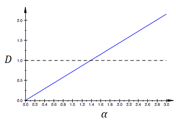
(a)(b)
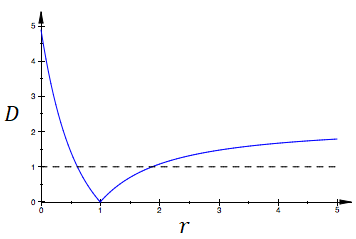
(c)

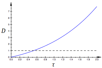
Figure 1: The blue curves represent the quantity $D$ from Theorem 4.1 plotted against the bifurcation parameters: $\alpha$ in (a) with $\tau=0.7$, $r=0.5$; $r$ in (b) with $\alpha=2.0$, $\tau=0.7$; and $\tau$ in (c) with $\alpha=2.0$, $r=0.5$. The intervals of $\alpha\in(0.0,1.4)$, $r\in(0.60,1.84)$, and $\tau\in(0.0,0.51)$ in which the blue curves are below the dashed horizontal line fulfill the sufficient condition of asymptotic stability of the equilibrium solution $v_{0}=\tau E$, following Theorem 4.1. Other parameters are fixed at $c=15.0$, $E=0.275$, $a_{e}=10.0$, $a_{i}=a_{e}/r$. The nonlinear dependence on $\tau$, as opposed to the linear dependence on $\alpha$, arises because in $\beta=\alpha c\tau F^{\prime}(v_{0})$, we get an additional dependence since $v_{0}=\tau E$.

We are interested in parameter constellations where spatiotemporal patterns emerge, that is, where the constant solution is not stable. From the diagrams, this requires that the memory decay $\alpha$ and the time constant $\tau$ of the synapses both be sufficiently large and the excitation and inhibition be sufficiently imbalanced. In fact, the case $r<1$, where inhibition is weaker, but more widely spread than excitation, is usually assumed in the literature to let $J$ acquire its Mexican hat shape. However, in this paper, we would use both cases: when $r<1$ (giving $J$ a Mexican-hat shape) and when $r>1$ (giving $J$ an inverse Mexican-hat shape.)

5 Dynamic bifurcations of the equilibrium solution

In Section 3, we have seen that static bifurcations are not possible since $\lambda=0$ is not a solution of (3.6). In this section, we investigate the conditions for oscillatory (dynamic) bifurcations. In case of a homogeneous neural field, we use the kernel function $J$ and the sigmoid transfer function $F$ in (2.4) and (2.5), respectively. Equation (3.6), which an infinitesimal perturbation $w(x,t)=e^{\lambda t}e^{ikx}$ needs to satisfy, can then be written as

$$\tau\lambda^{2}+(\tau\alpha+1)\lambda+\alpha =\alpha c\tau F^{\prime}(v_{0})\lambda\int_{-\infty}^{\infty}J(z)e^{-\lambda\frac{|z|}{\nu}}e^{-ikz}dz$$

$$=\beta\lambda\Bigg{[}\int_{-\infty}^{\infty}\Big{(}\frac{a_{e}}{2}e^{-|z|}-\frac{a_{i}r}{2}e^{-|z|r}\Big{)}e^{-\lambda\frac{|z|}{\nu}}e^{-ikz}dz\Bigg{]}$$

$$=\beta\lambda\Bigg{[}a_{e}\frac{1+\frac{\lambda}{\nu}}{(1+\frac{\lambda}{\nu})^{2}+k^{2}}-a_{i}r\frac{r+\frac{\lambda}{\nu}}{(r+\frac{\lambda}{\nu})^{2}+k^{2}}\Bigg{]}$$

$$-i\beta\lambda\Bigg{[}\frac{a_{e}k}{(1+\frac{\lambda}{\nu})^{2}+k^{2}}-\frac{a_{i}rk}{(r+\frac{\lambda}{\nu})^{2}+k^{2}}\Bigg{]}.$$ (5.1)

In (5) we shall consider the solution $\lambda$ as functions of $k$. The solution loses its stability when the real part of a root $\lambda$ in (5) changes from negative to positive. By tuning the parameters $r$, $\tau$ or $\alpha$, a critical point is eventually reached at $k=k_{c}$ in which the real part of the corresponding eigenvalue $\lambda(k_{c})$ of (5) become zero. From this critical point, one gets the critical wave-number $k_{c}$ and the critical frequency $\omega_{c}=\operatorname{Im}\lambda(k_{c})$. The case $k_{c}=0$ and $\omega_{c}\neq 0$ corresponds to a Hopf bifurcation folias2005breathers ; laing2005spiral ; folias2004breathing , and the case $k_{c}\neq 0$ and $\omega_{c}\neq 0$ to a Turing-Hopf bifurcation coombes2007modeling ; venkov2007dynamic ; touboul2012mean . We shall investigate both cases in more detail.

5.1 Hopf bifurcation

Now, we insert $\lambda=i\omega$ in (5), and because we are searching conditions for Hopf bifurcation (i.e., when $k_{c}=0$), we insert $k=k_{c}$ (so that the real part of the corresponding eigenvalue $\lambda|_{(k_{c}=0)}$ becomes zero) to get a polynomial of degree six in $\omega$ given by

$$q_{6}\omega^{6}+q_{5}\omega^{5}+q_{4}\omega^{4}+q_{3}\omega^{3}+q_{2}\omega^{2}+q_{1}\omega=0,$$ (5.2)

where the coefficients are given by

$$\begin{cases}\displaystyle{q_{6}=\frac{\tau}{\nu^{4}}},\\[5.69054pt] \displaystyle{q_{5}=\frac{\tau\alpha+1}{\nu^{4}}},\\[5.69054pt] \displaystyle{q_{4}=\frac{\tau(1+r^{2})}{\nu^{2}}+\frac{\beta(a_{e}-a_{i}r)}{\nu^{3}}-\frac{\alpha}{\nu^{4}}},\\[5.69054pt] \displaystyle{q_{3}=\frac{(r^{2}+1)(\tau\alpha+1)+\beta(a_{i}r-a_{e})}{\nu^{2}}},\\[5.69054pt] \displaystyle{q_{2}=\tau r^{2}+\frac{\beta r(a_{e}r-a_{i})}{\nu}-\frac{\alpha(1+r^{2})}{\nu^{2}}},\\[5.69054pt] \displaystyle{q_{1}=r^{2}(\tau\alpha+1)+\beta r(a_{i}-a_{e}r)}.\end{cases}$$ (5.3)

A trivial solution of (5.2) is $\omega=0$, but $\lambda$ should be purely imaginary, i.e., $\omega\neq 0$. However, this trivial solution allows us to reduce the degree of (5.2) to get

$$q_{6}\omega^{5}+q_{5}\omega^{4}+q_{4}\omega^{3}+q_{3}\omega^{2}+q_{2}\omega+q_{1}=0.$$ (5.4)

Substituting $\lambda=i\omega_{c}$ ($\omega_{c}\neq 0$) in (5.4) and separating the real and imaginary parts yields

$$\begin{cases}a_{3}\omega_{c}^{4}+a_{2}\omega_{c}^{2}+a_{1}=0,\\ b_{3}\omega_{c}^{4}+b_{2}\omega_{c}^{2}+b_{1}=0\end{cases}$$ (5.5)

where

$$\begin{cases}\displaystyle{a_{3}=\frac{1+\alpha\tau}{\nu^{4}},}\\[5.69054pt] \displaystyle{a_{2}=-\frac{\beta(a_{i}r-a_{e})+(\alpha\tau+1)(r^{2}+1)}{\nu^{2}},}\\[5.69054pt] \displaystyle{a_{1}=\beta r(a_{i}-a_{e}r)+r^{2}(\alpha\tau+1),}\\[5.69054pt] \displaystyle{b_{3}=\frac{\tau}{\nu^{4}},}\\[5.69054pt] \displaystyle{b_{2}={\frac{\alpha}{{\nu}^{4}}}-\frac{\beta(a_{e}-a_{i}r)}{\nu^{3}}-\frac{\tau(1+r^{2})}{\nu^{2}}},\\[5.69054pt] \displaystyle{b_{1}={r}^{2}\tau+\frac{\beta r(a_{e}r-a_{i})}{\nu}}-\frac{\alpha(1+r^{2})}{\nu^{2}}.\end{cases}$$ (5.6)

From the first equation of (5.5), we get

$$\omega_{c}^{2}={\frac{-a_{2}\pm\sqrt{{a_{2}}^{2}-4\,a_{1}\,a_{3}}}{2a_{3}}}.$$ (5.7)

Since $\omega_{c}\in\mathbb{R}-\{0\}$, $\omega_{c}^{2}>0$. And because $a_{3}>0$, (5.7) can be satisfied only if

$$\begin{cases}a_{i}r-a_{e}\geq 0,\\ \Gamma=\displaystyle{\big{[}\beta(a_{i}r-a_{e})+(\alpha\tau+1)(r^{2}+1)\big{]}^{2}-4\big{[}1+\alpha\tau\big{]}\big{[}\beta r(a_{i}-a_{e}r)+r^{2}(\alpha\tau+1)\big{]}\geq 0}.\end{cases}$$ (5.8)

When we substitute $\omega_{c}^{2}=({-a_{2}+\sqrt{{a_{2}}^{2}-4\,a_{1}\,a_{3}}})/2a_{3}$ into the second equation of (5.5), we obtain

$$\Big{[}\tau\,\Delta^{2}-\tau\,\left({r}^{2}+1\right)\Delta+{r}^{2}\tau\Big{]}\nu^{2}+\Big{[}\beta\,\left(a_{i}\,r-a_{e}\right)\Delta+\beta\,r\left(a_{e}\,r-a_{i}\right)\Big{]}\nu+\Big{[}\alpha\,\Delta-\alpha\,\left({r}^{2}+1\right)\Big{]}=0,$$ (5.9)

where

$$\Delta=\frac{1}{2\alpha\tau+2}\Bigg{[}\sqrt{-4\,\left(\alpha\,\tau+1\right)\left[\beta\,r\left(-a_{e}\,r+a_{i}\right)+\left(\alpha\,\tau+1\right){r}^{2}\right]+\left[\beta\,\left(a_{i}\,r-a_{e}\right)+\left(\alpha\,\tau+1\right)\left({r}^{2}+1\right)\right]^{2}}$$

$$\>\>\>\>+\beta\,\left(a_{i}\,r-a_{e}\right)+\left(\alpha\,\tau+1\right)\left({r}^{2}+1\right)\Bigg{]}.$$ (5.10)

The relations in (5.8) provide the parametric region in which the neural field oscillates due to Hopf bifurcation that occurs at $\omega_{c}^{2}=({-a_{2}+\sqrt{{a_{2}}^{2}-4\,a_{1}\,a_{3}}})/2a_{3}$ in (5.7) and which must also satisfy the first equation in (5.5). It is worth noting that in (5.8), the first condition is always satisfied (since in our analysis we always have $r=a_{e}/a_{i}$). Hence, it suffices to find the parametric regions where the second condition in (5.5) (i.e., $\Gamma\geq 0$) holds, for each parameter of interest. Fig.2(a) and (b) show the Hopf bifurcation curves for the parameters $\alpha$ and $\tau$, respectively. Fig.2 (c)-(e) show the Hopf bifurcation curves (in blue) in the parameter spaces $\alpha$-$\nu$, $\tau$-$\nu$, and $r$-$\nu$, respectively, in which the gray regions satisfy (5.8).

Fig. 3 shows corresponding space-time patterns of the membrane potential oscillating in different regions of the Hopf bifurcation parameter space of Fig.2(c). In Fig. 3(a)-(c), the values of the parameters $\nu$ and $\alpha$ are chosen below, on, and above the Hopf bifurcation curve of Fig.2(c), leading to different oscillatory regimes.

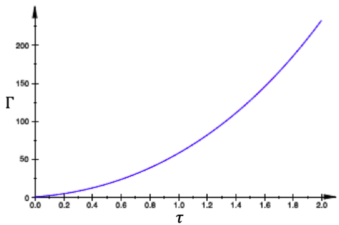
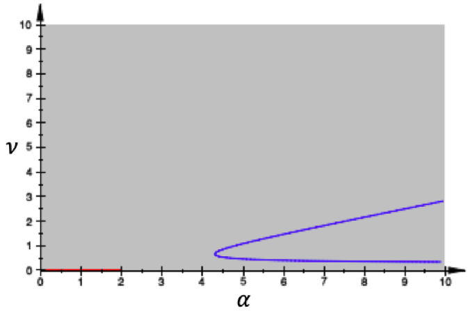
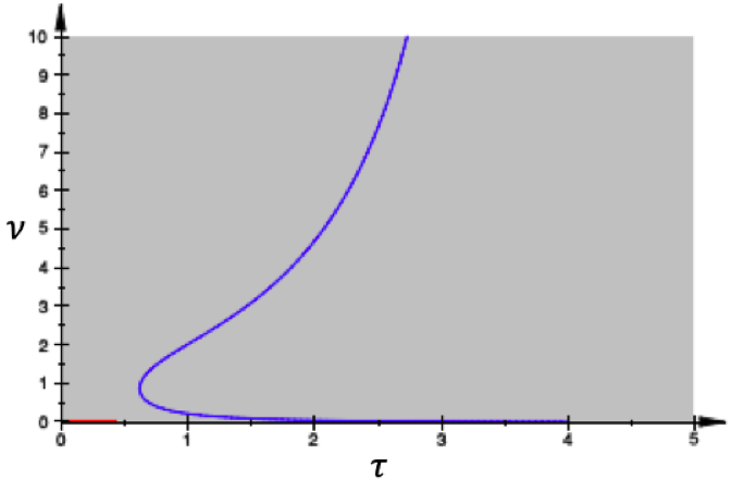
(a)(b) (c)(d) (e)

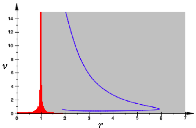
Figure 2: Panels (a) and (b) show the interval of $\alpha\in(0.0,8.0)$ and $\tau\in(0.0,2.0)$ for which (5.8) is satisfied. In the panels (c)-(e), the blue curves represent the solutions of (5.9) in the parameter spaces $\alpha$-$\nu$, $\tau$-$\nu$, and $r$-$\nu$, respectively. The gray areas in the panels represent the region of the parameter spaces where (5.8) holds, i.e., the oscillatory region. The parts of blue curves from (5.9) that lie in the gray region represent the values of the parameters for which oscillations exist, as these values satisfy (5.8). In (a) $\tau=0.75$, $r=5.0$; in (b) $\alpha=6.0$, $r=5.0$; in (c) $\tau=0.75$, $r=5.0$; in (d) $\alpha=6.0$, $r=5.0$; and in (e) $\alpha=6.0$, $\tau=0.75$. In (a)-(e), the other parameter values are: $c=15.0$, $E=0.275$, $a_{e}=10.0$, $v_{0}=\tau E$, $\beta=\alpha c\tau F^{\prime}(v_{0})$, and in (e) $a_{i}=a_{e}/r$.

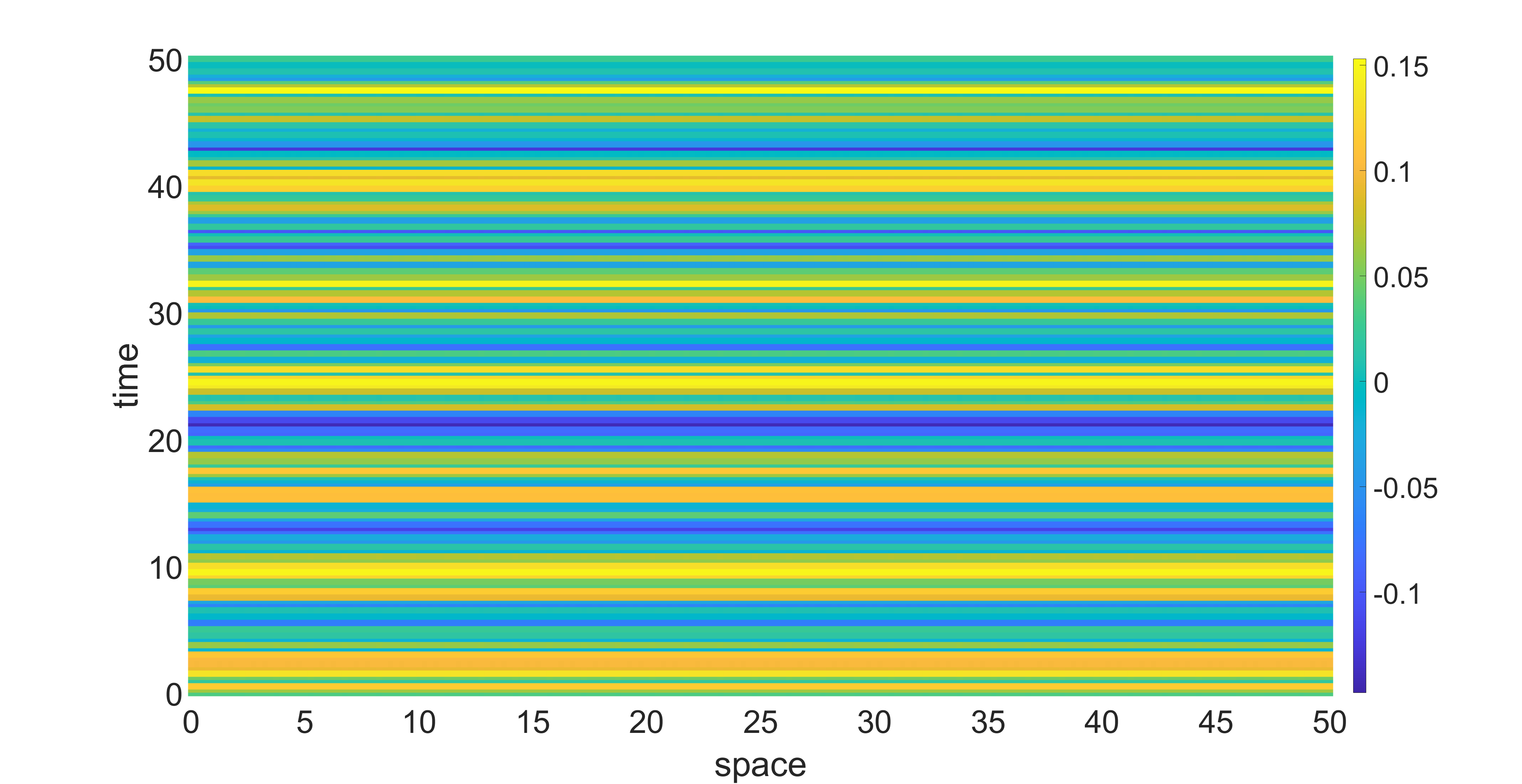
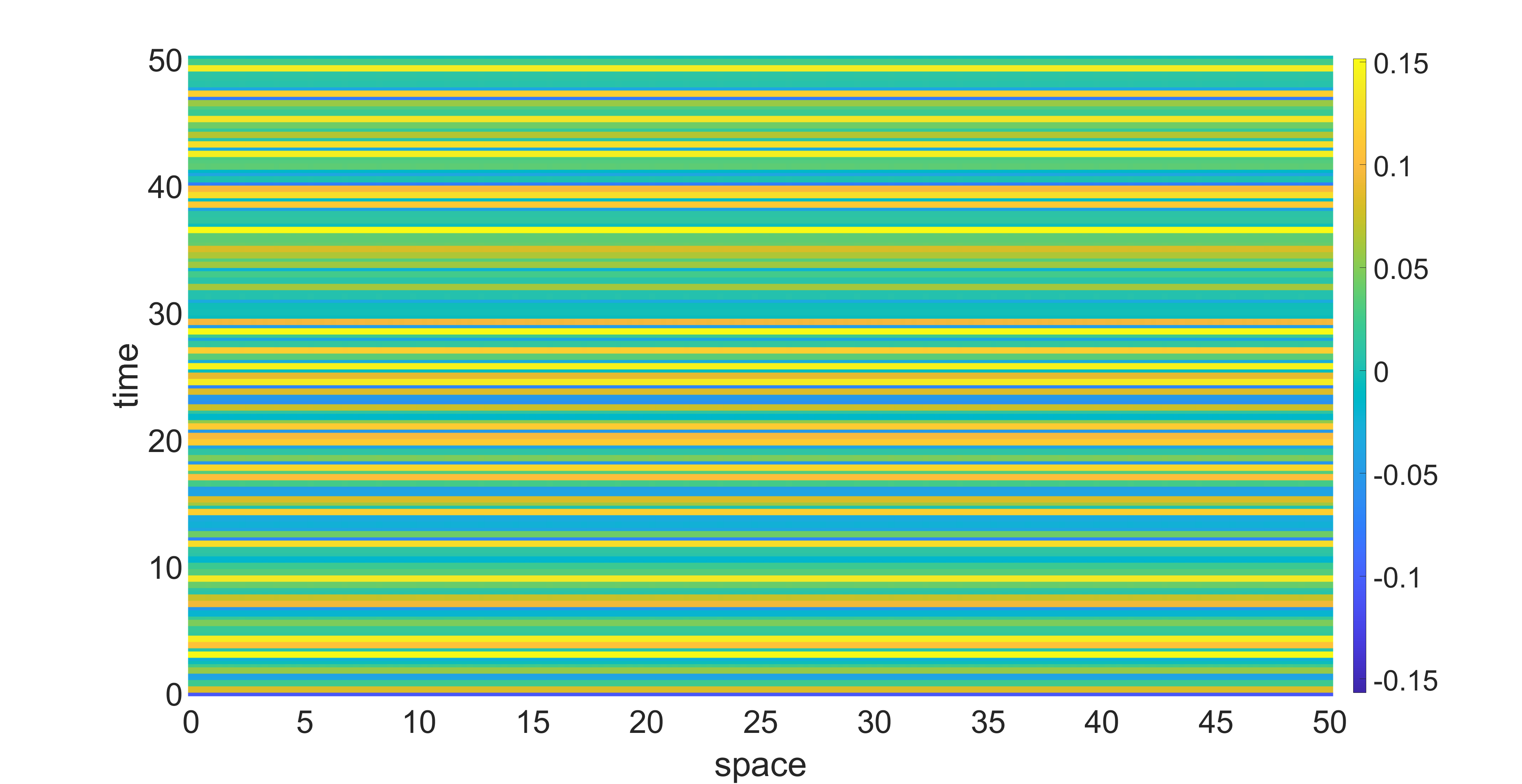
(a)(b) (c)

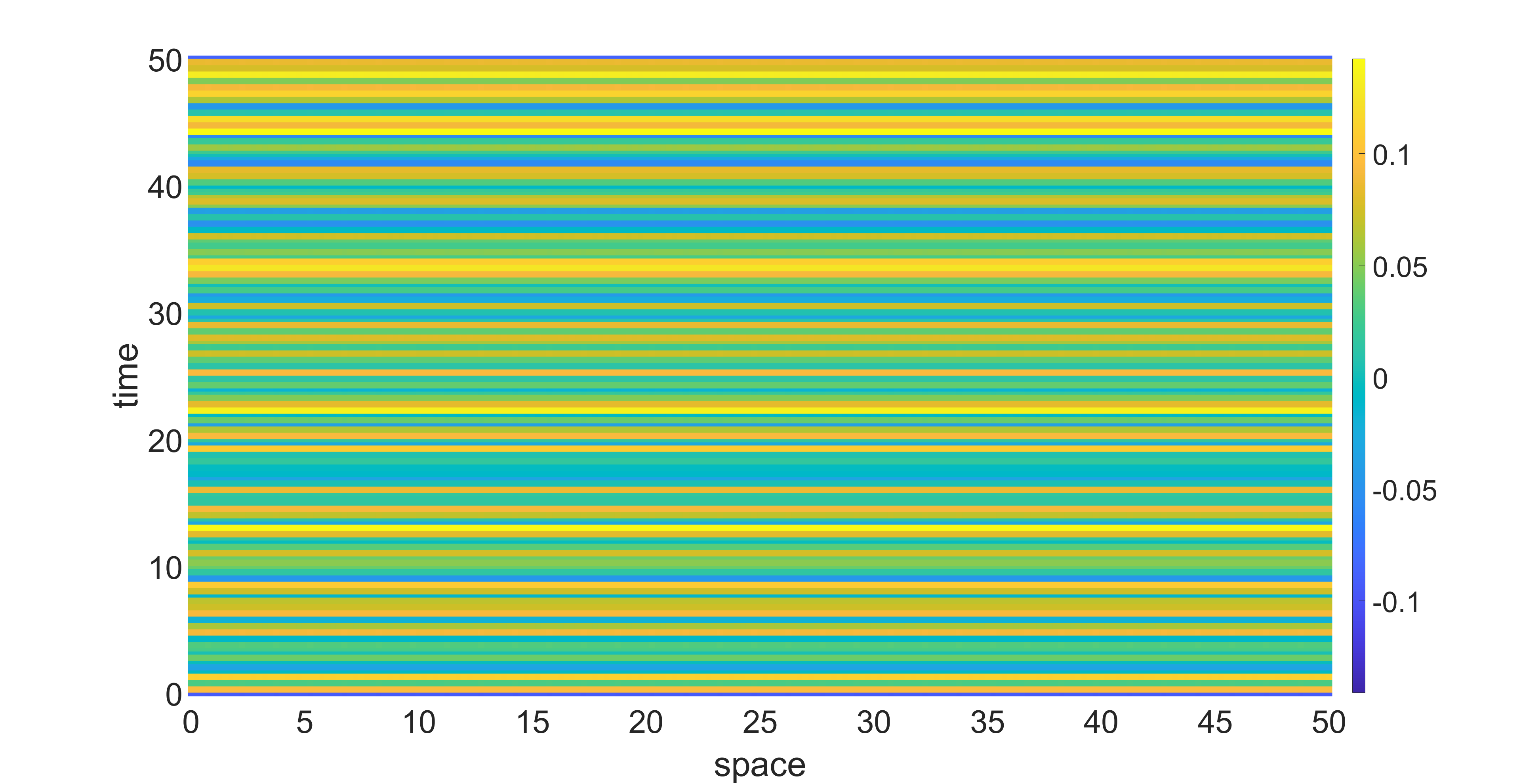
Figure 3: Panels (a)–(c) show color coded space-time patterns of the membrane potential $v(x,t)$ emerging from Hopf instability. In (a), $\alpha=7.0$, $\nu=0.16$, i.e., below the Hopf bifurcation (blue) curve. In (b), $\alpha=7.0$, $\nu=1.83$, i.e., on the Hopf bifurcation curve. In (c), $\alpha=7.0$, $\nu=2.5$, i.e., above the Hopf bifurcation curve. In all cases, we have periodic oscillations of spatially constant solutions. In the panels, the solutions are obtained for the Gaussian connectivity kernel, with initial conditions chosen randomly from a uniform distribution on $[v_{0}-0.1,v_{0}+0.1]$. Other parameters are fixed at $\tau=0.75$, $a_{e}=10.0$, $a_{i}=2.0$, $r=a_{e}/a_{i}=5.0$, $c=15.0$, and $k=0$.

5.2 Turing-Hopf bifurcation

Theorem 5.1

Let $D$ be defined as in Theorem (4.1). Then there exists $B>0$ depending only on $L$ and $D$ such that

$$|\omega|\leq B$$ (5.11)

whenever $w(x,t)=e^{i\omega t}e^{ikx}$, $\omega,k\in\mathbb{R}$, is a solution of (3). Furthermore, if $D<1$, then there exists $A>0$, depending on $L$ and $D$, such that

$$0<A\leq|\omega|.$$ (5.12)

In particular, if $L(\lambda)=\tau\lambda+1$, then

$$\tau^{2}\omega^{2}\leq D^{2}-1.$$ (5.13)

Proof

If $\lambda=i\omega$ satisfies the dispersion relation (3.6) for some $k$, then

$$|L(i\omega)|\leq\beta\int_{-\infty}^{\infty}|J(z)|dz=D.$$ (5.14)

Since $|L(i\omega)|\rightarrow\infty$ as $\omega\rightarrow\pm\infty$ for any non-constant polynomial $L$, the above inequality implies an upper bound $B$ on $|\omega|$, which proves (5.11). For the particular case $L(\lambda)=\tau\lambda+1$, (5.14) gives

$$|L(i\omega)|^{2}=\tau^{2}\omega^{2}+1\leq D^{2},$$ (5.15)

which proves (5.13).

The following analytical result will be used in the rest of the numerical computations. The conditions for Turing-Hopf bifurcation require that with the Fourier-Laplace ansatz (3.3), that is, $w(x,t)=e^{\lambda t}e^{ikx}$, we find $\lambda=\pm i\omega$ with $\omega\neq 0$ at some critical value $k_{c}\neq 0$. Inserting $\lambda=i\omega$ in (3.6), we obtain

$$L(i\omega):=1+i\tau\omega=\beta\Big{(}\frac{i\omega}{\alpha+i\omega}\Big{)}\int_{-\infty}^{\infty}J(z)e^{-i\omega\frac{|z|}{\nu}}e^{ikz}dz,$$ (5.16)

which yields upon expansion,

$$\beta\frac{\omega^{2}+i\alpha\omega}{\alpha^{2}+\omega^{2}}\int_{-\infty}^{\infty}J(z)e^{-\frac{i\omega\left|z\right|}{\nu}}\cos(kz)dz =\beta\frac{\omega^{2}+i\alpha\omega}{\alpha^{2}+\omega^{2}}\int_{-\infty}^{\infty}J(z)\Big{[}\cos\Big{(}\frac{\omega\left|z\right|}{\nu}\Big{)}-i\sin\Big{(}\frac{\omega\left|z\right|}{\nu}\Big{)}\Big{]}\cos(kz)dz$$

$$=\frac{\beta}{2}\frac{\omega^{2}+i\alpha\omega}{\alpha^{2}+\omega^{2}}\int_{-\infty}^{\infty}J(z)\left[e^{i\left|z\right|(\frac{\omega}{\nu}+k)}+e^{i\left|z\right|(\frac{\omega}{\nu}-k)}\right]dz.$$ (5.17)

By substituting the power series

$$e^{i\left|z\right|(\frac{\omega}{\nu}\pm k)}=\sum_{m=0}^{N}\frac{i^{m}(\frac{\omega}{\nu}\pm k)^{m}}{m!}\left|z\right|^{m}+O(\nu^{-(N+1)}),$$

(5.2) is written as

$$\frac{\beta}{2}\frac{\omega^{2}+i\alpha\omega}{\alpha^{2}+\omega^{2}}\int_{-\infty}^{\infty}J(z)\Big{(}\sum_{m=0}^{N}\frac{i^{m}}{m!}\left[\Big{(}\frac{\omega}{\nu}+k\Big{)}^{m}+\Big{(}\frac{\omega}{\nu}-k\Big{)}^{m}\right]\left|z\right|^{m}+O(\nu^{-(N+1)})\Big{)}dz.$$ (5.18)

We define $J_{m}$ as

$$J_{m}:=\int_{-\infty}^{\infty}J(z)\left|z\right|^{m}dz$$ (5.19)

and the integrals are assumed to exist. Substituting (5.19) into (5.18) yields

$$L(i\omega)=\beta\frac{\omega^{2}+i\alpha\omega}{\alpha^{2}+\omega^{2}}\left[J_{0}+i\frac{\omega}{\nu}J_{1}-\frac{1}{2!}\Big{(}k^{2}+\frac{\omega^{2}}{\nu^{2}}\Big{)}J_{2}+\cdots\right].$$ (5.20)

Equating the right-hand side of (5.20) to the left-hand side of (5.16), we get

$$1+i\tau\omega=\beta\frac{\omega^{2}+i\alpha\omega}{\alpha^{2}+\omega^{2}}\left[J_{0}+i\frac{\omega}{\nu}J_{1}-\frac{1}{2!}\Big{(}k^{2}+\frac{\omega^{2}}{\nu^{2}}\Big{)}J_{2}+\cdots\right].$$ (5.21)

The number of terms required for the above series to be helpful depends on the values of $\nu$ and $k$ as well as the shape of the kernel $J$. If $J$ is highly concentrated near the origin, as in our case (see (2.4)) or, more generally, if $J$ is of exponential order, then a few terms will suffice. That is, assume there exist positive numbers $\kappa_{1}$ and $\kappa_{2}$ such that

$$\left|J(z)\right|\leq\kappa_{1}e^{-\kappa_{2}\left|z\right|}\quad\text{ for all $z\in\mathbb{R}$}.$$ (5.22)

Then by (5.19)

$$\left|J_{m}\right|\leq\int_{-\infty}^{\infty}\left|z\right|^{m}\kappa_{1}e^{-\kappa_{2}\left|z\right|}dz=2\kappa_{1}\int_{0}^{\infty}z^{m}e^{-\kappa_{2}z}dz=2\kappa_{1}\kappa_{2}^{-(m+1)}\Gamma(m+1)=2\kappa_{1}\kappa_{2}^{-(m+1)}m!$$

so the $m$th term in the series (5.21) is bounded in absolute value by

$$2\frac{\kappa_{1}}{\kappa_{2}}\Big{(}\frac{\left|\omega\right|}{\kappa_{2}\nu}\Big{)}^{m}\leq 2\frac{\kappa_{1}}{\kappa_{2}}\Big{(}\frac{B}{\kappa_{2}\nu}\Big{)}^{m},$$

where we have used Theorem 5.1 to bound the values of $\omega$. In the case of a high transmission speed $\nu$ or $B$ (for example small $\beta$) or a large value of $\kappa_{2}$ (rapid decrease of $J$ away from the origin) or a bounded value of $k$, the finite series has increased precision. At least one of these conditions is assumed to be true, so a small number of terms are sufficient to determine the general behavior. In order to observe the qualitative effects of a finite transmission speed, we therefore neglect the terms from the fourth and higher orders in the series (5.21).

Equating the real parts of both sides in (5.21), and similarly with the imaginary parts, and considering $\omega\neq 0$ (a Turing-Hopf bifurcation condition), we have

$$\begin{cases}\begin{split}1=\frac{\beta}{\alpha^{2}+\omega^{2}}\left[\omega^{2}J_{0}-\alpha\omega\left(\frac{\omega}{\nu}J_{1}\right)-\omega^{2}\frac{1}{2!}(k^{2}+\frac{\omega^{2}}{\nu^{2}})J_{2}\right],\\[7.11317pt] \tau=\frac{\beta}{\alpha^{2}+\omega^{2}}\left[\alpha J_{0}+\omega\left(\frac{\omega}{\nu}J_{1}\right)-\frac{1}{2!}\alpha\Big{(}\big{(}k^{2}+\frac{\omega^{2}}{\nu^{2}}\big{)}J_{2}\Big{)}\right].\end{split}\end{cases}$$ (5.23)

From (5.23) we have

$$\frac{\tau}{\alpha J_{0}+\frac{\omega^{2}}{\nu}J_{1}-\frac{\alpha}{2}\Big{(}k^{2}+\frac{\omega^{2}}{\nu^{2}}\Big{)}J_{2}}=\frac{\beta}{\alpha^{2}+\omega^{2}}=\frac{1}{\omega^{2}J_{0}-\alpha\frac{\omega^{2}}{\nu}J_{1}-\frac{\omega^{2}}{2}\Big{(}k^{2}+\frac{\omega^{2}}{\nu^{2}}\Big{)}J_{2}},$$ (5.24)

which gives

$$\alpha J_{0}+\frac{\omega^{2}}{\nu}J_{1}-\frac{\alpha}{2}\Big{(}k^{2}+\frac{\omega^{2}}{\nu^{2}}\Big{)}J_{2}=\tau\omega^{2}J_{0}-\tau\alpha\frac{\omega^{2}}{\nu}J_{1}-\tau\frac{\omega^{2}}{2}\Big{(}k^{2}+\frac{\omega^{2}}{\nu^{2}}\Big{)}J_{2}.$$ (5.25)

After substituting (2.4) into (5.19), the convergent improper integrals $J_{n}$ $(n=0,1,2)$ are explicitly calculated as

$$\begin{split}&J_{0}=-a_{i}+a_{e},\\[2.84526pt] &J_{1}=\frac{ra_{e}-a_{i}}{r},\\[2.84526pt] &J_{2}=\frac{2(r^{2}a_{e}-a_{i})}{r^{2}}.\end{split}$$ (5.26)

Substituting (5.26) into (5.25), we obtain

$$\frac{\tau}{\nu^{2}}\Bigg{(}\frac{r^{2}a_{e}-a_{i}}{r^{2}}\Bigg{)}\omega^{4}+\Bigg{[}\tau(a_{i}-a_{e})+\Big{(}\tau k^{2}-\frac{\alpha}{\nu^{2}}\Big{)}\Big{(}\frac{r^{2}a_{e}-a_{i}}{r^{2}}\Big{)}+\Big{(}\frac{\alpha\tau+1}{\nu}\Big{)}\Big{(}\frac{ra_{e}-a_{i}}{r}\Big{)}\Bigg{]}\omega^{2}$$

$$+\alpha\Bigg{(}(a_{e}-a_{i})-k^{2}\Big{(}\frac{r^{2}a_{e}-a_{i}}{r^{2}}\Big{)}\Bigg{)}=0.$$ (5.27)

Thus, (5.2) represents the Turing-Hopf bifurcation in the parameter space ($\alpha,\nu,\tau,r,a_{e},a_{i}$) for some $k\neq$ and $\omega\neq 0$. We use (5.2) to obtain the results presented in Figs.4, 5, and 7.

In Fig.4, we show a dispersion relation (i.e., a $k$–$\omega$ curve) of the neural field for a particular set of values of the other parameters, i.e., $\alpha=5.0,\nu=1.0,\tau=0.75,r=5.0,a_{e}=10.0,$ and $a_{i}=a_{e}/r=2.0$.

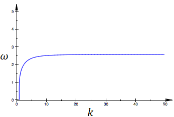
Figure 4: A dispersion relation of the neural field satisfying the Turing-Hopf bifurcation equation given by (5.2) for a fixed set of parameters values: $\alpha=5.0$, $\nu=1.0$, $\tau=0.75$, $r=5.0$, $a_{e}=10.0$, $a_{i}=a_{e}/r=2.0$.

In Fig.5(a)–(d), we respectively show the Turing-Hopf bifurcation curves in different parameter spaces: ($\alpha$-$\omega$), ($\nu$-$\omega$), ($\tau$-$\omega$), and ($r$-$\omega$) for a fixed value of the spatial mode $k=25.0$. We note from Fig.5(a) and (c) that the memory decay $\alpha$ and the leakage parameter $\tau$ have opposite effects. The former increases the frequency $\omega$ of the oscillations, whereas the latter decreases it. From Fig.5(b), the transmission speed $\nu$ has a nonmonotonic influence, with a minimum for $\omega$ at a particular value of $\nu$. Similarly, Fig.5(d), the ratio of the excitatory and inhibitory synaptic weights $r$ has a nonmonotonic influence on $\omega$. However, when the excitatory and inhibitory synaptic weights are balanced, i.e., when $r=a_{e}/a_{i}=1$, (5.2) has many trivial solutions, that is, there exist infinitely many $\omega$ values that satisfy (5.2). This explains the vertical line in Fig.5(d) and Fig.7(d) at $r=1$.

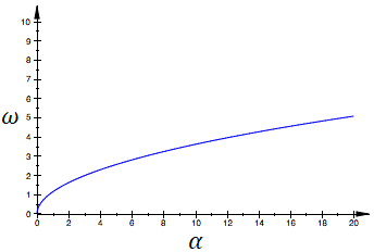
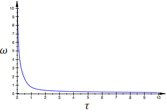
(a)(b)
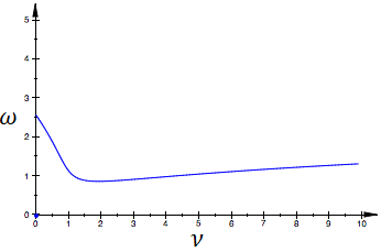
(c)(d)

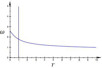
Figure 5: The curves in panels (a)-(d) represent the Turing Hopf bifurcation curves in (5.2) in the ($\alpha$-$\omega$), ($\nu$-$\omega$), ($\tau$-$\omega$), and ($r$-$\omega$) planes, respectively. Parameter values are: (a) $k=25.0$, $\nu=1.0$, $\tau=0.75$, $r=5.0$; (b) $k=1.0$, $\alpha=5.0$, $\tau=0.75$, $r=5.0$; (c) $k=1.0$, $\alpha=5.0$, $\nu=1.0$, $r=5.0$; (d) $k=1.0$, $\alpha=5.0$, $\nu=1.0$, $\tau=0.75$. The remaining parameters are fixed at $a_{e}=10.0$, $a_{i}=a_{e}/r$.

In Fig.6, we display the space-time patterns in three distinct regions of the Turing-Hopf bifurcation curve of Fig.5(a), for example. Here, one can see, as expected, that the Turing-Hopf bifurcation leads to spatially and temporally non-constant solutions. With values fixed at $k=25.0$, $\nu=1.0$, $\tau=0.75$, $r=5.0$ $a_{e}=10.0$, and $a_{i}=a_{e}/r=2.0$, we chose a value for the exponential temporal kernel $\alpha$ and then calculate the corresponding temporal mode $\omega$ from (5.2), such that both values ($\alpha,\omega$) lie above (as in Fig.6(a)), on (as in Fig.6(b)), and below (as in Fig.6(c)) the Turing-Hopf bifurcation curve in Fig.5(a). Comparing the patterns in Fig.6(a), (b), and (c), one can clearly see that for a total time interval of 10 units, there is a change in the number of temporal oscillations, while the number of spatial oscillations does not change (because, of course, the spatial mode is fixed at $k=25.0$). In Fig.6(a), with the values of $\omega$ and $\alpha$ lying above the Turing-Hopf bifurcation curve, the neural field admits temporal oscillations with a relatively high frequency (12 oscillations per 10 units time, i.e., $1.2$ hertz (Hz)). In Fig.6(b) with $\omega$ and $\alpha$ lying on the Turing-Hopf bifurcation curve, the frequency is reduced to 0.6 Hz, and in Fig.6(c), with $\omega$ and $\alpha$ lying below the Turing-Hopf bifurcation curve, the frequency is further reduced to 0.2 Hz.

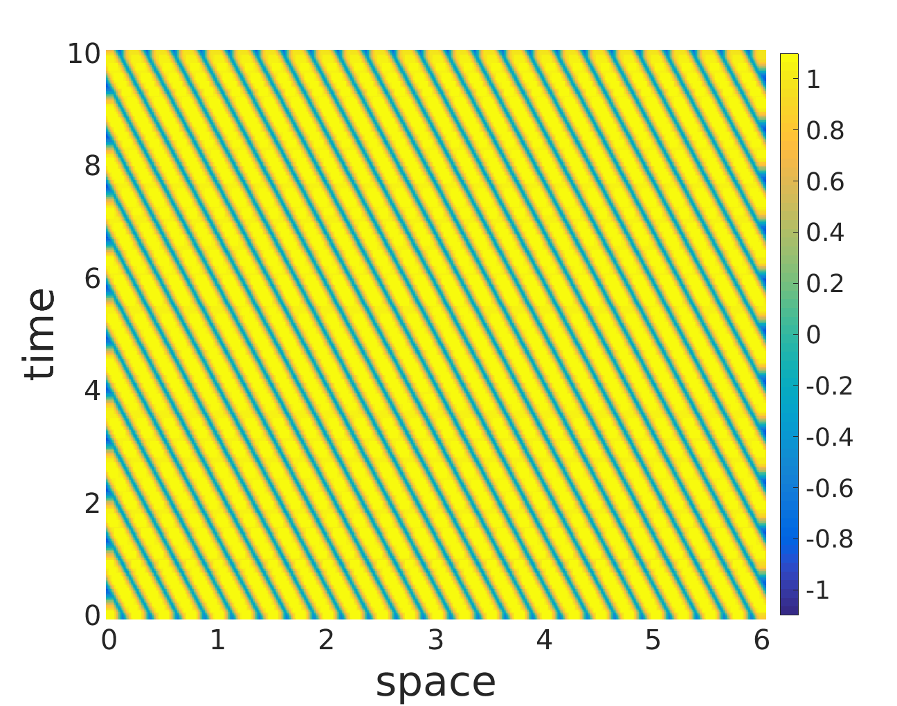
(a) (b)
(c)

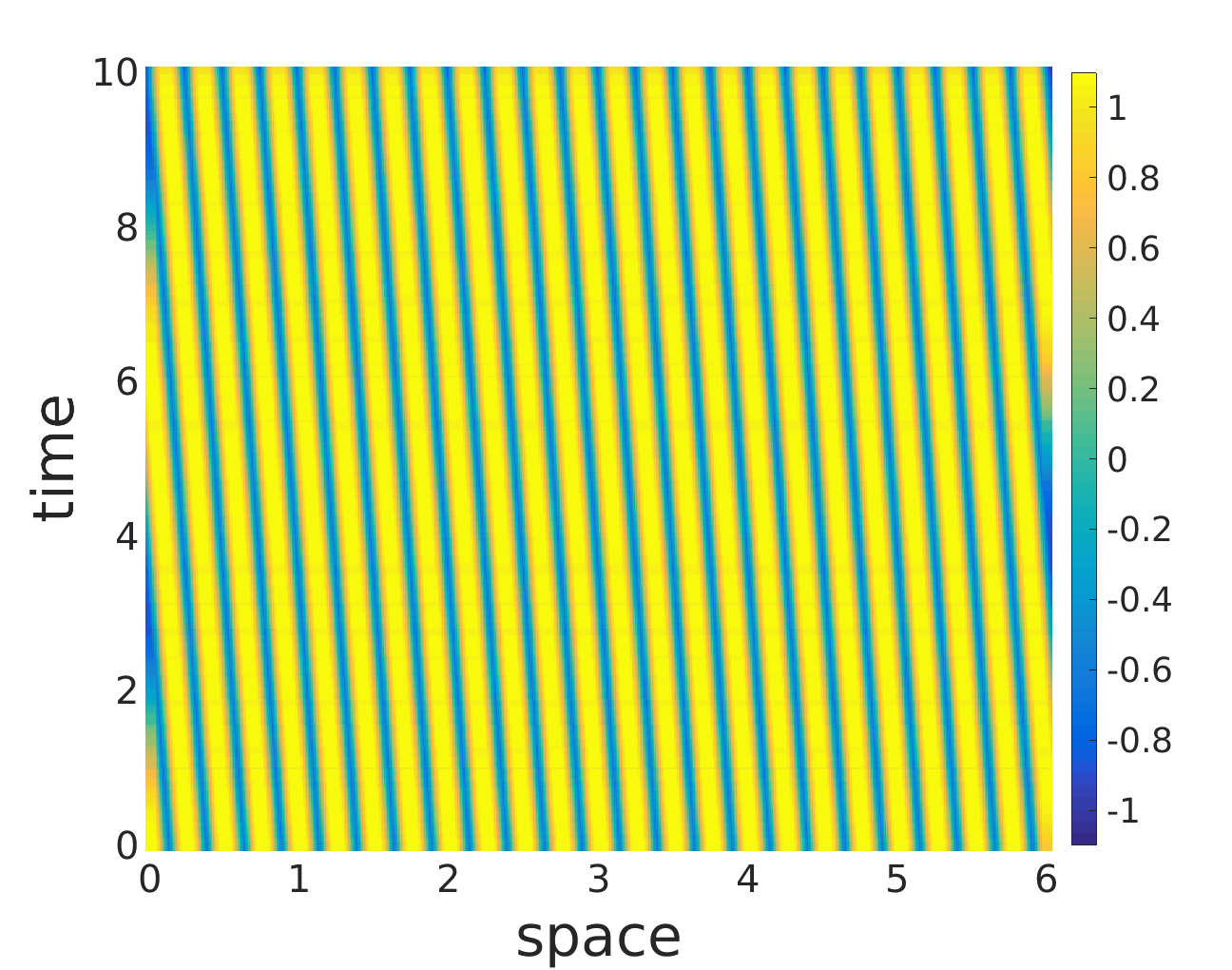
Figure 6: Panels (a)-(c) show color coded space-time patterns of the membrane potential $v(x,t)$ emerging from a Turing-Hopf instability, leading to periodic oscillations of spatially and temporally non-constant solutions, obtained with the Gaussian connectivity kernel. Initial conditions are chosen randomly from a uniform distribution on $[v_{0}-0.1,v_{0}+0.1]$. In panel (a), $(\alpha,\omega)=(10.0,1.0)$ lies above the Turing-Hopf bifurcation curve of Fig.5(a). In (b), $(\alpha,\omega)=(10.0,3.62)$ lies on this Turing-Hopf bifurcation curve, and in (c) $(\alpha,\omega)=(10.0,7.0)$ lies below the curve. We observe a decrease in the frequency of the temporal oscillations of Turing-Hopf patterns from panel (a) to (c), and a constant frequency in the spatial oscillations. Parameter values are: $a_{e}=10.0$, $r=5.0$, $a_{i}=a_{e}/r=2.0$, $\nu=1.0$, $\tau=0.75$, $k=25.0$.

In Fig.7(a)-(d), we show the Turing-Hopf bifurcation curves in different parameter spaces: ($\alpha$-$k$), ($\nu$-$k$), ($\tau$-$k$), and ($r$-$k$), respectively, for a fixed value of the temporal mode $\omega=0.1$. We should contrast these relations with those of Fig. 5. In effect, the dependence of the temporal and of the spatial frequency values at the bifurcation on those other parameters is essentially opposite.

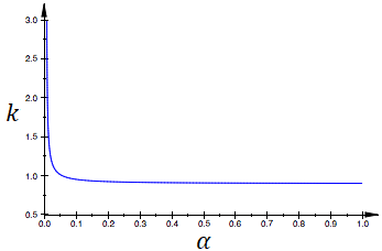
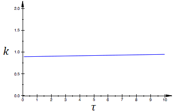
(a)(b)
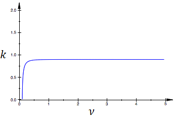
(c)(d)

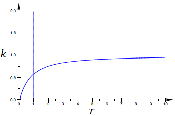
Figure 7: The curves in panels (a)-(d) represent the Turing Hopf bifurcation curves in (5.2) in the ($\alpha$-$k$), ($\nu$-$k$), ($\tau$-$k$), and ($r$-$k$) planes, respectively. Parameter values are: (a) $\omega=0.1$, $\nu=1.0$, $\tau=0.75$, $r=5.0$; (b) $\omega=0.1$, $\alpha=5.0$, $\tau=0.75$, $r=5.0$; (c) $\omega=0.1$, $\alpha=5.0$, $\nu=1.0$, $r=5.0$; (d) $\omega=0.1$, $\alpha=5.0$, $\nu=1.0$, $\tau=0.75$. The remaining parameters are fixed at $a_{e}=10.0$, $a_{i}=a_{e}/r$.

In Fig.8, we display the space-time patterns in three distinct regions of the Turing-Hopf bifurcation curve of Fig.7(a), for example. One can also see, that the Turing-Hopf bifurcation leads to spatially and temporally non-constant solutions. Here, for the sake of comparison, we have also fixed the parameters to the same values given in Fig.6, i.e., $\nu=1.0$, $\tau=0.75$, $r=5.0$ $a_{e}=10.0$, $a_{i}=a_{e}/r=2.0$, and temporal mode parameter is fixed at $\omega=0.1$. As in Fig.6, the patterns in Fig.8 are obtained with values of the spatial frequency $k$ and the exponential temporal kernel $\alpha$, where we choose $\alpha$ and then calculate the corresponding spatial frequency $k$ from (5.2), such that both values ($\alpha,k$) lie above (as in Fig.8(a)), on (as in Fig.8(b)), and below (as in Fig.8(c)) the Turing-Hopf bifurcation curve in Fig.7(a).

Comparing the panels in Fig.8, one can see a change in the patterns already observed in Fig.6, but in terms of the frequency of the spatial oscillations, for a total space interval of 50 units and a temporal mode fixed at $\omega=0.1$. In Fig.8(a), $k$ and $\alpha$ which are above the Turing-Hopf bifurcation curve in Fig.7(a), and the neural field oscillates with a relatively high spatial frequency i.e., 0.26 Hz. In Fig.8(b), $k$ and $\alpha$ lie on the Turing-Hopf bifurcation curve, and the spatial frequency of oscillation is reduced 0.16 Hz. And in Fig.8(c), $k$ and $\alpha$ lie below the Turing-Hopf bifurcation curve, and spatial frequency is further reduced to 0.1 Hz. However, in terms of the wavelengths in both space and time, the space-time patterns of the Turing-Hopf bifurcation in Fig.6 and Fig.8 are different: Fig.8 shows fewer oscillations on larger space and longer time intervals than in Fig.6.

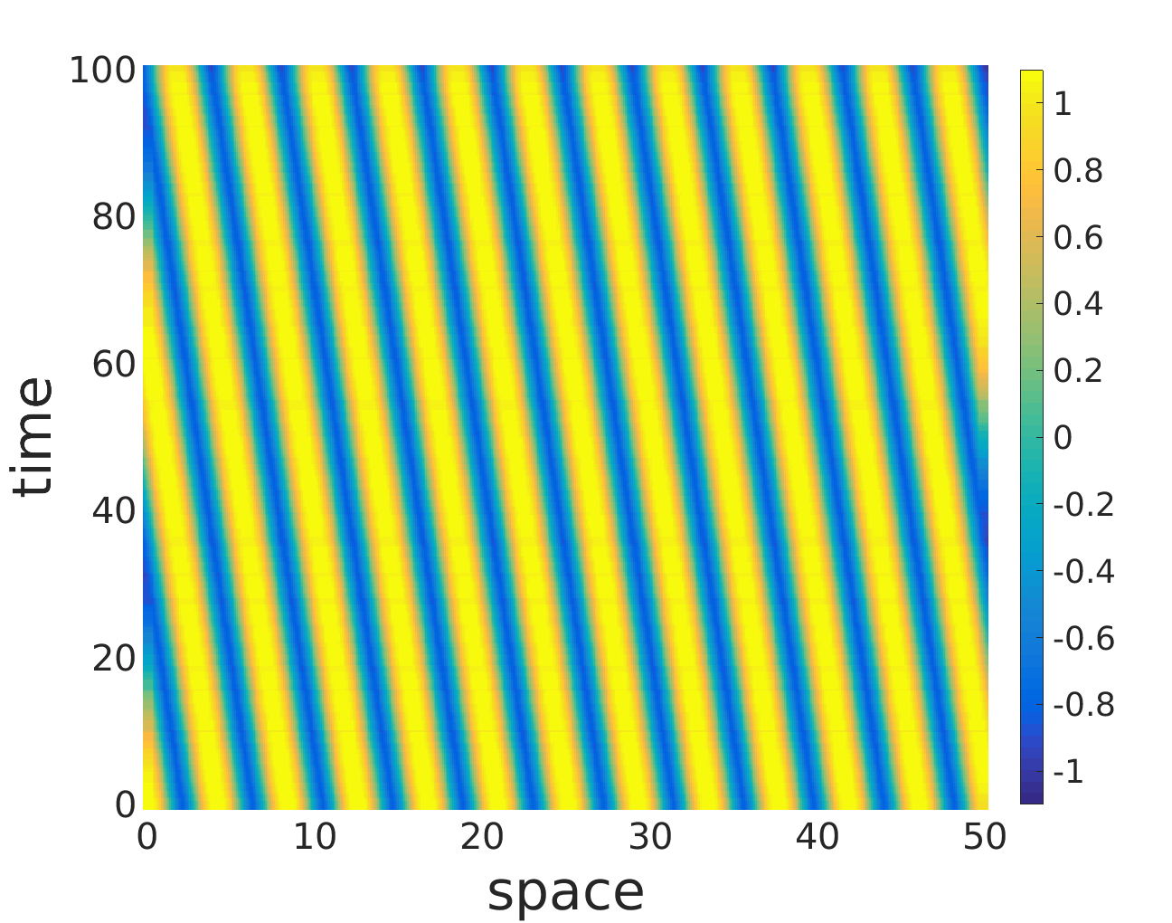
(a)(b)
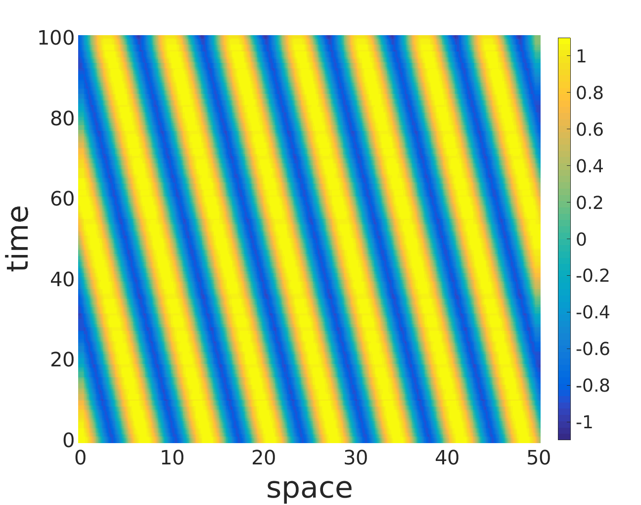
(c)

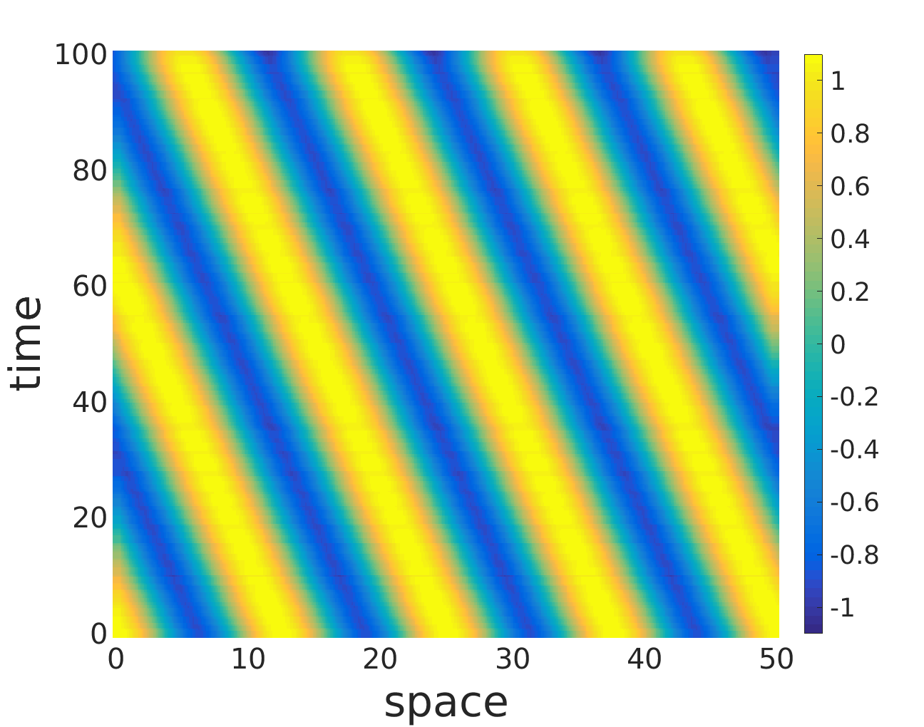
Figure 8: Panels (a)-(c) show color coded space-time patterns of membrane potential $v(x,t)$ emerging from Turing-Hopf instability. leading to periodic oscillations of spatially and temporally non-constant solutions, obtained with the Gaussian connectivity kernel. Initial conditions are chosen randomly from a uniform distribution on $[v_{0}-0.1,v_{0}+0.1]$. In panel (a), $(\alpha,k)=(0.5,0.5)$ lies above the Turing-Hopf bifurcation curve of Fig.7(a). In (b), $(\alpha,k)=(0.5,0.907)$ lies on this Turing-Hopf bifurcation curve, and $(\alpha,k)=(0.5,1.5)$ lies below this curve. We observe a decrease in the frequency of the spatial oscillations of Turing-Hopf patterns from panel (a) to (c), and a constant frequency in the temporal oscillations. Parameter values are: $a_{e}=10.0$, $r=5.0$, $a_{i}=a_{e}/r=2.0$, $\nu=1.0$, $\tau=0.75$, $\omega=0.1$.

6 Concluding remarks

In this paper we have studied the bifurcation behavior and the wave patterns generated by a neural field equation with an exponential temporal kernel. The exponential temporal kernel in (2.2) takes into account the finite memory of past activities of the neurons, which the Green’s function utilized in atay2004stability does not.

Our first observation was that static bifurcations such as saddle-node and pitchfork, as well as static Turing patterns, are not possible with an exponential temporal kernel, because the characteristic polynomial does not have an eigenvalue 0. This is in contrast to atay2004stability , where the temporal kernel was taken as the Green’s function rather than an exponential function, and thus allowed zero eigenvalues.

The dynamic bifurcations, however, turn out to be interesting. In the analysis of the dynamic bifurcations of the equilibrium solution, we have obtained the conditions for the occurrence of Hopf and Turing-Hopf bifurcations. Furthermore, we have numerically illustrated these dynamic bifurcations with bifurcation diagrams and space-time patterns.

On one hand, this shows that neural fields can generate rich spatio-temporal patterns. In our analysis, we needed transmission delays and exponentially decaying memory, both of which make sense from a neurophysiological perspective. On the other hand, these findings support, at least in qualitative terms, neurophysiological models of cognition, like those of malsburg1981 ; abeles1982 and many subsequent ones, that depend on such spatio-temporal patterns.

Declarations

Conflict of interest All authors declare that they have no known competing financial interests or personal relationships that could have appeared to influence the work reported in this paper.

Authors’ contributions ES and MEY performed the theoretical analysis and numerical simulations, analyzed the results, and wrote the manuscript. FMA analyzed the results and wrote the manuscript. JJ designed the study, analyzed the results, and wrote the manuscript. All authors reviewed the manuscript.

References

- (1) J.Y.Wu, X.Y. Huang, C. Zhang. Propagating waves of activity in the neocortex: what they are, what they do. Neuroscientist. 2008 Oct;14(5):487-502. doi: 10.1177/1073858408317066. PMID: 18997124; PMCID: PMC2679998.
- (2) Townsend, R.G., Solomon, S.S., Chen, S.C., Pietersen, A.N., Martin, P.R., Solomon, S.G. and Gong, P., 2015. Emergence of complex wave patterns in primate cerebral cortex. Journal of Neuroscience, 35(11), pp.4657-4662.
- (3) Lubenov, E., Siapas, A. Hippocampal theta oscillations are traveling waves. Nature 459, 534–539 (2009). https://doi.org/10.1038/nature08010
- (4) von der Malsburg, C. (1981). The correlation theory of brain function. Internal report 81-2, MPI biophysical chemistry. Reprinted in E. Domany, J. L. van Hemmen, & K. Schulten (Eds.), Models of neural networks II, chap. 2 (pp. 95–119). Berlin: Springer (1994).
- (5) Abeles, M. (1982). Studies of brain function: Vol. 6. Local cortical circuits: An electro-physiological study. Berlin: Springer.
- (6) Galinsky VL, Frank LR. Brain Waves: Emergence of Localized, Persistent, Weakly Evanescent Cortical Loops. J Cogn Neurosci. 2020 Nov;32(11):2178-2202. doi: 10.1162/jocn-a-01611. Epub 2020 Jul 21. PMID: 32692294; PMCID: PMC7541648.
- (7) E.R. Kandel, J.H. Schwartz, T.M. Jessell, Department of Biochemistry, Molecular Biophysics Thomas Jessell, S. Siegelbaum, A.J. Hudspeth, Principles of neural science, vol 4, McGraw-hill, New York, 2000.
- (8) H.R. Wilson, J.D. Cowan, A mathematical theory of the functional dynamics of cortical and thalamic nervous tissue, Biol. Cybernet. 13 (1973) 55-80.
- (9) H.R. Wilson, J.D. Cowan, Excitatory and inhibitory interactions in localized populations of model neurons, Biophys. J. 12 (1972) 1-24.
- (10) S.-I. Amari, Dynamics of pattern formation in lateral-inhibition type neural fields, Biol. Cybernet. 27 (1977) 77-87.
- (11) R. Veltz, O. Faugeras, Stability of the stationary solutions of neural field equations with propagation delays, J. Math. Neurosci. 1 (2011) 1.
- (12) L.I. Perlovsky, Toward physics of the mind: Concepts, emotions, consciousness, and symbols, Phys. Life Rev. 3 (2006) 23–55.
- (13) J. Alswaihli, R. Potthast, I. Bojak, D. Saddy, A. Hutt, Kernel reconstruction for delayed neural field equations, J. Math. Neurosci. 8 (2018) 3.
- (14) A.H. Abbassian, M. Fotouhi, M. Heidari, Neural fields with fast learning dynamic kernel, Biol. Cybernet. 106 (2012) 15–26.
- (15) P.C. Bressloff, Spatiotemporal dynamics of continuum neural fields, J. Phys. A. Math. Theor. 45 (2011) 033001.
- (16) H. Haken, Brain dynamics: an introduction to models and simulations, Springer-Verlag, Berlin, 2007.
- (17) J. Karbowski, N. Kopell, Multispikes and synchronization in a large neural network with temporal delays, Neural Comput. 12 (2000) 1573-1606.
- (18) L.G. Morelli, G. Abramson, M.N. Kuperman, Associative memory on a small-world neural network, Eur. Phys. J. B 38 (2004) 495-500.
- (19) T. Prager, L.S Geier, Stochastic resonance in a non-markovian discrete state model for excitable systems, Phys. Rev. Lett. 91 (2003) 230601.
- (20) M. Spiridon, W. Gerstner, Effect of lateral connections on the accuracy of the population code for a network of spiking neurons, Network 12 (2001) 409-421.
- (21) W.Gerstner, W.Kistler, Spiking neuron models, Cambridge Univ.Press, 2002
- (22) F.M. Atay, A. Hutt, Stability and bifurcations in neural fields with finite propagation speed and general connectivity, SIAM J. Appl. Math. 65 (2004) 644-666.
- (23) F.M. Atay, A. Hutt, Neural fields with distributed transmission speeds and long-range feedback delays, SIAM J. Appl. Dyn. Syst. 5 (2006) 670-698.
- (24) A. Hutt, F.M. Atay, Analysis of nonlocal neural fields for both general and gamma-distributed connectivities, Physica D. 203 (2005) 30-54.
- (25) A. Hutt, F.M. Atay, Effects of distributed transmission speeds on propagating activity in neural populations, Phys. Rev. E 73 (2006) 021906.
- (26) J.Senk, K. Korvasová, J. Schuecker, E. Hagen, T. Tetzlaff, M. Diesmann, M. Helias, Conditions for traveling waves in spiking neural networks, Physical review research, 2(2), p.023174.
- (27) M. Polner, J.J.W. Van der Vegt, S.V. Gils, A space-time finite element method for neural field equations with transmission delays, SIAM J. Sci. Comput. 39 (2017) B797-B818.
- (28) O. A. Arqub, Adaptation of reproducing kernel algorithm for solving fuzzy fredholm–volterra integrodifferential equations, Neural Comput. Appl. 28 (2017) 1591-1610.
- (29) O. Faugeras, J. Inglis, Stochastic neural field equations: a rigorous footing, J. Math. Biol. 71 (2015) 259-300.
- (30) J. Rankin, D. Avitabile, J. Baladron, G. Faye, D.J. Lloyd, Continuation of localized coherent structures in nonlocal neural field equations, SIAM J. Sci. Comput. 36 (2014) B70-B93.
- (31) J. Fang, G. Faye, Monotone traveling waves for delayed neural field equations, Math. Models Methods Appl. Sci. 26 (2016) 1919-1954.
- (32) M. Breakspear, Dynamic models of large-scale brain activity, Nat. Neurosci. 20 (2017) 340.
- (33) D.J. Pinto and G.B. Ermentrout, Spatially structured activity in synaptically coupled neuronal networks: I. traveling fronts and pulses, SIAM J. Appl. Math. 62 (2001) 206-225.
- (34) S. Coombes, N. Venkov, L. Shiau, I. Bojak, D.T. Liley, C.R. Laing, Modeling electrocortical activity through improved local approximations of integral neural field equations, Phys. Rev. E 76 (2007) 051901.
- (35) A. Hutt, M. Bestehorn, T. Wennekers, Pattern formation in intracortical neuronal fields, Network 14 (2003) 351-368.
- (36) P. A. Robinson, C. J. Rennie, and J. J. Wright, Propagation and stability of waves of electrical activity in the cerebral cortex, Phys. Rev. E, 56 (1997), 826-840.
- (37) S.E. Folias, P.C. Bressloff, Breathers in two-dimensional neural media, Phys. Rev. Lett. 95 (2005) 208107.
- (38) C.R. Laing, Spiral waves in nonlocal equations, SIAM J. Appl. Dyn. Syst. 4 (2005) 588-606.
- (39) S.E. Folias, P.C. Bressloff, Breathing pulses in an excitatory neural network, SIAM J. Appl. Dyn. Syst. 3 (2004) 378-407.
- (40) N.A. Venkov, S. Coombes, P.C. Matthews. Dynamic instabilities in scalar neural field equations with space-dependent delays. Physica D 232 (2007) 1-15.
- (41) J. Touboul, Mean-field equations for stochastic firing-rate neural fields with delays: Derivation and noise-induced transitions, Physica D 241 (2012) 1223-1244.
- (42) I. Bojak, D.T. Liley, Axonal velocity distributions in neural field equations. PLoS Comput. Biol. 6 (2010) e1000653.
- (43) A. Hutt, A. Longtin, L. Schimansky-Geier, Additive noise-induced turing transitions in spatial systems with application to neural fields and the Swift-Hohenberg equation. Physica D 237 (2008) 755-773.
- (44) S. Coombes, Waves, bumps, and patterns in neural field theories. Biol. Cybernet. 93 (2005) 91-108.