Design Automation and Optimization Methodology for Electric Multicopter UAVs

Abstract

The traditional multicopter design method usually requires a long iterative process to find the optimal design based on given performance requirements. The method is uneconomical and inefficient. In this paper, a practical method is proposed to automatically calculate the optimal multicopter design according to the given design requirements including flight time, altitude, payload capacity, and maneuverability. The proposed method contains two algorithms: an offline algorithm and an online algorithm. The offline algorithm finds the optimal components (propeller and electronic speed controller) for each motor to establish its component combination, and subsequently, these component combinations and their key performance parameters are stored in a combination database. The online algorithm obtains the multicopter design results that satisfy the given requirements by searching through the component combinations in the database and calculating the optimal parameters for the battery and airframe. Subsequently, these requirement-satisfied multicopter design results are obtained and sorted according to an objective function that contains evaluation indexes including size, weight, performance, and practicability. The proposed method has the advantages of high precision and quick calculating speed because parameter calibrations and time-consuming calculations are completed offline. Experiments are performed to validate the effectiveness and practicality of the proposed method. Comparisons with the brutal search method and other design methods demonstrate the efficiency of the proposed method.

1 Introduction

Unmanned aerial vehicles (UAVs) are widely applied to increasingly new fields and environments [1], especially electric multicopters. However, designing a multicopter for specific commercial use is not an easy task because the performance and efficiency of a multicopter are highly coupled with the actual environment (e.g., altitude and temperature) and the flight conditions (e.g., payload weight, battery condition, and reserve thrust). For example, although a consumer multicopter (e.g., the DJI^® Phantom) can fly flexibly and efficiently in its normal condition, its maneuverability and efficiency are significantly reduced in high-latitude environments (low air density and temperature) or high-payload flight conditions.

In these cases, the multicopter may be unable to take off normally, so the multicopter must be redesigned by changing the propulsion system (usually the propeller) or reducing the payload weight. For commercial multicopters (e.g., logistical and plant protection multicopters), the actual environment and flight conditions are more complicated, thus requiring more design schemes to ensure normal operations. In practice, even for experienced designers, multiple trial-and-error experiments are required to design, verify, and update the multicopter design according to the given requirements. This is a costly and time-consuming process. Consequently, we want to present a practical method to automatically calculate the optimal multicopter design for different task requirements. This will improve the multicopter design efficiency and broaden its application scenarios.

A multicopter system can be divided into a body system and a flight control system, and a multicopter design optimization problem usually refers to the design of the body system. As shown in Fig. 1, the body system can be further divided into three subsystems: the propulsion system, which consists of a propeller, motor, and electronic speed controller (ESC); the airframe system, which consists of several arms, a fuselage, payload, and landing gear; and the power system, which consists of a battery pack.

There are thousands of available products on the market for the above components to assemble a multicopter, for which it is difficult to use traditional trial-and-error methods to find the optimal design and component combination that satisfies all given requirements. In addition, design constraints such as the safety and compatibility of multicopters are too complex to describe with mathematical expressions. A good multicopter design should be evaluated with considering more factors such as performance (flight time, payload capability, and maneuverability), cost, and size. However, it is difficult to find a uniform standard to evaluate different multicopter designs. The above difficulties make the design automation and optimization problem difficult, and have led to only a few research studies in this field.

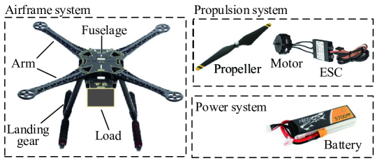
Figure 1: Typical compositions of multicopter body systems [2].

The design automation and optimization methodology can not only improve the design efficiency of the body system but also significantly shorten the development period of the entire multicopter system. The model-based development method [3, 4] is an efficient way to accelerate the development of control systems, but it requires a precise model of the multicopter, which depends on the body system design result. According to [5], designing the body system and control system of a UAV simultaneously is an efficient way in the future. Subsequently, the obtained multicopter system can be agile to respond to future changes in requirements.

Many optimization methods have been proposed for fixed-wing aircraft [6, 7] and helicopters [8], but the design optimization research for multicopters is scarce. Most studies focused on optimizing the designs of specific components (e.g., motors, propellers, airfoil shapes, and fuselage aerodynamics) to achieve longer flight endurance [9, 7, 10]. For example, a propeller efficiency analysis and optimization methods are studied in [11, 12], and a motor efficiency analysis and design methods are studied in [13]. However, according to [2], the efficiency of a multicopter is not only determined by the individual efficiency of a motor or a propeller, but also by many other factors such as the match between motors and propellers, the multicopter weight, and the flight conditions. For example, an unmatched propeller may make the motor work under a very inefficient state, which reduces the efficiency of the entire multicopter. In another example, an efficient multicopter may become very inefficient when the altitude (air density) or the payload weight are changed. Therefore, the multicopter should be treated as a whole to evaluate its performance and optimize its design.

In our earlier work [14], a practical method was proposed to estimate the flight performance of a multicopter with a given configuration, component selection, and flight conditions. This method allows designers to verify and update the multicopter design according to the estimated performance. The multicopter design optimization problem was essentially a reverse process of the performance estimation problem in [14]. In our latest work [15, 16], as the preliminary work of the design optimization problem, an analytic method was proposed to estimate the optimal parameters of propulsion systems in some simple design tasks. Based on our previous studies, this paper focuses on optimizing the multicopter as a whole by considering more practical factors. The study in this paper is more difficult and meaningful than our previous studies because the solution to the reverse process is not analytical and must correspond to real products and flight constraints.

A feasible way to solve the multicopter design optimization problem is to use numerical searching methods to traverse all possible design combinations and find the optimal one according to the objective functions and constraints. For example, in [17, 18], the multicopter optimization problem was described as a mixed-integer linear program and solved with the CPLEX optimizer. In [19], the design optimization problem was solved based on discrete-integer and continuous variables with the objectives of efficiency and flight time. In [20], based on knowledge-based engineering techniques, a design method was proposed to find a multicopter design with the minimum cost and maximum payload.

However, there exist some common problems with these methods. First, the calculation speed is slow owing to the large computational cost of traversing most of the possible combinations, especially when the product database is large. For example, it took 5–25 s to find the optimal design using a small-scale database (five motors and five propellers) for the methods in [17, 18]. However, in practice, a large product database is essential to cover common multicopters with different weights and sizes, which means that hours or days are required for these methods to obtain a reasonable result. Second, the performance of the obtained designs is calculated by theoretical estimation whose precision highly depends on the modeling accuracy and parameter precision. Third, the user requirements and optimization constraints considered in these papers are not comprehensive, so it is difficult to use the obtained results to assemble a real multicopter.

For the disadvantages of the existing methods, in this paper, a practical method is proposed to solve the multicopter design optimization problem with high computation speed and precision. The method contains two algorithms: an offline algorithm and an online algorithm. The offline algorithm finds the optimal components (propeller and ESC) for each motor to obtain motor-ESC-propeller propulsion combinations. Subsequently, all obtained propulsion combinations and their key performance parameters are stored in a combination database. The online algorithm obtains the multicopter design results that satisfy the given requirements by searching through component combinations in the database and calculating the optimal parameters for the battery and airframe. Subsequently, these requirement-satisfied multicopter design results are evaluated and sorted according to an objective function that contains evaluation indexes including size, weight, performance, and practicability. Finally, the optimal multicopter design is obtained according to the sorted list.

Compared with other methods, the advantages of the proposed method are as follows. (1) The calculation speed of the proposed method is much faster because most of the time-consuming calculations are completed offline. (2) The precision is higher because the parameters of the combination database can be calibrated by experimental data. (3) The obtained results are more practical because more design requirements and constraints are considered in our method.

The proposed method is beneficial for improving the development speed and reducing the cost of the design and verification of multicopters. Experiments and comparisons demonstrate the effectiveness and practicality of the proposed method. In addition, the method was published as an online toolbox to provide users with a multicopter optimization design service, and feedback indicates that the obtained results are accurate and practical for multicopter designs.

The rest of the paper is organized as follows. Section 2 provides a comprehensive description of the multicopter design optimization problem. In Section 3, the offline algorithm is presented to obtain a database with the optimal propulsion combinations. In Section 4, the online algorithm is presented to obtain the optimal multicopter design. Experiments and comparisons are discussed in Section 5. Section 6 presents the conclusions and future work.

2 Problem Formulation

This section presents the multicopter design optimization problem from five aspects: inputs, outputs, constraints, objectives, and solving method.

2.1 Design Requirements

The design requirements define the desired performance of a multicopter under the given flight conditions. Based on a market survey of multicopters, six important factors are considered in this paper:

(1) Hovering Time. The hovering time $\hat{t}_{\text{fly}}$ (unit: min) is defined as the battery discharge time in the hovering mode, in which the multicopter stays fixed in the air, and relatively static to the ground.

(2) Payload Capability. The payload weight $\hat{m}_{\text{load}}$ (unit: kg) describes the capacity to carry an instrument for certain missions.

(3) Maneuverability. The maneuverability usually refers to the acceleration ability, which is described by the thrust ratio $\hat{\gamma}\in\left(0,1\right)$ as

$$\hat{\gamma}\triangleq\frac{T_{\text{hover}}}{T^{*}}$$ (1)

where $T_{\text{hover}}$ (unit: N) is the hovering thrust of a single propeller in the hovering mode, and $T^{*}$ (unit: N) is the full-throttle thrust of a single propeller in the maximum control mode. According to the force balance principle, the total propeller thrust is equal to the multicopter weight in the hovering mode, which gives

$$n_{\text{p}}\cdot T_{\text{hover}}=m_{\text{copter}}\cdot g$$ (2)

where $m_{\text{copter}}$ (unit: kg) is the multicopter mass, $g=9.8\text{m/s}^{2}$ is the acceleration of gravity and $n_{\text{p}}$ is the number of propellers. Meanwhile, the vertical acceleration range of a multicopter is $\left[-g,a_{\text{vMax}}\right]$, where $-g$ denotes the acceleration in the free fall motion when all propellers stop rotating, and $a_{\text{vMax}}$ (unit: m/$\text{s}^{2}$) denotes the maximum vertical acceleration when all propellers generate the full-throttle thrust $T^{*}$. According to Eqs. (1) and (2), $a_{\text{vMax}}$ is obtained as

$$a_{\text{vMax}}=\frac{n_{\text{p}}T^{*}-m_{\text{copter}}g}{m_{\text{copter}}}=\left(\frac{1}{\hat{\gamma}}-1\right)g.$$ (3)

It can be observed from Eq. (3) that the acceleration range (maneuverability) is directly determined by the thrust ratio $\hat{\gamma}$. In practice, multicopters with different usages have different maneuverability preferences. For example, racing multicopters expect a smaller thrust ratio $\hat{\gamma}$ for higher maneuverability, while load-carrying multicopters expect a larger $\hat{\gamma}$ to allocate more weight for payload. In particular, when $\hat{\gamma}=0.5$, the acceleration range obtained from Eq. (3) is $\left[-g,g\right]$, which is widely adopted by designers because it has the most balanced control range. Moreover, according to [14, 21], the maximum flight speed of a multicopter can also be obtained by the thrust ratio $\hat{\gamma}$ with the given aerodynamic coefficients.

(4) Airframe Layout. According to [2], multicopter airframe layouts can usually be divided into common layouts and coaxial layouts. Fig. 2 shows several basic airframe layouts for multicopters, where Figs. 2(a)(b)(c) are of the common form and Figs. 2(a)(b)(c) are of the coaxial form. For common multicopters, the propeller number $n_{\text{p}}$ is equal to the arm number, and the propellers are assumed not to interfere with each other. For coaxial multicopters, there are two propellers on the same arm, and the propeller thrust efficiency may decrease by about 20% owing to the interaction between propellers [2]. This paper studies the design for common-layout multicopters, and the proposed method can be easily applied to the coaxial layout or other special layouts.

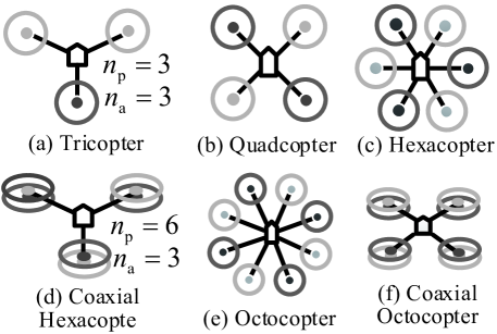
Figure 2: Basic airframe layouts for multicopters.

(5) Air Density (Altitude). The air density $\hat{\rho}$ (unit: kg/$\text{m}^{3}$) has a great influence on the performance of a multicopter. For example, most multicopters cannot even take off in high-altitude areas because the thrust becomes much smaller than that in sea-level areas owing to the reduction of air density. According to the international standard atmosphere (ISA) statistical model [22], the air density can be estimated by the altitude $h_{\text{t}}$ (unit: m) as

$$\begin{array}[]{cl}\hat{\rho}&\approx\frac{273}{(273+T_{\text{t}})}(1-0.0065\frac{h_{\text{t}}}{273+T_{\text{t}}})^{5.2561}\rho_{\text{0}}\\ T_{\text{t}}&\approx T_{\text{0}}-\left(6\cdot h_{\text{t}}/1000\right)\end{array}$$ (4)

where $\rho_{\text{0}}=1.293$kg/m³ is the standard air density, $T_{\text{t}}$ (unit: ^∘C) is the air temperature, and $T_{\text{0}}=25{}^{\circ}\text{C}$ is the average ground temperature.

(6) Battery Type (Power Density). The power density $\rho_{\text{b}}$ (unit: W$\cdot$h/kg) determines the battery weight under the same capacity. Although a battery with a higher power density is always better in multicopter design, in practice, the selection of the battery also depends on other factors such as safety, cost, and performance. For a certain type of battery product, the power density is approximately equal to a constant value. For example, for the most commonly used Li-Po batteries, the power density is $\rho_{\text{b}}$$\approx 240$W$\cdot$h/kg.

For simplicity, the above design requirements are marked with an input parameter set $\mathbf{\Theta}_{\text{in}}$ as

$$\mathbf{\Theta}_{\text{in}}\triangleq\left\{\hat{t}_{\text{fly}},\hat{m}_{\text{load}},\hat{\gamma},n_{\text{p}},\hat{\rho},\rho_{\text{b}}\right\}.$$ (5)

2.2 Design Outputs

The design outputs contain all necessary information to assemble a multicopter.

(1) Product Selection of Propulsion System. It is expected that the proposed method can comprehensively determine the product selection (motor, ESC, and propeller) of the propulsion system. Therefore, a certain number of candidate products is necessary to be prepared as the searching scope. For simplicity, the name and parameters (e.g., size, weight, and current limit) of a motor product are marked with a parameter set $\Theta_{\text{m}}$. The motor database, which includes all available motor products, is represented by a symbol $\mathbf{\Phi}_{\text{m}}$, where $\Theta_{\text{m}}\in\mathbf{\Phi}_{\text{m}}$. Similar definitions are applied to ESCs $\Theta_{\text{e}}\in\mathbf{\Phi}_{\text{e}}$ and propellers $\Theta_{\text{p}}\in\mathbf{\Phi}_{\text{p}}$. Next, a propulsion system combination can be represented by $\left\{\Theta_{\text{m}},\Theta_{\text{e}},\Theta_{\text{p}}\right\}$.

(2) Battery Parameters. The battery pack is a highly customizable component. Users can connect many small battery cells in serial and parallel to obtain the desired voltage and capacity. The basic battery parameters include the nominal voltage $U_{\text{b}}$ (unit: V), capacity $C_{\text{b}}$ (unit: mAh) and maximum discharge current $I_{\text{bMax}}$ (unit: A).

(3) Airframe Diameter. The airframe diameter $D_{\text{air}}$ (unit: m) is defined as the diameter of the circle formed by the motors, which is necessary to design an airframe or select a suitable product on the market. For example, if the obtained airframe diameter is $D_{\text{air}}=0.45\text{m}$, then the popular airframe DJI F450 can be selected to assemble the multicopter.

(4) Actual Performance. The actual performance of the designed multicopter is necessary for users to evaluate the optimization effect. In this paper, the actual hovering time, payload weight and thrust ratio are represented by $\overline{t}_{\text{fly}},\overline{m}_{\text{load}},$ and $\overline{\gamma}$, respectively. The weight of the design multicopter is represented by $m_{\text{copter}}$ (unit: kg).

For simplicity, the above design outputs are marked with an output parameter set $\mathbf{\Theta}_{\text{out}}$ as

$$\mathbf{\Theta}_{\text{out}}\triangleq\left\{\Theta_{\text{m}},\Theta_{\text{e}},\Theta_{\text{p}},\overline{t}_{\text{fly}},\overline{m}_{\text{load}},\overline{\gamma},U_{\text{b}},C_{\text{b}},I_{\text{bMax}},D_{\text{air}},m_{\text{copter}}\right\}.$$ (6)

2.3 Optimization Constraints

The following constraints should be considered to ensure the safety and practicability of the obtained multicopter design.

(1) Requirement Constraint. The actual performance of the designed multicopter $\overline{t}_{\text{fly}},\overline{m}_{\text{load}},\overline{\gamma}\in\mathbf{\Theta}_{\text{out}}$ should be equal (or close) to the desired performance $\hat{t}_{\text{fly}},\hat{m}_{\text{load}},\hat{\gamma}\in\mathbf{\Theta}_{\text{in}}$.

(2) Safety Constraint. The voltages and currents of electronic components (motors, ESCs, and batteries) should work within the allowed range to avoid being burnt out.

(3) Compatibility Constraint. Compatibility is important during multicopter design. Components have to be compatible with each other or they cannot work properly or even fail in some cases. Incompatibilities often occur between ESCs and motors. Consequently, every motor product lists its compatible ESC products on its description page.

(4) Structure Constraint. The structure constraint determines the airframe design. If the airframe is too small, then the propellers may collide with each other.

2.4 Optimization Objectives

In practice, there is no uniform standard to evaluate the design of a multicopter. According to [19, 20], the multicopter design optimization problem is essentially a multiobjective optimization problem, so an “optimal design” should fully consider all factors concerned by designers and customers. Therefore, an objective function $J=f_{J}\left(\mathbf{\Theta}_{\text{out}}\right)$ is proposed in this paper to evaluate the obtained multicopter designs and find the optimal $\mathbf{\Theta}_{\text{out}}^{*}$.

Compared to the objective functions in [19, 20], two improvements are introduced in this paper. First, the normalization operation is applied to each evaluation index, which makes it easier to determine the weight factor according to the preferences of designers. Second, more evaluation indexes are considered in this paper according to actual applications. These evaluation indexes are as follows:

(1) Size and Weight. The size and weight are the most important factors for designers. A smaller and lighter multicopter is more portable and convenient for users.

(2) Requirement Agreement. The performance (hovering time, payload capability, and maneuverability) of the obtained multicopter should be as close as possible to the given design requirements.

(3) Efficiency. The efficiency should be as high as possible to consume less power under the same conditions.

(4) Practicability. For most users, the components of the multicopter design should be easy to find on the market.

(5) Safety Margin. The safety margin indicates that the full-throttle current of a propulsion system should maintain a certain distance based on its safety limit, which ensures that the multicopter works safely in a wider range of flight conditions.

2.5 Solving Method

In summary, the problem inputs are the product databases $\mathbf{\Phi}_{\text{m}},\mathbf{\Phi}_{\text{e}},\mathbf{\Phi}_{\text{p}}$ and design requirements $\mathbf{\Theta}_{\text{in}}$. The problem output is the optimal multicopter design $\mathbf{\Theta}_{\text{out}}^{*}$. Fig. 3 presents the key steps of the solving method in this paper. The detailed procedures in Fig. 3 will be presented in Section 3 (offline algorithm) and Section 4 (online algorithm).

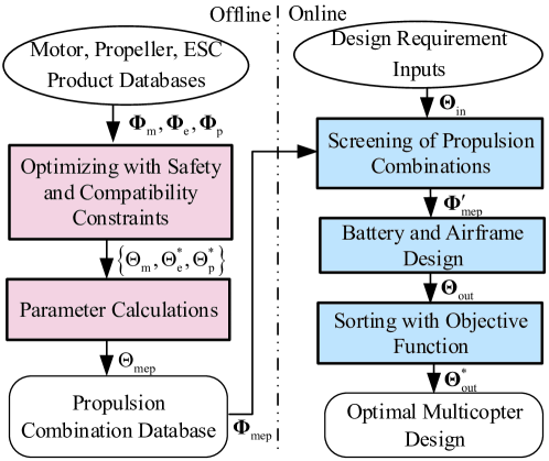
Figure 3: Framework of the optimization design method.

3 Offline Propulsion System Optimization

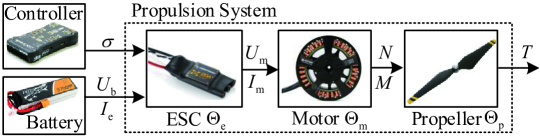
Figure 4: Connection and power consumption of a propulsion system.

Fig. 4 shows the component connection and power consumption of a propulsion system. The power of a propulsion system is provided by the battery whose input voltage and current are represented by $U_{\text{b}}$ (unit: V) and $I_{\text{e}}$ (unit: A) respectively. The flight controller sends the throttle control signal $\sigma\in\left[0,1\right]$ to ESC, and then ESC generates a PWM-modulated signal to control the propeller rotating speed $N$ (unit: RPM) to get the desired thrust $T$ (unit: N). With the throttle signal $\sigma$ increasing from 0 to 1 (full throttle), the values of $T$,$I_{\text{e}}$,$N$ increase from 0,0,0 to their full-throttle maximum values $T^{*},I_{\text{e}}^{*},N^{*}$.

3.1 Optimal propulsion Combination

3.1.1 Evaluation Indexes

In practice, the full-throttle thrust $T^{*}$, the thrust efficiency $\eta^{\text{t}}$ (unit: N/W) and the total weight $m_{\text{mep}}$ (unit: kg) are three most concerned evaluation indexes for propulsion systems. The thrust efficiency $\eta^{\text{t}}$ is defined as the ratio between the instantaneous output thrust $T$ and ESC input power $P_{\text{e}}$

$$\eta^{\text{t}}\triangleq\frac{T}{P_{\text{e}}}=\frac{T}{U_{\text{b}}\cdot I_{\text{e}}}.$$ (7)

where $U_{\text{b}}$ (unit: V) is the battery voltage, and $I_{\text{e}}$ is the instantaneous ESC input current. A higher thrust efficiency $\eta^{\text{t}}$ indicates a lower input power $P_{\text{e}}$ for generating the same thrust $T$, which leads to longer hovering time. Noteworthy, the thrust efficiency $\eta^{\text{t}}$ is not a constant value, and it changes with the throttle $\sigma$. Therefore, the full-throttle thrust efficiency $\eta^{\text{t*}}=T^{*}/\left(U_{\text{b}}I_{\text{e}}^{*}\right)$ is usually adopted to evaluate the efficiency of a propulsion system.

3.1.2 Objective Function

The objective function to evaluate a motor-ESC-propeller propulsion combination is given by

$$\begin{array}[]{cl}J_{\text{mep}}&=f_{J_{\text{mep}}}\left(\Theta_{\text{m}},\Theta_{\text{e}},\Theta_{\text{p}}\right)\\ &=k_{\text{m}1}\cdot\frac{T^{*}}{\overline{T}^{*}}+k_{\text{m}2}\cdot\frac{\eta^{\text{t*}}}{\overline{\eta}^{\text{t*}}}+k_{\text{m}3}\cdot\frac{-m_{\text{mep}}}{\overline{m}_{\text{mep}}}\end{array}$$ (8)

where $\overline{T}^{*},\overline{\eta}^{\text{t*}},\overline{m}_{\text{mep}}$ are normalization parameters, and $k_{\text{m}1},k_{\text{m}2},k_{\text{m}3}$ are weight factors. The normalization parameter $\overline{T}^{*}$ is defined as the maximum full-throttle thrust $T^{*}$ among all obtained combinations. The same definitions are applied to the normalization parameters $\overline{\eta}^{\text{t*}},\overline{m}_{\text{mep}}.$ The parameters $k_{\text{m}1},k_{\text{m}2},k_{\text{m}3}$ are positive coefficients specified by designers according to design preferences. Usually, $\left\{k_{\text{m}1},k_{\text{m}2},k_{\text{m}3}\right\}=\left\{1,1,1\right\}$ can be selected if there is no special requirement. A better propulsion combination should have larger $J_{\text{mep}}$ which indicates larger output thrust $T^{*}$, higher efficiency $\eta^{\text{t*}}$ and lighter weight $m_{\text{mep}}$. Noteworthy, more evaluation indexes (cost, size, etc.) can also be included in $J_{\text{mep}}$ in Eq. (8) according to the actual demand.

3.1.3 Constraints

The safety constraint for a propulsion system denotes that the voltage and current of motors and ESCs should not exceed their allowable limits for safe operation, which can be described as

$$\begin{array}[]{c}I_{\text{e}}^{*}\leq I_{\text{mMax}},I_{\text{e}}^{*}\leq I_{\text{eMax}}\\ U_{\text{b}}\leq U_{\text{mMax}},U_{\text{b}}\leq U_{\text{eMax}}\end{array}$$ (9)

where $I_{\text{mMax}},U_{\text{mMax}}\in\Theta_{\text{m}}$ and $I_{\text{eMax}},U_{\text{eMax}}\in\Theta_{\text{e}}$ denote the current and voltage upper limits of the motor and the ESC respectively.

The compatibility constraint requires that the propulsion components (motor, ESC and propeller) should be compatible with each other. Since manufacturers will list the compatible products on product websites, using a lookup table to store these compatible relationships among components is a possible way to describe the compatibility constraint. For example, a compatibility judging function $f_{\text{tab}}\left(\Theta_{\text{m}},\Theta_{\text{e}},\Theta_{\text{p}}\right)$ can be obtained based on the lookup table to describe the compatible constraint as

$$f_{\text{tab}}\left(\Theta_{\text{m}},\Theta_{\text{e}},\Theta_{\text{p}}\right)=\begin{cases}\text{false},&\text{incompatible}\\ \text{true},&\text{compatible}\end{cases}.$$ (10)

Remark 1. Considering that the products from the same manufacturer will be compatible with each other, a more convenient way to avoid the compatibility problem is to select the motor, ESC and propeller products from the same manufacturer.

3.1.4 Brute Force Searching Method

The brute force searching algorithm is described as follows.

 

Algorithm 1 Brute force searching algorithm for optimal propulsion combination

 

Step 1: For each motor $\Theta_{\text{m}}$ in the motor database $\mathbf{\Phi}_{\text{m}}$, traverse all ESC and propeller products in the databases $\mathbf{\Phi}_{\text{e}},\mathbf{\Phi}_{\text{p}}$ to screen out the motor-ESC-propeller combinations $\left\{\Theta_{\text{m}},\Theta_{\text{e}},\Theta_{\text{p}}\right\}$ that satisfy the constraints in Eqs. (9)(10).

Step 2: Obtain the values of $U_{\text{b}},I_{\text{e}}^{*},T^{*},m_{\text{mep}},\eta^{\text{t*}}$ for each combination {$\Theta_{\text{m}},\Theta_{\text{e}},\Theta_{\text{p}}$} through experimental measurement or theoretical estimation in [14].

Step 3. Obtain the normalization parameters $\overline{T}^{*},\overline{\eta}^{\text{t*}},\overline{m}_{\text{mep}}$ by finding the maximum values of $T^{*},\eta^{\text{t*}},m_{\text{mep}}$ from results in Step 2.

Step 4: Calculate the objective function $J_{\text{mep}}$ for each combination, and select the combination with the maximum $J_{\text{mep}}$ as the optimal combination ${\Theta_{\text{m}},\Theta_{\text{e}}^{*},\Theta_{\text{p}}^{*}}$, where ${\Theta_{\text{e}}^{*},\Theta_{\text{p}}^{*}}=\text{argmax}_{\Theta_{\text{e}},\Theta_{\text{p}}}f_{J_{\text{mep}}}\left(\Theta_{\text{m}},\Theta_{\text{e}},\Theta_{\text{p}}\right).$

Step 5: Repeat the above procedures for all motors $\Theta_{\text{m}}$ in database $\mathbf{\Phi}_{\text{m}}$, and a series of propulsion combinations ${\Theta_{\text{m}},\Theta_{\text{e}}^{*},\Theta_{\text{p}}^{*}}_{k}$ can be obtained.

 

3.1.5 Analytical Solution Method

In our previous work [15], an analytical method is proposed to find an optimal propulsion combination {$\Theta_{\text{m}}$,$\Theta_{\text{e}}^{*}$,$\Theta_{\text{p}}^{*}$} according to the given full-throttle thrust requirement $T^{*}$. Therefore, by giving a series of $T^{*}$ with values varying from 0.1N to 100N, the optimization method in [15] can output a series of propulsion combinations {$\Theta_{\text{m}}$,$\Theta_{\text{e}}^{*}$,$\Theta_{\text{p}}^{*}$}_k that are capable of covering most common multicopters with normal size and weight.

3.1.6 Experimental Selection Method

Since most manufacturers will publish the motor test data with the recommended ESC and propeller products, selecting the optimal combination through these test data is a more convenient and precise way to obtain the combination database $\mathbf{\Phi}_{\text{mep}}$. For example, Fig. 5 demonstrates the product parameters and test results of motor MN3508 KV380 on the T-MOTOR website [23], where the recommend two propeller products are 14$\times$4.8CF (Diameter: 14 inches, Pitch: 4.8 inches, Weight: 19.2g) and 15$\times$5CF (Diameter: 15 inches, Pitch: 5 inches, Weight: 26.5g), and the recommend ESC product is AIR 40 (Maximum Voltage: 22.2V, Maximum Current: 40A, Weight: 26g). Therefore, there are two combinations that can be obtained from Fig. 5, and the latter one is selected as the optimal combination according to Eq. (8), namely {$\Theta_{\text{m}}$,$\Theta_{\text{e}}^{*}$,$\Theta_{\text{p}}^{*}$}={MN3508 KV380, 15$\times$5CF, AIR 40}. Since the combination has been tested and verified through experiments, the safety and compatibility constraints are strictly satisfied, and the combination is practical enough to be applied to assemble a real multicopter.

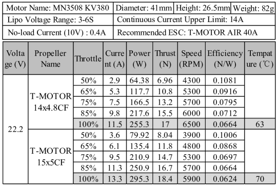
Figure 5: Product specification and experimental test data of T-MOTOR MN3508 KV380 [23].

3.2 Parameter Calculation

After getting the optimal ESC and propeller for a certain motor, some parameters are required for the subsequent online design optimization algorithm including Battery Voltage: $U_{\text{b}}$ (unit: V); Propeller Diameter: $D_{\text{p}}$ (unit: m); Motor KV Value $K_{\text{V}}$ (unit: RPM/V); Total Weight: $m_{\text{mep}}$ (unit: kg); Full-throttle Thrust: $T^{*}$ (unit: N); Full-throttle Speed: $N^{*}$ (unit: RPM); Full-throttle Current: $I_{\text{e}}^{*}$ (unit: A); Air Density: $\rho$ (unit: kg/$\text{m}^{3}$); Motor Nominal Maximum Current $I_{\text{mMax}}$ (unit: A). The above parameters can be directly obtained from the experimental test data as shown in Fig. 5 or calculated with the estimation method in our previous work [14]. The air density $\rho$ can be estimated by Eq. (4) according to the altitude $h_{\text{t}}$ of the experimental location.

According to [14], the relationship between the output thrust $T$ (unit: N) and the input current $I_{\text{e}}$ (unit: A) (thrust-current curve) of a propulsion combination is very important for estimating the performance of a multicopter, but it is very complex and highly nonlinear which requires very accurate parameters and large computational cost. In order to simplify the computation, the curve fitting method is adopted to approximate the thrust-current curve in this paper. Since the curve fitting is finished offline and the results can be calibrated through experimental test data, the computation speed and precision of the online multicopter design optimization algorithm are significantly improved compared with the previous methods. According to our statistic analysis, the second-order polynomial fitting method is highly effective in approximating the thrust-current curve of propulsion combinations, which is given by

$$I_{\text{e}}=f_{\text{IT}}\left(T\right)=k_{\text{t2}}\cdot T^{2}+k_{\text{t1}}\cdot T+k_{\text{t0}}$$ (11)

where $k_{\text{t0}},k_{\text{t1}},k_{\text{t2}}$ are constant values obtained by curve fitting. For example, the curve fitting results for the test data from Fig. 5 are presented in Fig. 6. It can be observed from the figure that both Adjusted R-square values are larger than 0.99, which indicates that the second-order polynomial function in Eq. (11) can express the thrust-current curve of a propulsion system in high precision.

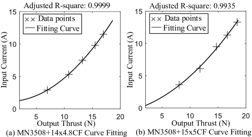
Figure 6: Second-order polynomial curve fitting results for current-thrust data of motor MN3508.

3.3 Database Generation

The combination {$\Theta_{\text{m}},\Theta_{\text{e}}^{*},\Theta_{\text{p}}^{*}$} along with the necessary parameters are represented by a parameter set $\Theta_{\text{mep}}$ as

$$\begin{array}[]{ll}\Theta_{\text{mep}}\triangleq&\left\{\Theta_{\text{m}},\Theta_{\text{e}}^{*},\Theta_{\text{p}}^{*},U_{\text{b}},D_{\text{p}},K_{\text{V}},m_{\text{mep}},\right.\\ &\left.T^{*},N^{*},I_{\text{e}}^{*},I_{\text{mMax}},\rho,k_{\text{t2}},k_{\text{t1}},k_{\text{t0}}\right\}\end{array}.$$

For example, the optimal propulsion combination for motor MN3508 KV380 obtained from Fig. 5 is $\Theta_{\text{mep}}=${MN3508 KV380, 15$\times$5CF, AIR 40, 22.2, 0.381, 380, 134.5, 18.4, 5900, 13.3, 14, 1.2, 0.0262, 0.2559, -0.2349}. By applying the optimal combination method for each motor, a propulsion combination database $\mathbf{\Phi}_{\text{mep}}$ can be obtained with $\Theta_{\text{mep}}\in\mathbf{\Phi}_{\text{mep}}$. The online algorithm will traverse all the combinations $\Theta_{\text{mep}}$ in $\mathbf{\Phi}_{\text{mep}}$ to find the optimal solution for the desired multicopter.

Remark 2. In practice, it is unnecessary to include all the products on the market to build the database $\mathbf{\Phi}_{\text{mep}}$ because products with similar specifications have similar performance. According to our practical experience, it is adequate to design common multicopters (weight range: 0.1kg $\sim$ 50kg) by using a combination database $\mathbf{\Phi}_{\text{mep}}$ with less than 1000 items. Of course, professional users can also include their self-designed products into $\mathbf{\Phi}_{\text{mep}}$ to improve the current multicopter design.

4 Online Multicopter Design Optimization

In this section, for each combination $\Theta_{\text{mep}}\in\mathbf{\Phi}_{\text{mep}}$, the battery and airframe will be designed according to the design requirements $\mathbf{\Theta}_{\text{in}}$ to obtain a multicopter design $\mathbf{\Theta}_{\text{out}}$. Then, an objective function is proposed to evaluate these multicopter designs to find the optimal solution $\mathbf{\Theta}_{\text{out}}^{*}$.

4.1 Selection of Propulsion Combinations

4.1.1 Weight Decomposition

The total weight of a multicopter $m_{\text{copter}}$ (unit: kg) is given by

$$m_{\text{copter}}=\hat{m}_{\text{load}}+m_{\text{airframe}}+m_{\text{battery}}+n_{\text{p}}\cdot m_{\text{mep}}$$ (12)

where $\hat{m}_{\text{load}}\in\mathbf{\Theta}_{\text{in}}$ is the desired payload weight, $m_{\text{airframe}}$ (unit: kg) is the airframe weight (includes flight controller and other instruments), $m_{\text{battery}}$ (unit: kg) is the battery weight, $m_{\text{mep}}\in\Theta_{\text{mep}}$ is the weight of a propulsion combination, $n_{\text{p}}\in\mathbf{\Theta}_{\text{in}}$ is the propeller number. Since an airframe is used to support the whole multicopter weight $m_{\text{copter}}$, according to the statistical analysis in [24], its weight $m_{\text{airframe}}$ is usually proportional to $m_{\text{copter}}$ as

$$m_{\text{airframe}}=\alpha_{\text{air}}\cdot m_{\text{copter}}$$ (13)

where the airframe weight ratio $\alpha_{\text{air}}$ may vary from 0.08 to 0.40 for multicopters with different materials and structures. An average value $\alpha_{\text{air}}=0.19$ is suggested in [24] for common multicopters. Meanwhile, by substituting the full-throttle thrust $T^{*}\in\Theta_{\text{mep}}$ and the input parameters $\hat{\gamma},n_{\text{p}}\in\mathbf{\Theta}_{\text{in}}$ into Eqs. (1)(2), the multicopter weight $m_{\text{copter}}$ is obtained as

$$T_{\text{hover}} =\hat{\gamma}\cdot T^{*}$$ (14)

$$m_{\text{copter}} =\frac{n_{\text{p}}\cdot T_{\text{hover}}}{g}=\frac{n_{\text{p}}\cdot\hat{\gamma}\cdot T^{*}}{g}.$$ (15)

Finally, by combining Eqs. (12)(13)(15), the battery weight $m_{\text{battery}}$ is obtained as

$$m_{\text{battery}}=\left(1-\alpha_{\text{air}}\right)m_{\text{copter}}-\hat{m}_{\text{load}}-n_{\text{p}}\cdot m_{\text{mep}}.$$ (16)

Remark 3. The full-throttle thrust $T^{*}$ is determined by the air density $\rho$. Therefore, if the desired air density $\hat{\rho}\in\mathbf{\Theta}_{\text{in}}$ is not equal to the default air density $\rho$ in $\Theta_{\text{mep}}$, conversion has to be made to obtain the actual full-throttle thrust $\overline{T}^{*}$ in Eqs. (15)(15). Based on the mathematical model of propulsion systems in Appendix A, the conversion method to obtain $\overline{T}^{*}$ is derived in Appendix B.

4.1.2 Battery Hovering Current Calculation

Assuming that the multicopter is in hovering mode, by substituting Eq. (14) into Eq. (11) with $T=T_{\text{hover}}$, the hovering input current of a propulsion combination $I_{\text{eHover}}$ (unit: A) is given by

$$\begin{array}[]{c}I_{\text{eHover}}=k_{\text{t0}}+k_{\text{t1}}\cdot T_{\text{hover}}+k_{\text{t2}}\cdot T_{\text{hover}}^{2}\end{array}.$$ (17)

Then, the battery hovering current $I_{\text{bHover}}$ (unit: A) is obtained as

$$I_{\text{bHover}}=n_{\text{p}}\cdot I_{\text{eHover}}+I_{\text{other}}$$ (18)

where $n_{\text{p}}\cdot I_{\text{eHover}}$ denotes the total current of all motors, and $I_{\text{other}}$ (unit: A) denotes other current consumption such as the current of the flight controller. According to [14], a statistic value $I_{\text{other}}\approx 0.5$A can be applied for the approximate calculation if $I_{\text{other}}$ is unknown.

Remark 5. As mentioned before, if the desired air density $\hat{\rho}\in\mathbf{\Theta}_{\text{in}}$ is different from the default air density $\rho$ in $\Theta_{\text{mep}}$, conversion has to be made to obtain the actual input current $\overline{I}_{\text{eHover}}$ in Eq. (17), where the conversion method is presented in Appendix C.

4.1.3 Discharge Time Calculation

The definition of the battery power density $\rho_{\text{b}}$ (unit: W$\cdot$h/kg) is given by

$$\rho_{\text{b}}\triangleq\frac{U_{\text{b}}\cdot I_{\text{bHover}}\cdot t_{\text{dis}}/60}{m_{\text{battery}}}$$ (19)

where $t_{\text{dis}}$ (unit: min) is the total discharge time of a battery, and $U_{\text{b}}\in\Theta_{\text{mep}}$ is the battery voltage. In practice, a part of the capacity should be retained to protect the battery from over-discharging. Therefore, the actual battery discharge time $\overline{t}_{\text{dis}}$ is given by

$$\overline{t}_{\text{dis}}=\alpha_{\text{b}}t_{\text{dis}}=\alpha_{\text{b}}\frac{60\cdot\rho_{\text{b}}m_{\text{battery}}}{U_{\text{b}}\cdot I_{\text{bHover}}}$$ (20)

where $\alpha_{\text{b}}\in\left(0,1\right)$ is the discharge capacity ratio. According to [14], an average value $\alpha_{\text{b}}$$\approx$0.9 can be applied for the approximate calculation if $\alpha_{\text{b}}$ is unknown.

4.1.4 Selection for Design Requirements

Ideally, the battery discharge time $\overline{t}_{\text{dis}}$ obtained from Eq. (20) should be equal to the desired hovering time $\hat{t}_{\text{fly}}\in\mathbf{\Theta}_{\text{in}}$, which can ensure that the design requirements described by parameters $\hat{m}_{\text{load}},\hat{\gamma},\hat{t}_{\text{fly}}$ are satisfied simultaneously. However, in practice, it is too strict to find a combination $\Theta_{\text{mep}}$ from database $\mathbf{\Phi}_{\text{mep}}$ that exactly satisfies all requirements $\overline{t}_{\text{dis}}=\hat{t}_{\text{fly}},\overline{m}_{\text{load}}=\hat{m}_{\text{load}},\overline{\gamma}=\hat{\gamma}$. Therefore, the following selection criterion is proposed to evaluate whether the propulsion combination satisfies the design requirements within the tolerable error as

$$\left|\frac{\overline{t}_{\text{dis}}-\hat{t}_{\text{fly}}}{\hat{t}_{\text{fly}}}\right|\leq\varepsilon_{\text{t}}$$ (21)

where $\varepsilon_{\text{t}}$ is a small positive threshold specified by designers according to the tolerance for design error. If the selection criterion in Eq. (21) is satisfied for a motor-ESC-propeller combination $\Theta_{\text{mep}}$, the actual performance of the multicopter designed based on $\Theta_{\text{mep}}$ is given by

$$\overline{t}_{\text{fly}}=\overline{t}_{\text{dis}}\approx\hat{t}_{\text{fly}},\overline{m}_{\text{load}}=\hat{m}_{\text{load}},\overline{\gamma}=\hat{\gamma}.$$ (22)

In summary, the screening algorithm to find the propulsion combinations that satisfy the given design requirements are listed as follows.

 

Algorithm 2 Screening algorithm for requirement-satisfied combinations

 

Step 1: For a combination $\Theta_{\text{mep}}$ in database $\mathbf{\Phi}_{\text{mep}}$, the discharge time $\overline{t}_{\text{dis}}$ can be obtained by substituting parameter sets $\Theta_{\text{mep}}$ and $\mathbf{\Theta}_{\text{in}}$ into Eqs. (15)-(20).

Step 2: If the obtained $\overline{t}_{\text{dis}}$ satisfies the screening criterion in Eq. (21), then store this combination $\Theta_{\text{mep}}$ into a database which is marked as $\mathbf{\Phi}_{\text{mep}}^{\prime}$.

Step 3: Repeat the above two steps for all combinations $\Theta_{\text{mep}}$ in $\mathbf{\Phi}_{\text{mep}}$, and a database $\mathbf{\Phi}_{\text{mep}}^{\prime}$ is obtained for the following design and optimization procedures. If no combination is obtained, then an error should be emitted to stop the whole optimization program.

 

Remark 6. The selection criterion in Eq. (21) can also be formulated based on the errors of $\hat{m}_{\text{load}}$ or $\hat{\gamma}$ instead of $\hat{t}_{\text{fly}}$, which provides similar selection effect.

4.2 Battery and Airframe Design

4.2.1 Battery Design

The basic battery parameters that determine a battery product include the nominal voltage $U_{\text{b}}$ (unit: V), the capacity $C_{\text{b}}$ (unit: mAh) and the maximum discharge current $I_{\text{bMax}}$ (unit: A). First, the battery voltage $U_{\text{b}}$ can be obtained from parameter set $\Theta_{\text{mep}}$. Secondly, according to Eq. (18), the full-throttle battery discharge current is obtained as $I_{\text{b}}^{*}=n_{\text{p}}\cdot I_{\text{e}}^{*}+I_{\text{other}}$, where $I_{\text{e}}^{*}\in\Theta_{\text{mep}}$ is the full-throttle current of a propulsion system. It is required that $I_{\text{bMax}}\geq I_{\text{b}}^{*}$ for the safe operation of batteries. With necessary safety margin, the battery maximum discharge current $I_{\text{bMax}}$ is obtained as

$$I_{\text{bMax}}=\alpha_{\text{Ib}}\cdot I_{\text{b}}^{*}=\alpha_{\text{Ib}}\cdot\left(n_{\text{p}}\cdot I_{\text{e}}^{*}+I_{\text{other}}\right)$$ (23)

where usually $\alpha_{\text{Ib}}\geq 1.5$. Thirdly, according to the definition of the battery capacity with unit mAh, the battery $C_{\text{b}}$ is obtained as

$$C_{\text{b}}=1000\cdot I_{\text{bHover}}\frac{\overline{t}_{\text{fly}}/\alpha_{\text{b}}}{60}$$ (24)

where $I_{\text{bHover}}$ and $\alpha_{\text{b}}$ are presented in Eq. (18)(20). Thus, the battery parameters $U_{\text{b}},I_{\text{bMax}},C_{\text{b}}$ are obtained for the output parameter set $\Theta_{\text{out}}$.

4.2.2 Airframe Design

The airframe diameter $D_{\text{air}}$ (unit: m) is the most important parameter in designing or selecting an airframe product. In practice, $D_{\text{air}}$ (unit: m) is expected to be as small as possible. However, the propellers may interfere with each other if $D_{\text{air}}$ is too small. Fig. 7 shows the minimum airframe radius $R_{\text{min}}$ for different types of multicopters, where $R_{\text{p}}=D_{\text{p}}/2$ is the propeller radius, $R_{\text{air}}=D_{\text{air}}/2$ is the airframe radius, $\theta_{\text{r}}=2\pi/n_{\text{r}}$ is the angle (unit: rad) between adjacent arms, and $n_{\text{r}}$ is the number of arms. Therefore, according to the geometrical relationship in Fig. 7, the minimum airframe radius $R_{\text{min}}$ is given by

$$R_{\text{air}}\geq R_{\text{min}}=\frac{R_{\text{p}}}{\sin\left(\frac{\theta_{\text{r}}}{2}\right)}=\frac{D_{\text{p}}}{2\sin\left(\pi/n_{\text{r}}\right)}.$$ (25)

Although the constraint $R_{\text{air}}\geq R_{\text{min}}$ can avoid physical interference between two adjacent propellers, the aerodynamic interference still exists when two propellers are too close to each other [25]. Therefore, necessary gap is required between adjacent propellers, so the optimal airframe diameter $D_{\text{air}}$ can be selected as

$$D_{\text{air}}=2R_{\text{air}}=2\alpha_{\text{r}}\cdot R_{\text{min}}=\frac{2\alpha_{\text{r}}D_{\text{p}}}{2\sin\left(\pi/n_{\text{r}}\right)}$$ (26)

where $\alpha_{\text{r}}=1.05\sim 1.2$ is suggested in [2, p. 62].

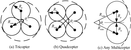
Figure 7: Minimum airframe for multicopter design.

4.3 Evaluation, Ordering and Optimization

Repeating the above procedures for all combinations $\Theta_{\text{mep}}$ in database $\mathbf{\Phi}_{\text{mep}}^{\prime}$, their corresponding airframe and battery parameters can be obtained according to the requirement and structure constraints. As a result, a series of multicopter designs $\Theta_{\text{out}}$ defined in Eq. (6) are obtained. In this subsection, an objective function $J=f_{J}\left(\Theta_{\text{out}}\right)$ is proposed to evaluate these multicopter designs $\Theta_{\text{out}}$. The one with the minimum $J$ will be selected as the optimal multicopter design $\Theta_{\text{out}}^{*}$.

The objective function $f_{J}\left(\Theta_{\text{out}}\right)$ is given by

$$J=f_{J}\left(\Theta_{\text{out}}\right)=\sum_{i=1}^{7}k_{i}\frac{X_{i}}{\overline{X}_{i}}$$ (27)

where $X_{1},\cdots,X_{7}\in\mathbb{R^{\mathnormal{+}}}$ are evaluation indexes, $\overline{X}_{1},\cdots,\overline{X}_{7}\in\mathbb{R^{\mathnormal{+}}}$ are normalizing parameters, and $k_{1},\cdots,k_{7}\in\mathbb{R^{\mathnormal{+}}}$ are weight factors. The detailed definitions are given below

$$X_{1} =D_{\text{air}},X_{2}=m_{\text{copter}},$$

$$X_{3} =\begin{array}[]{c}\sqrt{\left(\frac{\overline{t}_{\text{fly}}-\hat{t}_{\text{fly}}}{\hat{t}_{\text{fly}}}\right)^{2}+\left(\frac{\overline{m}_{\text{load}}-\hat{m}_{\text{load}}}{\hat{m}_{\text{load}}}\right)^{2}+\left(\frac{\overline{\gamma}-\hat{\gamma}}{\hat{\gamma}}\right)^{2}}\end{array}$$ (29)

$$X_{4} =\frac{U_{\text{b}}\cdot I_{\text{eHover}}}{T_{\text{hover}}},X_{5}=U_{\text{b}},X_{6}=C_{\text{b}},X_{7}=\frac{I_{\text{e}}^{*}}{I_{\text{mMax}}}$$

where $X_{1},X_{2}$ are indexes for the size and weight of the designed multicopter; $X_{3}$ denotes the matching degree between the actual performances $\overline{t}_{\text{fly}},\overline{m}_{\text{load}},\overline{\gamma}$ and the desired performances $\hat{t}_{\text{fly}},\hat{m}_{\text{load}},\hat{\gamma}$; $X_{4}$ is the inverse value of the thrust efficiency as defined in Eq. (7) in the hovering mode, where a smaller $X_{4}$ indicates a higher efficiency; $X_{5},X_{6}$ are the evaluation indexes for the cost and practicability because the products with larger battery voltage and capacity are more expensive and harder to find on the market; $X_{7}$ is the ratio between the full-throttle current and the motor upper limit current, where a smaller value of $X_{7}$ indicates larger safety margin to protect the motor from overheating. In summary, the optimal multicopter design is obtained as $\Theta_{\text{out}}^{*}=\text{argmin}_{\Theta_{\text{out}}}f_{J}\left(\Theta_{\text{out}}\right).$

Remark 7. The normalizing parameters $\overline{X}_{1},\cdots,\overline{X}_{7}$ should be specified by designers based on the standard design of the design requirements in $\mathbf{\Theta}_{\text{in}}$. For example, for multicopters with desired weight $\hat{m}_{\text{load}}=0.4\sim 0.6$kg and hovering time $\overline{t}_{\text{fly}}=15\sim 25$min, a set of normalizing parameters $\left\{\overline{X}_{1},\cdots,\overline{X}_{7}\right\}=\left\{0.45,1.5,1,11.5,12,5000,0.65\right\}$ can be selected according to DJI PHANTOM quadcopter. In practice, it is enough to cover common multicopters from 0.1kg to 50kg with less than 50 normalizing parameter sets.

Remark 8. The default weight factors $k_{1},\cdots,k_{7}$ are all equal to 1, but they can be specified by designers for specific design preferences. For example, for consumer multicopters, the size, weight and cost are the most concerned indexes, so $\left\{k_{1},\cdots,k_{7}\right\}=\left\{1,1,0.5,0.3,1,1,0.3\right\}$ can be selected as the weight factors for the objective function in Eq. (27).

5 Experiments and Verification

5.1 Propulsion Combination Optimization

To measure the performance of a motor-ESC-propeller propulsion combination, an indoor measurement device (as shown in Fig. 8) was introduced in our previous work [14]. The output propeller thrust $T$, propeller speed $N$, ESC input current $I_{\text{e}}$, battery voltage $U_{\text{b}}$, and other parameters in Fig. 5 can be easily measured by changing the throttle signal $\sigma$ from 0 to 1. Consequently, by letting output propeller thrust $T$ equal the hovering thrust $T_{\text{hover}}$ in Eq. (2), the ESC hovering current $I_{\text{eHover}}$ can be measured through the device in Fig. 8, and the multicopter hovering time $\overline{t}_{\text{dis}}$ can be obtained by Eqs. (18) and (20).

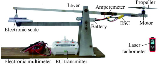
Figure 8: Indoor measurement device for propulsion systems [14].

A series of tests are performed to find the optimal propeller for motor JFRC^® U3508 KV550. In these tests, as shown in Fig. 9, the diameters of the selected APC^® propellers vary from 9 to 13 in, and the results are listed in Table 1. If the propeller is too large (> 12$\times$5.5 in Table 1), then the safety constraint in Eq. (9) is not satisfied because the full-throttle current $I_{\text{e}}^{*}$ exceeds the motor upper limit of $20\text{A}$. If the propeller is too small (< 11$\times$4.5 in Table 1), the full-throttle thrusts $T^{*}$ is too low which leads to an exceedingly small $J_{\text{mep}}$. Therefore, only two propellers (APC 11$\times$5.5 and APC 12$\times$4.5) are close to the optimal solution. Their detailed measurement results are listed in the second and third rows of Table 1.

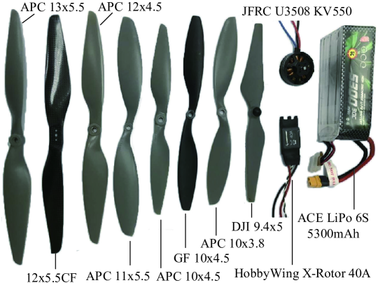
Figure 9: A test case to find the optimal propeller for a motor JFRC U3508.

According to the optimization steps, the maximum values for $T^{*},\eta^{\text{t*}}$, and $m_{\text{mep}}$ obtained from Table 1 are $\overline{T}^{*}=17.84,\overline{\eta}^{\text{t*}}=0.053,$ and $\overline{m}_{\text{mep}}=0.145$. By specifying the weight factors as $\left\{k_{\text{m}1},k_{\text{m}2},k_{\text{m}3}\right\}=\left\{1,1,1\right\}$, the values of $J_{\text{mep}}$ are obtained with the objective function in Eq. (8). The corresponding results are listed in the last column of Table 1. Therefore, the propeller APC 12$\times$4.5 is the optimal propeller for motor JFRC U3508 KV550 according to our method. The obtained optimal propeller and motor combination is in accordance with the recommended result from the JFRC website, which demonstrates the effectiveness of the proposed optimal selection method for propulsion combinations.

Table 1: The results from motor and propeller tests. The propeller name is formed by Diameter $\times$ Pitch (unit: inch).

Propellers	$U_{\text{b}}$(V)	$I_{\text{e}}^{*}$(A)	$T^{*}$(N)	$\eta^{\text{t*}}$	$m_{\text{mep}}$(kg)	$J_{\text{mep}}$
$\leq$ 11$\times$4.5	-	-	< 15	-	-	< 0.7
APC 11$\times$5.5	22.2	15.5	17.84	0.053	0.141	0.85
APC 12$\times$4.5	22.2	19	20.87	0.051	0.145	0.94
$\geq$ 12$\times$5.5	-	> 20	-	-	-	-

In addition to using experimental methods to measure the performance of propulsion combinations, we can use theoretical estimation methods proposed in [14, 15]. The theoretical methods are simpler and more convenient, but their calculation precision is lower than those of the experimental methods, especially when the product parameters provided by the manufacturers are not sufficiently precise. By combining the advantages of both methods, designers can utilize theoretical methods to narrow the search scope, and then use the experimental methods to find the optimal propulsion combination. To make it more convenient for readers to apply the proposed method to multicopter design, a motor-ESC-propeller combination database was published at the website http://rfly.buaa.edu.cn/res16/mepdata.xls. This database includes more than 1500 experimentally verified propulsion combinations, which are adequate for designing multicopters with weights ranging from 0.2 kg to 50 kg.

5.2 Method Implementation and Comparison

To make it simpler and more convenient for common users to assemble their desired multicopters, we developed an online toolbox based on the proposed multicopter design optimization method. This toolbox was published online at

http://flyeval.com/recalc.html

By simply inputting the design requirements, the toolbox outputs the optimal multicopter design including the size, weight, payload capability, and propulsion component selection. The program is fast and can finish within 30 ms by using a web server with a simple configuration (single-core processor and 1 GB of memory). The number of visitors to our online tool exceeded 10,000 in 2018, and feedback indicates that the optimization results from the proposed method are accurate and practical.

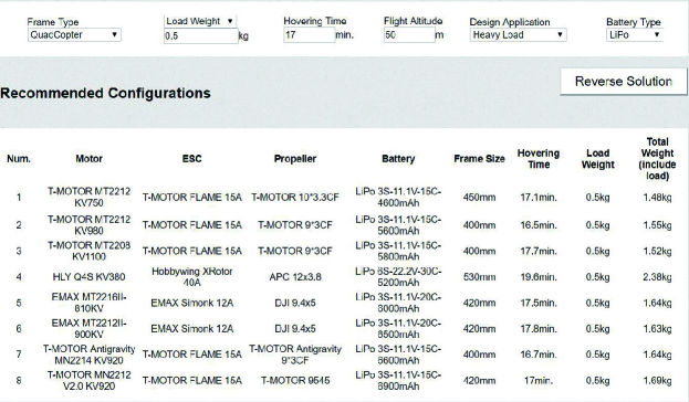
Figure 10: A calculation case from the online design optimization website.

In Fig. 10, an example is presented to design a quadcopter with the following design requirements: payload weight $\hat{m}_{\text{load}}=0.5$ kg, hovering time $\hat{t}_{\text{fly}}=17\text{min}$ and altitude $h=50\text{m}$ (air density $\hat{\rho}=1.22\text{\,kg/m}^{3}$). From our online toolbox, the thrust ratio is obtained as $\hat{\gamma}=0.55$ according to the multicopter usage selection of “heavy load” (see Fig. 10), and the battery power density is $\rho_{\text{b}}$$=240$ W$\cdot$h/kg with the selection of “LiPo battery”. The eight most optimal eight multicopter design results are listed in Fig. 10 and are sorted by the objective function value $J$ in Eq. (27). To verify that the proposed method can obtain multicopter designs in line with expectations, the input design requirements in Fig. 10 are selected based on a popular quadcopter model F450 (airframe diameter: 450mm, weight: 1.5 kg).

It can be observed from Fig. 10 that the diameter and weight of the obtained multicopter design are approximately 450 mm and 1.5 kg, respectively, which are in line with actual design experience. For quantitative verification of the experimental results, a test bench (see Fig. 11) is developed for small-scale multicopters with different design configurations. The comparison verification results for the optimal design obtained in Fig. 10 are listed in Table 2 along with results from the real multicopter on the test bench presented in Fig. 11. Since the performance parameters (e.g., hovering time and payload weight) of a real multicopter are difficult to measure precisely owing to many actual factors (e.g., wind effect, battery states, and controller states), the actual multicopter performance in Table 2 can be considered very close to the optimization results from the website within the measuring errors. The comparison results indicate that the obtained multicopter design is practical for actual multicopter assembly with small estimation errors.

Figure 11: Assembling a real quadcopter with the obtained design optimization results.

Table 2: Experimental verification for the designed results.

Copters	Total weight	Hovering time	Payload Weight	Airframe Size	Battery Capacity
Website	1.48 kg	17.1 min.	0.5 kg	450 mm	4600 mAh
Actual	1.55 kg	18 min.	0.55 kg	450 mm	5000 mAh

In the traditional brutal search method, the computation speed is usually slow because it must traverse all possible multicopter designs and evaluate their performance to find the optimal one. In addition, the performance evaluation will also consume much more time than the proposed method. For example, it takes about 100 ms for the evaluation method in [14] to calculate the performance of each propulsion combination, while our online algorithm needs less than 1 ms. In our simulations, the total computation time of the traditional brutal search method to obtain an optimal multicopter design from a small-scale database (five motors, five propellers, and five ESCs) is up to 12.5 s. In [18, 19], measures were adopted to reduce the computation amount, but at least five seconds was required with a high-performance computer.

Compared with the above methods, the number of traversed multicopter designs and the evaluation time for each design are both significantly reduced in the proposed method. It takes less than 20 ms to obtain a solution from a large-scale database (more than 200 motors) with a low-performance web server. This would take hours and/or days when using the previous optimization design methods.

6 Conclusions and Future Work

This paper proposed a novel and practical method to automatically calculate an optimal multicopter design according to given design requirements. The proposed method obtains the optimal products from a database to form the propulsion system, and subsequently calculates the optimal parameters for the battery and airframe to satisfy the design requirements. Specifically, the entire method involves the use of two algorithms: an offline algorithm and an online algorithm. Because most of the time-intensive computations are completed in the offline algorithm, the proposed method can obtain an optimal multicopter design within 20 ms using a large database (more than 2000 items) with a low-performance web server. This is much faster than previous optimization design methods.

Moreover, practical constraints including safety and compatibility are fully considered during the optimization process such that the obtained design can be directly applied to assemble a real multicopter. Additionally, we proposed a method to map the experimental data from a specific test condition to any other conditions (different altitudes or temperatures), which is crucial for multicopter designers to reduce the testing burden. The experimental results and user feedback for the online toolbox demonstrate the effectiveness and practicability of our method. Along with aerodynamic modeling methods for the body and wing, the method can also be extended to fixed-wing aircraft or other types of aerial vehicles in the future.

Appendices

Appendix A: Modeling of Multicopter Propulsion System

As shown in Fig. 4, the motor voltage $U_{\text{m}}$ (unit: V) and current $I_{\text{m}}$ (unit: A) are controlled by the ESC after receiving the battery voltage $U_{\text{b}}$, the ESC current $I_{\text{e}}$ and the throttle signal $\sigma$. The ESC is an energy conversion module which can be described as

$$U_{\text{m}} =\sigma U_{\text{b}}$$ (30)

$$\eta_{\text{e}} =\frac{I_{\text{m}}U_{\text{m}}}{U_{\text{b}}I_{\text{e}}}$$ (31)

where $\eta_{\text{e}}\in\Theta_{\text{e}}$ is the energy conversion efficiency of the ESC, and $\eta_{\text{e}}=0.93\sim 0.97$ in most cases.

According to [14], the most commonly used multicopter motors are brushless direct-current motors. The mathematical model for a direct-current motor [14, 26] in the steady state (the rotating speed remains constant) is

$$M =K_{\text{T}}\left(I_{\text{m}}-I_{\text{m0}}\right)$$ (32)

$$U_{\text{m}} =I_{\text{m}}R_{\text{m}}+K_{\text{E}}N$$ (33)

where $M$ (unit: N$\cdot$m) and $N$ (unit: RPM) are the torque and rotating speed generated by the motor. Parameters $K_{\text{T}}$ and $K_{\text{E}}$ are motor constants defined as

$$\begin{array}[]{c}\frac{\pi}{30}K_{\text{T}}=K_{\text{E}}=\frac{{{U_{\text{{m0}}}}-{I_{\text{{m0}}}}{R_{\text{{m}}}}}}{{{K_{\text{{V}}}}{U_{\text{{m0}}}}}}\end{array}$$ (34)

where $U_{\text{{m0}}},I_{\text{{m0}}},R_{\text{{m}}},K_{\text{{V}}}\in\Theta_{\text{m}}$ denote the no-load voltage, no-load current, resistance, and KV value which are the basic parameters of a motor.

For multicopters, the most commonly used propellers are fixed-pitch propellers whose output thrust $T$ (unit: N) can be modeled as [27, 28]

$$T =\begin{array}[]{c}C_{\text{T}}\rho\left(\frac{N}{60}\right)^{2}D_{\text{p}}^{4}\end{array}$$ (36)

$$M =\begin{array}[]{c}C_{\text{M}}\rho\left(\frac{N}{60}\right)^{2}D_{\text{p}}^{5}\end{array}$$ (38)

where $C_{\text{T}},C_{\text{M}}\in\Theta_{\text{p}}$ are the thrust coefficient and the torque coefficient of a propeller, $D_{\text{p}}\in\Theta_{\text{p}}$(unit: m) is the propeller diameter, and $\rho$ (unit: kg/$\text{m}^{3}$) is the air density.

Appendix B: Full-throttle Thrust Conversion for Air Density

By combining Eqs. (30)(32)(33)(38) with $\sigma=1$, the motor model in the full-throttle mode is

$$K_{\text{N}}\rho N^{*2}+K_{\text{E}}N^{*}=U_{\text{b}}-I_{\text{m0}}R_{\text{m}}$$ (39)

where $K_{\text{N}}$ is an unknown positive constant parameter. Since both $I_{\text{m0}}$ and $R_{\text{m}}$ are very small values [14], it is reasonable to assume that

$$I_{\text{m0}}R_{\text{m}}\approx 0.$$ (40)

Then, substituting Eqs. (34)(40) into Eq. (39) gives

$$\begin{array}[]{c}K_{\text{N}}\rho N^{*2}+\frac{1}{K_{\text{V}}}N^{*}=U_{\text{b}}\end{array}.$$ (41)

Therefore, the parameter $K_{\text{N}}$ can be obtained according to Eq. (41) with $\rho$ and $N^{*}$ as

$$\begin{array}[]{c}K_{\text{N}}=\frac{K_{\text{V}}U_{\text{b}}-N^{*}}{\rho N^{*2}K_{\text{V}}}\end{array}.$$ (42)

Let $\overline{N}^{*}$ denote the full-throttle rotating speed under air density $\hat{\rho}$, and substitute $\rho=\hat{\rho}$ and $N^{*}=\overline{N}^{*}$ into Eq. (41), the positive solution is given by

$$\begin{array}[]{c}\overline{N}^{*}=\frac{-1+\sqrt{4K_{\text{V}}^{2}K_{\text{N}}U_{\text{b}}\hat{\rho}-1}}{2K_{\text{V}}K_{\text{N}}\hat{\rho}}\end{array}.$$ (43)

Meanwhile, according to Eq. (36), the following proportional expression can be obtained

$$\frac{T^{*}}{\overline{T}^{*}}=\frac{\rho N^{*2}}{\hat{\rho}\overline{N}^{*2}}.$$ (44)

Finally, by substituting parameters $\rho,N^{*},T^{*},K_{\text{V}},U_{\text{b}},\hat{\rho}$ into Eqs. (42)(43)(44) successively, the full-throttle thrust $\overline{T}^{*}$ under air density $\hat{\rho}$ can be obtained as

$$\overline{T}^{*}=\frac{\hat{\rho}\overline{N}^{*2}}{\rho N^{*2}}T^{*}.$$ (45)

Appendix C: Input Current Conversion for Air Density

Combining Eqs. (36)(38) with $T=T_{\text{hover}}$ and $M=M_{\text{hover}}$ gives

$$\frac{T_{\text{hover}}}{M_{\text{hover}}}=\frac{C_{\text{T}}}{C_{\text{M}}}\frac{1}{D_{\text{p}}}.$$ (46)

By substituting Eq. (46) into Eq. (32), the motor hovering current $I_{\text{mHover}}$ is obtained as

$$I_{\text{mHover}}=\frac{M_{\text{hover}}}{K_{\text{T}}}+I_{\text{m0}}=\frac{C_{\text{M}}D_{\text{p}}T_{\text{hover}}}{C_{\text{T}}K_{\text{T}}}+I_{\text{m0}}.$$ (47)

Meanwhile, according to Eq. (36), the propeller hovering speed $N_{\text{hover}}$ can be obtained with parameters $N^{*},T^{*},T_{\text{hover}}$ as

$$N_{\text{hover}}=N^{*}\sqrt{\frac{T_{\text{hover}}}{T^{*}}}.$$ (48)

Similar to Eq. (41), the hovering speed $N_{\text{hover}}$ and the hovering motor voltage $U_{\text{mHover}}$ satisfy the following equation

$$U_{\text{mHover}}=K_{\text{N}}\rho N_{\text{hover}}^{2}+\frac{1}{K_{\text{V}}}N_{\text{hover}}$$ (49)

where $K_{\text{N}}$ is obtained from Eq. (42). Finally, the input hovering current $I_{\text{eHover}}$ is given by

$$I_{\text{eHover}}=\frac{I_{\text{mHover}}U_{\text{mHover}}}{U_{\text{b}}\eta_{\text{e}}}.$$ (50)

According to Eq. (36), the actual propeller rotating speed $\overline{N}_{\text{hover}}$ is determined by parameters $N^{*},T^{*},T_{\text{hover}},\rho,\hat{\rho}$ as

$$\begin{array}[]{c}\overline{N}_{\text{hover}}=N^{*}\sqrt{\frac{\rho T_{\text{hover}}}{\hat{\rho}T^{*}}}\end{array}.$$ (51)

Moreover, according to Eq. (50), one has

$$\frac{I_{\text{eHover}}}{\overline{I}_{\text{eHover}}}=\frac{I_{\text{mHover}}U_{\text{mHover}}}{\overline{I}_{\text{mHover}}\overline{U}_{\text{mHover}}}$$ (52)

where $\overline{U}_{\text{mHover}},\overline{I}_{\text{mHover}}$ are the actual motor voltage and current which can be obtained by Eqs. (47)(49) with $N_{\text{hover}}=\overline{N}_{\text{hover}},\rho=\hat{\rho}$. Finally, the actual input current $\overline{I}_{\text{eHover}}$ under the desired air density $\hat{\rho}$ can be obtained by substituting parameters $\rho,N^{*},T^{*},K_{\text{V}},U_{\text{b}},\hat{\rho},T_{\text{hover}},I_{\text{eHover}}$ into Eqs. (42)(48)(51) as

$$\overline{I}_{\text{eHover}}=\frac{K_{\text{N}}\hat{\rho}\overline{N}_{\text{hover}}^{2}+\frac{1}{K_{\text{V}}}\overline{N}_{\text{hover}}}{K_{\text{N}}\rho N_{\text{hover}}^{2}+\frac{1}{K_{\text{V}}}N_{\text{hover}}}I_{\text{eHover}}.$$ (53)

References

- [1] X. Dai, Q. Quan, J. Ren, and K. Y. Cai, “Iterative learning control and initial value estimation for probe-drogue autonomous aerial refueling of UAVs,” Aerospace Science and Technology, vol. 82-83, pp. 583–593, 2018.
- [2] Q. Quan, Introduction to Multicopter Design and Control. Springer, Singapore, 2017.
- [3] Y. Ke, K. Wang, and B. M. Chen, “Design and implementation of a hybrid UAV with model-based flight capabilities,” IEEE/ASME Transactions on Mechatronics, vol. 23, no. 3, pp. 1114–1125, 2018.
- [4] D. Santamaría, F. Alarcón, A. Jiménez, A. Viguria, M. Béjar, and A. Ollero, “Model-based design, development and validation for UAS critical software,” Journal of Intelligent & Robotic Systems, vol. 65, no. 1-4, pp. 103–114, 2012.
- [5] T. Oktay, M. Konar, M. Onay, M. Aydin, and M. A. Mohamed, “Simultaneous small UAV and autopilot system design,” Aircraft Engineering and Aerospace Technology, vol. 88, no. 6, pp. 818–834, 2016.
- [6] C. E. Riboldi, “An optimal approach to the preliminary design of small hybrid-electric aircraft,” Aerospace Science and Technology, vol. 81, pp. 14–31, 2018.
- [7] S. Zhang, H. Li, and A. A. Abbasi, “Design methodology using characteristic parameters control for low reynolds number airfoils,” Aerospace Science and Technology, vol. 86, pp. 143–152, 2019.
- [8] H. Yeo, “Design and aeromechanics investigation of compound helicopters,” Aerospace Science and Technology, vol. 88, pp. 158–173, 2019.
- [9] Y. Volkan Pehlivanoglu, “Efficient accelerators for PSO in an inverse design of multi-element airfoils,” Aerospace Science and Technology, vol. 91, pp. 110–121, 2019.
- [10] N. A. Vu, D. K. Dang, and T. Le Dinh, “Electric propulsion system sizing methodology for an agriculture multicopter,” Aerospace Science and Technology, vol. 90, pp. 314–326, 2019.
- [11] H. Youngren and M. Chang, “Test, analysis and design of propeller propulsion systems for MAVs,” in 49th AIAA Aerosp. Sci. Meeting New Horizons Forum Aerosp. Expo. AIAA 2011-876, Jan. 2011.
- [12] R. W. Deters, G. K. Ananda, and M. S. Selig, “Reynolds number effects on the performance of small-scale propellers,” in 32nd AIAA Applied Aerodynamics Conference. AIAA 2007-2151, 2014, pp. 1–43.
- [13] C. M. Burt, X. Piao, F. Gaudi, B. Busch, and N. Taufik, “Electric motor efficiency under variable frequencies and loads,” Journal of irrigation and drainage engineering, vol. 134, no. 2, pp. 129–136, 2008.
- [14] D. Shi, X. Dai, X. Zhang, and Q. Quan, “A practical performance evaluation method for electric multicopters,” IEEE/ASME Transactions on Mechatronics, vol. 22, no. 3, pp. 1337–1348, 2017.
- [15] X. Dai, Q. Quan, J. Ren, and K.-Y. Cai, “An Analytical Design Optimization Method for Electric Propulsion Systems of Multicopter UAVs with Desired Hovering Endurance,” IEEE/ASME Transactions on Mechatronics, vol. 24, no. 1, pp. 228–239, 2019.
- [16] X. Dai, Q. Quan, J. Ren, and C. Kai-Yuan, “Efficiency optimization and component selection for propulsion systems of electric multicopters,” IEEE Transactions on Industrial Electronics, vol. 66, no. 10, pp. 7800–7809, 2019.
- [17] Ø. Magnussen, G. Hovland, and M. Ottestad, “Multicopter UAV design optimization,” in 2014 IEEE/ASME 10th International Conference on Mechatronic and Embedded Systems and Applications (MESA), sep. 2014, pp. 1–6.
- [18] Ø. Magnussen, M. Ottestad, and G. Hovland, “Multicopter design optimization and validation,” Modeling, Identification and Control, vol. 36, no. 2, pp. 67–79, 2015.
- [19] V. Arellano-Quintana, E. Portilla-Flores, E. Merchan-Cruz, and P. Nino-Suarez, “Multirotor design optimization using a genetic algorithm,” in Unmanned Aircraft Systems (ICUAS), 2016 International Conference on. IEEE, 2016, pp. 1313–1318.
- [20] F. Tian and M. Voskuijl, “Mechatronic design and optimization using knowledge-based engineering applied to an inherently unstable and unmanned aerial vehicle,” IEEE/ASME Transactions on Mechatronics, vol. 21, no. 1, pp. 542–554, 2016.
- [21] M. Orsag and S. Bogdan, “Influence of forward and descent flight on quadrotor dynamics,” in Recent Advances in Aircraft Technology. InTech, 2012.
- [22] M. Cavcar, “The international standard atmosphere (ISA),” Anadolu University, Turkey, vol. 30, p. 9, 2000.
- [23] M. Wu, “T-motor official website,” http://store-en.tmotor.com/, accessed September 28, 2018.
- [24] D. Bershadsky, S. Haviland, and E. N. Johnson, “Electric multirotor UAV propulsion system sizing for performance prediction and design optimization,” in 57th AIAA/ASCE/AHS/ASC Structures, Structural Dynamics, and Materials Conference. AIAA 2016-0581, Jan. 2015.
- [25] A. M. Harrington, “Optimal propulsion system design for a micro quad rotor,” Master’s thesis, University of Maryland, College Park, 2011.
- [26] S. Chapman, Electric machinery fundamentals. Tata McGraw-Hill Education, 2005.
- [27] M. Merchant and L. S. Miller, “Propeller performance measurement for low Reynolds number UAV applications,” in 44th AIAA Aerospace Sciences Meeting and Exhibit. AIAA 2006-1127, Jan. 2006.
- [28] R. S. Merrill, “Nonlinear aerodynamic corrections to blade element momentum modul with validation experiments,” Utah State University, Tech. Rep. Paper 67, 2011.