Homogeneous Analysis of Hot Earths: Masses, Sizes, and Compositions

Abstract

Terrestrial planets have been found orbiting Sun-like stars with extremely short periods — some as short as 4 hours. These “ultra-short-period planets” or ”hot Earths” are so strongly irradiated that any initial H/He atmosphere has probably been lost to photoevaporation. As such, the sample of hot Earths may give us a glimpse at the rocky cores that are often enshrouded by thick H/He envelopes on wider-orbiting planets. However, the mass and radius measurements of hot Earths have been derived from a hodgepodge of different modeling approaches, and include several cases of contradictory results. Here, we perform a homogeneous analysis of the complete sample of 11 known hot Earths with an insolation exceeding 650 times that of the Earth. We combine all available data for each planet, incorporate parallax information from Gaia to improve the stellar and planetary parameters, and use Gaussian Process regression to account for correlated noise in the radial-velocity data. The homogeneous analysis leads to a smaller dispersion in the apparent composition of hot Earths, although there does still appear to be some intrinsic dispersion. Most of the planets are consistent with an Earth-like composition (35% iron and 65% rock), but two planets (K2-141b and K2-229b) show evidence for a higher iron fraction, and one planet (55 Cnc e) has either a very low iron fraction or an envelope of low-density volatiles. All of the planets are less massive than 8 $M_{\oplus}$, despite the selection bias towards more massive planets, suggesting that 8 $M_{\oplus}$ is the critical mass for runaway accretion.

1 Introduction

Planets with orbital periods shorter than 1 day are known as “ultra-short-period” (USP) planets (Winn et al., 2018). They occur around $\approx$0.5% of Sun-like stars, and their radii rarely exceed 2 $R_{\oplus}$ (Sanchis-Ojeda et al., 2014). Prime examples include CoRoT-7b (Léger et al., 2009) and Kepler-78b (Sanchis-Ojeda et al., 2013). The orbits of USP planets are so small that they are often within the dust sublimation radius ($a/R_{\star}\sim 8$ for Sun-like stars, Isella et al., 2006), where the formation of Earth-mass cores was probably impossible. This makes the formation of USP planets an interesting problem, similar to the longstanding problem of the formation of hot Jupiters. In fact, an early idea was that USP planets are the cores of hot Jupiters which lost their gaseous envelopes due to tidal disruption or atmospheric erosion (see, e.g., Valsecchi et al., 2015). This idea is now disfavored both because of the limited atmospheric erosion rate (e.g. Lammer et al., 2009) and the fact that the host stars of hot Jupiters and USP planets have different metallicity distributions (Winn et al., 2017). Instead, the USP planets seem to be more closely related to the more abundant population of planets discovered by the Kepler mission, with sizes ranging up to 4 $R_{\oplus}$ and orbital periods shorter than a few months (Sanchis-Ojeda et al., 2014; Lee & Chiang, 2017; Petigura et al., 2018).

The radius distribution of these Kepler planets is bimodal, with a dip in occurrence for planets with sizes between 1.5 and 2.0 $R_{\oplus}$ (Fulton et al., 2017). This feature had been predicted, based on theories of the photoevaporation of H/He planetary atmospheres (Owen & Wu, 2017). In the same theories, photoevaporation should have gone to completion for USP planets, removing any H/He envelope and exposing the rocky core. Supporting this picture is the fact that almost all USP planets have sizes below 2 $R_{\oplus}$, on the small end of the bimodal radius distribution. In the alternative explanation of Zeng et al. (2019) that attributed the bimodal radius distribution to a rock-ice transition, the USP planets are also exposed rocky worlds. Thus, by studying USP planets, we may be learning about the rocky cores that lie inside the lower-density planets with sizes between 2 and 4 $R_{\oplus}$. Moreover, the extremely short periods of USP planets facilitate the measurement of their masses through the Doppler technique. This is because the velocity amplitude varies as $P^{-1/3}$ and because there is usually a clean separation between the short orbital period and the longer timescale of stellar rotation (one of the timescales over which stellar activity leads to spurious Doppler signals).

In this Letter, we present a homogeneous analysis of the masses, sizes, and compositions of a sample of strongly irradiated planets, hoping to illuminate the origin and evolution of these planets through knowledge of their possible range of compositions. Are they stripped of H/He atmospheres, as photoevaporation theory would require? Did they migrate from beyond the snow line, in which case a large complement of water or other volatile elements might still be present? Were their rocky mantles stripped by giant impacts, leading to an enhancement in the iron fraction similar to that of Mercury (Benz et al., 2008)?

We felt a homogeneous analysis was warranted because the results in the literature were reported by different groups using different procedures to determine the stellar parameters and to mitigate the effects of time-correlated noise in the radial-velocity data. For example, K2-106b was reported by Guenther et al. (2017) to have an iron mass fraction of $80^{+20}_{-30}\%$, while Sinukoff et al. (2017) concluded that the composition was compatible with that of the Earth (35% iron). For this work, we combined all the previously published datasets, used the parallaxes from Gaia Data Release 2 (Gaia Collaboration et al., 2018) to refine the stellar parameters, and employed a Gaussian Process framework (Dai et al., 2017) to disentangle planetary radial velocity signals from correlated noise. Previous works (e.g. Southworth, 2008, 2009) have demonstrated the value of a homogeneous analysis when comparing the properties of exoplanetary systems reported by different groups.

2 Sample Selection

The criterion $P_{\rm orb}$<1 day for USP planets is convenient, but a quantity more directly relevant to our questions is the bolometric flux $F_{\rm p}$ delivered to the planet from the star. Our sample was defined by the requirement $F_{\rm p}/F_{\oplus}>650$, where the somewhat arbitrary number 650 was taken from the study of the radius/flux distribution by Lundkvist et al. (2016). We selected “hot Earths” by requiring $R_{\rm p}/R_{\oplus}<2$. This radius cut filtered out hot Jupiters as well as the extraordinary “hot Neptune” NGTS-4b, with $M_{\rm p}/M_{\oplus}=20.6\pm 3.0$, $R_{\rm p}/R_{\oplus}=3.18\pm 0.26$, and $F/F_{\oplus}\approx 950$ (West et al., 2018). We also restricted attention to FGK dwarf stars by restricting $\log g>4$. Table 1 summarizes the characteristics of the 11 hot Earths in our sample.

3 Stellar Parameters

To determine the stellar parameters, we used the same procedures as Dai et al. (2018), described below. We had previously validated these procedures using a sample of stars for which the radius and mass have also been determined precisely using asteroseismology. The input information was the parallax from Gaia Data Release 2 (Gaia Collaboration et al., 2018); the observed spectroscopic parameters $T_{\rm eff}$, $\log g$, and [Fe/H]; the $K$-band apparent magnitude; and stellar evolutionary models computed with Modules for Experiments in Stellar Astrophysics (MESA; Paxton et al., 2011).

The $K$-magnitudes were taken from the Two Micron All Sky Survey (2MASS; Skrutskie et al., 2006). We corrected for extinction $A_{K}$ using the value of $E(B-V)$ and extinction vectors from the dust map Bayestar17 (Green et al., 2018). We adopted a $30\%$ fractional uncertainty for $A_{K}$, following Fulton & Petigura (2018). We adopted the distance estimates from Bailer-Jones et al. (2018) instead of using the parallaxes directly, although the difference was minor for our sample stars, which are within a few hundred parsecs. We adopted spectroscopic parameters reported in the literature (Table 1). We inflated the uncertainties on uncertainties of $T_{\rm eff}$ to 110 K, $\log g$ to 0.1, and [Fe/H] to 0.1 to reflect the systematic offsets that may exist between the different methods used to infer the spectroscopic parameters. We then sampled the MESA Isochrones & Stellar Tracks (Dotter, 2016) with the priors on the spectroscopic parameters, the $K$-band magnitude, the extinctions and the Gaia distance using the isochrones package by Morton (2015). This Bayesian analysis yielded posterior distribution of the stellar mass, radius and the stellar mean densities. Table 1 reports the results.

4 Transit Analysis

For the Kepler systems in our sample, we used the Pre-search Data Conditioning light curves available on the Mikulski Archive for Space Telescopes website. For the K2 systems, we downloaded the target pixel files and produced the light curves using the procedure described by Dai et al. (2017). We used short-cadence light curve whenever possible. For 55 Cnc, we used the HST/STIS light curve presented by Bourrier et al. (2018). For CoRoT-7, we downloaded the light curves from the CoRoT N2 public archive .

Using from the transit ephemerides reported in the literature (Table 1), we isolated the transit data. Only the data obtained within one full transit duration of the transit midpoint were retained; hence, the total timespan of each transit segment was two full transit durations. We inspected the data from each transit segment visually, to remove obviously bad data points. We fitted the light curves using the Batman package (Kreidberg, 2015). We assumed the limb darkening law to be quadratic and placed Gaussian priors on the coefficients with widths of 0.3 and central values based upon theoretical stellar atmosphere models computed with EXOFAST (Eastman et al., 2013). The other transit parameters included the orbital period $P_{\rm orb}$, the midtransit time ($T_{\rm c}$), the planet-to-star radius ratio ($R_{\rm p}/R_{\star}$), the scaled orbital distance ($a/R_{\star}$), and the cosine of the orbital inclination ($\cos I$) for each transiting planets in the system. For systems with only long-cadence (29.4 min) data, we computed the theoretical transit model 30 times at 1-min interval. We then averaged the 30 flux values before comparing it with the observed flux level to mimic the effect of finite integration time.

We created a phase-folded transit light curve for subsequent analysis. Two of the systems display detectable transit-timing variations (TTV): WASP-47 and Kepler-10 (Becker et al., 2015; Ofir et al., 2018). For those systems, we inserted an additional step. We began by fitting a constant-period transit model using all the available data. Then, we used the best-fitting model as a template to derive individual transit times. The phase-folded light curve was created based on the model including TTVs.

We fitted simultaneously for the parameters of all the transiting planets in each system. We imposed a Gaussian prior on the stellar mean density (Section 2), a log-uniform prior on $R_{\rm p}/R_{\star}$, and a uniform prior on $\cos I>0$. We assumed the orbit of the hot Earth to be circular, based on the theoretical expectation that the tidal circularization timescale is on the order of 10 Myr (Winn et al., 2018). The outer planets were allowed to have eccentric orbits. For more efficient sampling, we did not use the eccentricity $e$ and the argument of pericenter $\omega$ as parameters; instead, we used $\sqrt{e}\cos\omega$ and $\sqrt{e}\sin\omega$ which have a lower covariance. We sampled the posterior distribution using the Markov Chain Monte Carlo technique implemented in the emcee code (Foreman-Mackey et al., 2013). Table 2 reports the results for the key parameter $R_{\rm p}/R_{\star}$.

5 Radial Velocity Analysis

We compiled all available radial velocity data sets for each planet (see Table 2). For WASP-47, we removed from consideration the 29 data points that were based on spectra obtained during transit, because we did not want to model the Rossiter-McLaughlin effect. We modeled the radial velocity measurements in a Gaussian Process framework similar to that described by Dai et al. (2017). In brief, we adopted a quasi-periodic kernel:

$$C_{ij}=h^{2}\exp{\left[-\frac{(\Delta t_{ij})^{2}}{2\tau^{2}}-\Gamma\sin^{2}{\frac{\pi\Delta t_{ij}}{T}}\right]}+\left[\sigma_{i}^{2}+\sigma_{\text{jit}}^{2}\right]\delta_{ij}$$ (1)

where $C_{ij}$ is the covariance matrix, $\delta_{ij}$ is the Kronecker delta, $\sigma_{\rm jit}$ is the “stellar jitter” (any noise component beyond the measurement uncertainty that is uncorrelated in time), $h$ is the covariance amplitude, $t_{i}$ is the time of individual observation, $\Delta t_{ij}=t_{i}-t_{j}$, $\tau$ is the correlation timescale, $T$ is the period of the covariance, and $\Gamma$ dictates the relative importance of the Gaussian and periodic components of the kernel. We set the priors for the “hyperparameters” of this kernel ($\tau$, $\Gamma$, and $T$) by analyzing the out-of-transit flux variation in the light curves. The underlying idea is that the both the flux variations and the spurious Doppler shifts originate from surface inhomogeneities of the host star, but the light curve has a higher precision and better time sampling than the radial-velocity data.

After fitting the light curves with a Gaussian process, we used the posteriors for the hyperparameters as priors in the radial-velocity analysis. The adopted likelihood function has the following form:

$$\log{\mathcal{L}}=-\frac{N}{2}\log{2\pi}-\frac{1}{2}\log{|\bf{C}|}-\frac{1}{2}\bf{r}^{\text{T}}\bf{C}^{-\text{1}}\bf{r}$$ (2)

where $N$ is the number of data points, $\bf{C}$ is the covariance matrix, and $\bf{r}$ is the difference between the observed radial velocity and the calculated Keplerian radial velocity. Again, we assumed that the hot Earths have circular orbits, and allowed for nonzero eccentricity of the outer orbits. We imposed Gaussian priors on $P_{\text{orb}}$ and $T_{\text{c}}$ for the transiting planets based on the analysis of Section 4. We imposed log-uniform priors on the RV semiamplitudes $K$, the covariance amplitude $h$, and the jitter parameters. We imposed uniform priors on the RV offset of each spectrograph, $\sqrt{e}\cos\omega$ ($[-1,1]$) and $\sqrt{e}\sin\omega$ ($[-1,1]$). Again, we sampled the posterior distribution using emcee (Foreman-Mackey et al., 2013).

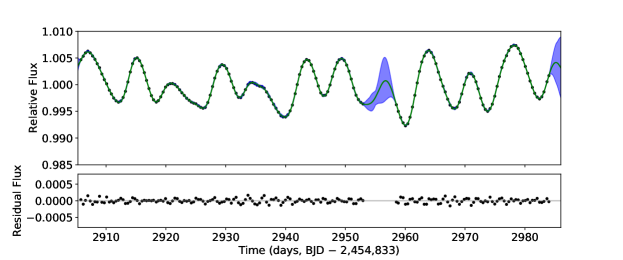
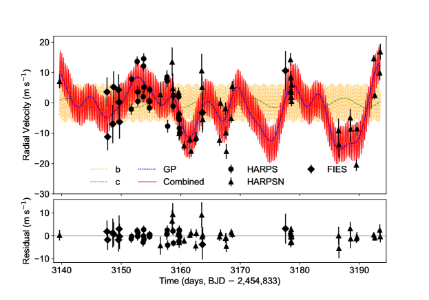
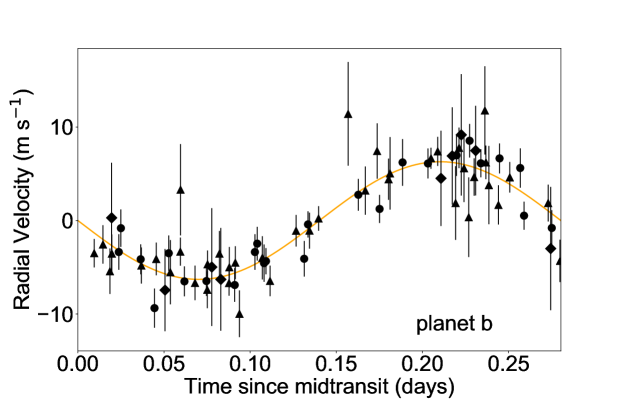
Figure 1: Illustrative example of our Gaussian Process radial-velocity analysis, for the K2-141 system. Top: The out-of-transit flux variation is used to train the hyperparameters of the Gaussian Process model. Middle: Measured and calculated radial velocities of planets b and c. Bottom: Data and best-fitting model for planet b, after subtracting the calculated radial-velocity variation due to planet c and stellar activity.

Table 2 gives the resulting mass determinations for the hot Earths. Figure 1 shows the radial-velocity results for the representative system K2-141.

6 Discussion

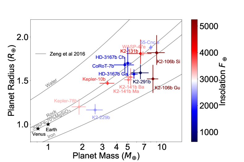
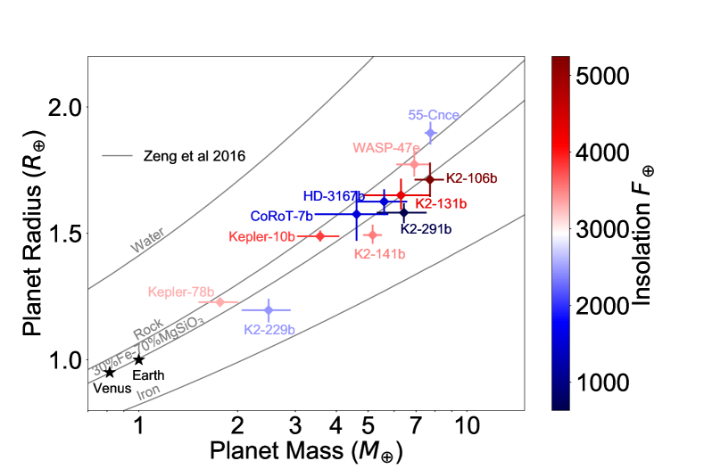
Figure 2: Masses and radii of hot Earths in our sample ($R_{\rm p}/R)_{\oplus}<2$, $F/F_{\oplus}>650$, $\log g$ > 4.0) and theoretical mass-radius curves for various compositions from Zeng et al. (2016). The color of the symbols conveys the value of $F/F_{\oplus}$. Top: Results drawn from the literature. For the cases in which more than one report is available, the leading initials of the first author are printed (see Table 2). Bottom: Results from our analysis. In general, the uncertainties are lower, and the dispersion in the implied composition is smaller.

Figure 2 compares the results of our uniform analysis to those reported in the literature. The overall impression is that we found a smaller dispersion in the implied compositions of the hot Earths. We were also able to achieve more precise results in some cases. This is partly thanks to the parallax information provided by Gaia, which led to substantial reduction in the planetary radius uncertainty for systems that had been analyzed prior to Gaia Data Release 2. For example, Kepler-78b was reported to have $R_{p}=1.20\pm 0.09R_{\oplus}$ by Howard et al. (2013), while we found $R_{p}=1.228^{+0.018}_{-0.019}R_{\oplus}$. In other cases, improvement was achieved by combining RV datasets from different groups, and by using Gaussian Process regression.

To quantify the constraints on composition, we used a simple two-layer model, in which each planet is assumed to have an iron core and a rocky (MgSiO₃) mantle, using the procedure described by Zeng et al. (2016). Table 2 gives the resulting constraints on the iron mass fraction. One noteworthy result is that K2-106b does not appear to be as iron-rich as had been previously thought (Guenther et al., 2017). Instead of 80%, our analysis gave an iron fraction of 40$\pm 23$%, which resembles the results for the other hot Earths.

6.1 Are USPs really rocky?

All in all, our uniform analysis not only tightened the constraints on the mass and radius of individual planets, but also led to a smaller dispersion of iron fractions centered on an Earth-like composition. The mean core mass fraction is $26\%$ and the standard deviation is 23%. In a few cases, the posterior for the iron mass fraction extends to negative values; such cases should be interpreted as an indication that the planet is probably composed of lower-density material (volatiles) in addition to rock and iron.

We tested to see whether the core mass fraction of the planets is correlated with any of the stellar or planetary parameters, including bolometric insolation, orbital period, planetary mass, planetary radius and host star metallicity. None of these parameters showed a statistically significant correlation with the core mass fraction ($p<5$%). In particular, the lack of correlation with bolometric insolation can be interpreted as additional evidence that hot Earths are free of H/He envelopes, as photoevaporation theory would predict. If the planet’s mass budget had even a few percent of H/He, there would likely be a reduction in radius with increasing irradiation (Lopez, 2017) similar to the pattern that is seen for mini-Neptunes (2 to 4 $R_{\oplus}$) just outside of the “hot Neptune desert” (Fulton & Petigura, 2018). Mini-Neptunes have systematically smaller radii when the bolometric flux is high.

Although an atmosphere of hydrogen and helium probably cannot survive on a hot Earth, what about an atmosphere with a higher mean molecular weight, composed of water, carbon dioxide, or other volatiles? Simulations by Lopez (2017) suggest that volatile atmospheres can survive on hot Earths over geological timescales. Any hot Earths with substantial volatile atmospheres might show up in between the “rock” and “water” lines in Figure 2. However, we found no cases in which a substantial volatile atmosphere is required to explain the data. To quantify this result, we assumed that these planets have Earth-like cores of Fe-MgSiO₃ ratio of 3:7 on top of which is a variable amount of water envelope. Table 2 gives the $2-\sigma$ upper limits on the water mass fraction. The individual upper limits generally favors a water content less than 10 or 20% by mass. In this sense, the hot Earths are consistent with a formation scenario in which the planetesimals were volatile-depleted, i.e., within the snowline.

The two planets that appear to depart most from an Earth-like composition (although with modest statistical significance) are WASP-47 e and 55 Cnc e. Vanderburg et al. (2017) also highlighted these two systems as peculiar. They are the only systems known that have both USP planets and close-in giant planets (in 4 and 15-day orbits, respectively). The host stars are also the most metal-rich among the sample, with [Fe/H] of 0.3 and 0.4. Combined with their lower planetary densities, these may be clues that the hot Earths formed in a different way around WASP-47 and 55 Cnc. They might be cases of disk migration from beyond the snowline. This would explain the presence of gas giants, since it is easier to achieved runaway gas accretion beyond the snowline, and it would also explain why WASP-47 e and 55 Cnc e may have volatile atmospheres. It is worth noting WASP-47 e and 55 Cnc e are the largest hot Earths (by radius) in our sample. Both have $R_{\rm p}>1.6\,R_{\oplus}$, the approximate value of the critical radius separating rocky and volatile-enhanced planets within the larger sample of sub-Neptune planets (Rogers, 2015). Furthermore, Angelo & Hu (2017) have argued that 55 Cnc e must possess some form of thick atmosphere to explain the high heat redistribution efficiency that is indicated in phase-curve observations (Demory et al., 2016). Alternatively Dorn et al. (2019) proposed that these two planets are iron-poor and low in density because they are rich in calcium and aluminum whcih condensed earlier within the protoplanetary disk.

6.2 Threshold mass for runaway accretion

As mentioned in the Introduction, there are several indications that hot Earths are not a later evolutionary state of hot Jupiters, but rather are drawn from the same basic population as the more abundant and longer-period sub-Neptune planets. This conclusion is also supported on more theoretical grounds. Ginzburg & Sari (2017) studied the fate of Roche-Lobe-overflowing (RLO) hot Jupiters. They found that, depending on the planet’s core mass, a RLO hot Jupiter either gets entire swallowed by the host star or leave behind a remnant planet with a thick atmosphere. Neither scenario would produce the observed sample of rocky hot Earths. The rate of hydrodynamic mass loss (including photoevaporation) is strongly dependent on planet mass: while the H/He envelope of a $5\,M_{\oplus}$ planet can be easily dissipated over 100 Myr, the timescale can be longer than a Hubble time for planets more massive than Neptune (e.g. Wang & Dai, 2017). Hence, photoevaporation is unable to strip a hot Jupiter down to a hot Earth.

Thus, it seems possible or even probable that when we observe a hot Earth, we are really looking at the exposed rocky core of a sub-Neptune. If so, then the hot Earths are a sample of rocky cores that managed to avoid runaway gas accretion and promotion into a giant planet. With these premises, we can use the maximum observed mass of a hot Earth as an indicator of the critical mass for initiating runaway gas accretion. We note that the selection bias of radial-velocity mass measurements towards higher-mass planets works in our favor, since we are interested establishing the maximum mass.

The critical mass for runaway gas accretion has been studied for decades. Assuming a radiative envelope, the critical mass has only a logarithmic dependence on the local disk properties, and is often taken to be $10\,M_{\oplus}$ (e.g. Rafikov, 2006). More recently, Lee & Chiang (2016) advocated for the importance of envelope opacity and revised the threshold mass to be between 2 and $8\,M_{\oplus}$. Our uniform analysis of hot Earths seems to favor an upper limit of about $8\,M_{\oplus}$. This assumes that the planetary masses have not been significantly reduced by giant impact collisions, an issue we will visit in the next section.

6.3 Mercury formation scenario

Mercury has an iron mass fraction of about 70%, which is significantly larger than any of the other planets in the solar system (Hauck II et al., 2013). Another explanation is a giant impact collision that removed much of the planet’s rocky mantle (Benz et al., 2008). Bonomo et al. (2019) also invoked a giant impact scenario to explain why Kepler-107c attained a much higher mean density than the similarly-sized innermost planet b. Alternatively, Lewis (1972) attributed the iron enhancement of Mercury to the high temperatures that prevail near the Sun, which favor iron condensation. More recently, Wurm et al. (2013) called attention to the process of photophoresis that separates grains of different thermal conductivity and creates a compositional gradient in the disk.

In all of these scenarios, one might expect hot Earths to be just as iron-enriched as Mercury, or even more so. The orbital velocity of a hot Earth is much larger, leading to more disruptive giant impact collisions. The much hotter conditions of hot Earths should also make the effect of condensation temperature and photophoresis more pronounced. Our results suggest that although a few hot Earths do show evidence for iron enhancement (K2-141b and K2-229b), a Mercury-like composition is not the norm. Could this mean that an Earth-like composition is universal for all rocky worlds (Dressing et al., 2015)? Could it also mean that the conditions for removing mantle material through giant impacts are relatively rare?

Enlarging the sample of hot Earths — especially those with host stars bright enough for mass measurements — is a high priority for future work. The ongoing NASA Transiting Exoplanet Survey Satellite (TESS) mission (Ricker et al., 2014) will help in this regard. This nearly all-sky transit survey should allow the sample of hot Earths to be doubled. More importantly, the host stars will be systematically brighter than the typical stars in the Kepler and K2 surveys. TESS will also survey stars over a broader range of spectral types. In combination with the suite of new Doppler spectrographs coming online, the larger and more diverse sample will hopefully improve our understanding of these extreme worlds.

Table 1: Stellar Parameters

System	$T_{\rm eff}$   (K)	log $g$	[Fe/H]	Spectroscopic Source	$M_{\star}$ ($M_{\odot}$)	$R_{\star}$ ($R_{\odot}$)	$\rho_{\star}$ (g cm-3)
55 Cnc e	5172$\pm$18	4.43$\pm$0.02	0.35$\pm$0.10	Yee et al. (2017)	0.873${}^{+0.051}_{-0.035}$	0.954${}^{+0.017}_{-0.018}$	1.41${}^{+0.15}_{-0.10}$
CoRot-7b	5313$\pm$73	4.54$\pm$0.04	0.03$\pm$0.07	Torres et al. (2012)	0.884${}^{+0.029}_{-0.032}$	0.8389${}^{+0.0093}_{-0.0088}$	2.11${}^{+0.17}_{-0.19}$
GJ 9827b	4255$\pm$110	4.70$\pm$0.15	-0.28$\pm$0.12	Niraula et al. (2017)	0.606${}^{+0.020}_{-0.015}$	0.5994${}^{+0.0081}_{-0.0085}$	3.97${}^{+0.20}_{-0.15}$
HD 3167b	5261$\pm$60	4.47$\pm$0.05	0.04$\pm$0.05	Christiansen et al. (2017)	0.837${}^{+0.053}_{-0.043}$	0.880${}^{+0.012}_{-0.013}$	1.73${}^{+0.18}_{-0.14}$
K2-106b	5496$\pm$46	4.42$\pm$0.05	0.06$\pm$0.03	Sinukoff et al. (2017)	0.902${}^{+0.057}_{-0.046}$	0.981${}^{+0.019}_{-0.018}$	1.35${}^{+0.14}_{-0.12}$
K2-131b	5200$\pm$100	4.62$\pm$0.10	-0.02$\pm$0.08	Dai et al. (2017)	0.793${}^{+0.024}_{-0.040}$	0.744${}^{+0.010}_{-0.009}$	2.71${}^{+0.14}_{-0.19}$
K2-141b	4599$\pm$79	4.62${}^{+0.02}_{-0.03}$	-0.06${}^{+0.08}_{-0.10}$	Malavolta et al. (2018)	0.706${}^{+0.021}_{-0.015}$	0.6862${}^{+0.0066}_{-0.0080}$	3.86${}^{+0.16}_{-0.18}$
K2-229b	5185$\pm$32	4.56${}^{+0.03}_{-0.05}$	-0.06$\pm$0.02	Santerne et al. (2018)	0.804 ${}^{+0.038}_{-0.048}$	0.781${}^{+0.012}_{-0.012}$	2.38${}^{+0.18}_{-0.20}$
K2-291b	5520$\pm$60	4.50$\pm$0.05	0.08$\pm$0.04	Kosiarek et al. (2019)	0.926 ${}^{+0.046}_{-0.048}$	0.904${}^{+0.012}_{-0.012}$	1.77${}^{+0.13}_{-0.14}$
Kepler-10b	5708$\pm$28	4.344$\pm$0.004	-0.15$\pm$0.04	Dumusque et al. (2014)	0.905${}^{+0.050}_{-0.044}$	1.075${}^{+0.016}_{-0.015}$	1.029${}^{+0.090}_{-0.084}$
Kepler-78b	5121$\pm$44	4.61$\pm$0.06	-0.08$\pm$0.04	Howard et al. (2013)	0.779${}^{+0.032}_{-0.046}$	0.7475${}^{+0.0077}_{-0.0078}$	2.63${}^{+0.16}_{-0.19}$
WASP-47e	5552$\pm$75	4.34$\pm$0.03	0.38$\pm$0.05	Vanderburg et al. (2017)	1.008${}^{+0.053}_{-0.047}$	1.125${}^{+0.027}_{-0.026}$	1.00${}^{+0.10}_{-0.09}$

=2.3in

Table 2: Planetary Parameters

System	$P_{\rm orb}$(days)	$K$(m s-1)	$R_{p}/R_{\star}$	$M_{p}$ ($M_{\oplus}$)	$R_{p}$ ($R_{\oplus}$)	$\rho_{p}$ (g cm-3)	Core Mass Fraction1	Water Content2	Radial Velocity Source
55 Cnc e	0.737	6.00${}^{+0.17}_{-0.17}$	0.01821${}^{+0.00027}_{-0.00029}$	7.74${}^{+0.37}_{-0.30}$	1.897${}^{+0.044}_{-0.046}$	6.25${}^{+0.74}_{-0.70}$	-0.10$\pm$0.14	$<0.28$	Bourrier et al. (2018)
CoRoT-7b	0.854	3.37${}^{+0.84}_{-0.86}$	0.0172${}^{+0.0010}_{-0.0011}$	4.6${}^{+1.1}_{-1.2}$	1.58${}^{+0.10}_{-0.10}$	6.5${}^{+2.8}_{-3.0}$	0.11$\pm$0.45	<0.36	Haywood et al. (2014)
GJ-9827b	1.209	4.10${}^{+0.35}_{-0.34}$	0.02401${}^{+0.00038}_{-0.00049}$	4.89${}^{+0.43}_{-0.42}$	1.571${}^{+0.033}_{-0.039}$	6.9${}^{+1.0}_{-1.1}$	0.22$\pm$0.15	<0.12	Teske et al. (2018); Rice et al. (2019)
									Prieto-Arranz et al. (2018)
HD-3167b	0.960	4.08${}^{+0.70}_{-0.69}$	0.01692${}^{+0.00045}_{-0.00050}$	5.59${}^{+0.98}_{-0.96}$	1.626${}^{+0.048}_{-0.054}$	7.2$\pm$1.9	0.23$\pm$0.27	<0.16	Christiansen et al. (2017); Gandolfi et al. (2017)
K2-106b	0.571	6.37${}^{+0.60}_{-0.62}$	0.01598${}^{+0.00056}_{-0.00057}$	7.72${}^{+0.80}_{-0.79}$	1.712${}^{+0.068}_{-0.068}$	8.5$\pm$1.9	0.40$\pm$0.23	<0.17	Sinukoff et al. (2017); Guenther et al. (2017)
K2-131b	0.369	6.55${}^{+1.48}_{-1.48}$	0.02032${}^{+0.00076}_{-0.00064}$	6.3${}^{+1.4}_{-1.4}$	1.651${}^{+0.065}_{-0.056}$	7.7${}^{+2.7}_{-2.6}$	0.31$\pm$0.34	<0.16	Dai et al. (2017)
K2-141b	0.280	6.36${}^{+0.41}_{-0.40}$	0.01993${}^{+0.00052}_{-0.00042}$	5.16${}^{+0.35}_{-0.34}$	1.493${}^{+0.041}_{-0.035}$	8.5${}^{+1.3}_{-1.2}$	0.53$\pm$0.15	<0.02	Malavolta et al. (2018); Barragán et al. (2018)
K2-229b	0.584	2.20${}^{+0.36}_{-0.37}$	0.01403${}^{+0.00048}_{-0.00052}$	2.49${}^{+0.42}_{-0.43}$	1.197${}^{+0.045}_{-0.048}$	8.0${}^{+2.2}_{-2.3}$	0.64$\pm$0.26	<0.01	Santerne et al. (2018)
K2-291b	2.225	3.31${}^{+0.56}_{-0.56}$	0.01603${}^{+0.00031}_{-0.00037}$	6.4${}^{+1.1}_{-1.1}$	1.582${}^{+0.037}_{-0.042}$	8.9${}^{+2.2}_{-2.3}$	0.53 $\pm$ 0.35	<0.14	Kosiarek et al. (2019)
Kepler-10b	0.837	2.59${}^{+0.36}_{-0.38}$	0.012684$\pm$0.000041	3.57${}^{+0.51}_{-0.53}$	1.489${}^{+0.023}_{-0.021}$	6.0$\pm$1.1	0.07$\pm$0.21	<0.17	Dumusque et al. (2014)
Kepler-78b	0.355	1.89${}^{+0.25}_{-0.25}$	0.01505${}^{+0.00016}_{-0.00017}$	1.77${}^{+0.24}_{-0.25}$	1.228${}^{+0.018}_{-0.019}$	5.26${}^{+0.94}_{-0.98}$	0.08$\pm$0.20	<0.16	Howard et al. (2013); Pepe et al. (2013)
WASP-47e	0.790	4.76${}^{+0.78}_{-0.79}$	0.0144$\pm$0.00020	6.91${}^{+0.81}_{-0.83}$	1.773${}^{+0.049}_{-0.048}$	6.8$\pm$1.4	0.09$\pm$0.21	$<0.21$	Vanderburg et al. (2017)

References

- Angelo & Hu (2017) Angelo, I., & Hu, R. 2017, AJ, 154, 232
- Bailer-Jones et al. (2018) Bailer-Jones, C. A. L., Rybizki, J., Fouesneau, M., Mantelet, G., & Andrae, R. 2018, AJ, 156, 58
- Barragán et al. (2018) Barragán, O., Gandolfi, D., Dai, F., et al. 2018, A&A, 612, A95
- Becker et al. (2015) Becker, J. C., Vanderburg, A., Adams, F. C., Rappaport, S. A., & Schwengeler, H. M. 2015, ApJ, 812, L18
- Benz et al. (2008) Benz, W., Anic, A., Horner, J., & Whitby, J. A. 2008, The Origin of Mercury, ed. A. Balogh, L. Ksanfomality, & R. von Steiger, 7
- Bonomo et al. (2019) Bonomo, A. S., Zeng, L., Damasso, M., et al. 2019, Nature Astronomy, 3, 416
- Bourrier et al. (2018) Bourrier, V., Dumusque, X., Dorn, C., et al. 2018, A&A, 619, A1
- Christiansen et al. (2017) Christiansen, J. L., Vanderburg, A., Burt, J., et al. 2017, AJ, 154, 122
- Dai et al. (2018) Dai, F., Masuda, K., & Winn, J. N. 2018, ApJ, 864, L38
- Dai et al. (2017) Dai, F., Winn, J. N., Gandolfi, D., et al. 2017, AJ, 154, 226
- Demory et al. (2016) Demory, B.-O., Gillon, M., de Wit, J., et al. 2016, Nature, 532, 207
- Dorn et al. (2019) Dorn, C., Harrison, J. H. D., Bonsor, A., & Hands, T. O. 2019, MNRAS, 484, 712
- Dotter (2016) Dotter, A. 2016, ApJS, 222, 8
- Dressing et al. (2015) Dressing, C. D., Charbonneau, D., Dumusque, X., et al. 2015, ApJ, 800, 135
- Dumusque et al. (2014) Dumusque, X., Bonomo, A. S., Haywood, R. D., et al. 2014, ApJ, 789, 154
- Eastman et al. (2013) Eastman, J., Gaudi, B. S., & Agol, E. 2013, PASP, 125, 83
- Foreman-Mackey et al. (2013) Foreman-Mackey, D., Hogg, D. W., Lang, D., & Goodman, J. 2013, PASP, 125, 306
- Fulton & Petigura (2018) Fulton, B. J., & Petigura, E. A. 2018, AJ, 156, 264
- Fulton et al. (2017) Fulton, B. J., Petigura, E. A., Howard, A. W., et al. 2017, AJ, 154, 109
- Gaia Collaboration et al. (2018) Gaia Collaboration, Brown, A. G. A., Vallenari, A., et al. 2018, A&A, 616, A1
- Gandolfi et al. (2017) Gandolfi, D., Barragán, O., Hatzes, A. P., et al. 2017, AJ, 154, 123
- Ginzburg & Sari (2017) Ginzburg, S., & Sari, R. 2017, MNRAS, 469, 278
- Green et al. (2018) Green, G. M., Schlafly, E. F., Finkbeiner, D., et al. 2018, MNRAS, 478, 651
- Guenther et al. (2017) Guenther, E. W., Barragán, O., Dai, F., et al. 2017, A&A, 608, A93
- Hauck II et al. (2013) Hauck II, S. A., Margot, J.-L., Solomon, S. C., et al. 2013, Journal of Geophysical Research: Planets, 118, 1204. https://agupubs.onlinelibrary.wiley.com/doi/abs/10.1002/jgre.20091
- Haywood et al. (2014) Haywood, R. D., Collier Cameron, A., Queloz, D., et al. 2014, MNRAS, 443, 2517
- Howard et al. (2013) Howard, A. W., Sanchis-Ojeda, R., Marcy, G. W., et al. 2013, Nature, 503, 381
- Isella et al. (2006) Isella, A., Testi, L., & Natta, A. 2006, A&A, 451, 951
- Kosiarek et al. (2019) Kosiarek, M. R., Blunt, S., López-Morales, M., et al. 2019, AJ, 157, 116
- Kreidberg (2015) Kreidberg, L. 2015, PASP, 127, 1161
- Lammer et al. (2009) Lammer, H., Odert, P., Leitzinger, M., et al. 2009, A&A, 506, 399
- Lee & Chiang (2016) Lee, E. J., & Chiang, E. 2016, ApJ, 817, 90
- Lee & Chiang (2017) —. 2017, ApJ, 842, 40
- Léger et al. (2009) Léger, A., Rouan, D., Schneider, J., et al. 2009, A&A, 506, 287
- Lewis (1972) Lewis, J. S. 1972, Earth and Planetary Science Letters, 15, 286 . http://www.sciencedirect.com/science/article/pii/0012821X72901744
- Lopez (2017) Lopez, E. D. 2017, MNRAS, 472, 245
- Lundkvist et al. (2016) Lundkvist, M. S., Kjeldsen, H., Albrecht, S., et al. 2016, Nature Communications, 7, 11201
- Malavolta et al. (2018) Malavolta, L., Mayo, A. W., Louden, T., et al. 2018, AJ, 155, 107
- Morton (2015) Morton, T. D. 2015, isochrones: Stellar model grid package, Astrophysics Source Code Library, , , ascl:1503.010
- Niraula et al. (2017) Niraula, P., Redfield, S., Dai, F., et al. 2017, AJ, 154, 266
- Ofir et al. (2018) Ofir, A., Xie, J.-W., Jiang, C.-F., Sari, R., & Aharonson, O. 2018, ApJS, 234, 9
- Owen & Wu (2017) Owen, J. E., & Wu, Y. 2017, ApJ, 847, 29
- Paxton et al. (2011) Paxton, B., Bildsten, L., Dotter, A., et al. 2011, ApJS, 192, 3
- Pepe et al. (2013) Pepe, F., Cameron, A. C., Latham, D. W., et al. 2013, Nature, 503, 377
- Petigura et al. (2018) Petigura, E. A., Marcy, G. W., Winn, J. N., et al. 2018, AJ, 155, 89