ShellNet: Efficient Point Cloud Convolutional Neural Networks using
Concentric Shells Statistics

Abstract

Deep learning with 3D data has progressed significantly since the introduction of convolutional neural networks that can handle point order ambiguity in point cloud data. While being able to achieve good accuracies in various scene understanding tasks, previous methods often have low training speed and complex network architecture. In this paper, we address these problems by proposing an efficient end-to-end permutation invariant convolution for point cloud deep learning. Our simple yet effective convolution operator named ShellConv uses statistics from concentric spherical shells to define representative features and resolve the point order ambiguity, allowing traditional convolution to perform on such features. Based on ShellConv we further build an efficient neural network named ShellNet to directly consume the point clouds with larger receptive fields while maintaining less layers. We demonstrate the efficacy of ShellNet by producing state-of-the-art results on object classification, object part segmentation, and semantic scene segmentation while keeping the network very fast to train. Our code is publicly available in our project page .

1 Introduction

Convolutional neural networks (CNNs) have shown significant success in image and pattern recognition, video analysis, and natural language processing [18]. Extending this success from 2D to 3D domain has been receiving great interests. Promising results have been demonstrated for the long-standing problem of scene understanding. Previously a 3D scene is often represented using structured representations such as volumes [26, 21], multiple images [32, 26], hierarchical data structures [28, 14, 35]. However, such representations usually face great challenges from memory consumption, imprecise representation, or lack of scalability for tasks such as classification and segmentation.

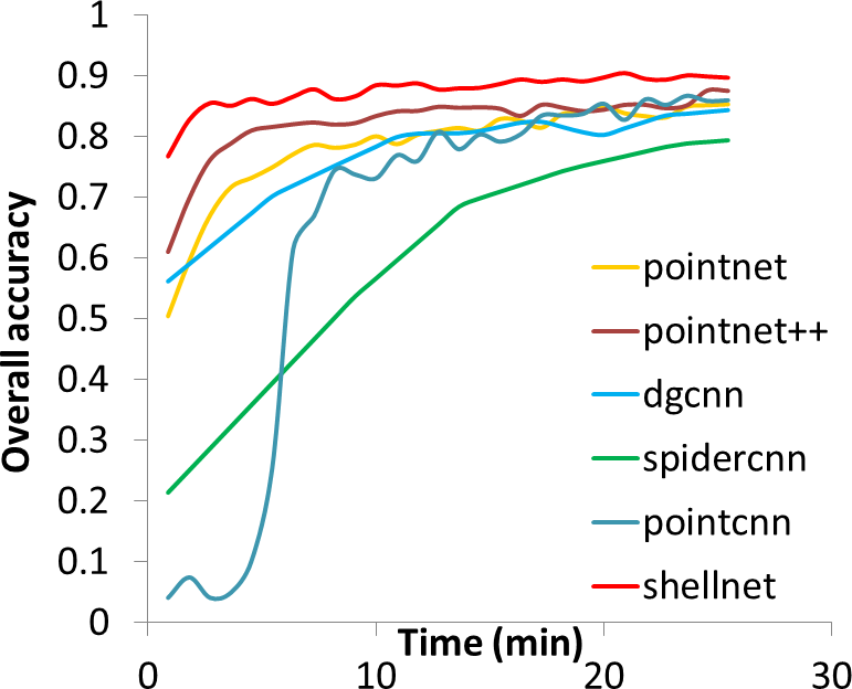
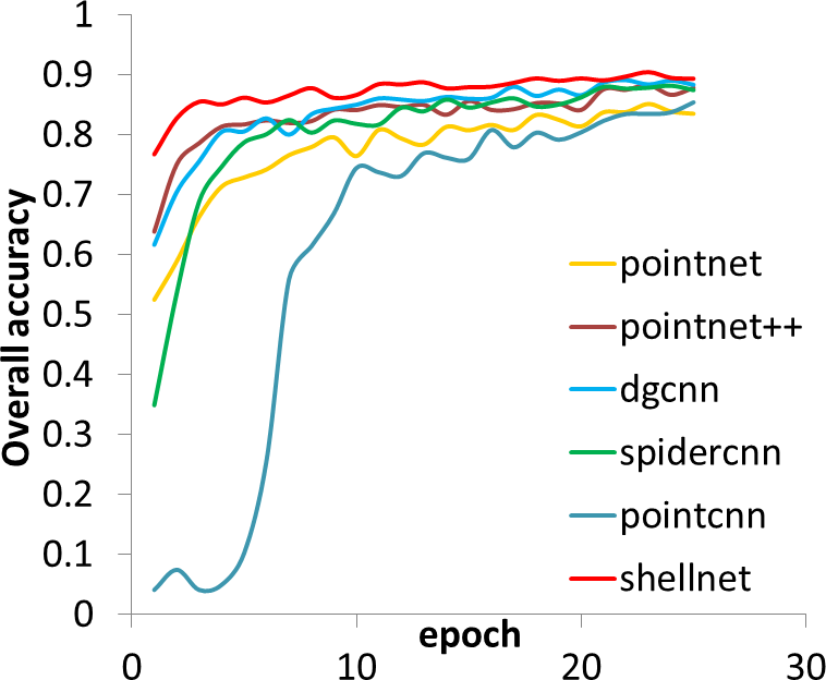
Figure 1: The accuracy of point cloud classification of different methods over time and epochs. While being accurate, some methods are quite costly to train. We address this problem by ShellConv, a simple yet effective convolutional operator based on concentric shell statistics. In both equal-time and equal-epoch comparisons, our method performs the best. It can achieve over 80% accuracy within two minutes, and reach 90% on the test dataset after only 15 minutes of training.

Recently, directly consuming point clouds using neural networks has shown great promises  [25, 27, 42, 20]. PointNet [25] pioneers this direction by learning with a symmetric function to make the network robust to point order ambiguity. Many subsequent works extend this direction by designing convolution that better captures local features of a point cloud. While such efforts lead to improved scene understanding performance, there is often a trade-off between network complexity, training speed, and accuracy. For example, the follow-up work PointNet++ [27] segments point cloud into smaller clusters and applies PointNet locally in a hierarchical manner. While achieving better result, the network is more complicated with reduced speed. Pointwise convolution [12] is simple to implement but inaccurate. SpiderCNN [42] extends traditional convolution on 2D images to 3D point clouds by parameterizing a family of convolution filters. Although high accuracy is achieved, more time is taken for training. PointCNN [20] achieves the state-of-the-art accuracy via learning a local convolution order but its training is slow to converge. In general, designing a convolution for point cloud that can strike a good balance between such performance factors is a challenging problem.

Based on these observations, we propose a novel approach to consume point clouds directly in a very simple neural network which is able to achieve the state-of-the-art accuracy with very fast training speed, as shown in Figure 1. Our idea is to split a local point neighborhood such that point neighboring and convolution with points can be performed efficiently. To achieve this, at each point, we query the point neighborhood and partition it with a set of concentric spheres, resulting in concentric spherical shells. In each shell, the representative features can be extracted based on the statistics of the points inside. By using ShellConv as the core convolution operator, an efficient neural network called ShellNet can be constructed to solve 3D scene understanding tasks such as object classification, object part segmentation, and semantic scene segmentation.

In general, the main contributions of this work are:

• ShellConv, a simple yet effective convolution operator for orderless point cloud. The convolution is defined on a domain that can be partitioned by concentric spherical shells, simultaneously allowing efficient neighbor point query and resolving point order ambiguity by defining a convolution order from the inner to the outer shells;

• ShellNet, an efficient neural network architecture based on ShellConv for learning with 3D point clouds directly without having any point order ambiguity;

• Applications of ShellNet on object classification, object part segmentation, and semantic scene segmentation that achieves the state-of-the-art accuracy.

2 Related Works

Recent advances in computer vision witness the growing availability of 3D scene datasets [2, 39, 44], leading to deep learning techniques to tackle the long-standing problem of scene understanding, particularly object classification, object part and scene segmentation. In this section, we review the state-of-the-art research in deep learning with 3D data, and then focus on techniques that enable feature learning on point clouds for scene understanding tasks.

Early deep learning with 3D data uses regular representations such as volumes [40, 23, 26, 21] and multi-view images [32, 26] for feature learning to solve object classification and semantic segmentation. Unfortunately, volume representation is very limited due to large memory footprints. Multi-view image representation does not have this issue, but it stores depth information implicitly, which makes it challenging to learn view-independent features.

Recently, deep learning in 3D focuses toward point clouds, which is more compact and intuitive compared to volumes. As point cloud is mathematically a set, using point cloud with deep neural networks requires fundamental changes to the core operator: convolution. Defining efficient convolution for point clouds has since been a challenging, but an important task. Inspired from learning with volumes, Hua et al. [12] perform on-the-fly voxelization at each point of the point cloud based on nearest point queries. Le et al. [17] propose to apply convolution on a regular grid with each cell containing point features that are resampled to a fixed size. Tatarchenko et al.  [33] perform convolution on the local tangent planes. Xie et al. [41] generalize shape context to convolution for point cloud. Liu et al. [22] use a sequence model to summarize local features with multiple scales. Such techniques lead to straightforward implementations of convolutional neural network for point clouds. However, extra computations are required for the explicit data representation, making the learning inefficient.

Instead of voxelization, it is possible to make neural network operate directly on point clouds. Qi et al. [25] propose PointNet, a pioneering network that learns global per-point features by optimizing a symmetric function to achieve point order invariance. The drawback of PointNet is that each point feature is learnt globally, i.e., no features from local regions are considered. Recent methods in point cloud learning are focused on designing convolution operators that can capture such local features.

In this trend, PointNet++ [27] supports local features by a hierarchy of PointNet, and relies on a heuristic point grouping to build the hierarchy. Li et al. [20] propose to learn a transformation matrix to turn the point cloud to a latent canonical representation, which can be further processed with standard convolutions. Xu et al. [42] propose to parameterize convolution kernels with a step function and Taylor polynomials. Wang et al. [38] propose a similar network structure to PointNet by optimizing weights between a point and its neighbors and using them for convolution. Shen et al. [30] also improve a PointNet-like network by kernel correlation and graph pooling. Huang et al. [13] learn the local structure particularly for semantic segmentation by applying traditional learning algorithms from recurrent neural networks. Ben-Shabat et al. [4] use a grid of spherical Gaussians with Fisher vectors to describe points. Such great efforts lead to networks with very high accuracies, but the efficiency of the learning is often overlooked (see Figure 1). This motivates us to focus on efficiency for local features learning in this work.

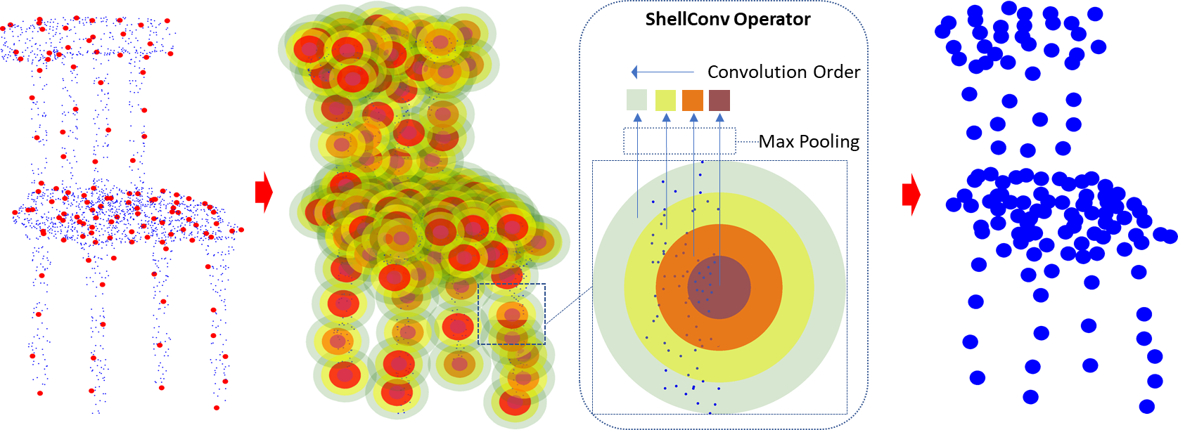
(a)          (b)          (c)            (d)

Figure 2: ShellConv operator. (a) For an input point cloud with/without associated features, representative points (red dots) are randomly sampled. The nearest neighbors are then chosen to form a point set centered at the representative points. The point sets are distributed across a series of concentric spherical shells (b) and the statistics of each shell is summarized by a maxpooling over all points in the shell, the features of which are lifted by an mlp to a higher dimension. The maxpooled features are indicated as squares with different colors (c). Following the inner to the outer order, a standard 1D convolution can be performed to yield the output features (d). Thicker dot means less points but each has higher dimensional features.

Beyond learning on unstructured point clouds, there have been some notable extension works, such as learning with hierarchical structures [28, 14, 35, 36], learning with self-organizing network [19], learning to map a 3D point cloud to a 2D grid [43, 8], addressing large-scale point cloud segmentation [15], handling non-uniform point cloud [11], and employing spectral analysis [45]. Such ideas are orthogonal to our method, and adding them on top of our proposed convolution could be an interesting future research.

3 The ShellConv Operator

To achieve an efficient neural network for point cloud, the first task is to define a convolution that is able to directly consume a point cloud. Our problem statement is given a set of points as input, define a convolution that can efficiently output a feature vector to describe the input point set.

There are two main issues when defining this convolution. First, the input point set has to be defined. It can be the entire point cloud, or a subset of the point cloud. The former case seeks a global feature vector that describes the entire point cloud; the latter seeks a local feature vector for each point set that can be further combined when needed. Second, one has to seamlessly take care of the point order ambiguity in a set and the density of the points in the point cloud. PointNet [25] opted to learn global features, but it has been shown by recent works [27, 20, 38, 42] that local features can lead to more representative features, resulting in better performance. We are motivated by these works and define a convolution to obtain features for a local point set. To keep our convolution simple but efficient, we propose an intuitive approach to addresses the challenges, below.

Algorithm 1 ShellConv Operator.

1:

2:$p$, $\Omega_{p}$, $\{F_{prev}(q):q\in\Omega_{p}\}$ * Representative point, point set, and previous layer features of point set.

3:$F_{p}$ * Convolutional features of $p$.

4:$\{q\}\leftarrow\{q-p:\forall q\in\Omega_{p}\}$ * Neighbor point $q$ is localised with $p$ as the center.

5:$\{F_{local}(q)\}\leftarrow\{\textrm{mlp}(q)\}$ * Individually lift each point $q$ to a higher dimensional space.

6:$\{F(q)\}\leftarrow\{[F_{prev}(q),F_{local}(q)\}$ * Concatenate the local and previous layer features.

7:$\{S\}\leftarrow\{S:q\in\Omega_{S}\}$ * Determine which shell $q$ belongs to according the distances from $q$ to center $p$.

8:$\{F(S)\}\leftarrow\{\mathrm{maxpool}(\{F(q):q\in\Omega_{S}\}):\forall S\}$ * Get fixed-size feature of each shell by a maxpool over all points in the shell.

9:$F_{p}\leftarrow\textrm{conv}(\{F(S)\})$ * Perform a 1D convolution with all shell features from inner to outer.

10:return $F_{p}$

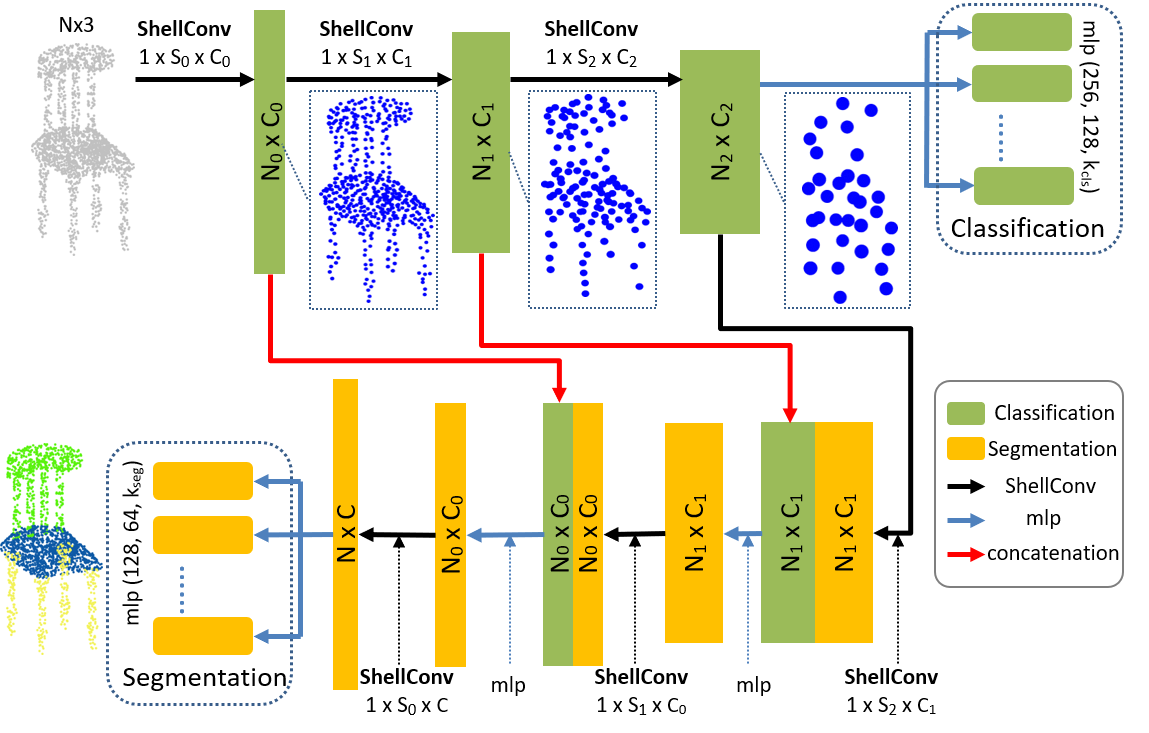
Figure 3: ShellNet architecture. For classification, we apply three layers of ShellConv before the fully connected classifier. For semantic segmentation, we follow a U-net [29] architecture. The encoder is in green and the decoder is in yellow. Point downsampling and upsampling is also included in our convolution, depending on its use. $N_{0}>N_{1}>N_{2}$ denotes the number of points in the input and after being sampled in each convolution, and $C<C_{0}<C_{1}<C_{2}$ denotes the output feature channels at each point. $S_{0}>S_{1}>S_{2}$ denotes the number of shells in each ShellConv operator that is analogous to the convolution kernel size. Given a fixed shell size, when the point cloud is downsampled, the number of shells also decreases. $1\times S_{0}\times C_{0}$ denotes a convolution that convolutes an input features using kernel $(1,S_{0})$ and output $C_{0}$ feature channels.

Convolution.

We show the main idea of our convolution in Figure 2. The common strategy in a traditional CNN architecture is to decrease the spatial resolution of the input and output more feature channels at deeper layers. We also support this strategy in our convolution by combining point sampling into the convolution, outputting sparser point sets at deeper layers. Different from previous works that stack many layers to increase receptive field, our method can obtain a larger receptive field without increasing the number of layers. Particularly, from the input point set, a set of representative points are randomly sampled (red dots in Figure 2 (a)). Each representative point and its neighbor points define a point set for convolution (Figure 2 (b)).

Let us now focus on a single representative point $p$ and its neighbors $q\in\Omega_{p}$, where $\Omega_{p}$ is the set of neighbors determined by a nearest neighbor query. By definition, the convolution at $p$ is

$$F(p)^{(n)}=\sum_{q\in\Omega_{p}^{(n)}}w(q)^{(n)}F(q)^{(n-1)}$$ (1)

where $F$ denotes the input feature of the point set for a particular channel, $w$ is the weight of the convolution. We use superscript ${(n)}$ to denote the data or parameters of layer $n$. Note that $F(p)$ and $F(q)$ denote the features of point $p$ and $q$. They are disregarded of the order of $p$ and $q$ in the point cloud because we simply treat the point cloud as a mathematical set. The only issue with this convolution here is how to define the weight function. The weights have to be suitable for training, i.e., $w$ has to be discretized into a fixed-size vector of trainable parameters. Defining $w$ for each point is not practical because the points are not ordered.

To address this issue, our observation here is that we can exploit the partitioning of the neighborhood into regions such that $w$ is well defined and the output can be computed efficiently. Particularly, to facilitate neighbor queries, we use a set of multi-scale concentric spheres to define the regions (Figure 2(c)). The region between two spheres forms a spherical shell. The union of the concentric spherical shells yields the domain $\Omega_{p}$. Therefore, we can define our convolution as

$$F(p)^{(n)}=\sum_{S\in\Omega_{p}^{(n)}}w_{S}^{(n)}F(S)^{(n-1)}$$ (2)

Note that as the shells are naturally ordered (from the inner most to the outermost), there is no ambiguity among the shells and the convolution is well defined, with weight $w_{S}$ for each shell. What remains ambiguous is the order of the points in the shells. To address this problem, we propose a statistical approach to aggregate features of the points in each shell such that it yields an order-invariant output. Particularly, we choose to represent the features by only the maximum value in each feature channel:

$$F(S)=\mathrm{maxpool}(\{F(q):q\in\Omega_{S}\})$$ (3)

where $\Omega_{S}$ denotes a shell $S$. Theoretically, the maximum value is a crude approximation to the underlying distribution, but because each point often has tens or hundreds of feature channels, the information from many points in the shell can still be represented. The detailed steps of ShellConv is presented in Algorithm 1.

Spherical Shells Construction.

We use a simple heuristics approach to establish the spherical shells as follows. We first compute the distance between the neighbor points to the representative point at the center. We then sort the distances, and distribute points to shells based on their distances to the center, from inner to outer. We assign a fixed number of points to each shell, i.e., $n$ points per shell in our implementation. Particularly, we first grow a sphere from the center until $n$ points falls inside the sphere. This is the innermost shell. After that, the sphere continues to grow to collect another $n$ points that forms the second shell, and so on. We found that this approach of shells construction provides a good stratification of point distributions in the shells. It is also easy to implement and has low overhead.

4 ShellNet

We now proceed to design a convolutional neural network for point cloud feature learning. We draw inspirations from typical 2D convolutional neural networks and build an architecture named ShellNet which uses ShellConv in place of traditional 2D convolution (see Figure 3). This architecture can be used for multiple scene understanding tasks. Particularly, the classification and segmentation networks both share the encoder part, and only differ in the part after that. Since ShellConv is permutation invariant for input points, ShellNet is able to consume point sets directly.

Our network for point cloud deep learning has three layers. In the classification stage, we pass all the input points through three ShellConv operators. The points are gradually subsampled into less representative points denoted as $N_{0}>N_{1}>N_{2}$ respectively, while the output feature channels increases layer by layer, denoted as $C_{0}<C_{1}<C_{2}$ respectively. In Figure 3, $N_{i}$ represented as blue dots with thicker shape that indicates a higher dimension. This design is similar to a typical 2D convolutional neural network: the number of representative points decreases while the number of output channels increases. After three layers of ShellConv, we obtain a matrix of size $N_{2}\times C_{2}$, where $N_{2}$ is the final number of representative points extracted from the input point cloud with each one contains a high dimensional feature vector of size $C_{2}$. This matrix is fed into the mlp module size of $(256,128)$ to produce the probability map for object classification. Finally, we obtain a $128\times k_{cls}$ matrix with $k_{cls}$ indicates the number of classes. The specific parameter settings are discussed in Section 5.1

The segmentation network follows U-net [29], an encoder-decoder architecture with skip connections. The deconvolution part starts with the set of $N_{2}$ points from the encoder, passing through the ShellConv operators until the point cloud reaches the original resolution. The deconvolution layers gradually output more points but less feature channels. Skip connections retain features from earlier layers and concatenate them to the output features of the deconvolution layers. Such strategy is shown to be highly effective for dense semantic segmentation on images [29], which we adopts here for point clouds. Note that we use ShellConv for both convolution and deconvolution. The output $N\times C$ is also fed into an mlp to produce the probability map for segmentation, where we obtain a $64\times k_{seg}$ matrix with $k_{seg}$ indicates the number of segment labels.

5 Experimental Results

In this section, we perform the experiments with three typical point cloud learning tasks: object classification, part segmentation, and semantic segmentation. We evaluate our method under different settings to justify the results. In general, our method achieves the state-of-the-art performance for both accuracy and speed in all the experiments.

5.1 Parameter Setting

ShellNet has three encoding layers, each of which contains a ShellConv. The parameters are $N_{i}$, $S_{i}$, and $C_{i}$ that denote the number of representative points, the number of shells, and output channels in each layer respectively. From the first to third layers, $N_{i}$ is set to 512, 128, 32, $S_{i}$ is set to 4, 2, 1, and $C_{i}$ is set to 128, 256, and 512 for $i=0,1,2$ respectively. $C$ is set to 64 at the last convolution for segmentation. We define the number of points contained in each shell as shell size, which is set to 16 for classification and 8 for segmentation. So the number of neighbors for each representative point is $S_{i}\times 16$ and $S_{i}\times 8$, which is equal to 64, 32, and 16 for the three layers of classification, and 32, 16, 8 for segmentation, respectively. During training, we use a batch size of $32$ for classification and $16$ for segmentation. The optimization is done with an Adam optimizer with initial learning rate set to 0.001. Our network is implemented in TensorFlow [1] and run on a NVIDIA GTX 1080 GPU for all experiments.

5.2 Object Classification

Method	Core Operator	input	OA
FPNN [21]	1D Conv.	P	87.5
Vol. CNN [26]	3D Conv.	V	89.9
O-CNN [35]	Sparse 3D Conv.	O	90.6
Pointwise [12]	Point Conv.	P	86.1
PointNet [25]	Point MLP	P	89.2
PointNet++ [27]	Multiscale Point MLP	P+N	90.7
PointCNN [20]	X-Conv	P	92.2
ShellNet ($ss$=8)	ShellConv	P	91.0
ShellNet ($ss$=16)	ShellConv	P	93.1
ShellNet ($ss$=32)	ShellConv	P	93.1
ShellNet ($ss$=64)	ShellConv	P	92.8

Table 1: Comparisons of classification accuracy (overall accuracy %) on ModelNet40 [40] with input type denoted as O (Octrees), V (Voxels), P (Points) and N (Normals). Performance of ShellNet is tested with different shell size ($ss$)

The classification is tested on ModelNet40 [40] which is composed of $40$ object classes and has $9,843$ models for training and $2,468$ models for testing. We use the point cloud data of ModelNet40 provided by Qi et al. [25] as input, where $1024$ points are roughly uniformly sampled from each mesh. Only the geometric coordinates $(x,y,z)$ of the sampled points are used in the experiment. We follow the train-test split from PointNet [25]. The data is augmented by randomly perturbing the point locations. The comparison results are shown in Table 1.

As we can see, our results have achieved the state-of-the-art. While ShellNet with shell size ($ss$) of 16 is the default setting for classification, other $ss$ are also tested. When decreasing $ss$ to 8, the receptive fields become smaller and less overlapped and accuracy also decreases slightly but still around $91.0\%$. When $ss$ increases, receptive field is enlarged so that more spatial context information is captured. ShellNet achieves $93.1\%$ accuracy with $ss$ is $32$. However, this does not mean the larger the better, since too large receptive field can also wash out the high frequency fine structure of the features [24]. We can see that when $ss$ is set to $64$, the accuracy drops to $92.8\%$. To balance between speed and accuracy, we set $ss$ to $16$ for object classification. Figure 1 provides an accuracy plot under equal-time and equal-epoch setting. As can be seen, our method outperformed all tested methods, being the fastest and most accurate towards convergence. Compared to PointCNN [20], one of the fastest method in this experiment, we use a much simpler network architecture. To turn the point cloud into a latent canonical representation, their X-Conv operator requires to learn a transformation matrix while our method only requires a statistical computation to aggregate features. This allows our convolution to be more intuitive and easy to implement but able to achieve high performance. We also provide per-class accuracy in the supplementary document.

5.3 Segmentation

Segmentation aims to predict the label for each point, which can also be seen as a dense pointwise classification problem. In this subsection, both object part segmentation and semantic scene segmentation are performed. We use ShapeNet dataset [44] for part segmentation, which contains $16,880$ models ($14,006$ models for training and $2,874$ models for testing) in $16$ categories, each annotated with $2$ to $6$ parts and there are $50$ different parts in total. For semantic segmentation, we use ScanNet [7] and S3DIS dataset [2] for indoor scenes, and Semantic3D [9] for outdoor scenes. ScanNet consists of 1513 RGB-D reconstructed indoor scenes annotated in 20 categories. S3DIS contains 3D scans from Matterport scanners in 6 indoor areas including 271 rooms with each point is annotated with one of the semantic labels from 13 categories. Semantic3D is an online large-scale, outdoor LIDAR benchmark dataset comprising more than 4 billion annotated points with 8 classes. We follow PointCNN [20] to prepare the datasets.

Object Part Segmentation. Our results are reported in Table 2. Per-class accuracies can be found in the supplementary document. It can be seen that our method outperforms most of the state-of-the-art techniques. Qualitative comparisons between our prediction and the ground truth are shown in Figure 4. It can be seen that ShellNet method can run robustly on many objects. Noted that our method only trains $20$ hours to achieve such accuracy.

Method	ShapeNet	ScanNet	S3DIS	Semantic3D
	mpIoU	OA	mIoU	mIoU
SyncCNN [45]	82.0	-	-	-
SpiderCNN [42]	81.7	-	-	-
SplatNet [31]	83.7	-	-	-
SO-Net [19]	81.0	-	-	-
SGPN [37]	82.8	-	50.4	-
PCNN [3]	81.8	-	-	-
KCNet [30]	82.2	-	-	-
KdNet [14]	77.4	-	-	-
3DmFV-Net [4]	81.0	-	-	-
DGCNN [38]	82.3	-	56.1	-
RSNet [13]	81.4	-	56.5	-
PointNet [25]	80.4	73.9	47.6	-
PointNet++ [27]	81.9	84.5	-	-
PointCNN [20]	84.6	85.1	65.4	-
TMLC-MSR [10]	-	-	-	54.2
DeePr3SS [16]	-	-	-	58.5
SnapNet [5]	-	-	-	59.1
SegCloud [34]	-	-	-	61.3
SPG [15]	-	-	62.1	73.2
Ours	82.8	85.2	66.8	69.4

Table 2: Comparisons of segmentation tasks. Object part segmentation is performed on ShapeNet dataset [6], and semantic segmentation is performed on ScanNet [7], S3DIS dataset [2], and Semantic3D [9] respectively.

Indoor Semantic Scene Segmentation. The mIoU accuracies of indoor benchmarks ScanNet [7] and S3DIS [2] are shown in Table 2. ShellNet ranks 1st on ScanNet and ranks 1st on S3DIS. For the latter, we also list the per-class scores (mIoU) in the supplementary document. The qualitative results are presented in Figure 5. We can see some misclassification are between wall, caseboard, and window as these categories are quite similar in pure geometries, and need other features like color or normal vectors to improve.

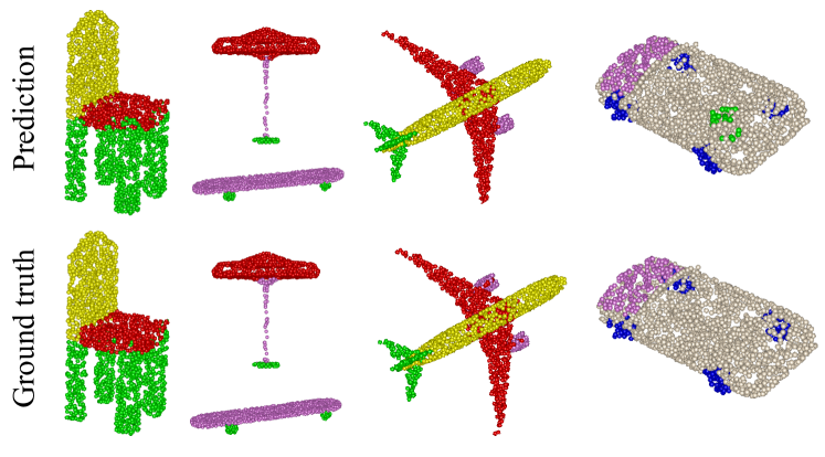
Figure 4: Object part segmentation with the ShapeNet dataset. The example objects are a chair, lamp, skateboard, airplane, and a car. Overall, our method produces accurate predictions.

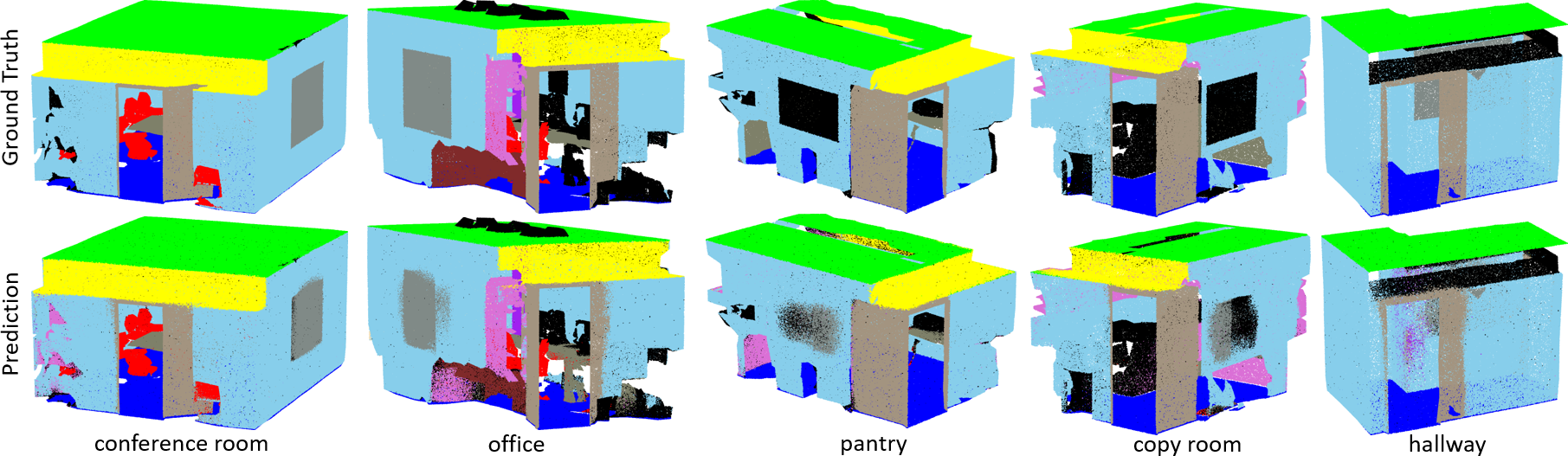
Figure 5: Semantic segmentation for indoor scenes in the S3DIS dataset [2].

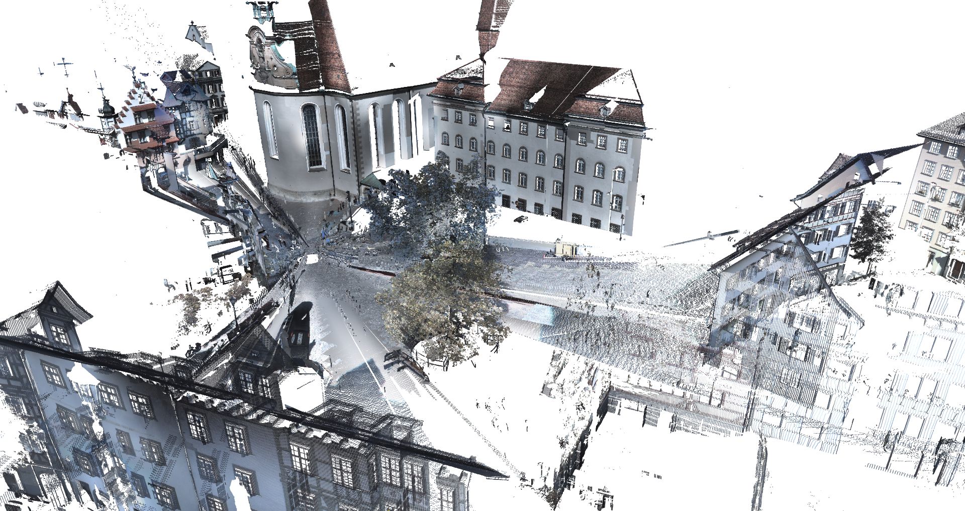
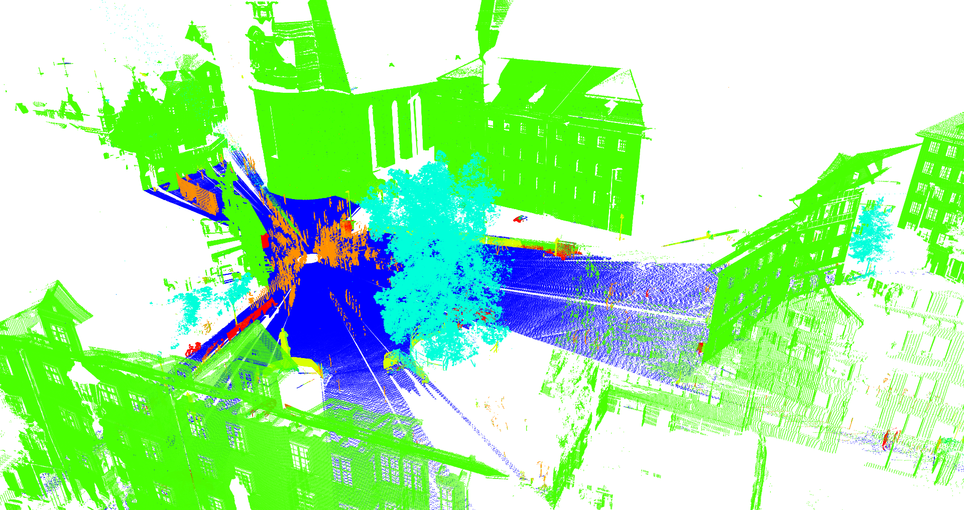
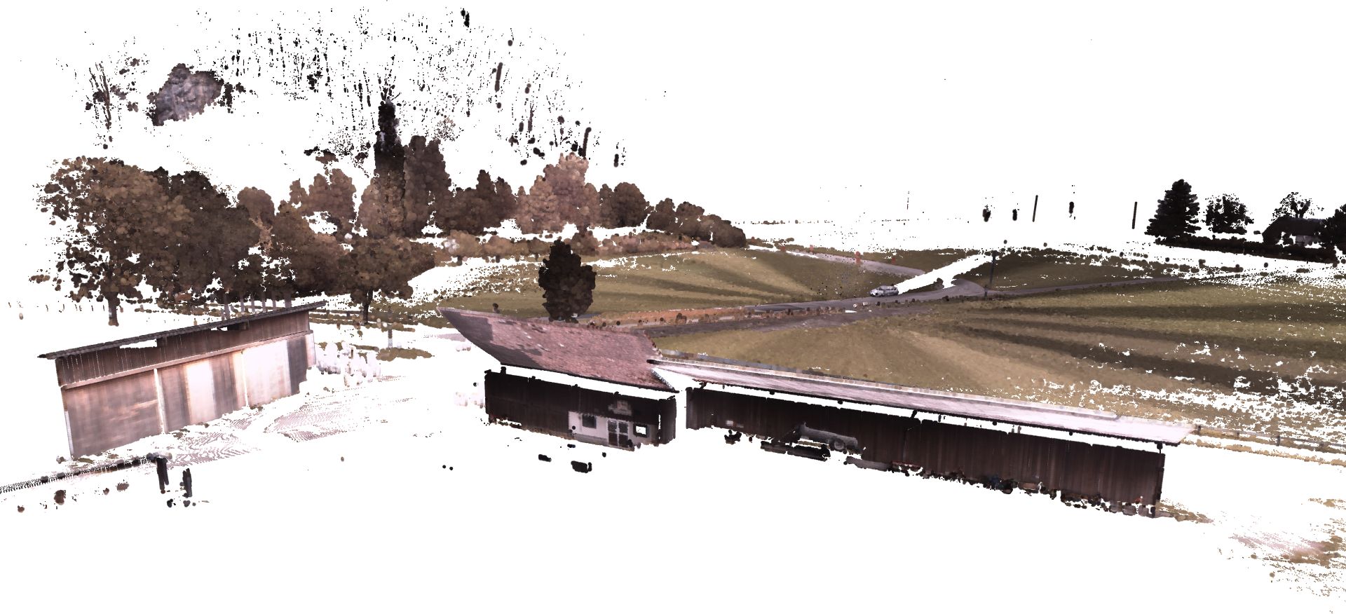
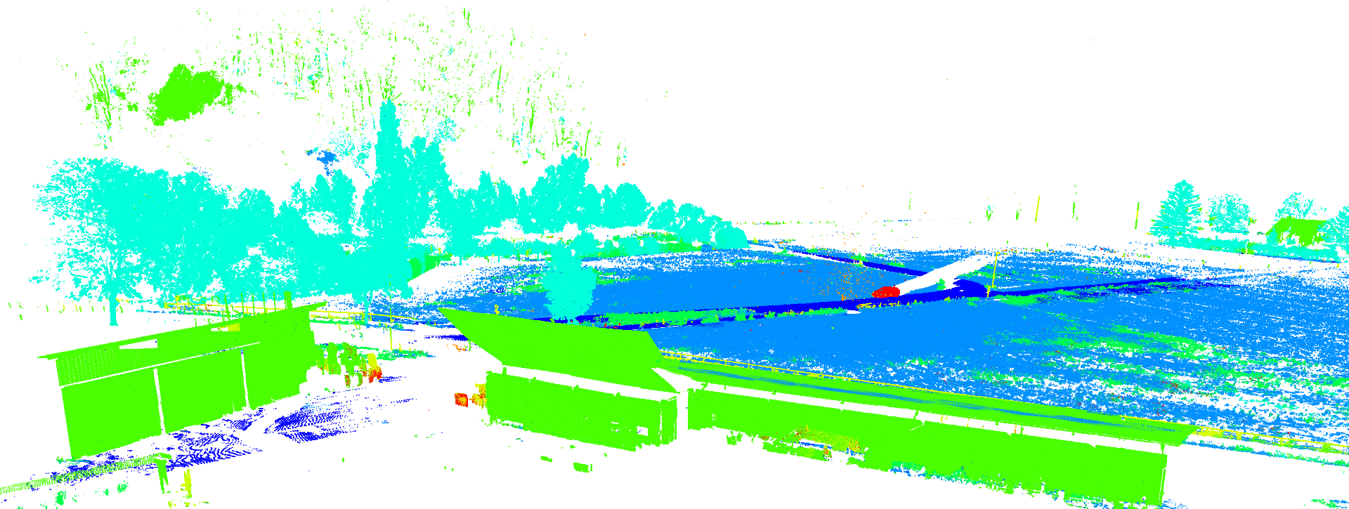
Figure 6: Semantic segmentation for outdoor scenes in the Semantic3D dataset [9]. Left: colored point clouds (for visualization only). Right: our segmentation. Note that the ground truth of the test set is not publicly available.

Outdoor Semantic Scene Segmentation. The Semantic3D [9] is more challenging as it is a real-world dataset of strongly varying point density. For a fair comparison, we excluded results without a publication. ShellNet performs well on this dataset with accuracy ranked 2nd (Table 2). Per-class accuracy can be found in the supplementary document. The qualitative results are presented in Figure 6. Note that our method only takes the 3D coordinates as input while previous methods such as [15] also used color or postprocess with CRFs.

5.4 Network Efficiency

We measure network complexity by the number of trainable parameters, floating point operations (FLOPs), and running time to analyze the network efficiency. With batch size 16, point cloud size 1024 from the ModelNet40 dataset, the statistics are reported in Table 3. For all three metrics, ShellNet is better than existing methods. While being much less complex in time and space, ShellNet can still converge to the state-of-the-art accuracy very efficiently as shown in the plot in Figure 1.

The improvement in speed and memory of our work comes from the effective use of mlp and 1D convolution in our network. Particularly, on top of the proposed systematic approach based on concentric shells for point grouping, which naturally handles multi-scale features, we only need a single mlp to learn point features in a shell, and a 1D convolution to relate features among the shells (Figure 2). This simplicity greatly reduces the number of trainable parameters and computation.

In ShellNet, the receptive field is directly controlled by the shell size. Thus, we can further analyse the performance of ShellNet with different shell sizes (Figure 7). In equal-time comparison, ShellNet with shell size 16 performs best, achieving high accuracy in very short time. When shell size is 64, it performs slightly worse. In equal-epoch setting, using shell size 8 is not as good as the others because of smaller receptive fields. Having a receptive field that balances between size and speed yields the best convergence.

Methods	Params	FLOPs	Time
		(Train/Infer)	(Train/Infer)
PointNet [25]	3.5M	44.0B / 14.7B	0.068s / 0.015s
PointNet++ [27]	12.4M	67.9B /26.9B	0.091s / 0.027s
3DmFV [4]	45.77M	48.6B /16.9B	0.101s / 0.039s
DGCNN [38]	1.84M	131.4B /44.3B	0.171s / 0.064s
PointCNN [20]	0.6M	93.0B /25.3B	0.031s / 0.012s
ShellNet	0.48M	15.8B /2.8B	0.066s / 0.023s
with small RF	0.48M	9.51B /1.5B	0.025s / 0.011s

Table 3: Trainable parameters, FLOPs and running time comparisons. Compared to previous methods, ShellNet is lightweight and fast while being accurate. Reducing the receptive field (small RF) by setting a smaller shell size can make the computation even faster as neighbor query becomes cheaper.

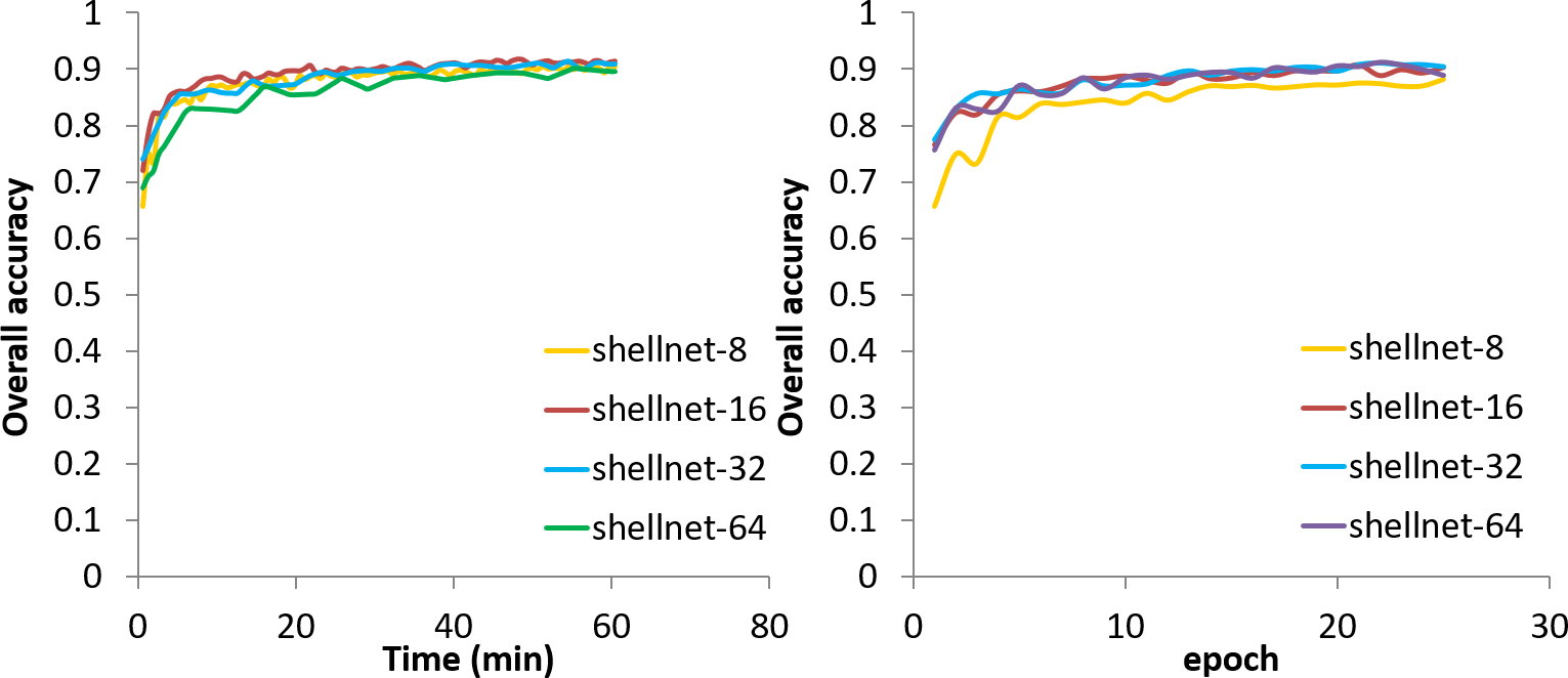
Figure 7: The accuracy of point cloud classification versus time and epochs with different shell sizes.

5.5 Neighboring Point Sampling

Let the network in Figure 3 as the baseline (Setting A), we conduct a series of experiments to verify the effectiveness of our network architecture and justify how neighbor points can be sampled.

Here we compare four settings. Particularly, Setting A is the default configuration of our classification experiment, in which random sampling is used to obtain neighbor points and each concentric shell contains a fixed number of points. Setting B, C, D are obtained by varying the neighbor sampling strategies. In Setting B, we change neighbor sampling to farthest point sampling. In Setting C, we divide a local region into equidistant shells, leading to shells that contain a dynamic number of points. In Setting D, we search nearest neighbors in the feature space instead of the 3D coordinate space. The results are shown in Table 4. It shows that accuracies are similar across variants, and Setting A is the most efficient for the classification task. For segmentation, we also conduct the same experiment and found that Setting B works best in this case. The reason is that farthest point sampling in Setting B results in more uniform point distribution that can cover more geometry details, leading to more accurate segmentation.

	(A)	(B)	(C)	(D)
1. Sampling	Random	Farthest	Random	Random
2. Shell size	Fixed	Fixed	Dynamic	Fixed
3. KNN type	$xyz$	$xyz$	$xyz$	Features
Accuracy (%)	93.1	93.1	92.7	92.4
Train Time	0.066s	0.078s	0.118s	0.081s
Infer. Time	0.023s	0.024s	0.033s	0.029s

Table 4: Experiments with neighbor point sampling. Setting (A) is the default strategy. Setting (B), (C), (D) are modified from (A) based on point sampling type, shell size, and neighbor query features. As can be seen, setting (B) – furthest point sampling, (C) – equidistant shells, (D) – latent features for neighborhood construction, produces similar accuracy but training and inference time becomes slower.

Our method is without limitation. Particularly, we found that while our method can work with sparse and partial data, more investigations into its robustness is required. Here we provide an example of object part segmentation to demonstrate the robustness of ShellConv in Figure 8. The mpIoU accuracies for the original, sparse and partial segmentation are 82.4%, 80.2%, 72.6% respectively. For partial data, the boundary points are less accurate.

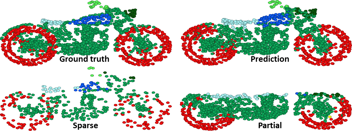
Figure 8: Part segmentation on sparse and partial point clouds. For partial data, points on the boundaries appear to be less accurate.

6 Conclusion

We introduced a novel approach for deep learning with 3D point clouds based on concentric spherical shells constructed from local point sets. We designed a new convolution operator named, ShellConv, which supports convolution of a point set efficiently based on shells and their statistics. This structure not only solves the convolution order problem naturally but also allows larger and more overlapped receptive field without increasing the number of network layers. Based on ShellConv, we build simple yet effective neural network that achieves the state-of-the-art results on object classification and segmentation tasks with pure point cloud inputs.

Together with recent advances in deep learning with point cloud data, our work leads to several potential future research. With the fast capability of local feature learning, it would be interesting to see how object detection and semantic instance segmentation can benefit from our work. It is also interesting to extend this work for learning with meshes. Finally, it would be of great interest to apply our approach to build autoencoders for point cloud generation.

Acknowledgements. The authors acknowledge support from the SUTD Digital Manufacturing and Design Centre funded by the Singapore National Research Foundation, and an internal grant from HKUST (R9429).

References

- [1] Martín Abadi, Paul Barham, Jianmin Chen, Zhifeng Chen, Andy Davis, Jeffrey Dean, Matthieu Devin, Sanjay Ghemawat, Geoffrey Irving, Michael Isard, et al. Tensorflow: A system for large-scale machine learning. In 12th USENIX Symposium on Operating Systems Design and Implementation (OSDI 16), pages 265–283, 2016.
- [2] Iro Armeni, Ozan Sener, Amir R Zamir, Helen Jiang, Ioannis Brilakis, Martin Fischer, and Silvio Savarese. 3d semantic parsing of large-scale indoor spaces. In Computer Vision and Pattern Recognition, pages 1534–1543, 2016.
- [3] Matan Atzmon, Haggai Maron, and Yaron Lipman. Point convolutional neural networks by extension operators. ACM Transactions on Graphics, 37(4), 2018.
- [4] Yizhak Ben-Shabat, Michael Lindenbaum, and Anath Fischer. 3dmfv: Three-dimensional point cloud classification in real-time using convolutional neural networks. IEEE Robotics and Automation Letters, 3:3145–3152, 2018.
- [5] Alexandre Boulch, Bertrand Le Saux, and Nicolas Audebert. Unstructured point cloud semantic labeling using deep segmentation networks. In Eurographics Workshop on 3D Object Retrieval, volume 2, page 7, 2017.
- [6] Angel X. Chang, Thomas A. Funkhouser, Leonidas J. Guibas, Pat Hanrahan, Qi-Xing Huang, Zimo Li, Silvio Savarese, Manolis Savva, Shuran Song, Hao Su, Jianxiong Xiao, Li Yi, and Fisher Yu. Shapenet: An information-rich 3d model repository. CoRR, abs/1512.03012, 2015.
- [7] Angela Dai, Angel X Chang, Manolis Savva, Maciej Halber, Thomas Funkhouser, and Matthias Niessner. Scannet: Richly-annotated 3d reconstructions of indoor scenes. In Computer Vision and Pattern Recognition, pages 5828–5839, 2017.
- [8] Thibault Groueix, Matthew Fisher, Vladimir G Kim, Bryan C Russell, and Mathieu Aubry. A papier-mâché approach to learning 3d surface generation. In Computer Vision and Pattern Recognition, pages 216–224, 2018.
- [9] Timo Hackel, Nikolay Savinov, Lubor Ladicky, Jan D Wegner, Konrad Schindler, and Marc Pollefeys. Semantic3d.net: A new large-scale point cloud classification benchmark. In ISPRS Annals of the Photogrammetry, Remote Sensing and Spatial Information Sciences, pages 91–98, 2017.
- [10] Timo Hackel, Jan D Wegner, and Konrad Schindler. Fast semantic segmentation of 3d point clouds with strongly varying density. ISPRS annals of the photogrammetry, remote sensing and spatial information sciences, 3(3):177–184, 2016.
- [11] Pedro Hermosilla, Tobias Ritschel, Pere-Pau Vázquez, Àlvar Vinacua, and Timo Ropinski. Monte carlo convolution for learning on non-uniformly sampled point clouds. ACM Transactions on Graphics, 2018.
- [12] Binh-Son Hua, Minh-Khoi Tran, and Sai-Kit Yeung. Point-wise convolutional neural network. In Computer Vision and Pattern Recognition, pages 984–993, 2018.
- [13] Qiangui Huang, Weiyue Wang, and Ulrich Neumann. Recurrent slice networks for 3d segmentation on point clouds. In Computer Vision and Pattern Recognition, pages 2626–2635, 2018.
- [14] Roman Klokov and Victor Lempitsky. Escape from cells: Deep kd-networks for the recognition of 3d point cloud models. In International Conference on Computer Vision, pages 863–872, 2017.
- [15] Loic Landrieu and Martin Simonovsky. Large-scale point cloud semantic segmentation with superpoint graphs. In Computer Vision and Pattern Recognition, pages 4558–4567, 2018.
- [16] Felix Järemo Lawin, Martin Danelljan, Patrik Tosteberg, Goutam Bhat, Fahad Shahbaz Khan, and Michael Felsberg. Deep projective 3d semantic segmentation. In International Conference on Computer Analysis of Images and Patterns, pages 95–107, 2017.
- [17] Truc Le and Ye Duan. Pointgrid: A deep network for 3d shape understanding. In Computer Vision and Pattern Recognition, pages 9204–9214, 2018.
- [18] Yann LeCun, Yoshua Bengio, and Geoffrey Hinton. Deep learning. Nature, 521(7553):436, 2015.
- [19] Jiaxin Li, Ben M Chen, and Gim Hee Lee. So-net: Self-organizing network for point cloud analysis. In Computer Vision and Pattern Recognition, pages 9397–9406, 2018.
- [20] Yangyan Li, Rui Bu, Mingchao Sun, Wei Wu, Xinhan Di, and Baoquan Chen. Pointcnn: Convolution on x-transformed points. In Advances in Neural Information Processing Systems, pages 820–830, 2018.
- [21] Yangyan Li, Soeren Pirk, Hao Su, Charles R Qi, and Leonidas J Guibas. Fpnn: Field probing neural networks for 3d data. In Advances in Neural Information Processing Systems, pages 307–315, 2016.
- [22] Xinhai Liu, Zhizhong Han, Yu-Shen Liu, and Matthias Zwicker. Point2sequence: Learning the shape representation of 3d point clouds with an attention-based sequence to sequence network. In Association for the Advancement of Artificial Intelligence, 2019.
- [23] Daniel Maturana and Sebastian Scherer. Voxnet: A 3d convolutional neural network for real-time object recognition. In International Conference on Intelligent Robots and Systems, pages 922–928, 2015.
- [24] Bartlett W. Mel and Stephen M. Omohundro. How receptive field parameters affect neural learning. In R. P. Lippmann, J. E. Moody, and D. S. Touretzky, editors, Advances in Neural Information Processing Systems, pages 757–763. Morgan-Kaufmann, 1991.
- [25] Charles R Qi, Hao Su, Kaichun Mo, and Leonidas J Guibas. Pointnet: Deep learning on point sets for 3d classification and segmentation. In Computer Vision and Pattern Recognition, pages 652–660, 2017.
- [26] Charles R Qi, Hao Su, Matthias Nießner, Angela Dai, Mengyuan Yan, and Leonidas J Guibas. Volumetric and multi-view cnns for object classification on 3d data. In Computer Vision and Pattern Recognition, pages 5648–5656, 2016.
- [27] Charles Ruizhongtai Qi, Li Yi, Hao Su, and Leonidas J Guibas. Pointnet++: Deep hierarchical feature learning on point sets in a metric space. In Advances in Neural Information Processing Systems, pages 5105–5114, 2017.
- [28] Gernot Riegler, Ali Osman Ulusoy, and Andreas Geiger. Octnet: Learning deep 3d representations at high resolutions. In Computer Vision and Pattern Recognition, pages 3577–3586, 2017.
- [29] Olaf Ronneberger, Philipp Fischer, and Thomas Brox. U-net: Convolutional networks for biomedical image segmentation. In International Conference on Medical image computing and computer-assisted intervention, pages 234–241. Springer, 2015.
- [30] Yiru Shen, Chen Feng, Yaoqing Yang, and Dong Tian. Mining point cloud local structures by kernel correlation and graph pooling. In Computer Vision and Pattern Recognition, pages 4548–4557, 2018.
- [31] Hang Su, Varun Jampani, Deqing Sun, Subhransu Maji, Evangelos Kalogerakis, Ming-Hsuan Yang, and Jan Kautz. SPLATNet: Sparse lattice networks for point cloud processing. In Computer Vision and Pattern Recognition, pages 2530–2539, 2018.
- [32] Hang Su, Subhransu Maji, Evangelos Kalogerakis, and Erik Learned-Miller. Multi-view convolutional neural networks for 3d shape recognition. In International Conference on Computer Vision, pages 945–953, 2015.
- [33] Maxim Tatarchenko, Jaesik Park, Vladlen Koltun, and Qian-Yi Zhou. Tangent convolutions for dense prediction in 3d. In Computer Vision and Pattern Recognition, pages 3887–3896, 2018.
- [34] Lyne Tchapmi, Christopher Choy, Iro Armeni, JunYoung Gwak, and Silvio Savarese. Segcloud: Semantic segmentation of 3d point clouds. In International Conference on 3D Vision, pages 537–547, 2017.
- [35] Peng-Shuai Wang, Yang Liu, Yu-Xiao Guo, Chun-Yu Sun, and Xin Tong. O-cnn: Octree-based convolutional neural networks for 3d shape analysis. ACM Transactions on Graphics, 36(4):72, 2017.
- [36] Peng-Shuai Wang, Chun-Yu Sun, Yang Liu, and Xin Tong. Adaptive o-cnn: A patch-based deep representation of 3d shapes. ACM Transactions on Graphics, 2018.
- [37] Weiyue Wang, Ronald Yu, Qiangui Huang, and Ulrich Neumann. Sgpn: Similarity group proposal network for 3d point cloud instance segmentation. In Computer Vision and Pattern Recognition, pages 2569–2578, 2018.
- [38] Yue Wang, Yongbin Sun, Ziwei Liu, Sanjay E. Sarma, Michael M. Bronstein, and Justin M. Solomon. Dynamic graph cnn for learning on point clouds. ACM Transactions on Graphics, 2019.
- [39] Zhirong Wu, Shuran Song, Aditya Khosla, Fisher Yu, Linguang Zhang, Xiaoou Tang, and Jianxiong Xiao. 3d shapenets: A deep representation for volumetric shapes. In Computer Vision and Pattern Recognition, pages 1912–1920, 2015.
- [40] Zhirong Wu, Shuran Song, Aditya Khosla, Fisher Yu, Linguang Zhang, Xiaoou Tang, and Jianxiong Xiao. 3d shapenets: A deep representation for volumetric shapes. In Computer Vision and Pattern Recognition, pages 1912–1920, 2015.
- [41] Saining Xie, Sainan Liu, Zeyu Chen, and Zhuowen Tu. Attentional shapecontextnet for point cloud recognition. In Computer Vision and Pattern Recognition, pages 4606–4615, 2018.
- [42] Yifan Xu, Tianqi Fan, Mingye Xu, Long Zeng, and Yu Qiao. Spidercnn: Deep learning on point sets with parameterized convolutional filters. In European Conference on Computer Vision, pages 87–102, 2018.
- [43] Yaoqing Yang, Chen Feng, Yiru Shen, and Dong Tian. Foldingnet: Point cloud auto-encoder via deep grid deformation. In Computer Vision and Pattern Recognition, pages 206–215, 2018.
- [44] Li Yi, Vladimir G. Kim, Duygu Ceylan, I-Chao Shen, Mengyan Yan, Hao Su, Cewu Lu, Qixing Huang, Alla Sheffer, and Leonidas Guibas. A scalable active framework for region annotation in 3d shape collections. ACM Transactions on Graphics, 2016.
- [45] Li Yi, Hao Su, Xingwen Guo, and Leonidas J Guibas. Syncspeccnn: Synchronized spectral cnn for 3d shape segmentation. In Computer Vision and Pattern Recognition, pages 2282–2290, 2017.