Shaping Lattice through irrelevant perturbation: Ising model

Abstract

The leading irrelevant perturbation, which controls the deviation of critical square lattice Ising model with periodic boundary conditions from its continuous CFT analog is identified. An explicit expression for the coupling constant in terms of the anisotropy parameter is found. We calculate the next to leading $\sim 1/N^{2}$ corrections to the spectrum on both lattice theory and the perturbed CFT sides for several classes of states, always getting exact agreement. We discuss also how the perturbing operators and the higher integrals of motion are related.

1 Introduction

It is well known that large scale behavior of many statistical systems near their critical points can be described by (Euclidean) Quantum Field Theories (QFT) (see e.g. domb1972phaseV6 ). In such description many microscopic details of initial theory are washed out, so that various statistical systems may lead to the same continuous theory. In this respect it is interesting to investigate intermediate scales, where some subleading corrections (besides leading finite size effects) to the QFT description still are noticeable. Then it would be possible to clarify how specific microscopic structure of the system is reflected in this corrections. From QFT point of view such corrections can be described as perturbations by irrelevant operators which are allowed to carry nonzero spins, since the rotational invariance at small distances is violated domb1987phaseV11 ; CARDY1986200 . In this respect the two dimensional Ising model Ising:1925em is an ideal object to investigate, since it is exactly integrable Onsager . Moreover, for some boundary conditions all the eigenvalues of its transfer matrix are known exactly even for finite lattices (see e.g. baxter2007exactly for toroidal boundary conditions, Brien for several other cases).

The paper is organized as follows.

In section 2 we systematically investigate the eigenvalues of periodic critical Ising transfer-matrix in large $L$ limit ($L$ is the number of spins in a horizontal row). We show how $1/L$ terms exactly match with CFT prediction and compute the next $1/L^{3}$ corrections for certain families of eigenvalues. The $1/L^{3}$ corrections under discussion describe breakdown of rotational invariance due to lattice artifacts.

In section 3 we address the question, how to perturb Ising CFT in order to get precisely those corrections which we obtained investigating lattice model. We were able to identify the perturbing fields and the respective coupling constants. Namely we show that the perturbing fields are the spin $4$ current and its antiholomorphic counterpart, which were introduced in the context of integrable structure of CFT long ago. Having non-zero spin, these fields break the rotational invariance, while being irrelevant, they slightly correct the large distance behavior in a way, to mimic the lattice result.

Finally we end up with a summary of our results and discuss the possibility of generalization for full spectrum and for higher order corrections.

2 Eigenvalues of the transfer matrix

Consider square lattice Ising model. We’ll adopt the ”$45$ degree rotated” version presented in great details e.g. in Baxter’s seminal book baxter2007exactly . The lattice consists of $L$ vertical columns of $L^{\prime}$ faces, or equivalently, of $L^{\prime}$ horizontal rows of $L$ faces (see Fig.1). We will consider periodic boundary condition in both, horizontal and vertical directions, so that the $L+1$-th column is identified with the first column and the $L^{\prime}+1$-th row with the first one.

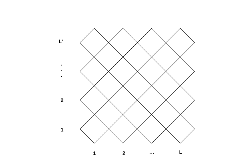
Figure 1: Periodic Ising Lattice. The leftmost (lowermost) spins are identified with corresponding rightmost (uppermost) spins.

The partition function of the theory is given by

$$Z=\sum_{\{\mathbf{\sigma}\}}\exp\left(J\sum_{\langle i,j\rangle}\sigma_{i}\sigma_{j}+K\sum_{\langle k,l\rangle}\sigma_{i}\sigma_{j}\right),$$ (2.1)

where $\langle i,j\rangle$ belong to the set of SW-NE, and $\langle k,l\rangle$ to the NW-SE edges. In what follows, we will restrict ourselves to the case of critical Ising model. The well known criticality condition $\sinh 2J\sinh 2K=1$ can be conveniently parameterized by a single parameter $u$ by setting

$$\sinh 2J=\cot 2u\,;\qquad\sinh 2K=\tan 2u\,,$$ (2.2)

with $0<u<\pi/4$. Sometimes the parameter $u$ is referred as the anisotropy. The value $u=\pi/8$ corresponds to the isotropic case.

To define the transfer matrix of the model, let us denote the Boltzmann weights of two basic types of three spin configurations shown in Fig.2 as

$$W\left(\begin{array}[]{ll}\sigma_{1}&\\[-10.0pt] &\sigma_{3}\\[-10.0pt] \sigma_{2}&\end{array}\right)\qquad\text{and}\qquad W\left(\begin{array}[]{ll}&\sigma_{1}\\[-10.0pt] \sigma_{3}&\\[-10.0pt] &\sigma_{2}\end{array}\right)\,,$$ (2.9)

where $\sigma_{i}=\pm 1$ are the Ising spins. Thus, the arrangement of spins in the argument of $W$ follows to the geometric pattern of their locations on the lattice.

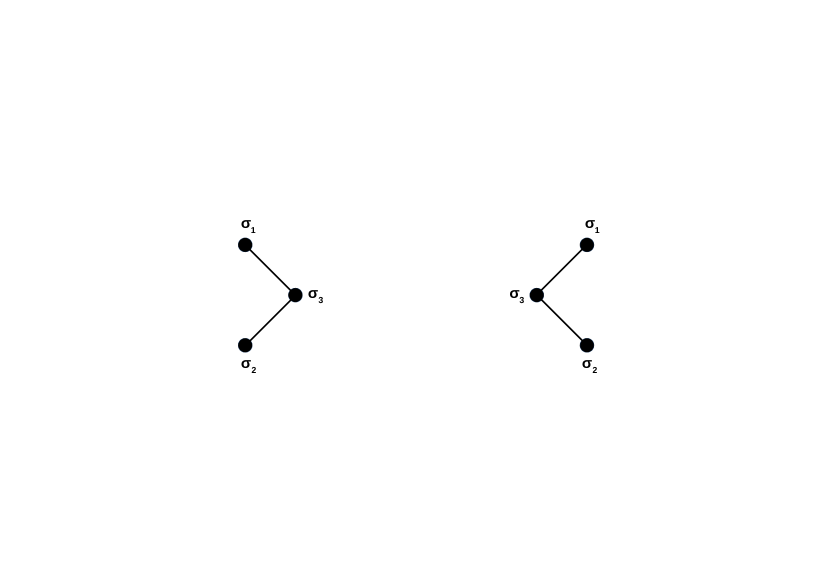
Figure 2: Two basic configurations of three Ising spins.

These Boltzmann weights are explicitly given by

$$W\left(\begin{array}[]{ll}\sigma&\\[-10.0pt] &\sigma\\[-10.0pt] \sigma&\end{array}\right) = W\left(\begin{array}[]{ll}&\sigma\\[-10.0pt] \sigma&\\[-10.0pt] &\sigma\end{array}\right)=\sqrt{2}\cos(u)\cos\left(\frac{\pi}{4}-u\right)\,,$$ (2.16)

$$W\left(\begin{array}[]{ll}\sigma&\\[-10.0pt] &-\sigma\\[-10.0pt] \sigma&\end{array}\right) = W\left(\begin{array}[]{lr}&\sigma\\[-10.0pt] -\sigma&\\[-10.0pt] &\sigma\end{array}\right)=\sqrt{2}\sin(u)\sin\left(\frac{\pi}{4}-u\right)\,,$$ (2.23)

$$W\left(\begin{array}[]{rl}\sigma&\\[-10.0pt] &\sigma\\[-10.0pt] -\sigma&\end{array}\right) = W\left(\begin{array}[]{cr}&-\sigma\\[-10.0pt] \sigma&\\[-10.0pt] &\sigma\end{array}\right)=\sqrt{2}\sin(u)\cos\left(\frac{\pi}{4}-u\right)$$ (2.30)

$$W\left(\begin{array}[]{rc}-\sigma&\\[-10.0pt] &\sigma\\[-10.0pt] \sigma&\end{array}\right) = W\left(\begin{array}[]{rr}&\sigma\\[-10.0pt] \sigma&\\[-10.0pt] &-\sigma\end{array}\right)=\sqrt{2}\sin\left(\frac{\pi}{4}-u\right)\cos(u)\,,$$ (2.37)

where $\sigma=\pm 1$ and $u$ is the anisotropy parameter. Note that to get (2.37) from (2.2), one should include an overall extra factor $\frac{1}{2}\sqrt{\sin 4u}$. Such shift in vacuum energy is convenient particularly because the transfer matrix, defined below, becomes the one-step shift operator at the values $u=0$ and $u=\frac{\pi}{4}$.

After imposing periodic boundary condition in horizontal direction for the transfer-matrix we get (See Fig.3)

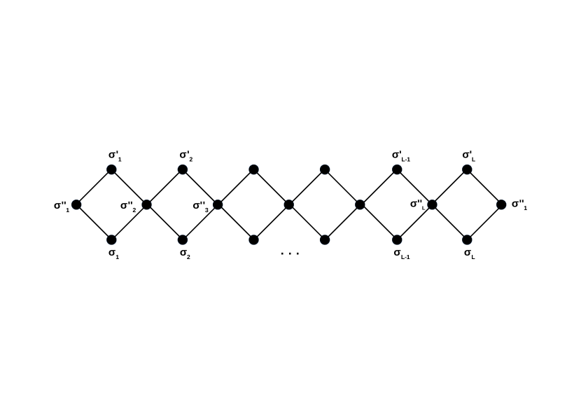
Figure 3: The transfer matrix. Sum over all middle spins $\sigma^{\prime\prime}$ is assumed

$$T_{\mathbf{\sigma},\mathbf{\sigma}^{\prime}}=\sum_{\mathbf{\sigma}^{\prime\prime}}W\left(\begin{array}[]{ll}&\sigma_{1}^{\prime}\\[-10.0pt] \sigma_{1}^{\prime\prime}&\\[-10.0pt] &\sigma_{1}\end{array}\right)W\left(\begin{array}[]{ll}\sigma_{1}^{\prime}&\\[-10.0pt] &\sigma_{2}^{\prime\prime}\\[-10.0pt] \sigma_{1}&\end{array}\right)W\left(\begin{array}[]{ll}&\sigma_{2}^{\prime}\\[-10.0pt] \sigma_{2}^{\prime\prime}&\\[-10.0pt] &\sigma_{2}\end{array}\right)\cdots W\left(\begin{array}[]{ll}\sigma_{L}^{\prime}&\\[-10.0pt] &\sigma_{1}^{\prime\prime}\\[-10.0pt] \sigma_{L}&\end{array}\right)$$ (2.50)

The exact eigenvalues of this transfer-matrix can be found in baxter2007exactly . We will use a slightly modified version of the explicit expressions, presented in Brien based on more general treatment of Behrend:1995zj (see also later works Behrend1 ; Pearce2001 ; Chui ). There are two sets of eigenvalues, distinguished by the parameter $r=\pm 1$ and denoted by $\Lambda^{(\pm)}$ respectively. To be precise, let me warn the reader, that the quantities $\Lambda^{(\pm)}$ introduced below, actually are the square roots of transfer matrix eigenvalues. Nevertheless with a slight abuse of terminology, they will be referred simply as eigenvalues.

For $r=1$ the set of eigenvalues are given explicitly as Brien ($\lfloor x\rfloor$ stands for the largest integer not exceeding $x$):

$$\Lambda^{(+)}(\mu_{k},\bar{\mu}_{k})=\sqrt{2}\left(2e^{2iu+\frac{i\pi}{4}}\right)^{-L}\prod_{k=1}^{\lfloor\frac{L}{2}\rfloor}\left(i\mu_{k}\tan\left(\frac{\pi(2k-1)}{4L}\right)+e^{4iu}\right)$$

$$\prod_{k=1}^{\lfloor\frac{L+1}{2}\rfloor}\left(i\cot\left(\frac{\pi(2k-1)}{4L}\right)+e^{4iu}\bar{\mu}_{k}\right),$$ (2.51)

where $\mu_{k},\,\,\bar{\mu}_{k}\in\{+1,-1\}$ are subject to the constraint

$$\prod_{k=1}^{\lfloor\frac{L}{2}\rfloor}\mu_{k}\prod_{k=1}^{\lfloor\frac{L+1}{2}\rfloor}\bar{\mu}_{k}=1$$ (2.52)

For $r=-1$ we have another set of eigenvalues Brien :

$$\Lambda^{(-)}(\mu_{k},\bar{\mu}_{k})=\sqrt{1+L}\left(2e^{2iu+\frac{i\pi}{4}}\right)^{-L}\prod_{k=1}^{\lfloor\frac{L}{2}\rfloor}\left(i\mu_{k}\tan\left(\frac{\pi k}{2L}\right)+e^{4iu}\right)$$

$$\prod_{k=1}^{\lfloor\frac{L-1}{2}\rfloor}\left(i\cot\left(\frac{\pi k}{2L}\right)+e^{4iu}\bar{\mu}_{k}\right);$$ (2.53)

where again $\mu_{k},\,\,\bar{\mu}_{k}\in\{+1,-1\}$, but there is no constraint anymore.

Notice that altogether we get $2^{L-1}+2^{L-1}=2^{L}$ eigenvalues, which exactly matches the size of transfermatrix (2.50).

2.1 Leading Eigenvalues

The leading eigenvalues in both sectors correspond to the case when all $\mu_{k}=+1$, $\bar{\mu}_{k}=+1$. The expressions for these eigenvalues can be simplified and represented as

$$\left(\Lambda^{(+)}_{max}\right)^{2}=\prod_{k=0}^{L-1}\left(\sin(4u)\sin\left(\frac{\pi k}{L}+\frac{\pi}{2L}\right)+1\right)$$ (2.54)

and

$$\left(\Lambda^{(-)}_{max}\right)^{2}=\prod_{k=0}^{L-1}\left(\sin(4u)\sin\left(\frac{\pi k}{L}\right)+1\right)$$ (2.55)

2.2 CFT prediction

From now on instead of parameters $L$ and $L^{\prime}$ we’ll use the even integers

$$N=2L\quad\text{and}\quad M=2L^{\prime},$$

which are the numbers of vertical and horizontal ”zigzagging” columns and rows of the lattice respectively (see Fig.1). Conformal field theory predicts that the logarithm of transfer matrix eigenvalues in large $N$, $M$ limit behave as PhysRevLett.56.742 ; PhysRevLett.56.746

$$M\log\Lambda\sim-\frac{NM}{2}\,f_{bulk}+\left(\Delta-\frac{c}{24}\right)\log q+\left(\bar{\Delta}-\frac{c}{24}\right)\log\bar{q},$$ (2.56)

where $f_{bulk}$ is the free energy per site (the number of sights in our lattice is $\frac{NM}{2}$), $\Delta$, $\bar{\Delta}$ are the left and right dimensions of the conformal field which creates the corresponding eigenstate from the vacuum. The parameter $q=\exp 2\pi i\tau$, where $\tau$ is modulus of the torus on which our 2d CFT lives, should be identified as

$$2\pi i\tau=\log q=-\frac{2\pi iM\,e^{-4iu}}{N}$$ (2.57)

Finally, $c$ is the Virasoro central charge, which for our case of Ising model, assumes the value $c=1/2$.

Notice also that besides finite size scaling, CFT predicts also the universal amplitude ratios (see e.g. Salas:1999qh and references therein).

2.3 Large $N$ expansion of leading eigenvalues

Denote

$$f(x)=\log(1+\sin(4u)\sin(x))$$ (2.58)

and $h=\frac{2\pi}{N}$. Due to Euler-Maclaurin summation formula ($B_{n}(\alpha)$ are the Bernoulli polynomials) from eq. (2.54) we get

$$\log\Lambda^{(+)}_{max}+\frac{N}{2}\,f_{bulk}=\sum_{n=1}^{\infty}\frac{B_{n}\left(\frac{1}{2}\right)\left(f^{(n-1)}(\pi)-f^{(n-1)}(0)\right)h^{n-1}}{n!}$$

$$=\frac{\pi\sin(4u)}{12N}+\frac{7\pi^{3}\left(2\sin(4u)-4\sin^{3}(4u)\right)}{1440N^{3}}+O(1/N^{5})$$ (2.59)

and from (2.55)

$$\log\Lambda^{(-)}_{max}+\frac{N}{2}f_{bulk}=\sum_{n=1}^{\infty}\frac{B_{n}\left(0\right)\left(f^{(n-1)}(\pi)-f^{(n-1)}(0)\right)h^{n-1}}{n!}$$

$$=-\frac{\pi\sin(4u)}{6N}-\frac{\pi^{3}\left(2\sin(4u)-4\sin^{3}(4u)\right)}{180N^{3}}+O(1/N^{5})$$ (2.60)

The bulk free energy is given by

$$f_{bulk}=-\int_{0}^{\pi}f(x)\,\frac{dx}{2\pi}.$$ (2.61)

Taking into account that the leading eigenvalue should correspond to the identity operator with conformal dimensions $\Delta=\bar{\Delta}=0$, consistency of the leading terms in (2.59), (2.60) with CFT prediction (2.56) immediately fixes the value of central charge $c=1/2$ and identifies the torus parameter $q$ with the expression (2.57). Besides for the dimensions of the conformal field corresponding to the eigenvalue $\Lambda^{(-)}_{max}$ we get $\Delta=\bar{\Delta}=1/16$, which are the correct dimensions of Ising spin field.

2.4 Partition function on a large torus and Ising fermions

For given $p$, denote $\Lambda^{(+)}_{p}$ ($\bar{\Lambda}^{(+)}_{p}$) the rhs of (2.51) for the case when $r=1$ with all $\mu$’s and $\bar{\mu}$’s set to $1$ with a single exception, namely $\mu_{p}=-1$ ($\bar{\mu}_{p}=-1$). Analogously, using (2.53), we define $\Lambda^{(-)}_{p}$, $\bar{\Lambda}^{(-)}_{p}$ for the case when $r=-1$. In large $N$ limit the impact of flipping the sign at position $p$ are given by ratios

$$\log\frac{\Lambda^{(+)}_{p}}{\Lambda^{(+)}_{max}} = -\frac{i\pi(2p-1)e^{-4iu}}{N}-\frac{i\pi^{3}(2p-1)^{3}e^{-4iu}\left(1-e^{-8iu}\right)}{12N^{3}}+O\left(1\over N^{5}\right)$$

$$\log\frac{\bar{\Lambda}^{(+)}_{p}}{\Lambda^{(+)}_{max}} = \frac{i\pi(2p-1)e^{4iu}}{N}+\frac{i\pi^{3}(2p-1)^{3}e^{4iu}\left(1-e^{8iu}\right)}{12N^{3}}+O\left(1\over N^{5}\right)$$ (2.62)

and

$$\log\frac{\Lambda^{(-)}_{p}}{\Lambda^{(-)}_{max}} = -\frac{2i\pi pe^{-4iu}}{N}-\frac{2i\pi^{3}p^{3}e^{-4iu}\left(1-e^{-8iu}\right)}{3N^{3}}+O\left(1\over N^{5}\right)$$

$$\log\frac{\bar{\Lambda}^{(-)}_{p}}{\Lambda^{(-)}_{max}} = \frac{2i\pi pe^{4iu}}{N}+\frac{2i\pi^{3}p^{3}e^{4iu}\left(1-e^{8iu}\right)}{3N^{3}}+O\left(1\over N^{5}\right)$$ (2.63)

It is important to notice that due to factorized structure of eigenvalues (2.51) and (2.53), if there are several indices $p_{1},p_{2},\cdots$, such that the respective $\mu$’s or $\bar{\mu}$’s assume the value $-1$, the logarithm of ratios of eigenvalues will be given by the same expressions (2.62) and (2.63) summed over above specified indices p.

Consider thermodynamic limit when $M$, $N$ are sent to infinity while keeping their ratio fixed. Notice that $q$, $\bar{q}$ remain finite as seen from (2.57). Keeping the leading terms only, we can conveniently rewrite expressions (2.62), (2.63) in view of eq. (2.57) as

$$\left(\frac{\Lambda^{(+)}_{p}}{\Lambda^{(+)}_{max}}\right)^{M}\sim q^{p-\frac{1}{2}};\,\,\,\left(\frac{\Lambda^{(-)}_{p}}{\Lambda^{(+)}_{max}}\right)^{M}\sim q^{\bar{p}-\frac{1}{2}};\,\,\,\left(\frac{\bar{\Lambda}^{(+)}_{p}}{\Lambda^{(-)}_{max}}\right)^{M}\sim q^{p};\,\,\,\left(\frac{\Lambda^{(-)}_{p}}{\Lambda^{(-)}_{max}}\right)^{M}\sim\bar{q}^{p}\qquad$$ (2.64)

In other words, the sign flip of $\mu_{p}$ ( $\bar{\mu}_{p}$) in partition sum costs a multiplier $q^{p-\frac{1}{2}}$ ($\bar{q}^{p-\frac{1}{2}}$) in the $r=1$ sector and a multiplier $q^{p}$ ($\bar{q}^{p}$) in the sector $r=-1$. We’ll need also the contributions of the eigenvalues $\Lambda^{(\pm)}_{max}$ in partition function. Again, dropping $O(1/N^{3})$ terms, from eqs. (2.59), (2.60) we easily get

$$\left(\Lambda^{(+)}_{max}\right)^{M}\sim e^{-MNf_{bulk}/2}(q\bar{q})^{-\frac{1}{48}};\qquad\left(\Lambda^{(-)}_{max}\right)^{M}\sim e^{-MNf_{bulk}/2}(q\bar{q})^{-\frac{1}{48}+\frac{1}{16}}.$$

As a result, a generic eigenvalue, say in sector $r=-1$, specified by conditions $\mu_{p_{1}}=\mu_{p_{2}}=\cdots=\mu_{p_{R}}=-1$, $\bar{\mu}_{\tilde{p}_{1}}=\bar{\mu}_{\tilde{p}_{2}}=\cdots=\bar{\mu}_{\tilde{p}_{L}}=-1$ with all other $\mu$’s and $\bar{\mu}$’s taking the value $1$, will contribute a term

$$e^{-MNf_{bulk}/2}(q\bar{q})^{-\frac{1}{48}+\frac{1}{16}}q^{p_{1}}q^{p_{2}}\cdots q^{p_{R}}\bar{q}^{\tilde{p}_{1}}\bar{q}^{\tilde{p}_{2}}\cdots\bar{q}^{\tilde{p}_{L}}$$

Similarly, the contribution of a generic eigenvalue from the sector $r=-1$ in partition function reads

$$e^{-MNf_{bulk}/2}(q\bar{q})^{-\frac{1}{48}+\frac{1}{16}}q^{p_{1}-1/2}q^{p_{2}-1/2}\cdots q^{p_{R}-1/2}\bar{q}^{\tilde{p}_{1}-1/2}\bar{q}^{\tilde{p}_{2}-1/2}\cdots\bar{q}^{\tilde{p}_{L}-1/2}.$$

Here we should keep in mind that due to the constraint (2.52), the total number of minus signs, i.e. $R+L$ must be even. Now, by elementary considerations one can get convinced that the partition function on the torus in continuum limit can be represented as

$$Z\sim e^{-MNf_{bulk}/2}(q\bar{q})^{-\frac{1}{48}}\hskip 227.62204pt$$

$$\times\left(\frac{1}{2}\prod_{k=1}^{\infty}\left(1+q^{k-\frac{1}{2}}\right)\left(1+\bar{q}^{k-\frac{1}{2}}\right)+\frac{1}{2}\prod_{k=1}^{\infty}\left(1-q^{k-\frac{1}{2}}\right)\left(1-\bar{q}^{k-\frac{1}{2}}\right)\right.$$

$$\left.+(q\bar{q})^{\frac{1}{16}}\prod_{k=1}^{\infty}\left(1+q^{k}\right)\left(1+\bar{q}^{k}\right)\right).$$ (2.65)

Note that the sum with factors $1/2$ on second line implements the constraint (2.52), since the terms with a product of odd number of minus signs get canceled.

Obviously, the form of (2.65) reflects the well known fact that the Ising model in continuous limit is the theory of free fermions. The fermionic fields are single valued in vacuum sector (manifested by the half integer modes on second line of (2.65)), while they are non-local with respect to the spin field and have integer modes as seen on third line of (2.65). Let us briefly recall few relevant facts about free fermion theory. We will simply state the results omitting details and proofs. The aim is to specify notations which will be used later on. A comprehensive review of 2d fermion CFT can be found e.g. in book DiFrancesco:639405 . The left and right moving fermion fields can be defined through mode expansions

$$\psi(z)=\sum_{\nu}\frac{\psi_{\nu}}{z^{\nu+\frac{1}{2}}}$$ (2.66)

$$\bar{\psi}(\bar{z})=\sum_{\nu}\frac{\bar{\psi}_{\nu}}{\bar{z}^{\nu+\frac{1}{2}}}$$ (2.67)

where sum is over all half integers or over all integers, depending whether it acts in vacuum sector (usually referred as Neveu-Schwartz sector) or on spin (Ramond) sector. The expansion modes satisfy the anticommutation relations

$$\{\psi_{\nu},\psi_{\mu}\}=\delta_{\nu+\mu,0}\,;\qquad\{\bar{\psi}_{\nu},\bar{\psi}_{\mu}\}=\delta_{\nu+\mu,0}$$ (2.68)

In terms of fermion modes the sector $r=1$ is spanned on states

$$\prod_{k=1}^{\infty}\left(\psi_{-k+\frac{1}{2}}\right)^{\varepsilon_{k-\frac{1}{2}}}\prod_{k=1}^{\infty}\left(\bar{\psi}_{-k+\frac{1}{2}}\right)^{\bar{\varepsilon}_{k-\frac{1}{2}}}|0\,;0\rangle$$ (2.69)

where $|0\,;0\rangle$ is the vacuum state with dimensions $\Delta=\bar{\Delta}=0$ and the occupation numbers $\varepsilon_{\nu}$, $\bar{\varepsilon}_{\nu}$ assume values $0$ or $1$. The relation of (2.69) to the eigenstates of Ising transfer matrix is very simple: if an occupation number $\varepsilon_{k-1/2}=1$ ($\varepsilon_{k-1/2}=0$) then $\mu_{k}=-1$ ($\mu_{k}=1$). The analogous relation holds also for quantities $\bar{\varepsilon}$ and $\bar{\mu}$. As a consequence, the constraint (2.52) requires, that the total fermion number

$$N_{f}=\sum_{\nu}\left(\varepsilon_{\nu}+\bar{\varepsilon}_{\nu}\right)\equiv N_{L}+N_{R}$$ (2.70)

must be even. Evidently there are two alternatives here. Either both $N_{L}$ and $N_{R}$ are even or both are odd. It is easy to see that the former case corresponds to the Virasoro module created from the vacuum $|0\,;0\rangle$ while the latter one to the module created from primary state (related to the energy density) $|\frac{1}{2}\,;\frac{1}{2}\rangle$.

Similarly the Ramond subspace is spanned over the states

$$\prod_{k=1}^{\infty}\left(\psi_{-k}\right)^{\varepsilon_{k}}\prod_{k=1}^{\infty}\left(\bar{\psi}_{-k}\right)^{\bar{\varepsilon}_{k}}\left|\frac{1}{16}\,;\frac{1}{16}\right\rangle\,$$ (2.71)

which exactly match the states of the sector $r=-1$ in lattice side. It is not difficult to calculate the torus partition function of this free fermion theory

$$Z_{ferm}=\mathrm{Tr}\,q^{L_{0}-\frac{c}{24}}\bar{q}^{\bar{L}_{0}-\frac{c}{24}}\,,$$

where $L_{0}$, $\bar{L}_{0}$ are left and right Virasoro 0-modes, $q$ and $\bar{q}$, as earlier, are the torus parameter and its conjugate and $c=1/2$ is the Virasoro central charge. The trace is over the states (2.71) and (2.69) subject to the constraint $N_{f}=0\mod 2$ (see eq. (2.70)). The result besides the non universal factor $\exp(-NMf_{bulk})$ exactly matches the the partition sum (2.65).

3 Irrelevant perturbation of Ising CFT

Let us introduce coordinate $\zeta=x+iy$ on cylinder ($\zeta\sim\zeta+2\pi$), which is related to the coordinate $z$ on plane through exponential map $z=\exp\zeta$. The least irrelevant perturbation of Ising CFT from the conformal family of identity operator, responsible for deviation from conformal theory, is (see Cardy:1986ie , CARDY1986200 , Zamolodchikov:1987ti , domb1987phaseV11 )

$$H_{int}=\int\left(gT_{cyl}^{2}(\zeta)+\bar{g}\bar{T}_{cyl}^{2}(\bar{\zeta})\right)\frac{dy}{2\pi}$$ (3.72)

where $T_{cyl}^{2}$ and its antiholomorphic counter part are regularized squares of the energy momentum tensor. More precisely

$$T_{cyl}^{2}(\zeta)\equiv\oint\frac{T_{cyl}(\zeta^{\prime})T_{cyl}(\zeta)d\zeta^{\prime}}{2\pi i(\zeta^{\prime}-\zeta)}$$ (3.73)

where integration over $\zeta^{\prime}$ is along a small contour surrounding $\zeta$ anticlockwise. Using transformation rule of stress-energy tensor from plain to cylinder

$$T_{cyl}(\zeta)=z^{2}T(z)-\frac{c}{24},$$ (3.74)

where the second term comes from Schwarzian derivative, one can see that in terms of conventional Virasoro modes the interaction Hamiltonian becomes

$$H_{int}=g\left(2\sum_{n=1}^{\infty}L_{-n}L_{n}+L_{0}^{2}-\frac{c+2}{12}\,L_{0}+\frac{c(22+5c)}{2880}\right)$$

$$+\bar{g}\left(2\sum_{n=1}^{\infty}\bar{L}_{-n}\bar{L}_{n}+\bar{L}_{0}^{2}-\frac{c+2}{12}\,\bar{L}_{0}+\frac{c(22+5c)}{2880}\right)\,.$$ (3.75)

Note that (3.75) is a combination of higher integrals of motion $I_{3}$ and $\bar{I}_{3}$ Sasaki:1987mm ; Eguchi:1989hs ; Bazhanov:1994ft

$$H_{int}=gI_{3}+\bar{g}\bar{I}_{3}$$

Remined also that the unperturbed Hamiltonian coincides with

$$H_{0}=L_{0}+\bar{L}_{0}-\frac{c}{12}\equiv I_{1}+\bar{I}_{1}$$

Since the commutator $[I_{1},I_{3}]=0$, the perturbation theory appears to be remarkably simple. In fact, the calculations presented in the remaining part of the paper, strongly suggest that eigenstates of the transfer-matrix (2.50) simultaneously diagonalize all operators $I_{1}$, $I_{3}$, $\bar{I}_{1}$ and $\bar{I}_{3}$. It is expected that this feature is generic, and higher order calculations would involve further integrals of motion $I_{5}$, $I_{7}$, … as well, thus making contact between integrable structures of the lattice model and CFT (see Morin_Duchesne_2016 for discussion of the dimer model from this perspective).

Representation of the interaction Hamiltonian in form (3.75) is very convenient for calculation of various matrix elements. In particular it is straightforward (for arbitrary $c$) to get:

$$\frac{\langle\Delta\,;\bar{\Delta}|L_{1}^{p}\bar{L}_{1}^{\tilde{p}}H_{int}L_{-1}^{p}\bar{L}_{-1}^{\tilde{p}}|\Delta\,;\bar{\Delta}\rangle}{\langle\Delta\,;\bar{\Delta}|L_{1}^{p}\bar{L}_{-1}^{\tilde{p}}L_{-1}^{p}\bar{L}_{-1}^{\tilde{p}}|\Delta\,;\bar{\Delta}\rangle}=gM(\Delta,p)+\bar{g}M(\bar{\Delta},\tilde{p})$$ (3.76)

where

$$M(\Delta,p)=\left(\frac{c}{24}\right)^{2}+\frac{11c}{1440}+(\Delta+p)\left(-\frac{c}{12}+\Delta+\frac{p(2\Delta+p)(5\Delta+1)}{(\Delta+1)(2\Delta+1)}-\frac{1}{6}\right)\quad$$ (3.77)

This result was found by a different technique long ago in reinicke87 . Another set of matrix elements for Ising model will be pki ; PhysRevE.96.062127 (now the central charge is specified to $c=1/2$)

$$\frac{\langle\frac{1}{16}\,;\frac{1}{16}|\psi_{p}H_{int}\psi_{-p}|\frac{1}{16}\,;\frac{1}{16}\rangle}{\langle\frac{1}{16}\,;\frac{1}{16}|\psi_{p}\psi_{-p}|\frac{1}{16}\,;\frac{1}{16}\rangle}=gM(p)+\bar{g}M(0)$$ (3.78)

where

$$M(p)=\frac{7p^{3}}{6}-\frac{7}{1440}$$ (3.79)

3.1 Identification of coupling constants

Comparing the leading term of (2.59) with (2.56) and taking into account that for vacuum state $\Delta=\bar{\Delta}=0$, we easily verify that the values of parameters $q$, $\bar{q}$ are given by eq. (2.57) and that central charge $c=\frac{1}{2}$. It is convenient to represent (2.59) (included the second, next to leading term) as ($c.c.$ stands for complex conjugate)

$$\frac{\pi\sin(4u)}{12N} + \frac{7\pi^{3}\left(2\sin(4u)-4\sin^{3}(4u)\right)}{1440N^{3}}$$ (3.80)

$$= \left(-\frac{1}{48}+\frac{7\pi^{2}}{5760N^{2}}\left(1-e^{-8iu}\right)\right)\frac{\log q}{M}+c.c.$$

The term

$$\delta E_{0}=\frac{7\pi^{2}}{5760N^{2}}\left(1-e^{-8iu}\right)$$ (3.81)

can be interpreted as a shift of (holomorphic part of) the vacuum state energy due to perturbation by $H_{int}$. This leads to the relation

$$gM(0,0)=\frac{7\pi^{2}}{5760N^{2}}\left(1-e^{-8iu}\right)\,.$$ (3.82)

Since, due to (3.77)

$$M(0,0)=\frac{c(5c+22)}{2880}=\frac{49}{11520}$$

for the coupling constant we get

$$g=\frac{2\pi^{2}}{7N^{2}}\left(1-e^{-8iu}\right)\,.$$ (3.83)

Analogously, the conjugate coupling

$$\bar{g}=\frac{2\pi^{2}}{7N^{2}}\left(1-e^{8iu}\right)\,.$$ (3.84)

Now let us consider in some details the isotropic case $u=\frac{\pi}{8}$. In this case we have

$$g=\bar{g}=\frac{4\pi^{2}}{7N^{2}}$$

It is subtle but possible to compare this result with the coupling constant

$$g_{l}=-\frac{1}{28\pi}\,,$$

obtained in Izmailian2001 for the (not rotated) square lattice critical Ising model. To make a correct comparison one should take into account that in current paper we have chosen a natural from CFT point of view energy normalization such that the level spacing in leading order is equal to $1$, while in Izmailian2001 it is equal to $\frac{\tilde{N}}{2\pi}$ (to avoid confusion we denote the parameters $N$, $M$, of Izmailian2001 by $\tilde{N}$, $\tilde{M}$). Besides, $\tilde{N}$ should be rescaled by the geometric factor $\sqrt{2}$ (since the number of sites $\frac{NM}{2}$ should be identified with $\tilde{N}\tilde{M}$). Finally a factor $-1$ arises due to rotation of lattice by $\theta=\frac{\pi}{4}$. Indeed, the spin of the perturbing field is $s=4$, hence we get the phase factor

$$e^{i\theta s}=-1\,.$$

Carefully picking up all the factors arising from above considerations one arrives at the consistency condition

$$g=-\frac{(2\pi)^{3}}{\tilde{N}^{2}}g_{l}$$

which, obviously is satisfied.

In what follows, besides the vacuum state, we’ll examine infinitely many other states and will demonstrate how the values (3.83), (3.84) of the coupling constants reproduces correct energy shifts.

3.2 Energy corrections for the states $L_{-1}^{p-1}\bar{L}_{-1}^{\tilde{p}-1}|1/2;1/2\rangle$

It is straightforward to deduce from (2.62), (2.59) that the large $N$ expansion of the transfer-matrix eigenvalues in $r=1$ sector with two sign flips $\mu_{p}=-1$ and $\bar{\mu}_{\tilde{p}}=-1$ can be represented as

$$M\log\Lambda^{(+)}_{p,\tilde{p}}+\frac{NM}{2}\,f_{bulk}=$$

$$=\left(-\frac{1}{48}+\frac{1}{2}+p-1+\frac{\pi^{2}\left(1-e^{-8iu}\right)}{5760N^{2}}\left(7+1920\left(p-1/2\right)^{3}\right)\right)\log q$$

$$+\left(-\frac{1}{48}+\frac{1}{2}+\tilde{p}-1+\frac{\pi^{2}\left(1-e^{8iu}\right)}{5760N^{2}}\left(7+1920\left(\tilde{p}-1/2\right)^{3}\right)\right)\log\bar{q}$$

$$+O(1/N^{5})$$ (3.85)

The leading terms in above expressions are displayed in such specific way to emphasize the structure

$$-\frac{c}{24}+\Delta+l\,$$

where $\Delta$ is the dimension of respective primary field and $l$ is the excitation level. According to eq. (2.69), the states under consideration should be identified with $\psi_{-p+\frac{1}{2}}\bar{\psi}_{-\tilde{p}+\frac{1}{2}}|0\,;0\rangle$. Using commutation relation

$$[L_{n},\psi_{\nu}]=-\left(\frac{n}{2}+\nu\right)\psi_{n+\nu}$$ (3.86)

it is easy to show that

$$L_{-1}^{p}\bar{L}_{-1}^{\tilde{p}}\left|1/2\,;1/2\right\rangle\sim\psi_{-p+\frac{1}{2}}\bar{\psi}_{-\tilde{p}+\frac{1}{2}}|0\,;0\rangle$$ (3.87)

Comparing (3.76) with subleading terms of (3.85 ) we see that consistency with perturbation theory requires the equality

$$gM(1/2,p)=\frac{\pi^{2}\left(1-e^{-8iu}\right)}{5760N^{2}}\left(7+1920\left(p-1/2\right)^{3}\right)$$ (3.88)

which is easily checked to be satisfied identically due to (3.83) and (3.77).

3.3 Energy corrections for the states $\psi_{-p}\bar{\psi}_{-\tilde{p}}|1/16\,;1/16\rangle$

In this section we will examine the analogues infinite series of states in $r=-1$ sector. Again we will assume that $\mu_{p}=-1$, $\bar{\mu}_{\tilde{p}}=-1$ and all other $\mu\,,\bar{\mu}=1$. In this case we get the large $N$ expansion

$$M\log\Lambda^{(-)}_{p,\tilde{p}}+\frac{NM}{2}\,f_{bulk}=$$

$$=\left(-\frac{1}{48}+\frac{1}{16}+p+\frac{\pi^{2}\left(1-e^{-8iu}\right)}{720N^{2}}\left(-1+240p^{3}\right)\right)\log q$$

$$+\left(-\frac{1}{48}+\frac{1}{16}+\tilde{p}+\frac{\pi^{2}\left(1-e^{8iu}\right)}{720N^{2}}\left(-1+240\tilde{p}^{3}\right)\right)\log\bar{q}$$

$$+O(1/N^{5})$$ (3.89)

In this case the perturbation theory requires (see (3.78) and 2.63):

$$gM(p)=\frac{\pi^{2}\left(1-e^{-8iu}\right)}{720N^{2}}\left(-1+240p^{3}\right)$$ (3.90)

which again is satisfied identically due to (3.83) and (3.79).

3.4 An example of doubly degenerate states

Now let us consider a case, when double degeneracy takes place. Namely we will consider two forth level states

$$|1\rangle\equiv\psi_{-7/2}\psi_{-1/2}|0;0\rangle\,;\qquad|2\rangle\equiv\psi_{-5/2}\psi_{-3/2}|0;0\rangle\,.$$ (3.91)

Though not obvious, a direct calculation, sketched below, shows that the matrix element of $H_{int}$ between these states is zero, and that the energy shifts for either of these states indeed agree with lattice prediction.

To make actual calculations, let us remind that

$$T(z)=-\frac{1}{2}:\psi(z)\partial\psi(z):$$ (3.92)

where $::$ stands for normal ordering. In terms of modes this is equivalent to

$$L_{k}=\frac{1}{4}\sum_{\nu+\mu=k}(\mu-\nu):\psi_{\nu}\psi_{\mu}:$$ (3.93)

As an example let us calculate the action of $L_{-2}^{2}$ on vacuum state:

$$L_{-2}^{2}|0;0\rangle=$$

$$(\cdots\psi_{-\frac{7}{2}}\psi_{\frac{3}{2}}+\psi_{-\frac{5}{2}}\psi_{\frac{1}{2}}+\psi_{-\frac{3}{2}}\psi_{-\frac{1}{2}})(\cdots+\psi_{-\frac{5}{2}}\psi_{\frac{1}{2}}+\psi_{-\frac{3}{2}}\psi_{-\frac{1}{2}})|0;0\rangle=$$

$$\frac{5}{4}\psi_{-\frac{7}{2}}\psi_{-\frac{1}{2}}|0;0\rangle-\frac{3}{4}\psi_{-\frac{5}{2}}\psi_{-\frac{3}{2}}|0;0\rangle\equiv\frac{5}{4}|1\rangle-\frac{3}{4}|2\rangle\,.$$ (3.94)

Similarly we get

$$L_{-1}^{2}L_{-2}|0;0\rangle=3|1\rangle+|2\rangle\,.$$ (3.95)

Inverting the relations (3.94) and (3.95) we obtain

$$|1\rangle = \frac{2}{7}L_{-2}^{2}|0;0\rangle+\frac{3}{14}L_{-1}^{2}L_{-2}|0;0\rangle\,,$$

$$|2\rangle = -\frac{6}{7}L_{-2}^{2}|0;0\rangle+\frac{5}{14}L_{-1}^{2}L_{-2}|0;0\rangle\,.$$ (3.96)

Thus calculation of matrix elements of the interaction Hamiltonian (3.75) boils down to simple Virasoro algebra manipulations. Here are the results of calculations:

$$\langle 1|H_{int}|1\rangle = \frac{577969}{11520}\,g+\frac{49}{11520}\,\bar{g}$$

$$\langle 2|H_{int}|2\rangle = \frac{255409}{11520}\,g+\frac{49}{11520}\,\bar{g}$$

$$\langle 1|H_{int}|2\rangle = \langle 2|H_{int}|1\rangle=0$$ (3.97)

According to the rules established in subsection 2.4 the state $|1\rangle$ corresponds to the transfer-matrix eigenvalue with sign flips $\mu_{1}=-1$, $\mu_{4}=-1$ and $|2\rangle$ corresponds to $\mu_{2}=-1$, $\mu_{3}=-1$ (both states belong to the sector $r=1$). From (2.62), (2.59) we get expansions

$$M\log\Lambda^{(+)}_{1,4}+\frac{NM}{2}\,f_{bulk}=$$

$$=\left(-\frac{1}{48}+4+\frac{\pi^{2}\left(1-e^{-8iu}\right)}{N^{2}}\left(\frac{7}{5760}+\frac{1}{3}\left(\left(1-1/2\right)^{3}+\left(4-1/2\right)^{3}\right)\right)\right)\log q$$

$$+\left(-\frac{1}{48}+\frac{7\pi^{2}\left(1-e^{8iu}\right)}{5760N^{2}}\right)\log\bar{q}+O(1/N^{5})$$ (3.98)

$$M\log\Lambda^{(+)}_{2,3}+\frac{NM}{2}\,f_{bulk}=$$

$$=\left(-\frac{1}{48}+4+\frac{\pi^{2}\left(1-e^{-8iu}\right)}{N^{2}}\left(\frac{7}{5760}+\frac{1}{3}\left(\left(2-1/2\right)^{3}+\left(3-1/2\right)^{3}\right)\right)\right)\log q$$

$$+\left(-\frac{1}{48}+\frac{7\pi^{2}\left(1-e^{8iu}\right)}{5760N^{2}}\right)\log\bar{q}+O(1/N^{5})$$ (3.99)

The expressions (3.98), (3.99) are in perfect agreement with (3.97), since the relations

$$\frac{577969}{11520}\,g = \frac{\pi^{2}\left(1-e^{-8iu}\right)}{N^{2}}\left(\frac{7}{5760}+\frac{1}{3}\left(\left(1-1/2\right)^{3}+\left(4-1/2\right)^{3}\right)\right)=\frac{82567}{5760}\frac{\pi^{2}\left(1-e^{-8iu}\right)}{N^{2}},$$

$$\frac{255409}{11520}\,g = \frac{\pi^{2}\left(1-e^{-8iu}\right)}{N^{2}}\left(\frac{7}{5760}+\frac{1}{3}\left(\left(2-1/2\right)^{3}+\left(3-1/2\right)^{3}\right)\right)=\frac{36487}{5760}\frac{\pi^{2}\left(1-e^{-8iu}\right)}{N^{2}},$$

$$\frac{49}{11520}\,\bar{g} = \frac{7\pi^{2}\left(1-e^{8iu}\right)}{5760N^{2}}$$ (3.100)

in view of (3.83), are satisfied identically.

4 Summary and discussion

To summarize let us quote the main results of this paper:

• The leading irrelevant perturbation (3.75), which controls the deviation of critical lattice Ising model with periodic boundary conditions from its continuous CFT analog is identified. The relation (3.83) between anisotropy parameter and the coupling constant is established

• Next to leading $\sim 1/N^{2}$ corrections to the spectrum are calculated independently from lattice theory and from the perturbed CFT for several classes of states always finding exact agreement (subsections 3.2 - 3.4).

• It is expected that to mimic higher order corrections, one should add to unperturbed Hamiltonian terms, proportional to the higher integrals of motion in Ising CFT. In this way the integrable structure of the lattice theory gets related to the integrable structure of CFT.

Besides square lattice, 2d Ising model is exactly solvable also on a number of other lattices with different symmetries. It would be interesting to identify the corresponding perturbing fields also in these cases. Clearly, it is expected that the spin of a perturbing field should be consistent with the order of discrete rotations allowed by respective lattice symmetry.

It must be also possible to extend our analysis to the entire spectrum and higher orders in $1/N$ expansion, but this is left for future work.

References

• (1) J. G. E. Brezin and J.Zinn-Justin, Field Theoretical Approach to Critical Phenomena; in Phase transitions and critical phenomena, v.6, edited by C. Domb and J. L. Lebowitz. Academic Press, London,New York, 1972.
• (2) J. Cardy, Conformal Invariance; in Phase transitions and critical phenomena, v.11, edited by C. Domb and J. L. Lebowitz. Academic Press, London,New York, 1987.
• (3) J. L. Cardy, Effect of boundary conditions on the operator content of two-dimensional conformally invariant theories, Nuclear Physics B 275 (1986), no. 2 200 – 218.
• (4) E. Ising, Contribution to the Theory of Ferromagnetism, Z. Phys. 31 (1925) 253–258.
• (5) L. Onsager, Crystal statistics. i. a two-dimensional model with an order-disorder transition, Phys. Rev. 65 (Feb, 1944) 117–149.
• (6) R. Baxter, Exactly Solved Models in Statistical Mechanics. Dover books on physics. Dover Publications, 2007.
• (7) D. L. O’Brien, P. A. Pearce, and S. O. Warnaar, Finitized conformal spectrum of the ising model on the cylinder and torus, Physica A: Statistical Mechanics and its Applications 228 (1996), no. 1 63 – 77.
• (8) R. E. Behrend, P. A. Pearce, and D. L. O’Brien, Interaction - round - a - face models with fixed boundary conditions: The ABF fusion hierarchy, J. Statist. Phys. 84 (1996) 1, [hep-th/9507118].
• (9) R. E. Behrend, P. A. Pearce, V. B. Petkova, and J.-B. Zuber, Boundary conditions in rational conformal field theories, Nuclear Physics B 579 (2000), no. 3 707 – 773.
• (10) C. Chui, C. Mercat, W. P. Orrick, and P. A. Pearce, Integrable lattice realizations of conformal twisted boundary conditions, Physics Letters B 517 (2001), no. 3 429 – 435.
• (11) C. H. O. Chui, C. Mercat, and P. A. Pearce, Integrable and conformal twisted boundary conditions forsl(2)a-d-elattice models, Journal of Physics A: Mathematical and General 36 (mar, 2003) 2623–2662.
• (12) H. W. J. Blöte, J. L. Cardy, and M. P. Nightingale, Conformal invariance, the central charge, and universal finite-size amplitudes at criticality, Phys. Rev. Lett. 56 (Feb, 1986) 742–745.
• (13) I. Affleck, Universal term in the free energy at a critical point and the conformal anomaly, Phys. Rev. Lett. 56 (Feb, 1986) 746–748.
• (14) J. Salas and A. D. Sokal, Universal amplitude ratios in the critical two-dimensional Ising model on a torus, J. Statist. Phys.  98, 551 (2000), [cond-mat/9904038].
• (15) P. Di Francesco, P. Mathieu, and D. Sénéchal, Conformal field theory. Graduate texts in contemporary physics. Springer, New York, NY, 1997.
• (16) J. L. Cardy, Operator Content of Two-Dimensional Conformally Invariant Theories, Nucl. Phys. B270 (1986) 186–204.
• (17) A. B. Zamolodchikov, Renormalization Group and Perturbation Theory Near Fixed Points in Two-Dimensional Field Theory, Sov. J. Nucl. Phys. 46 (1987) 1090. [Yad. Fiz.46,1819(1987)].
• (18) R. Sasaki and I. Yamanaka, Virasoro Algebra, Vertex Operators, Quantum Sine-Gordon and Solvable Quantum Field Theories, Adv. Stud. Pure Math. 16 (1988) 271–296.
• (19) T. Eguchi and S.-K. Yang, Deformations of Conformal Field Theories and Soliton Equations, Phys. Lett. B224 (1989) 373–378.
• (20) V. V. Bazhanov, S. L. Lukyanov, and A. B. Zamolodchikov, Integrable structure of conformal field theory, quantum KdV theory and thermodynamic Bethe ansatz, Commun. Math. Phys. 177 (1996) 381–398, [hep-th/9412229].
• (21) A. Morin-Duchesne, J. Rasmussen, and P. Ruelle, Integrability and conformal data of the dimer model, Journal of Physics A: Mathematical and Theoretical 49 (2016), no. 17 [arXiv:1507.04193].
• (22) P. Reinicke, Analytical and non-analytical corrections to finite-size scaling, Journal of Physics A: Mathematical and General 20 (oct, 1987) 5325–5333.
• (23) A. Poghosyan, R. Kenna, and N. Izmailian, The critical ising model on a torus with a defect line, EPL (Europhysics Letters) 111 (sep, 2015) 60010.
• (24) A. Poghosyan, N. Izmailian, and R. Kenna, Exact solution of the critical ising model with special toroidal boundary conditions, Phys. Rev. E 96 (Dec, 2017) 062127.
• (25) N. S. Izmailian and C.-K. Hu, Exact universal amplitude ratios for two-dimensional ising models and a quantum spin chain, Phys. Rev. Lett. 86 (May, 2001) 5160–5163.