No-Reference Light Field Image Quality Assessment Based on Spatial-Angular Measurement

Abstract

Light field image quality assessment (LFI-QA) is a significant and challenging research problem. It helps to better guide light field acquisition, processing and applications. However, only a few objective models have been proposed and none of them completely consider intrinsic factors affecting the LFI quality. In this paper, we propose a No-Reference Light Field image Quality Assessment (NR-LFQA) scheme, where the main idea is to quantify the LFI quality degradation through evaluating the spatial quality and angular consistency. We first measure the spatial quality deterioration by capturing the naturalness distribution of the light field cyclopean image array, which is formed when human observes the LFI. Then, as a transformed representation of LFI, the Epipolar Plane Image (EPI) contains the slopes of lines and involves the angular information. Therefore, EPI is utilized to extract the global and local features from LFI to measure angular consistency degradation. Specifically, the distribution of gradient direction map of EPI is proposed to measure the global angular consistency distortion in the LFI. We further propose the weighted local binary pattern to capture the characteristics of local angular consistency degradation. Extensive experimental results on four publicly available LFI quality datasets demonstrate that the proposed method outperforms state-of-the-art 2D, 3D, multi-view, and LFI quality assessment algorithms.

I Introduction

With the rapid development of acquisition, transmission and display technologies, many new media modalities (e.g. virtual reality and light field) have been created to provide end-users with better immersive viewing experiences [1, 2]. Unlike traditional media technologies, such as 2D image or stereoscopic image, light field content contains a large amount of information, which not only records radiation intensity information, but also records the direction information of light rays in the free space. Due to abundance of spatial and angular information, LF research has attracted widespread attention and has many applications, such as rendering new views, depth estimation, refocusing and 3D modeling [3].

Distribution of light rays is first described by Gershun et al. in 1939 [4], and then Adelson and Bergen refined its definition and explicitly defined the model called plenoptic function in 1991, which describes the light rays as a function of intensity, location in space, travel direction, wavelength, and time [5]. However, obtaining and dealing with this multidimensional function is a huge challenge. To solve this problem and for practical usage, the measurement function is assumed to be monochromatic, time-invariant and the ray radiation remains constant along the line. The light field model can be simplified to a 4D function that can be parameterized as $L(u,v,s,t)$, where $(u,v)$ represents angular coordinate and $(s,t)$ expresses the spatial coordinate [6, 7]. Fig. 1 illustrates a light field image captured by Lytro Illum [8], where each image in the LFI is called a Sub-Aperture Image (SAI). Additionally, we can produce EPI by fixing a spatial coordinate ($s$ or $t$) and an angular coordinate ($u$ or $v$). Specifically, vertical EPI can be obtained by fixing $u$ and $s$, similarly fixing $v$ and $t$ to get the horizontal EPI, as shown in the bottom and right of Fig. 1.

According to the above mentioned light field function, many light field capture equipments have been designed, and some of them have entered the market. In general, light field acquisition approaches can be categorized into High Density Camera Array (HDCA), Time-Sequential Capture (TSC) and Micro-Lens Array (MLA) [3]. Specifically, the HDCA [9] establishes an array of image sensors distributed on a plane or sphere to simultaneously capture light field samples from different viewpoints [6]. The angular dimensions are determined by the number of cameras and their distribution, while the spatial dimensions are determined by camera sensor. The TSC system is designed that only uses a single image sensor to capture multiple samples of light field through multiple exposures, which captures light field at different viewpoints by moving the image sensor [10] or fixing the camera when moving objects [11]. The angular dimensions are determined by the number of exposures, while the spatial dimensions are determined by camera sensor. In some cases (e.g. negligible illumination changes), the LFI captured by the TSC can be considered to be the same as that captured by the HDCA. Different from the structure of the above devices, the MLA (also called lenslet array) system encodes 4D LFIs into a 2D sensor plane and has been successfully commercialized [12, 8]. Fig. 2(a) exhibits the output of the Lytro Illum camera, which is called lenslet image and consists of many micro-images produced by the micro-lens (as shown in Fig. 2(b)). Moreover, the lenslet image can be further converted into multiple SAIs, as shown in Fig. 1. The spatial resolution is defined by the number of micro-lens, and the number of pixels behind a micro-lens defines the angular resolution.

Benefiting from the development of the aforementioned acquisition equipment and the fast evaluation of 5G technologies, we can foresee the explosion of immersive media applications presented to end-customers. Specifically, light field display architectures are generally classified into three categories: traditional light field displays [13], multilayer light field displays [14] and compressive light field displays [15]. Moreover, light field images can be visualized in two ways, namely integral light field structure (i.e. 2D array of images) and 2D slices, such as the EPI. With a sufficiently dense set of cameras, one can create virtual renderings of light field at any position of the sphere surface or even closer to the object by resampling and interpolating light rays [6], rather than synthesizing the view based on geometry information [16]. The light field quality monitoring plays an important role in the processing and applications of the LFI for providing users with a good viewing experience. However, most LFI processing and applications do not consider specific characteristic of LFI or only utilize traditional 2D image quality assessment (IQA) metrics, which ignore the relationship between different SAIs.

Existing research indicates that LFI quality is affected by three factors, namely spatio-angular resolution, spatial quality, and angular consistency [3, 17]. The spatio-angular resolution refers to the number of SAIs in a LFI and the resolution of a SAI. Moreover, the spatial quality indicates SAI quality, while the angular consistency measures the visual coherence between SAIs. Since spatio-angular resolution is determined by acquisition devices, this paper focuses on the effects of spatial quality and angular consistency.

In order to assess the perceptual LFI quality, we need to conduct subjective experiments or build objective quality assessment models. Although subjective evaluation is the most reliable method for measuring LFI quality, it is resource and time consuming and cannot be integrated into the automatic optimization of LFI processing. Therefore, an effective objective LFI quality assessment model is necessary.

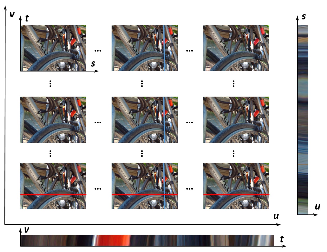
Figure 1: Light field image captured by Lytro Illum with the corresponding horizontal and vertical epipolar plane image.

(a)

(b)

Figure 2: Lenslet image captured by Lytro Illum. (a) Lenslet image; (b) Amplified regions for the red bounding box of (a).

Generally, according to the availability of original reference information, objective IQA algorithms can be classified as full-reference IQA (FR-IQA), reduced-reference IQA (RR-IQA), and no-reference IQA (NR-IQA). Specifically, the FR-IQA methods utilize complete reference image data and measure the difference between reference and distorted images. The RR-IQA models utilize partial information of the reference image for quality assessment, while the NR-IQA metrics evaluate image quality without original reference images, which is more applicable in most real-world scenarios.

(a)

(b)

(c)

(d)

(e)

(f)

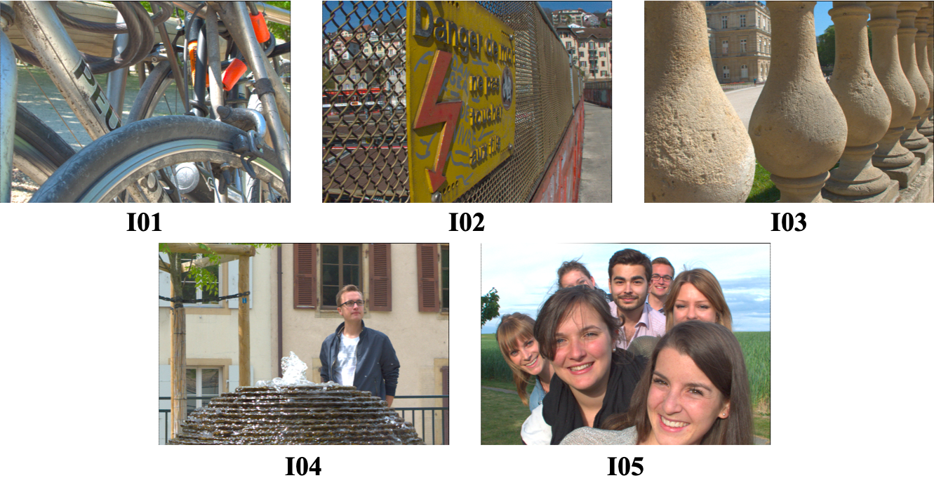
(g)

(h)

Figure 3: (a) Illustration of the center view for the selected image contents of source sequences of Win5-LID; (b) Distribution of Spatial perceptual Information (SI) and Colorfulness (CF) of Win5-LID; (c) Illustration of the center view for the selected image contents of source sequences of MPI-LFA; (d) Distribution of SI and CF of MPI-LFA; (e) Illustration of the center view for the selected image contents of source sequences of SMART; (f) Distribution of SI and CF of SMART; (g) Illustration of the center view for the selected image contents of source sequences of VALID; (h) Distribution of SI and CF of VALID.

For 2D IQA, several 2D FR-IQA metrics have been proposed, for example, structural similarity (SSIM) [18], multi-scale SSIM (MS-SSIM) [19], feature similarity (FSIM) [20], information content weighting SSIM (IWSSIM) [21], internal generative mechanism (IGM) [22], visual saliency-induced index (VSI) [23] and gradient magnitude similarity deviation (GMSD) [24]. The degree of information loss for the distorted image relative to the reference image is evaluated in information fidelity criterion (IFC) [25] and visual information fidelity (VIF) [26]. The noise quality measure (NQM) [27] and visual signal-to-noise ratio (VSNR) [28] consider the human visual system (HVS) sensitivity to different visual signals and the interaction between different signal components. Moreover, there also exist some 2D RR-IQA metrics, such as [29, 30, 31], and 2D NR-IQA metrics. The distortion identification-based image verity and integrity evaluation (DIIVINE) monitors natural image behaviors based on scene statistics [32]. The generalized Gaussian density function is modeled by block discrete cosine transform (DCT) coefficients in blind image integrity notator using DCT statistics (BLIINDS-II) [33]. The blind/referenceless image spatial quality evaluator (BRISQUE) utilizes scene statistics from spatial domain [34]. The natural image quality evaluator (NIQE) extracts image local features and fits a multivariate Gaussian model on the extracted local features [35]. A “bag” of features designed in different color spaces based on human perception are extracted in feature maps-based referenceless image quality evaluation engine (FRIQUEE) [36]. In addition, due to the high dynamic properties of light field content, we also compare with the visual difference predictor for high dynamic range images (HDR-VDP2) [37].

As for 3D IQA, Yang et al. proposed a 3D FR-IQA method based on the average peak signal-to-noise ratio (PSNR) and the absolute difference between left and right views [38]. Chen et al. proposed a 3D FR-IQA algorithm that models the influence of binocular rivalry [39]. They also proposed a 3D NR-IQA algorithm that extracts features from cyclopean images, disparity maps, and uncertainty maps [40]. The S3D integrated quality (SINQ) considers the impact of binocular fusion, rivalry, suppression, and a reverse saliency effect on the distortion perception [41]. The depth information and binocular vision theory are utilized in (BSVQE) [42].

Regarding to multi-view IQA, the morphological pyramid PSNR (MP-PSNR) Full [43] and MP-PSNR Reduc [44] were proposed. Furthermore, morphological wavelet PSNR (MW-PSNR) adopts morphological wavelet decomposition to evaluate multi-view image quality [45]. The 3D synthesized view image quality metric (3DSwIM) is based on the comparison of statistical features extracted from wavelet subbands for original and distorted multi-view images [46]. Gu et al. proposed a NR multi-view IQA metric that employs the autoregression based local image description, which is named as AR-plus thresholding (APT) [47].

However, the above-mentioned algorithms do not take into account the essential characteristics of the LFI. Specifically, the 2D and 3D algorithms ignore the influence of angular consistency, and the multi-view methods cannot effectively measure the deterioration of spatial quality. Therefore, it is important to design an effective light-field-specific metric.

Although there exist the evaluation methods for light field rendering and visualization [48, 49], few objective LFI quality evaluation methods have been proposed. Specifically, Fang et al. proposed a FR LFI-QA method that measures the gradient magnitude similarity of reference and distorted EPIs [50]. The RR LF image quality assessment metric (LF-IQM) assumes that depth map quality is closely related to LFIs overall quality, which measures the structural similarity between original and distorted depth maps to predict the LFI quality [51]. However, neither of these methods utilize texture information of SAI, which causes insufficient measurement of LFI spatial quality. Furthermore, LF-IQM performance is significantly affected by depth estimation algorithms. Additionally, these methods require the use of original LFI information, which limits their application scenarios. Therefore, a general-purpose NR LFI-QA method that fully considers the factors affecting LFI quality is necessary for real applications.

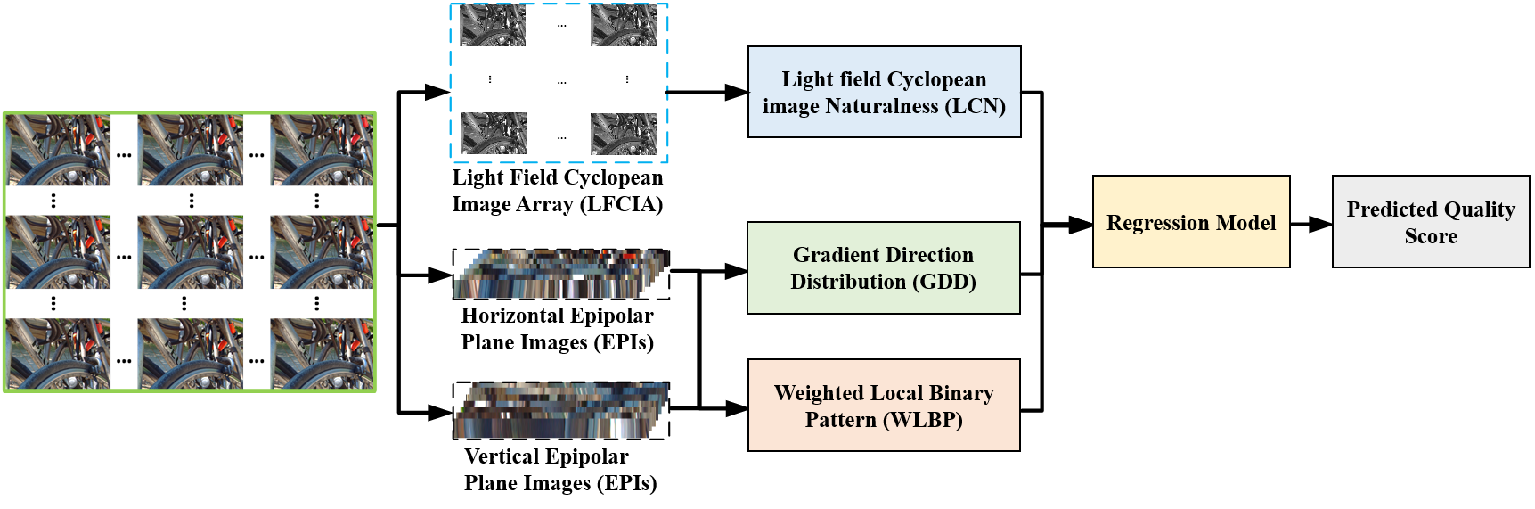
Figure 4: Flow diagram of the proposed No-Reference Light Field image Quality Assessment (NR-LFQA) model.

In this paper, to the best of our knowledge, we propose the first No-Reference Light Field image Quality Assessment (NR-LFQA) scheme. As the LFI can provide the binocular cue and consists of many SAIs [52], we propose Light field Cyclopean image array Naturalness (LCN) to measure the deterioration of spatial quality in LFI, which can take advantage of information from all SAIs and effectively capture the global naturalness distribution of LFI. Specifically, we first mimic binocular fusion and rivalry to generate Light Field Cyclopean Image Array (LFCIA) and then analyze its naturalness distribution. In addition to spatial quality, angular consistency is equally important for the LFI perception [52, 53]. Since the EPI contain angle information of the LFI, we extract features for measuring the degradation of angular consistency on EPI including two key aspects: i) we propose the new Gradient Direction Distribution (GDD) to measure the distribution of EPI gradient direction maps, which can represent the global angular distribution; ii) we then propose the Weighted Local Binary Pattern (WLBP) descriptor to capture the relationship between different SAIs, which focuses on the local angular consistency degradation. Finally, these two features can collectively reflect changes in angular consistency. Our experimental results show that the performance of our proposed NR-LFQA model correlates well with human visual perception and achieves the state-of-the-art performance compared to other objective methods. The software release of NR-LFQA is available online: http://staff.ustc.edu.cn/~chenzhibo/resources.html for public research usage.

The remainder of this paper is organized as follows. Section II introduces adopted datasets in details. In Section IIII, the proposed model is presented. We then illustrate the experimental results in Section IV. Finally, section V concludes our paper.

II Datasets

We conducted experiments on four publicly available datasets, namely Win5-LID [52], MPI-LFA [53], SMART [54] and VALID [55] to examine our proposed NR-LFQA model.

The Win5-LID dataset selects 6 real scenes captured by Lytro illum and 4 synthetic scenes as original images, which cover various Spatial perceptual Information (SI) and Colorfulness (CF) [56], as shown in Fig. 3. The 220 distorted LFIs were produced by 6 distortion types, including HEVC, JPEG2000 (JPEG), linear interpolation (LN), nearest neighbor interpolation (NN) and two CNN models. In addition to CNN models, each distortion includes 5 intensity levels. The observers were asked to rate 220 LFIs under double-stimulus continuous quality scale (DSCQS) on a 5-point discrete scale. The associated overall mean opinion score (MOS) value is provided for each LFI.

As shown in Fig. 3, the MPI-LFA dataset is composed of 14 pristine LFIs captured by the TSC system, covering various SI and CF. Moreover, 336 distorted LFIs were produced based on 6 distortion types (i.e. HEVC, DQ, OPT, LINEAR, NN and GAUSS), with 7 degradation levels for each distortion type. To quantify LFI quality, pair-wise comparison (PC) method with a two-alternative-forced-choice is performed and just-objectionable-differences (JOD) is provided, which is more similar to difference-mean-opinion-score (DMOS). The lower value indicates the worse quality.

The SMART dataset contains 16 original light field images and 256 distorted sequences are obtained by introducing 4 compression distortions (i.e. HEVC intra, JPEG, JPEG2000 and SSDC). The PC method is selected to collect the subjective ratings for each image and the Bradley-Terry (BT) scores are provided. Higher BT score indicates higher preference rate.

The VALID dataset consists of 5 reference LFIs with 140 distorted LFIs spanning 5 compression solutions. The VALID includes both 8bit and 10bit LFIs. The comparison-based adjectival categorical judgement methodology is adopted for 8bit images, while double stimulus impairment scale (DSIS) is performed for 10bit images. Moreover, the MOS values are provided for the LFIs.

III Proposed Method

The block diagram of the proposed model is shown in Fig. 4. First, we analyze the naturalness distribution of LFCIA, which is generated by simulating binocular fusion and binocular rivalry. To measure the degradation of angular consistency, GDD is then computed to analyze the direction distribution of EPI gradient direction maps. The WLBP descriptor is proposed to measure the relationship between different SAIs. Finally, regression model is used to predict LFI quality.

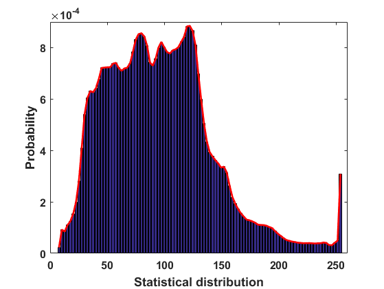
(a)

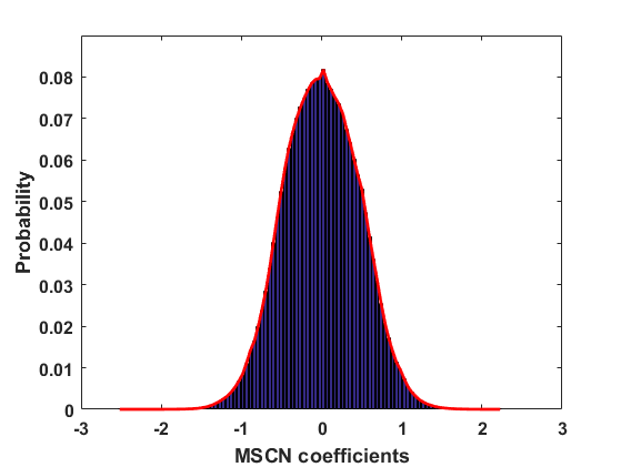
(b)

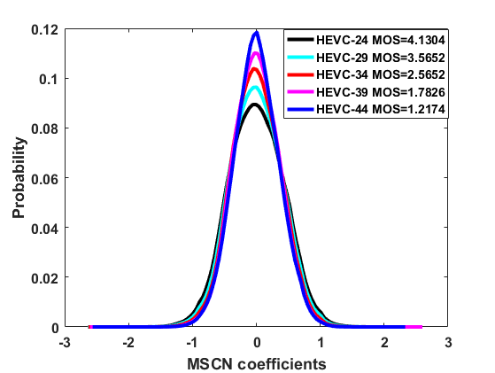
(c)

Figure 5: Statistical distribution of Light Field Cyclopean Image Array (LFCIA) and Mean Subtracted and Contrast Normalized (MSCN) coefficients. (a) Statistical distribution of LFCIA; (b) MSCN coefficients of LFCIA; (c) MSCN coefficients for different HEVC compression levels.

III-A Light field Cyclopean image array Naturalness (LCN)

In general, as the LFI perceptual quality is decided by the HVS, it is reasonable to quantify the LFI quality by characterizing the human perception process. Considering that the LFI can provide binocular perception, we utilize the binocular fusion and binocular rivalry theory to evaluate the spatial quality of LFI. In specific, the disparity between the left and right views of the LFI is small, so most scenes are guaranteed in the comfort zone and binocular fusion occurs [57]. When the perceived contents to the left and right eyes are significantly different, the failures of binocular fusion will lead to binocular rivalry [58].

To simulate the human perception process, the cyclopean perception theory provides us with an executable strategy to achieve this goal [59]. When a stereoscopic image pair is presented, a cyclopean image is formed in the mind of observers. The generated cyclopean image contains both left and right view information and takes into account the impact of binocular fusion and binocular rivalry characteristics, so it can effectively reflect the perceived image quality [39, 41].

Specifically, a cyclopean image is synthesized from the stereoscopic image, disparity map, and spatial activity map. Here, the horizontal adjacent SAIs of the LFI are regraded as a left view and a right view separately. We define the left view as $I_{u,v}(s,t)$, where $(s,t)$ represents the SAI spatial coordinates and $(u,v)\in\{U,V\}$ indicates the angular coordinate of the LFI. The LFCIA with angular resolution of $U\times(V-1)$ can be synthesized by the following model:

$$C_{u,v}(s,t)=W_{u,v}(s,t)\times I_{u,v}(s,t)+$$ (1)

$$W_{u+1,v}(s,t)\times I_{u+1,v}((s,t)+d_{s,t}),$$

where $C_{u,v}$ represents a sub-cyclopean image at angular coordinate $(u,v)$ and $d_{s,t}$ is the horizontal disparity between $I_{u,v}$ and $I_{u+1,v}$ at spatial coordinate $(s,t)$. The disparity map $d$ is generated by using a simple stereo disparity estimation algorithm, which utilizes the SSIM index as a matching criterion [39]. The weights $W_{u,v}$ and $W_{u+1,v}$ are computed by the following formulas:

$$W_{u,v}(s,t)=\frac{\varepsilon[S_{u,v}(s,t)]+A_{1}}{\varepsilon[S_{u,v}(s,t)]+\varepsilon[S_{u+1,v}((s,t)+d_{s,t})]+A_{1}},$$ (2)

$$W_{u+1,v}(s,t)=\frac{\varepsilon[S_{u+1,v}((s,t)+d_{s,t})]+A_{1}}{\varepsilon[S_{u,v}(s,t)]+\varepsilon[S_{u,v+1}((s,t)+d_{s,t})]+A_{1}},$$ (3)

where $A_{1}$ is the small value to guarantee stability. $S_{u,v}(s,t)$ is $N\times N$ region pixels centered on $(s,t)$ and $\varepsilon[S_{u,v}(s,t)]$ is the spatial activity within $S_{u,v}(s,t)$. We then obtain the spatial activity map as follows:

$$\varepsilon[S_{u,v}(s,t)]=\log_{2}[var_{u,v}^{2}(s,t)+A_{2}],$$ (4)

where $var_{u,v}(s,t)$ is the variance of $S_{u,v}(s,t)$ and unit item $A_{2}$ guarantee the activity is positive. Similarly, we define quantities $S_{u+1,v}(s,t)$, $var_{u+1,v}(s,t)$ and $\varepsilon[S_{u+1,v}(s,t)]$ on the $I_{u+1,v}(s,t)$.

After obtaining the LFCIA, the locally Mean Subtracted and Contrast Normalized (MSCN) coefficients are utilized to measure their naturalness, which have been successfully employed for image processing tasks and can be used to model the contrast-gain masking process in early human vision [34, 60]. For each sub-cyclopean image, its MSCN coefficients can be calculated by:

$$\widehat{C}_{u,v}(s,t)=\frac{C_{u,v}(s,t)-\mu_{u,v}(s,t)}{\sigma_{u,v}(s,t)+1},$$ (5)

where $\widehat{C}_{u,v}(s,t)$ and $C_{u,v}(s,t)$ represent the MSCN coefficients image and sub-cyclopean image values at spatial position $(s,t)$ respectively. $\mu_{u,v}(s,t)$ and $\sigma_{u,v}(s,t)$ stands for the local mean and standard deviation in a local patch centered at $(s,t)$. They are respectively calculated as:

$$\mu_{u,v}(s,t)=\sum\limits_{k=-K}^{K}\sum\limits_{l=-L}^{L}z_{k,l}C_{u,v}^{k,l}(s,t),$$ (6)

$$\sigma_{u,v}(s,t)=\sqrt{\sum\limits_{k=-K}^{K}\sum\limits_{l=-L}^{L}z_{k,l}(C_{u,v}^{k,l}(s,t)-\mu_{u,v}(s,t))^{2}},$$ (7)

where $z=\{z_{k,l}|k=-K,...,K,l=-L,...,L\}$ denotes a 2D circularly-symmetric gaussian weighting function sampled out 3 standard deviations and rescaled to unit volume. We set $K=L=3$ in our implement.

To measure the spatial quality of the LFI, we consider the naturalness distribution of LFCIA. In specific, the MSCN coefficients of all sub-cyclopean images are superimposed. As shown in Fig. 5(a) and Fig. 5(b), the distribution of MSCN coefficients is significantly different from the statistical distribution of sub-cyclopean images and approximates the Gaussian distribution. Fig. 5(c) illustrates the MSCN coefficients distributions of LFIs with different high efficiency video coding (HEVC) compression levels, the results of which represent that the MSCN coefficients distributions are very indicative when the LFI suffer from distortions. Here the sample of LFI is selected from the Win5-LID dataset [52]. Then, we utilize the zero-mean asymmetric generalized gaussian distribution (AGGD) model to qualify MSCN coefficients distribution, which can fit the distribution by:

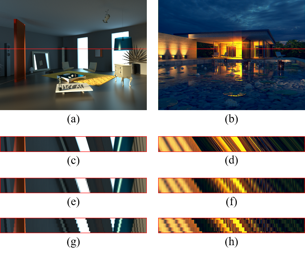
Figure 6: Horizontal EPI for a undistorted LFI and its various distorted versions. The samples are selected from the MPI-LFI dataset [53]. (a-b) Center view of the LFIs and the red line indicates the row position at which the EPI is acquired; (c-d) Original EPIs; (e-f) Distorted EPIs with LINEAR distortion; (g-h) Distorted EPIs with NN distortion.

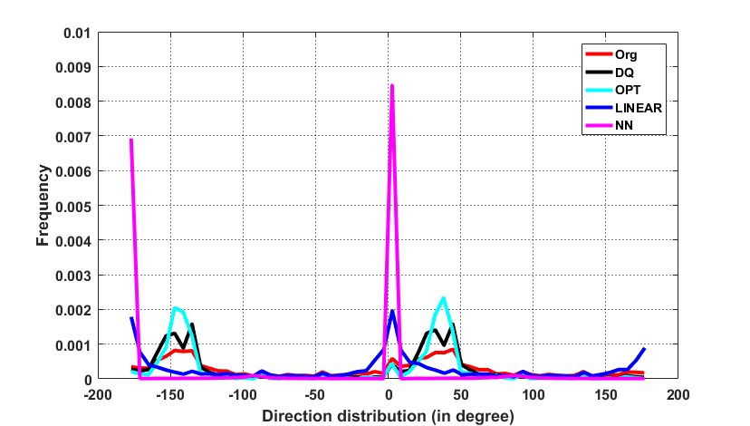
Figure 7: Gradient direction distribution for a undistorted LFI and its various distorted types.

$$f(x;\alpha,\sigma_{l}^{2},\sigma_{r}^{2})=\left\{\begin{aligned} \frac{\alpha}{(\beta_{l}+\beta_{r})\Gamma(\frac{1}{\alpha})}exp(-(\frac{-x}{\beta_{l}})^{\alpha})&&x<0\\ \frac{\alpha}{(\beta_{l}+\beta_{r})\Gamma(\frac{1}{\alpha})}exp(-(\frac{-x}{\beta_{r}})^{\alpha})&&x\geqslant 0,\end{aligned}\right.$$ (8)

where

$$\beta_{l}=\sigma_{l}\sqrt{\frac{\Gamma(\frac{1}{\alpha})}{\Gamma(\frac{3}{\alpha})}}\quad and\quad\beta_{r}=\sigma_{r}\sqrt{\frac{\Gamma(\frac{1}{\alpha})}{\Gamma(\frac{3}{\alpha})}},$$ (9)

and $\alpha$ is the shape parameter controlling the shape of the statistic distribution, while $\sigma_{l}$, $\sigma_{r}$ are the scale parameters of the left and right sides respectively. If $\sigma_{l}=\sigma_{r}$, AGGD can become generalized gaussian distribution (GGD) model. In addition, we utilize aforementioned three parameters to compute $\eta$ as another feature:

$$\eta=(\beta_{r}-\beta_{l})\frac{\Gamma(\frac{2}{\alpha})}{\Gamma(\frac{1}{\alpha})}.$$ (10)

We further compute kurtosis and skewness as supplementary features. In addition, the SAIs are downsampled by a factor of 2, which has been proven to improve the correlation between model prediction and subjective assessment [34]. Finally, LFCIA naturalness $F_{LCN}$ is obtained.

III-B Global Direction Distribution (GDD)

(a)

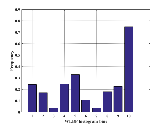
(b)

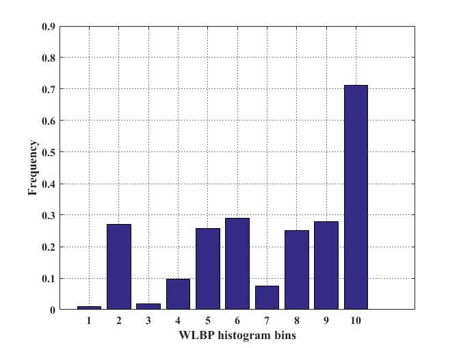
(c)

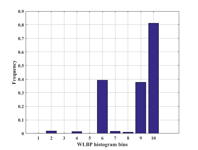
(d)

Figure 8: Illustration of the statistical distribution of WLBP with different distortion types from MPI-LFA [53]. Here we set $R=1$ and $P=8$. (a) Quantized depth maps (DQ). (b) Optical flow estimation (OPT). (c) LINEAR interpolation. (d) Nearest Neighbor (NN) interpolation.

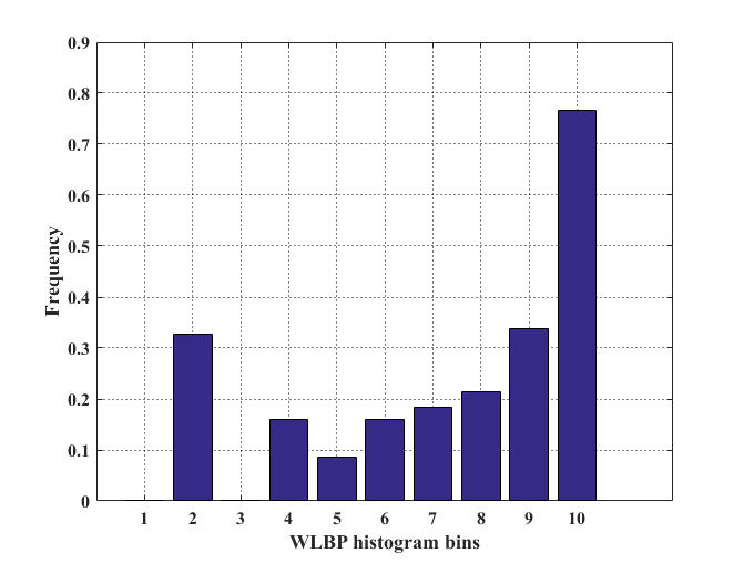
(a)

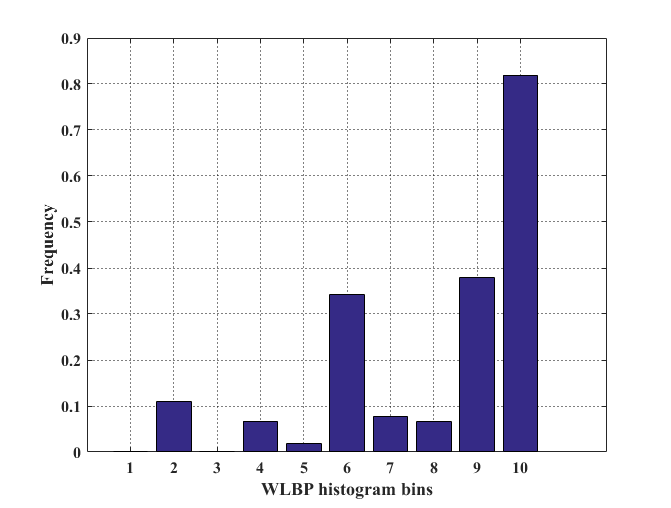
(b)

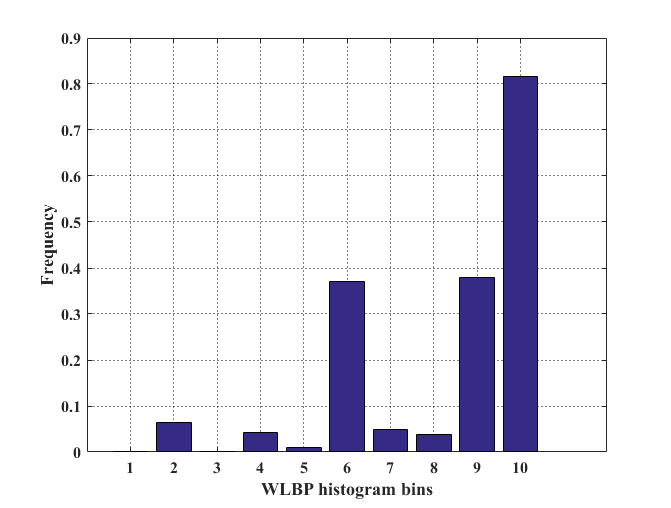
(c)

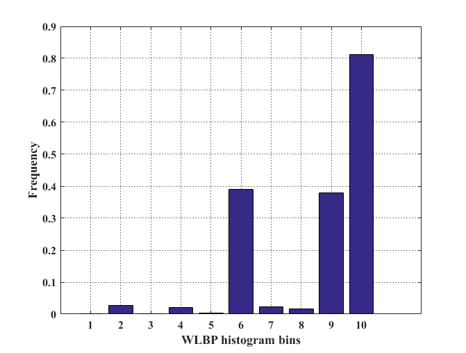
(d)

Figure 9: Illustration of the statistical distribution of WLBP with different NN distortion levels from MPI-LFA [53]. Here we set $R=1$ and $P=8$. (a) Level 1; (b) Level 2; (c) Level 3; (d) Level 4.

The LFI quality is affected by spatial quality and angular consistency. Usually, angular reconstruction operations, such as interpolation, will break angular consistency. To measure the deterioration of angular consistency, extracting features from the EPI is an executable strategy because it contains the angular information of the LFI.

Traditionally, the slopes of lines in the EPI reflect the depth of the scene captured by light field. Many LFI processing tasks, such as super resolution and depth map estimation, benefit from this particular property [3, 61]. As shown in Fig. 6(c-d), the slopes of lines in the undistorted EPI can effectively reflect the depth and disparity information in Fig. 6(a-b). Here the LFIs are from MPI-LFA dataset [53].

However, angular distortion damages existing structures and significantly changes the distribution of the slopes of lines in the EPI, as presented in Fig. 6(e-h). Specifically, we find that the distorted EPIs with the same distortion type have a similar distribution, indicating that the angular distortion is not sensitive to the depth and content of the original LFI. Therefore, the slopes of lines in distorted EPI can be utilized to capture the degradation of angular distortion of LFI.

To extract the Gradient Direction Distribution (GDD) features, we first compute the gradient direction maps of EPIs and then analyze the distribution of the gradient direction maps to obtain the features. We define the vertical EPI and horizontal EPI as $E_{u^{*},s^{*}}(v,t)$ and $E_{v^{*},t^{*}}(u,s)$ respectively, where $u^{*},s^{*}$ and $v^{*},t^{*}$ represent the fixed coordinates. Then we analyze the direction distribution of EPI by calculating the gradient direction maps of EPI:

$$G_{u^{*},s^{*}}=atan2(-Ey_{u^{*},s^{*}},Ex_{u^{*},s^{*}})*\frac{180}{\pi},$$ (11)

where

$$Ex_{u^{*},s^{*}}=E_{u^{*},s^{*}}\otimes h_{x}\quad and\quad Ey_{u^{*},s^{*}}=E_{u^{*},s^{*}}\otimes h_{y},$$ (12)

$$h_{x}={\left[\begin{array}[]{ccc}-1&0&1\\ -2&0&2\\ -1&0&1\end{array}\right]},\quad h_{y}={\left[\begin{array}[]{ccc}-1&-2&-1\\ 0&0&0\\ 1&2&1\end{array}\right]}.$$ (13)

Similar to the computation process of $G_{u^{*},s^{*}}$, we can obtain the gradient direction maps $G_{v^{*},t^{*}}$ of horizontal EPI. We then quantify the gradient direction maps to 360 bins, i.e. from $-180^{\circ}$ to $179^{\circ}$. As shown in Fig. 7, various distortion types exert systematically different influences on the EPIs. It can be seen that the original EPI has a direction histogram concentrated on about $-150^{\circ}$ and $30^{\circ}$, while the distorted EPIs manifest different distributions. Specifically, the nearest neighbor (NN) and LINEAR interpolation distortions make the EPIs appear stepped, and their direction is mainly concentrated at $-180^{\circ}$ and $0^{\circ}$. The optical flow estimation (OPT) and quantized depth maps (DQ) distortions show higher peaks at $-150^{\circ}$ and $30^{\circ}$. Overall, gradient direction distribution is effective for measuring the degradation of angular consistency.

Finally, we calculate the mean value, entropy, skewness and kurtosis of the $G_{u^{*},s^{*}}$ and $G_{v^{*},t^{*}}$, respectively. Since the LFI contains many EPIs, we average the mean value, entropy, skewness and kurtosis of all EPIs to obtain the feature $F_{GDD}$.

III-C Weighted Local Binary Pattern (WLBP)

TABLE I: Performance Comparison on Win5-LID, MPI-LFA, and SMART Datasets.

		Win5-LID				MPI-LFA				SMART
Type	Metrics	SRCC	LCC	RMSE	OR	SRCC	LCC	RMSE	OR	SRCC	LCC	RMSE	OR
2D FR	PSNR	0.6026	0.6189	0.8031	0.0045	0.8078	0.7830	1.2697	0.0060	0.7045	0.7035	1.5330	0.0195
	SSIM [18]	0.7346	0.7596	0.6650	0.0000	0.7027	0.7123	1.4327	0.0060	0.6862	0.7455	1.4378	0.0156
	MS-SSIM [19]	0.8266	0.8388	0.5566	0.0000	0.7675	0.7518	1.3461	0.0060	0.6906	0.7539	1.4171	0.0117
	FSIM [20]	0.8233	0.8318	0.5675	0.0045	0.7776	0.7679	1.3075	0.0030	0.7811	0.8139	1.2533	0.0039
	IWSSIM [21]	0.8352	0.8435	0.5492	0.0000	0.8124	0.7966	1.2340	0.0030	0.7111	0.7971	1.3024	0.0000
	IFC [25]	0.5028	0.5393	0.8611	0.0000	0.7573	0.7445	1.3629	0.0030	0.4827	0.5946	1.7343	0.0156
	VIF [26]	0.6665	0.7032	0.7270	0.0000	0.7843	0.7861	1.2618	0.0030	0.0684	0.2533	2.0867	0.0469
	NQM [27]	0.6508	0.6940	0.7362	0.0045	0.7202	0.7361	1.3817	0.0060	0.4601	0.5305	1.8285	0.0234
	VSNR [28]	0.3961	0.5050	0.8826	0.0182	0.7427	0.5787	1.6651	0.0179	0.5542	0.6289	1.6770	0.0156
	HDR-VDP2 [37]	0.5555	0.6300	0.7941	0.0045	0.8608	0.8385	1.1123	0.0000	0.1888	0.3347	2.0327	0.0625
2D NR	BRISQUE [34]	0.6687	0.7510	0.5619	0.0000	0.6724	0.7597	1.1317	0.0000	0.8239	0.8843	0.8325	0.0000
	NIQE [35]	0.2086	0.2645	0.9861	0.0045	0.0665	0.1950	2.0022	0.0327	0.1386	0.1114	2.1436	0.0547
	FRIQUEE [36]	0.6328	0.7213	0.5767	0.0000	0.6454	0.7451	1.1036	0.0000	0.7269	0.8345	0.9742	0.0000
3D FR	Chen [39]	0.5269	0.6070	0.8126	0.0091	0.7668	0.7585	1.3303	0.0030	0.6798	0.7722	1.3706	0.0078
3D NR	SINQ [41]	0.8029	0.8362	0.5124	0.0000	0.8524	0.8612	0.9939	0.0000	0.8682	0.8968	0.9653	0.0000
	BSVQE [42]	0.8179	0.8425	0.4801	0.0000	0.8570	0.8751	0.9561	0.0000	0.8449	0.8992	0.8514	0.0000
Multi-view FR	MP-PSNR Full [43]	0.5335	0.4766	0.8989	0.0000	0.7203	0.6730	1.5099	0.0089	0.8449	0.8992	0.8514	0.0000
	MP-PSNR Reduc [44]	0.5374	0.4765	0.8989	0.0000	0.7210	0.6747	1.5067	0.0089	0.6716	0.6926	1.5559	0.0117
	MW-PSNR Full [45]	0.5147	0.4758	0.8993	0.0000	0.7232	0.6770	1.5023	0.0089	0.6620	0.6505	1.6382	0.0117
	MW-PSNR Reduc [45]	0.5326	0.4766	0.8989	0.0000	0.7217	0.6757	1.5048	0.0089	0.6769	0.6903	1.5607	0.0117
	3DSwIM [46]	0.4320	0.5262	0.8695	0.0182	0.5565	0.5489	1.7063	0.0119	0.4053	0.4707	1.9032	0.0234
Multi-view NR	APT [47]	0.3058	0.4087	0.9332	0.0045	0.0710	0.0031	2.0413	0.0357	0.5105	0.5249	1.8361	0.0234
LFI FR	Fang [50]	-	-	-	-	0.7942	0.8065	1.2300	-	-	-	-	-
LFI RR	LF-IQM [51]	0.4478	0.5193	0.8584	0.0227	0.3334	0.4360	1.8038	0.0149	0.1701	0.2101	1.0279	0.0392
LFI NR	Proposed NR-LFQA	0.9032	0.9206	0.3876	0.0000	0.9119	0.9155	0.7556	0.0000	0.8803	0.9105	0.8300	0.0000

TABLE II: Performance Comparison on VALID Dataset.

		VALID-8bit				VALID-10bit
Type	Metrics	SRCC	LCC	RMSE	OR	SRCC	LCC	RMSE	OR
2D FR	PSNR	0.9620	0.9681	0.3352	0.0000	0.9467	0.9524	0.2935	0.0000
	SSIM [18]	0.9576	0.9573	0.3868	0.0000	0.9326	0.9375	0.3348	0.0000
	MS-SSIM [19]	0.9593	0.9658	0.3473	0.0000	0.9432	0.9484	0.3051	0.0000
	FSIM [20]	0.9695	0.9798	0.2678	0.0000	-	-	-	-
	IWSSIM [21]	0.9674	0.9764	0.2892	0.0000	0.9499	0.9617	0.2638	0.0000
	IFC [25]	0.9693	0.9909	0.1800	0.0000	-	-	-	-
	VIF [26]	0.9749	0.9870	0.2150	0.0000	-	-	-	-
	NQM [27]	0.9055	0.9194	0.5266	0.0000	0.8410	0.8582	0.4940	0.0000
	VSNR [28]	0.9359	0.9324	0.4838	0.0000	-	-	-	-
	HDR-VDP2 [37]	0.9623	0.9785	0.2758	0.0000	0.9371	0.9528	0.2921	0.0000
2D NR	BRISQUE [34]	0.9222	0.9849	0.2017	0.0000	0.9027	0.9347	0.2838	0.0000
	NIQE [35]	0.8636	0.9524	0.4080	0.0000	-	-	-	-
	FRIQUEE [36]	0.9157	0.9836	0.2160	0.0000	0.8559	0.8986	0.3497	0.0000
3D FR	Chen [39]	0.9642	0.9738	0.3046	0.0000	-	-	-	-
3D NR	SINQ [41]	0.9222	0.9849	0.2070	0.0000	0.9021	0.9348	0.2722	0.0000
	BSVQE [42]	0.9222	0.9814	0.2180	0.0000	-	-	-	-
Multi-view FR	MP-PSNR Full [43]	0.9730	0.9852	0.2291	0.0000	0.3830	0.3582	0.8986	0.0000
	MP-PSNR Reduc [44]	0.9744	0.9859	0.2237	0.0000	0.3826	0.3506	0.9013	0.0000
	MW-PSNR Full [45]	0.9597	0.9677	0.3376	0.0000	0.3764	0.3556	0.8995	0.0000
	MW-PSNR Reduc [45]	0.9648	0.9751	0.2970	0.0000	0.3815	0.3563	0.8993	0.0100
	3DSwIM [46]	0.7950	0.7876	0.8248	0.0000	0.7869	0.7401	0.6472	0.0000
Multi-view NR	APT [47]	0.4699	0.6452	1.0228	0.0000	-	-	-	-
LFI RR	LF-IQM [51]	0.3571	0.4708	1.0712	0.0000	0.3692	0.4828	0.8137	0.0000
LFI NR	Proposed NR-LFQA	0.9286	0.9799	0.2380	0.0000	0.9228	0.9517	0.2769	0.0000

Since the pixels in each row of the EPI come from different SAIs, the relationship between the pixels of each row can reflect the relationship of the SAIs. This property indicates that we can analyze the relative relationship of pixels in EPI to measure the change in angular consistency. In addtion, measuring the relationship between pixels at different distances can capture local angular consistency information.

(a)

(b)

(c)

(d)

(e)

Figure 10: The scatter plots of predicted quality scores by different methods against the MOS values on the Win5-LID. The horizontal axis in each figure denotes predicted quality scores and the vertical axis in each figure represents the MOS values. The red line is the fitted curve. (a) FSIM; (b) MS-SSIM; (c) IWSSIM; (d) BSVQE; (e) Proposed.

As a result, we propose Weighted Local Binary Pattern (WLBP) to capture the relationship between different SAIs. The LBP is able to extract local distribution information, which has proven its effectiveness in many works and has shown good performance for the evaluation of 2D-IQA tasks [62, 63, 64, 65, 66, 67]. We first calculate the local rotation invariant uniform LBP operator $L_{u^{*},s^{*}}^{R,P}$ of the vertical EPI $E_{u^{*},s^{*}}$ by:

$$L_{u^{*},s^{*}}^{R,P}(E_{u^{*},s^{*}}^{c})=\left\{\begin{aligned} \sum_{p=0}^{P-1}\theta(E_{u^{*},s^{*}}^{p}-E_{u^{*},s^{*}}^{c})&&\psi(\hat{L}_{u^{*},s^{*}}^{R,P})\leq 2\\ P+1&&otherwise,\end{aligned}\right.$$ (14)

where $R$ is the radius value and $P$ indicates the number of neighboring points. $E_{u^{*},s^{*}}^{c}$ represents a center pixel at the position $(x_{c},y_{c})$ in the corresponding EPIs and $E_{u^{*},s^{*}}^{p}$ is a neighboring pixel $(x_{p},y_{p})$ surrounding $E_{u^{*},s^{*}}^{c}$:

$$x_{p}=x_{c}+R\cos(2\pi\frac{p}{P})\quad and\quad y_{p}=y_{c}-R\sin(2\pi\frac{p}{P}),$$ (15)

where $p\in\{1,2...P\}$ is the number of neighboring pixels sampled by a distance $R$ from $E_{u^{*},s^{*}}^{c}$ to $E_{u^{*},s^{*}}^{p}$. In this case, $\theta(z)$ is the step function and defined by:

$$\theta(z)=\left\{\begin{aligned} 1&&z\geqslant T\\ 0&&otherwise,\end{aligned}\right.$$ (16)

where $T$ indicates the threshold value. In addition, $\psi$ is used to compute the number of bitwise transitions:

$$\psi(L_{u^{*},s^{*}}^{R,P})=||\theta(E_{u^{*},s^{*}}^{P-1}-E_{u^{*},s^{*}}^{c})-\theta(E_{u^{*},s^{*}}^{0}-E_{u^{*},s^{*}}^{c})||$$ (17)

$$+\sum_{p=1}^{P-1}||\theta(E_{u^{*},s^{*}}^{p}-E_{u^{*},s^{*}}^{c})-\theta(E_{u^{*},s^{*}}^{p-1}-E_{u^{*},s^{*}}^{c})||,$$

and $\hat{L}_{u^{*},s^{*}}^{R,P}$ is rotation-invariant operator:

$$\hat{L}_{u^{*},s^{*}}^{R,P}(E_{u^{*},s^{*}}^{c})=min\{ROR(\sum\limits_{p=0}^{P-1}\theta(E_{u^{*},s^{*}}^{p}-E_{u^{*},s^{*}}^{c})2^{p},k)\},$$ (18)

where $k\in\{0,1,2...,P-1\}$ and $ROR(\beta,k)$ is the circular bit-wise right shift operator that shifts the tuple $\beta$ by $k$ positions. Finally, we obtain $L_{u^{*},s^{*}}^{R,P}$ with a length of $P+2$.

(a)

(b)

Figure 11: Box plot of SRCC distributions of algorithms over 1000 trials. (a) On Win5-LID dataset; (b) On MPI-LFA dataset.

For a LFI, there exist many EPIs in the vertical and horizontal directions. If we concatenate the LBP features that extracted from each EPI, it will induce a dimensional disaster. To reduce the feature dimension, entropy weighting is adopted because some EPIs have little information and their LBP features are mainly concentrated in one statistical direction. This represents that these EPIs contain less angular consistency information and their entropy values are close to zero. Therefore, we can obtain the WLBP of vertical EPI $E_{u^{*},s^{*}}$ as follows:

$$Lver_{R,P}=\frac{\sum\limits_{u=1}^{U}\sum\limits_{s=1}^{S}w_{u,s}^{R,P}.*L_{u,s}^{R,P}}{\sum\limits_{u=1}^{U}\sum\limits_{s=1}^{S}w_{u,s}^{R,P}},$$ (19)

where the entropy of $L_{u,s}^{R,P}$ is computed as weight $w_{u,s}^{R,P}$. At the same time, we adopt the same operation to obtain the WLBP features $Lhor_{R,P}$ of the horizontal EPI $E_{v^{*},t^{*}}$.

In our implement, we set $R\in\{1,2,3\}$, $P=3\times R$ and $T=R/2$. Finally, we combine all features to obtain feature $F_{WLBP}$ as follows:

$$F_{WLBP}=\{Lver_{R,P},Lhor_{R,P}\}.$$ (20)

Fig. 8 illustrates the WLBP histogram of various distortion types with $R=1$ and $P=8$. The LFIs are selected from MPI-LFA dataset [53]. Specifically, the WLBP features are extracted from horizontal and vertical EPIs separately. For MPI-LFA dataset, the LFIs only contain horizontal EPIs. Moreover, for the WLBP feature with parameter $(R,P)$, we can generate $P+2$ histogram bins [62]. Therefore, when $P=8$, the corresponding feature dimension is $P+2=10$. Furthermore, the histogram of WLBP for NN distortion with different distortion levels for $R=1$ and $P=8$ is shown in Fig. 9. As the figures show that there is a significant difference in the WLBP distribution for different distortion types, and the WLBP distribution changes significantly as the distortion level increases. Overall, WLBP can effectively capture the characteristics of local angular consistency degradation in EPI.

III-D Quality Evaluation

In order to conduct the quality assessment, we train a regression model to map the final feature vector $F_{Final}=\{F_{LCN},F_{GDD},F_{WLBP}\}$ space to quality scores. In our implementation, we utilize support vector regression (SVR) model, which can automatically learn the weights of these features from the data distribution. In other words, the weights of these proposed features are different. Moreover, the SVR model has been applied to many image quality assessment problems [68, 42, 41] and has demonstrated its effectiveness The LIBSVM package [69] is exploited to implement the SVR with a radial basis function (RBF) kernel.

TABLE III: Performance Comparison Between Row and Column Methods With T-test on Win5-LID Dataset. The Symbol ‘1’, ‘0’, or ‘-1’ Represents that the Row Method is Statistically Better, Indistinguishable, or Worse Than The Column Algorithm. Due to Space Constraints, Here We Use the Referenced Number Instead of The Algorithm Name.

	PSNR	[18]	[26]	[20]	[19]	[21]	[28]	[25]	[27]	[35]	[34]	[36]	[39]	[41]	[42]	[46]	[45]	[45]	[44]	[43]	[47]	[51]	Proposed
PSNR	0	-1	-1	-1	-1	-1	1	1	-1	1	-1	-1	1	-1	-1	1	1	1	1	1	1	1	-1
[18]	1	0	1	-1	-1	-1	1	1	1	1	1	1	1	-1	-1	1	1	1	1	1	1	1	-1
[26]	1	-1	0	-1	-1	-1	1	1	1	1	0	1	1	-1	-1	1	1	1	1	1	1	1	-1
[20]	1	1	1	0	0	-1	1	1	1	1	1	1	1	1	0	1	1	1	1	1	1	1	-1
[19]	1	1	1	0	0	-1	1	1	1	1	1	1	1	1	1	1	1	1	1	1	1	1	-1
[21]	1	1	1	1	1	0	1	1	1	1	1	1	1	1	1	1	1	1	1	1	1	1	-1
[28]	-1	-1	-1	-1	-1	-1	0	-1	-1	1	-1	-1	-1	-1	-1	-1	-1	-1	-1	-1	1	-1	-1
[25]	-1	-1	-1	-1	-1	-1	1	0	-1	1	-1	-1	-1	-1	-1	1	-1	-1	-1	-1	1	1	-1
[27]	1	-1	-1	-1	-1	-1	1	1	0	1	-1	1	1	-1	-1	1	1	1	1	1	1	1	-1
[35]	-1	-1	-1	-1	-1	-1	-1	-1	-1	0	-1	-1	-1	-1	-1	-1	-1	-1	-1	-1	-1	-1	-1
[34]	1	-1	0	-1	-1	-1	1	1	1	1	0	1	1	-1	-1	1	1	1	1	1	1	1	-1
[36]	1	-1	-1	-1	-1	-1	1	1	-1	1	-1	0	1	-1	-1	1	1	1	1	1	1	1	-1
[39]	-1	-1	-1	-1	-1	-1	1	1	-1	1	-1	-1	0	-1	-1	1	0	1	-1	0	1	1	-1
[46]	1	1	1	-1	-1	-1	1	1	1	1	1	1	1	0	-1	1	1	1	1	1	1	1	-1
[42]	1	1	1	0	-1	-1	1	1	1	1	1	1	1	1	0	1	1	1	1	1	1	1	-1
[46]	-1	-1	-1	-1	-1	-1	1	-1	-1	1	-1	-1	-1	-1	-1	0	-1	-1	-1	-1	1	-1	-1
[45]	-1	-1	-1	-1	-1	-1	1	1	-1	1	-1	-1	0	-1	-1	1	0	1	0	0	1	1	-1
[45]	-1	-1	-1	-1	-1	-1	1	1	-1	1	-1	-1	-1	-1	-1	1	-1	0	-1	-1	1	1	-1
[44]	-1	-1	-1	-1	-1	-1	1	1	-1	1	-1	-1	1	-1	-1	1	0	1	0	0	1	1	-1
[43]	-1	-1	-1	-1	-1	-1	1	1	-1	1	-1	-1	0	-1	-1	1	0	1	0	0	1	1	-1
[47]	-1	-1	-1	-1	-1	-1	-1	-1	-1	1	-1	-1	-1	-1	-1	-1	-1	-1	-1	-1	0	-1	-1
[51]	-1	-1	-1	-1	-1	-1	1	-1	-1	1	-1	-1	-1	-1	-1	1	-1	-1	-1	-1	1	0	-1
Proposed	1	1	1	1	1	1	1	1	1	1	1	1	1	1	1	1	1	1	1	1	1	1	0

We select four evaluation criteria to measure the performance of objective quality assessment models, namely Spearman rank-order correlation coefficient (SRCC), linear correlation coefficient (LCC), root-mean-square-error (RMSE) and outlier ratio (OR). The SRCC measures the monotonicity, while the LCC evaluates the linear relationship between predict scores and MOS values. The RMSE and OR measure the prediction accuracy and prediction consistency, respectively. The SRCC and LCC values closing to 1 represent high positive correlation and a lower RMSE/OR value indicates a better performance. Additionally, each dataset is randomly divided into 80% for training and 20% for testing. We perform 1000 iterations of cross validation on each dataset, and provide the median SRCC, LCC, RMSE and OR performance as the final measurement. Before computing the LCC, RMSE and OR, a non-linear function is employed by:

$$q^{\prime}=\beta_{1}\{\frac{1}{2}-\frac{1}{1+exp[\beta_{2}(q-\beta_{3})]}\}+\beta_{4}q+\beta_{5},$$ (21)

where $q$ is the output of a method. The parameters $\beta_{1\cdots 5}$ are optimized to minimize a given goodness-of-fit measure. Although the prediction range of the model is different, all prediction scores can be guaranteed to be evaluated on the same scale after logistic function fitting.

TABLE IV: Performance Comparison of Existing Algorithms on EPIs.

	Win5-LID			MPI-LFA
Metrics	SRCC	LCC	RMSE	SRCC	LCC	RMSE
PSNR	0.7190	0.7213	0.7083	0.7198	0.6972	1.4634
FSIM [20]	0.7545	0.7780	0.6424	0.7920	0.7818	1.2730
IFC [25]	0.5323	0.5010	0.8850	0.7265	0.7394	1.3743
BRISQUE [34]	0.7727	0.8473	0.4890	0.7864	0.7850	1.0453
FRIQUEE [36]	0.6225	0.6648	0.5784	0.7523	0.7652	1.0753
Fang [50]	-	-	-	0.7942	0.8065	1.2300
Proposed	0.8829	0.9015	0.3993	0.8905	0.8954	0.8259

TABLE V: Performance of Three Quality Components on Win5-LID and MPI-LFA Datasets.

	Win5-LID			MPI-LFA
Features	SRCC	LCC	RMSE	SRCC	LCC	RMSE
$F_{LCN}$	0.7464	0.8370	0.5128	0.5806	0.6260	1.2891
$F_{GDD}$	0.7431	0.7745	0.6090	0.5621	0.6205	1.1383
$F_{WLBP}$	0.8528	0.8771	0.4006	0.8437	0.8573	0.8900

For OR computation, according to [70, 71, 72], we calculate the standard deviation of the testing set. If the difference between the predicted score and the subjective score is more than 2 times the standard deviation, this can be defined as the outlier. Specifically, the OR represents the mapped objective scores deviating from the subjective ratings in 2 standard deviation as:

$$OR=\frac{\sum\limits_{i=1}^{N}{(|{{s}_{i}}-{{f}_{i}}|>2{{\sigma}_{i}})}}{N},$$ (22)

where $N$ is the size of the testing set. ${s}_{i}$ and ${f}_{i}$ denote the $i$-th subjective score and the $i$-th mapped objective score after the non-linear mapping, respectively. ${\sigma}_{i}$ is the $i$-th standard deviation of the subjective scores.

III-E Comparison with Other Objective Metrics

TABLE VI: SRCC of Different Distortion Types on Win5-LID and MPI-LFA Datasets.

		Win5-LID				MPI-LFA
Type	Metrics	HEVC	JPEG	LN	NN	HEVC	DQ	OPT	Linear	NN	GAUSS
2D FR	PSNR	0.8183	0.8302	0.8135	0.8734	0.9226	0.7664	0.6842	0.9090	0.8895	0.9239
	SSIM [18]	0.9351	0.8390	0.8501	0.8226	0.9769	0.4468	0.5609	0.8055	0.7682	0.9800
	MS-SSIM [19]	0.9731	0.8947	0.8789	0.8346	0.9791	0.7087	0.6556	0.8763	0.8775	0.9702
	FSIM [20]	0.9756	0.9006	0.8876	0.8661	0.9844	0.7631	0.6969	0.8745	0.8704	0.9502
	IWSSIM [21]	0.9690	0.9046	0.8851	0.8313	0.9831	0.7628	0.7336	0.9144	0.9256	0.9662
	IFC [25]	0.8634	0.7299	0.6179	0.8037	0.9430	0.8462	0.7909	0.9147	0.9261	0.8852
	VIF [26]	0.9627	0.8982	0.8287	0.8816	0.9818	0.7057	0.6445	0.9163	0.9048	0.9506
	NQM [27]	0.8861	0.7878	0.7086	0.7214	0.9515	0.6598	0.5596	0.8444	0.9264	0.9333
	VSNR [28]	0.9162	0.8861	0.0208	0.1705	0.9871	0.6082	0.6634	0.8333	0.8256	0.9462
	HDR-VDP2 [37]	0.7322	0.5282	0.7912	0.8711	0.8065	0.7448	0.7953	0.8632	0.9008	0.9309
2D NR	BRISQUE [34]	0.9152	0.9394	0.8268	0.2516	0.9429	0.6121	0.7059	0.7333	0.0941	0.8286
	NIQE [35]	0.1332	0.2161	0.3749	0.1514	0.9186	0.0500	0.1226	0.2616	0.1457	0.1413
	FRIQUEE [36]	0.8545	0.9273	0.8303	0.2727	0.9429	0.7333	0.7912	0.6364	0.1059	0.9429
3D FR	Chen [39]	0.9772	0.9243	0.5455	0.5995	0.9778	0.6933	0.6608	0.8720	0.8715	0.9720
3D NR	SINQ [41]	0.9394	0.9362	0.8788	0.7818	0.9429	0.8182	0.7235	0.9030	0.8412	0.8286
	BSVQE [42]	0.9265	0.9273	0.8632	0.8781	0.9429	0.6485	0.7471	0.9394	0.9324	0.9429
Multi-view FR	MP-PSNR Full [43]	0.8750	0.8388	0.7247	0.8591	0.9404	0.8448	0.8254	0.9267	0.9108	0.9137
	MP-PSNR Reduc [44]	0.9083	0.8557	0.7238	0.8542	0.9404	0.8462	0.8193	0.9318	0.9202	0.9177
	MW-PSNR Full [45]	0.8548	0.8169	0.7238	0.8464	0.9395	0.8434	0.8322	0.9347	0.9260	0.9467
	MW-PSNR Reduc [45]	0.9020	0.8212	0.7206	0.8604	0.9511	0.8434	0.8227	0.9265	0.9235	0.9453
	3DSwIM [46]	0.4015	0.3842	0.5455	0.7983	0.4897	0.6063	0.5721	0.7926	0.6878	0.6627
Multi-view NR	APT [47]	0.2182	0.0881	0.4466	0.2855	0.3820	0.0559	0.2918	0.0381	0.1303	0.2207
LFI RR	LF-IQM [51]	0.1152	0.5222	0.6848	0.6984	0.6000	0.1741	0.1736	0.3468	0.3882	0.7143
LFI NR	Proposed NR-LFQA	0.9483	0.9423	0.8909	0.8903	0.9429	0.8545	0.8353	0.9515	0.9529	0.9429

In order to demonstrate the effectiveness of our proposed NR-LFQA model, we conduct extensive experiments by using existing 2D, 3D, multi-view, and LFI quality assessment algorithms. In our experiments, we utilize ten 2D-FR metrics [18, 26, 20, 19, 21, 28, 25, 27, 37], three 2D-NR metrics [35, 34, 36], one 3D-FR metric [39], two 3D-NR metrics [42, 41], five multi-view FR metrics [46, 45, 43, 44], one multi-view NR metric [47], one LFI FR metric [50], and one LFI RR metric (i.e. LF-IQM) [51]. For all 2D-FR, multi-view FR, LFI FR, LF-IQM, NIQE and APT algorithms, the global predicted score of LFI is obtained by averaging scores of each SAI. We treat the horizontal adjacent SAIs of the LFI as left and right views to test 3D IQA methods. For the rest of the methods, we first extract features on each SAI and then average them. Finally, we predict the LFI quality according to regression methods in their papers. It should be noted that for LF-IQM, we first select the Accurate Depth Map (ADM) [73] to estimate the corresponding depth maps of original and distorted light field images. Then, we calculate the SSIM value between original and distorted depth maps as objective scores. Finally, the correlation between the objective scores after mapping and subjective ratings can be obtained as the ultimate performance results.

TABLE I shows the performance comparison of objective models on Win5-LID, MPI-LFA and SMART datasets, where bold numbers indicate the best results. We can find that our proposed model outperforms state-of-the-art algorithms. The existing 2D and 3D algorithms only focus on spatial quality prediction, but do not take into account angular consistency degradation. Although multi-view evaluation methods consider angular interpolation distortion, the original intention of the design is to deal with the hole distortion caused by the synthesis, and it is not possible to effectively measure the distortions appearing in the LFI, such as compression distortion. Moreover, spatial texture information is not involved in existing LFI quality evaluation algorithms, and LFI-IQM is greatly affected by depth map estimation algorithms. Therefore, their performance is poor on Win5-LID, MPI-LFA and SMART datasets.

TABLE VII: Cross Validation Results by Training The Proposed Model on Win5-LID and Testing on MPI-LFA.

	SRCC	LCC	RMSE
Proposed NR-LFQA	0.8389	0.7653	0.4913

In addition, the Win5-LID and MPI-LFA datasets use different acquisition devices, and the LFIs captured by the TSC in the MPI-LFA are close to that captured by HDCA. This demonstrates that our proposed model is suitable for various scenarios and acquisition devices. Specifically, the proposed method performs well for different content types with variety of SI and CF. Moreover, it also has good performance for rich semantic content.

Apart from conducting experiments on Win5-LID, MPI-LFA and SMART datasets datasets, we also use VALID dataset because it contains both 8bit and 10bit LFIs. As shown in TABLE II, almost all FR algorithms deliver good performance, and our proposed model is superior to all NR algorithms for all the codecs in VALID dataset. This situation may be caused by that VALID only uses 5 original LFIs, and their distribution is relatively concentrated. As shown in Fig. 3(h), the distribution intervals of CF and SI of VALID are narrower than other datasets.

In order to show the prediction results more clearly, we illustrate the scatter plots of four methods and the proposed model on Win5-LID dataset in Fig. 10. Clearly, the points of NR-LFQA are more centralized than other existing methods and can be well fitted, which demonstrates that the predicted LFI quality scores by NR-LFQA are more consistent with subjective ratings.

To further analyze the performance stability of our proposed model, we visualize the statistical significance. Specifically, we show box plots of the distribution of the SRCC values for each of 1000 experimental trials. Here, we randomly split the entire datasets into training and test sets according to the ratio of 8:2, and test the results of all methods for 1000 times. As shown in Fig. 11, compared with the existing methods, our proposed model results are more concentrated, indicating that NR-LFQA has better stability. The lower the standard deviation with higher median SRCC, the better the performance.

TABLE VIII: Comparison of The Computation Time against SRCC, LCC, RMSE and OR Performance on Win5-LID Dataset.

Type	Metrics	Total Computation Time (s)	SRCC	LCC	RMSE	OR
2D FR	PSNR	0.8188	0.6026	0.6189	0.8031	0.0045
	SSIM [18]	2.3068	0.7346	0.7596	0.6650	0.0000
	MS-SSIM [19]	3.2937	0.8266	0.8388	0.5566	0.0000
	FSIM [20]	14.4056	0.8233	0.8318	0.5675	0.0045
	IWSSIM [21]	27.0113	0.8352	0.8435	0.5492	0.0000
	IFC [25]	69.5933	0.5028	0.5393	0.8611	0.0000
	VIF [26]	65.9176	0.6665	0.7032	0.7270	0.0000
	NQM [27]	16.5390	0.6508	0.6940	0.7362	0.0045
	VSNR [28]	4.0910	0.3961	0.5050	0.8826	0.0182
	HDR-VDP2 [37]	115.1300	0.5555	0.6300	0.7941	0.0045
2D NR	BRISQUE [34]	4.4593	0.6687	0.7510	0.5619	0.0000
	NIQE [35]	8.8498	0.2086	0.2645	0.9861	0.0045
	FRIQUEE [36]	2343.0336	0.6328	0.7213	0.5767	0.0000
3D FR	Chen [39]	1239.3772	0.5269	0.6070	0.8126	0.0091
3D NR	SINQ [41]	309.7299	0.8029	0.8362	0.5124	0.0000
	BSVQE [42]	396.6745	0.8179	0.8425	0.4801	0.0000
Multi-view FR	MP-PSNR Full [43]	32.2917	0.5335	0.4766	0.8989	0.0000
	MP-PSNR Reduc [44]	16.2708	0.5374	0.4765	0.8989	0.0000
	MW-PSNR Full [45]	1.1421	0.5147	0.4758	0.8993	0.0000
	MW-PSNR Reduc [45]	1.1352	0.5326	0.4766	0.8989	0.0000
	3DSwIM [46]	322.9451	0.4320	0.5262	0.8695	0.0182
Multi-view NR	APT [47]	2626.8449	0.3058	0.4087	0.9332	0.0045
LFI RR	LF-IQM [51]	1168.7424	0.4503	0.4763	0.8991	0.0273
LFI NR	Proposed NR-LFQA	432.1031	0.9032	0.9206	0.3876	0.0000

Besides direct comparisons with numerous IQA methods, we also quantitatively evaluate the statistical significance using the t-test [34] based on the SRCC values obtained from the 1000 train-test trials for these image quality methods. The null hypothesis is that the mean correlation for row metric is equal to mean correlation for the column metric with a confidence of 95%. Specifically, a value of ‘0’ indicates that the row and column metrics are statistically indistinguishable (or equivalent), and we cannot reject the null hypothesis at the 95% confidence level. A value of ‘1’ represents that the row algorithm is statically superior to the column one, whereas a ‘-1’ indicates that the row metric is statistically worse than the column one. From the results on Win5-LID dataset in TABLE III, we also prove that our proposed model is significantly better than all the objective IQA algorithms.

III-F Comparison with Other Methods based on EPI

Since our proposed model uses EPI information, we verify the performance of existing algorithms on EPI for fair comparison. Due to the size property of EPI, some algorithms are not applicable on EPI (e.g. all 3D IQA methods). The FR metrics predict the final score by averaging scores of all EPIs, while the NR metrics extract feature from EPIs and then average these features. TABLE IV shows the results of aforementioned methods on Win5-LID and MPI-LFA datasets, which indicates that our NR-LFQA outperforms existing methods. Additionally, for most algorithms, using EPI information does not yield performance gains. This is because they are not specifically designed to extract information from the EPI.

III-G Validity of Individual Quality Component

We explore the effectiveness of three proposed components ($F_{LCN}$, $F_{GDD}$, $F_{WLBP}$). The performance values are shown in TABLE V. We can observe that the $F_{WLBP}$ performance is the best on both Win5-LID and MPI-LFA datasets because it can capture subtle changes between SAIs from EPI. This also demonstrates that the weight of $F_{WLBP}$ should be higher in regression. The reason for the slightly lower performance of $F_{LCN}$ on the MPI-LFA dataset is that only HEVC and GAUSS distortion can significantly affect the spatial quality of the LFI. Moreover, other distortions primarily affect the angular consistency of the LFI. Since $F_{GDD}$ is insensitive to small angular consistency degradation and MPI-LFA contains many angular distortions with low distortion levels, it has lower performance on MPI-LFA dataset. Overall, the results demonstrate the validity of our proposed features and the performance is improved after combining features.

III-H Robustness Against Distortion Types

As Win5-LID and MPI-LFA datasets consist of different distortion types, we show how our proposed model performs for each distortion type. The results are listed in TABLE VI. It can be seen that our proposed model outperforms existing objective methods for most distortion types. Specifically, our proposed model achieves the best performance for typical reconstruction distortions. The reason is that reconstruction distortions mainly destroy angle consistency and often have little effect on spatial quality. Therefore, existing models are difficult to handle such distortions.

The compression distortion caused by HEVC mainly leads to spatial quality degradation. Therefore, our proposed model is not as good as the FR models. However, our model is still very competitive and has the best performance in the NR methods. Similarly, GAUSS distortion also mainly affects LFI spatial quality. The JPEG distortion in Win5-LID is introduced based on lenslet, and it affects both LFI spatial quality and angular consistency. Our proposed model can simultaneously consider the impact of these two factors, so it is not surprising that our model has the best performance for JPEG distorted LFIs. Overall, the proposed model can achieve the excellent performance against existing objective evaluation schemes involving all the distortion types.

III-I Model Generality and Time Complexity

Since aforementioned methods are generally trained and tested on various splits of a single dataset, it is interesting to know whether the algorithm is dataset dependent. To verify that our proposed model does not depend on the dataset, we choose the same distortion in MPI-LFA and Win5-LID. Specifically, we trained proposed model on Win5-LID dataset, and tested it on the same distortions in MPI-LFA dataset. The results are shown in TABLE VII. Obviously, the proposed model still has good performance, which proves the generality of our proposed model.

As shown in the above table, we compare the proposed NR-LFQA with state-of-the-art quality assessment algorithms regarding to time complexity on Win5-LID dataset. Besides, we also list the SRCC, LCC, RMSE and OR performance values for fair comparison. From TABLE VIII, we can find that the proposed method is verified to have lower computation time compared to the LFI RR metric (i.e. LF-IQM [51]). One possible explanation is that different from traditional LFI-QA metrics, our proposed algorithm does not introduce the complex computation of depth map estimation. Generally, our proposed NR-LFQA is in the same level of time complexity compared with state-of-the-art 3D metrics. Moreover, the proposed NR-LFQA demonstrates the best SRCC, LCC, RMSE and OR performance among all schemes.

IV Conclusion

In this paper, we have presented a No-Reference Light Field image Quality Assessment (NR-LFQA) scheme. The main contributions of this work are: 1) We propose the first no-reference metric to assess LFI overall quality by measuring the degradation of spatial quality and angular consistency. 2) To measure LFI spatial quality, we analyze the naturalness of light field cyclopean image array. 3) Since the epipolar plane image contains various slopes of lines reflecting angular consistency, we propose gradient direction distribution to measure the degradation of angular consistency and weighted local binary pattern is proposed to capture the subtle angular consistency changes. 4) We compare with state-of-the-art 2D, 3D image, multi-view, and LFI quality assessment methods with our NR-LFQA model. Experimental results show that our model outperforms other metrics and can handle the typical distortions of LFI.

In the future, we will consider to develop a parametric model based on the proposed features and extend our algorithm to light field video quality assessment. Additionally, no-reference light field quality assessment metrics are important for future immersive media processing chain from light field content acquisition, compression, to transmission, reconstruction, and display. We will continue to explore the proposed NR-LFQA for more potential immersive applications, e.g. utilizing NR-LFQA as a loss metric to guide the optimization of synthesizing or compressing light field images.

References

- [1] G. Tech, Y. Chen, K. Müller, J.-R. Ohm, A. Vetro, and Y.-K. Wang, “Overview of the multiview and 3D extensions of high efficiency video coding,” IEEE Transactions on Circuits and Systems for Video Technology, vol. 26, no. 1, pp. 35–49, 2016.
- [2] R. Mekuria, K. Blom, and P. Cesar, “Design, implementation, and evaluation of a point cloud codec for tele-immersive video,” IEEE Transactions on Circuits and Systems for Video Technology, vol. 27, no. 4, pp. 828–842, 2016.
- [3] G. Wu, B. Masia, A. Jarabo, Y. Zhang, L. Wang, Q. Dai, T. Chai, and Y. Liu, “Light field image processing: An overview,” IEEE Journal of Selected Topics in Signal Processing, vol. 11, no. 7, pp. 926–954, 2017.
- [4] A. Gershun, “The light field,” Journal of Mathematics and Physics, vol. 18, no. 1-4, pp. 51–151, 1939.
- [5] E. H. Adelson and J. R. Bergen, “The plenoptic function and the elements of early vision. computational models of visual processing,” International Journal of Computer Vision, p. 20, 1991.
- [6] M. Levoy and P. Hanrahan, “Light field rendering,” in Proceedings of the 23rd annual conference on Computer graphics and interactive techniques. ACM, 1996, pp. 31–42.
- [7] S. J. Gortler, R. Grzeszczuk, R. Szeliski, and M. F. Cohen, “The lumigraph,” in Proceedings of the 23rd annual conference on Computer graphics and interactive techniques. ACM, 1996, pp. 43–54.
- [8] Lytro, http://www.lytro.com, 2017. [Online].
- [9] I. J. S. 29/WG1, “JPEG Pleno call for proposals on light field coding,” Jan. 2017.
- [10] J. Unger, A. Wenger, T. Hawkins, A. Gardner, and P. Debevec, “Capturing and rendering with incident light fields,” UNIVERSITY OF SOUTHERN CALIFORNIA MARINA DEL REY CA INST FOR CREATIVE , Tech. Rep., 2003.
- [11] R. R. Tamboli, B. Appina, S. Channappayya, and S. Jana, “Super-multiview content with high angular resolution: 3D quality assessment on horizontal-parallax lightfield display,” Signal Processing: Image Communication, vol. 47, pp. 42–55, 2016.
- [12] Ā. Raytrix, “3D light field camera technology,” 2017.
- [13] B. Masia, G. Wetzstein, P. Didyk, and D. Gutierrez, “A survey on computational displays: Pushing the boundaries of optics, computation, and perception,” Computers & Graphics, vol. 37, no. 8, pp. 1012–1038, 2013.
- [14] R. Narain, R. A. Albert, A. Bulbul, G. J. Ward, M. S. Banks, and J. F. O’Brien, “Optimal presentation of imagery with focus cues on multi-plane displays,” ACM Transactions on Graphics (TOG), vol. 34, no. 4, p. 59, 2015.
- [15] A. Maimone, G. Wetzstein, M. Hirsch, D. Lanman, R. Raskar, and H. Fuchs, “Focus 3D: Compressive accommodation display.” ACM Trans. Graph., vol. 32, no. 5, pp. 153–1, 2013.
- [16] L. McMillan and G. Bishop, “Plenoptic modeling: An image-based rendering system,” in Proceedings of the 22nd annual conference on Computer graphics and interactive techniques. Citeseer, 1995, pp. 39–46.
- [17] H. Amirpour, A. M. Pinheiro, M. Pereira, and M. Ghanbari, “Reliability of the most common objective metrics for light field quality assessment,” in IEEE International Conference on Acoustics, Speech and Signal Processing (ICASSP). IEEE, 2019, pp. 2402–2406.
- [18] Z. Wang, A. C. Bovik, H. R. Sheikh, and E. P. Simoncelli, “Image quality assessment: from error visibility to structural similarity,” IEEE Transactions on Image Processing, vol. 13, no. 4, pp. 600–612, 2004.
- [19] Z. Wang, E. P. Simoncelli, and A. C. Bovik, “Multiscale structural similarity for image quality assessment,” in The Thrity-Seventh Asilomar Conference on Signals, Systems & Computers, vol. 2. IEEE, 2003, pp. 1398–1402.
- [20] L. Zhang, L. Zhang, X. Mou, and D. Zhang, “FSIM: A feature similarity index for image quality assessment,” IEEE Transactions on Image Processing, vol. 20, no. 8, pp. 2378–2386, 2011.
- [21] Z. Wang and Q. Li, “Information content weighting for perceptual image quality assessment,” IEEE Transactions on Image Processing, vol. 20, no. 5, pp. 1185–1198, 2011.
- [22] J. Wu, W. Lin, G. Shi, and A. Liu, “Perceptual quality metric with internal generative mechanism,” IEEE Transactions on Image Processing, vol. 22, no. 1, pp. 43–54, 2013.
- [23] L. Zhang, Y. Shen, and H. Li, “VSI: A visual saliency-induced index for perceptual image quality assessment,” IEEE Transactions on Image Processing, vol. 23, no. 10, pp. 4270–4281, 2014.
- [24] W. Xue, L. Zhang, X. Mou, and A. C. Bovik, “Gradient magnitude similarity deviation: A highly efficient perceptual image quality index,” IEEE Transactions on Image Processing, vol. 23, no. 2, pp. 684–695, 2014.
- [25] H. R. Sheikh, A. C. Bovik, and G. De Veciana, “An information fidelity criterion for image quality assessment using natural scene statistics,” IEEE Transactions on Image Processing, vol. 14, no. 12, pp. 2117–2128, 2005.
- [26] H. R. Sheikh and A. C. Bovik, “Image information and visual quality,” IEEE Transactions on Image Processing, vol. 15, no. 2, pp. 430–444, 2006.
- [27] N. Damera-Venkata, T. D. Kite, W. S. Geisler, B. L. Evans, and A. C. Bovik, “Image quality assessment based on a degradation model,” IEEE Transactions on Image Processing, vol. 9, no. 4, pp. 636–650, 2000.
- [28] D. M. Chandler and S. S. Hemami, “VSNR: A wavelet-based visual signal-to-noise ratio for natural images,” IEEE Transactions on Image Processing, vol. 16, no. 9, pp. 2284–2298, 2007.
- [29] Z. Wang and E. P. Simoncelli, “Reduced-reference image quality assessment using a wavelet-domain natural image statistic model,” in Human Vision and Electronic Imaging X, vol. 5666. International Society for Optics and Photonics, 2005, pp. 149–160.
- [30] Z. Wang and A. C. Bovik, “Reduced-and no-reference image quality assessment,” IEEE Signal Processing Magazine, vol. 28, no. 6, pp. 29–40, 2011.
- [31] A. Rehman and Z. Wang, “Reduced-reference image quality assessment by structural similarity estimation,” IEEE Transactions on Image Processing, vol. 21, no. 8, pp. 3378–3389, 2012.
- [32] A. K. Moorthy and A. C. Bovik, “Blind image quality assessment: From natural scene statistics to perceptual quality,” IEEE Transactions on Image Processing, vol. 20, no. 12, pp. 3350–3364, 2011.
- [33] M. A. Saad, A. C. Bovik, and C. Charrier, “Blind image quality assessment: A natural scene statistics approach in the DCT domain,” IEEE Transactions on Image Processing, vol. 21, no. 8, pp. 3339–3352, 2012.
- [34] A. Mittal, A. K. Moorthy, and A. C. Bovik, “No-reference image quality assessment in the spatial domain,” IEEE Transactions on Image Processing, vol. 21, no. 12, pp. 4695–4708, 2012.
- [35] A. Mittal, R. Soundararajan, and A. C. Bovik, “Making a “completely blind” image quality analyzer,” IEEE Signal Processing Letters, vol. 20, no. 3, pp. 209–212, 2012.
- [36] D. Ghadiyaram and A. C. Bovik, “Perceptual quality prediction on authentically distorted images using a bag of features approach,” Journal of vision, vol. 17, no. 1, pp. 32–32, 2017.
- [37] R. Mantiuk, K. J. Kim, A. G. Rempel, and W. Heidrich, “HDR-VDP-2: a calibrated visual metric for visibility and quality predictions in all luminance conditions,” in ACM Transactions on Graphics (TOG), vol. 30, no. 4. ACM, 2011, p. 40.
- [38] J. Yang, C. Hou, Y. Zhou, Z. Zhang, and J. Guo, “Objective quality assessment method of stereo images,” in 3DTV Conference: The True Vision-Capture, Transmission and Display of 3D Video. IEEE, 2009, pp. 1–4.
- [39] M.-J. Chen, C.-C. Su, D.-K. Kwon, L. K. Cormack, and A. C. Bovik, “Full-reference quality assessment of stereopairs accounting for rivalry,” Signal Processing: Image Communication, vol. 28, no. 9, pp. 1143–1155, 2013.
- [40] M.-J. Chen, L. K. Cormack, and A. C. Bovik, “No-reference quality assessment of natural stereopairs,” IEEE Transactions on Image Processing, vol. 22, no. 9, pp. 3379–3391, 2013.
- [41] L. Liu, B. Liu, C.-C. Su, H. Huang, and A. C. Bovik, “Binocular spatial activity and reverse saliency driven no-reference stereopair quality assessment,” Signal Processing: Image Communication, vol. 58, pp. 287–299, 2017.
- [42] Z. Chen, W. Zhou, and W. Li, “Blind stereoscopic video quality assessment: From depth perception to overall experience,” IEEE Transactions on Image Processing, vol. 27, no. 2, pp. 721–734, 2018.
- [43] D. Sandic-Stankovic, D. Kukolj, and P. Le Callet, “DIBR synthesized image quality assessment based on morphological pyramids, 3DTV-CON immersive and interactive 3D media experience over networks,” Lisbon, July, 2015.
- [44] D. Sandić-Stanković, D. Kukolj, and P. Le Callet, “Multi-scale synthesized view assessment based on morphological pyramids,” Journal of Electrical Engineering, vol. 67, no. 1, pp. 3–11, 2016.
- [45] D. Sandic-Stankovic, D. Kukolj, and P. Le Callet, “DIBR synthesized image quality assessment based on morphological wavelets,” in Seventh International Workshop on Quality of Multimedia Experience (QoMEX). IEEE, 2015, pp. 1–6.
- [46] F. Battisti, E. Bosc, M. Carli, P. Le Callet, and S. Perugia, “Objective image quality assessment of 3D synthesized views,” Signal Processing: Image Communication, vol. 30, pp. 78–88, 2015.
- [47] K. Gu, V. Jakhetiya, J.-F. Qiao, X. Li, W. Lin, and D. Thalmann, “Model-based referenceless quality metric of 3D synthesized images using local image description,” IEEE Transactions on Image Processing, vol. 27, no. 1, pp. 394–405, 2018.
- [48] H. Shidanshidi, F. Safaei, and W. Li, “Estimation of signal distortion using effective sampling density for light field-based free viewpoint video,” IEEE Transactions on Multimedia, vol. 17, no. 10, pp. 1677–1693, 2015.
- [49] P. A. Kara, R. R. Tamboli, O. Doronin, A. Cserkaszky, A. Barsi, Z. Nagy, M. G. Martini, and A. Simon, “The key performance indicators of projection-based light field visualization,” Journal of Information Display, vol. 20, no. 2, pp. 81–93, 2019.
- [50] Y. Fang, K. Wei, J. Hou, W. Wen, and N. Imamoglu, “Light filed image quality assessment by local and global features of epipolar plane image,” in Fourth International Conference on Multimedia Big Data (BigMM). IEEE, 2018, pp. 1–6.
- [51] P. Paudyal, F. Battisti, and M. Carli, “Reduced reference quality assessment of light field images,” IEEE Transactions on Broadcasting, pp. 1–14, 2019.
- [52] L. Shi, S. Zhao, W. Zhou, and Z. Chen, “Perceptual evaluation of light field image,” in 25th IEEE International Conference on Image Processing (ICIP). IEEE, 2018, pp. 41–45.
- [53] V. K. Adhikarla, M. Vinkler, D. Sumin, R. K. Mantiuk, K. Myszkowski, H.-P. Seidel, and P. Didyk, “Towards a quality metric for dense light fields,” in IEEE Conference on Computer Vision and Pattern Recognition (CVPR). IEEE, 2017, pp. 3720–3729.
- [54] P. Paudyal, F. Battisti, M. Sjöström, R. Olsson, and M. Carli, “Towards the perceptual quality evaluation of compressed light field images,” IEEE Transactions on Broadcasting, vol. 63, no. 3, pp. 507–522, 2017.
- [55] I. Viola and T. Ebrahimi, “VALID: Visual quality assessment for light field images dataset,” in 10th International Conference on Quality of Multimedia Experience (QoMEX), no. CONF, 2018.
- [56] P. ITU-T RECOMMENDATION, “Subjective video quality assessment methods for multimedia applications,” International telecommunication union, 1999.
- [57] T. Shibata, J. Kim, D. M. Hoffman, and M. S. Banks, “The zone of comfort: Predicting visual discomfort with stereo displays,” Journal of vision, vol. 11, no. 8, pp. 11–11, 2011.
- [58] S. B. Steinman, R. P. Garzia, and B. A. Steinman, Foundations of binocular vision: a clinical perspective. McGraw-Hill New York, 2000.
- [59] B. Julesz, “Foundations of cyclopean perception.” 1971.
- [60] M. Carandini, D. J. Heeger, and J. A. Movshon, “Linearity and normalization in simple cells of the macaque primary visual cortex,” Journal of Neuroscience, vol. 17, no. 21, pp. 8621–8644, 1997.
- [61] G. Wu, M. Zhao, L. Wang, Q. Dai, T. Chai, and Y. Liu, “Light field reconstruction using deep convolutional network on EPI,” in IEEE Conference on Computer Vision and Pattern Recognition (CVPR), vol. 2017, 2017, p. 2.
- [62] T. Ojala, M. Pietikainen, and T. Maenpaa, “Multiresolution gray-scale and rotation invariant texture classification with local binary patterns,” IEEE Transactions on Pattern Analysis and Machine Intelligence, vol. 24, no. 7, pp. 971–987, 2002.
- [63] A. Satpathy, X. Jiang, and H.-L. Eng, “LBP-based edge-texture features for object recognition,” IEEE Transactions on Image Processing, vol. 23, no. 5, pp. 1953–1964, 2014.
- [64] L. Nanni, A. Lumini, and S. Brahnam, “Survey on LBP based texture descriptors for image classification,” Expert Systems with Applications, vol. 39, no. 3, pp. 3634–3641, 2012.
- [65] P. G. Freitas, W. Y. Akamine, and M. C. Farias, “Blind image quality assessment using multiscale local binary patterns,” Journal of Imaging Science and Technology, vol. 60, no. 6, pp. 60 405–1, 2016.
- [66] M. Zhang, C. Muramatsu, X. Zhou, T. Hara, and H. Fujita, “Blind image quality assessment using the joint statistics of generalized local binary pattern,” IEEE Signal Processing Letters, vol. 22, no. 2, pp. 207–210, 2015.
- [67] M. Zhang, J. Xie, X. Zhou, and H. Fujita, “No reference image quality assessment based on local binary pattern statistics,” in Visual Communications and Image Processing (VCIP). IEEE, 2013, pp. 1–6.
- [68] W. Zhou, N. Liao, Z. Chen, and W. Li, “3D-HEVC visual quality assessment: Database and bitstream model,” in Eighth International Conference on Quality of Multimedia Experience (QoMEX). IEEE, 2016, pp. 1–6.
- [69] C.-C. Chang and C.-J. Lin, “LIBSVM: a library for support vector machines,” ACM Transactions on Intelligent Systems and Technology (TIST), vol. 2, no. 3, p. 27, 2011.
- [70] V. Q. E. Group et al., “Final report from the video quality experts group on the validation of objective models of video quality assessment,” in VQEG meeting, Ottawa, Canada, March, 2000.
- [71] J. Ma, P. An, L. Shen, and K. Li, “Joint binocular energy-contrast perception for quality assessment of stereoscopic images,” Signal Processing: Image Communication, vol. 65, pp. 33–45, 2018.
- [72] D. Li, T. Jiang, W. Lin, and M. Jiang, “Which has better visual quality: The clear blue sky or a blurry animal?” IEEE Transactions on Multimedia, vol. 21, no. 5, pp. 1221–1234, 2018.
- [73] H.-G. Jeon, J. Park, G. Choe, J. Park, Y. Bok, Y.-W. Tai, and I. So Kweon, “Accurate depth map estimation from a lenslet light field camera,” in IEEE Conference on Computer Vision and Pattern Recognition (CVPR), 2015, pp. 1547–1555.