Inverse Kinematics with Forward Dynamics Solvers for Sampled Motion Tracking

Abstract

Tracking Cartesian motion with end effectors is a fundamental task in robot control. For motion that is not known in advance, the solvers must find fast solutions to the inverse kinematics (IK) problem for discretely sampled target poses. On joint control level, however, the robot’s actuators operate in a continuous domain, requiring smooth transitions between individual states. In this work, we present a boost to the well-known Jacobian transpose method to address this goal, using the mass matrix of a virtually conditioned twin of the manipulator. Results on the UR10 show superior convergence and quality of our dynamics-based solver against the plain Jacobian method. Our algorithm is straightforward to implement as a controller, using common robotics libraries.

I INTRODUCTION

In robotics, solutions to the Inverse Kinematics (IK) problem are fundamental for manipulator control. Articulated mechanisms are powered in their joints, and hence require control algorithms to perform continuous mappings from task space to joint space. Being such a core element in robot control, IK has received significant attention in the last decades and has lead to a wide range of different methods. See e.g. [1] for an overview. Among the fastest approaches are closed form solutions, which are analytically derived solutions, specifically tailored for each robot kinematics. IKFast with an example application in [2]. However, closed form solutions are sensitive to impossible-to-reach targets. Numerical approaches provide trade-offs between accuracy and stability, usually leveraging the manipulator Jacobian: E.g. its transpose [3], [4], [5], its inverse with singularity stabilizing measures, such as Damped Least Squares (DLS) [6], [7], [8] or Selectively Damped Least Squares (SDLS) [9]. More recent improvements have shown excellent success rates for general IK solving [8]. While suitable for searching vast regions of the solution space in the context of motion planning, finding individual joint configurations is not always sufficient:

Target motion is often sampled into discrete target poses, such as in virtual servoing or end effector teleoperation. Solving the IK problem for each target individually leads to valid, but decoupled solutions in joint space with no guaranteed feasibility of execution. On the other hand, for low-frequency sampled targets, individual solutions are too sparse to serve as direct joint control commands and cause jumps in the robot’s actuators. A remedy is interpolating in task space, leading again to the problem of decoupled solutions in joint space.

In this paper we describe an IK approach that inherently achieves both goals for real-time target following. Our approach enhances the well-known Jacobian transpose method with a simple but effective component – a conditioned, virtual mass matrix – leading to intuitive solutions of the IK solver and to smooth intermediate states between sparse targets. To support the vastly growing Robot Operating System (ROS) [10], we accompany the paper with a ROS-control [11] controller implementation as power-on-and-go solution for the robotics community.

II Problem statement and related work

The forward mapping of the joint positions vector $\bm{q}$ to Cartesian space is given by

$$\bm{x}=g\left(\bm{q}\right)$$ (1)

such that $\bm{q}=g^{-1}(\bm{x})$ would represent a close form solution to the inverse problem, which is to be approximated numerically. The velocity vector $\dot{\bm{q}}$ maps with

$$\dot{\bm{x}}=\bm{J}\left(\bm{q}\right)\dot{\bm{q}}$$ (2)

to end effector velocity $\dot{\bm{x}}$, using the manipulator Jacobian $\bm{J}$. Furthermore, the common relation

$$\bm{\tau}=\bm{J}^{T}\left(\bm{q}\right)\bm{f}$$ (3)

holds for a static end effector force vector $\bm{f}$ and torques $\bm{\tau}$ in the joints of the robot manipulator. In further notations we will drop the joint configuration dependency of $\bm{J}(\bm{q})$ for the sake of brevity. Using $\bm{J}^{T}$ to solve (1) for $\bm{q}$ has been proposed independently by Wolovich et al [3] and Balestrino et al [4].

In [4] the authors describe a dynamical systems according to

$$\dot{\bm{q}}=\bm{J}^{T}\bm{Q}(\bm{x}^{d}-g(\bm{q}))+\bm{w}$$ (4)

for coordinate transformations from task- to joint space, with $\bm{Q}$ denoting an arbitrary positive definite matrix and $\bm{w}\left(\bm{Q},\bm{J},\bm{\epsilon}\right)$ representing an adaptation term, whose exact expression we do not repeat here. The authors show asymptotic stability around the Cartesian desired pose $\bm{x}^{d}$ with $\bm{\epsilon}=\bm{x}^{d}-g(\bm{q})$, and validate their approach on a three DOF mechanism. Although proving effective in converging, (4) does not offer an intuitive interpretation. Furthermore, the authors state that velocity tracking is only matched in the mean, requiring additional filters to deliver real angular velocities for robot control.

In [5] Pechev uses a similar technique with Feedback Inverse Kinematics (FIK) from a control perspective, deriving

$$\dot{\bm{q}}=\bm{J}^{T}\bm{Q}\left(\bm{J}\bm{J}^{T}\bm{Q}+\bm{I}\right)^{-1}\dot{\bm{x}}^{d}$$ (5)

as system dynamics. In this case $\bm{Q}$ denotes a dynamic, non-diagonal matrix that involves an off-line state space optimization subject to manipulator dynamics and task requirements. Solving (5) in a feedback loop as a filter avoids matrix inversions, and performs well in singularity experiments in comparison to the DLS method from [6], albeit only presented on a three DOF planar manipulator. The Jacobian transpose is also commonly used in Cartesian control, see e.g. [12], using the real plants dynamics in these cases. Here, however, we separate the computation of the IK problem from the underlying manipulator, which we see as a black box to be controlled in an open loop fashion with desired configurations $\bm{q}^{d}(t)$ exclusively.

In [3] the authors derive a solution to the IK problem by proposing the usage of $\bm{J}^{T}$ in form of a simpler dynamical system

$$\ddot{\bm{q}}=\bm{K}\bm{J}^{T}\left(\bm{x}^{d}-g(\bm{q})\right)$$ (6)

They provide a Lyapunov stability analysis and show that the system is asymptotically stable in the error dynamics, using an arbitrary positive definite matrix $\bm{K}$. However, they leave a possible conditioning of $\bm{K}$ aside and remain with the general proof. In the remainder of the paper we will refer to this approach as the Jacobian transpose method.

In this work, we investigate the benefits of choosing $\bm{K}$ from (6) not to be constant, but instead to be the dynamically changing inertia matrix of a virtually conditioned twin of the robot manipulator. Like the work in [5] we show the importance of matrices with off-diagonal elements, but introduce a more intuitive interpretation, using manipulator dynamics. A primary contribution of this paper is to propose forward dynamics solvers in the context of $\bm{J}^{T}$-based IK solving. This general idea bases on previous findings [13]. Here, we present an enhanced algorithm with improved convergence with physically plausible intermediate solutions for motion control.

III FORWARD DYNAMICS IK SOLVER

III-A Simulation of Robot Motion

Approximating the manipulator as a set of articulated, rigid bodies, the governing equations of motion obtain the following form in matrix notation

$$\bm{\tau}=\bm{H}({\bm{q}})\ddot{\bm{q}}+\bm{C}(\bm{q},\dot{\bm{q}})+\bm{G}(\bm{q})$$ (7)

in which $\bm{H}$ denotes the mechanism’s positive definite inertia matrix and $\bm{C}$ and $\bm{G}$ represent vectors with separated Coriolis an centrifugal terms and gravitational components respectively. Rearranging for $\ddot{\bm{q}}$ and using (3) yields the manipulator’s acceleration due to external forces $\bm{f}$ acting on its end effector.

$$\ddot{\bm{q}}=\bm{H}^{-1}\bm{J}^{T}\bm{f}-\bm{H}^{-1}\bm{C}(\bm{q},\dot{\bm{q}})-\bm{H}^{-1}\bm{G}(\bm{q})$$ (8)

Again, we dropped the dependency of $\bm{q}$ in the notation for brevity. Solving (8) for $\bm{q}$ is considered with forward dynamics, i.e. simulating the mechanism’s motion through time if loads $\bm{f}$ are applied. This is commonly achieved with numerical integration methods and is a vital part in physics engines. The right-hand side of (8) is a superposition of acceleration terms in joint space. While taking all terms into consideration is crucial for simulating physically correct motion, our approach for solving IK problems has a different focus and motivates two simplifications: If we drop acceleration due to gravity ($\bm{G}=\bm{0}$) and consider instantaneous motion only for each cycle (i.e. $\dot{\bm{q}}=\bm{0}$), which equals setting $\bm{H}^{-1}\bm{C}(\bm{q},\dot{\bm{q}})=\bm{0}$, our system still accelerates in the direction pointed to by $\bm{f}$, but that acceleration is not biased by velocity-dependent non-linearities, nor the effect of gravity. To be concise with this simplification, we do not accumulate velocity during time integration in our algorithm in section IV. Implications of this approach are discussed in section VI. Expelling both acceleration terms from (8), we obtain the simplified system

$$\ddot{\bm{q}}=\bm{H}^{-1}\bm{J}^{T}\bm{f}~{},$$ (9)

which relates $\bm{f}$ to instantaneous joint acceleration $\ddot{\bm{q}}$. Turning the search for IK solutions into a control problem, (9) is the control plant we chose at the core of our solver.

We use the distance error $\bm{\epsilon}=\bm{x}^{d}-g(\bm{q})$ as the error between target and current end effector pose. Its entries are

$$\bm{\epsilon}=\left[\epsilon_{x},\epsilon_{y},\epsilon_{z},\epsilon_{rx},\epsilon_{ry},\epsilon_{rz}\right]^{T}$$ (10)

with the translational error components and rotational error components of the according Rodrigues vector.

Relating this distance error vector to a virtual Cartesian end effector input

$$\bm{f}=\bm{K}_{p}\bm{\epsilon}+\bm{K}_{d}\dot{\bm{\epsilon}}$$ (11)

with the positive definite, diagonal gain matrices $\bm{K}_{p}$ and $\bm{K}_{d}$, we obtain

$$\ddot{\bm{q}}=\bm{H}^{-1}\bm{J}^{T}\left(\bm{K}_{p}\bm{\epsilon}+\bm{K}_{d}\dot{\bm{\epsilon}}\right)$$ (12)

as our forward dynamics motivated controller. Fig. 1 shows the closed loop control scheme for solving IK.

Figure 1: Closed loop control scheme of our IK solver. The control plant uses simplified forward dynamics computation of a virtually-conditioned twin of the real robot.

Note the similarity to (6): Setting $\bm{K}_{p}=\bm{I}$ and $\bm{K}_{d}~{}=~{}\bm{0}$ yields

$$\ddot{\bm{q}}=\bm{H}^{-1}\bm{J}^{T}\left(\bm{x}^{d}-g(\bm{q})\right)~{}~{}.$$ (13)

However, $\bm{H}^{-1}$ generates physically plausible joint accelerations $\ddot{\bm{q}}$ that really reflect the mechanism reaction to the Cartesian error vector for instantaneous motion. This means that meeting kinematic constraints, the mechanism accelerates in Cartesian space with $\ddot{\bm{x}}$ in the direction as pointed to by $\bm{f}$. In the experiments section we show that this indeed causes faster and more goal-directed convergence.

III-B Homogenization Methods

A goal of this paper is to provide insight on the conditioning of the mechanism such that $\bm{H}(\bm{q})$ possesses beneficial behavior throughout the joint space. Note that unlike the kinematics of the system, which we can not change, we are free to give the simulated manipulator any dynamic behavior we wish. In this context we propose to think of the solver concept from Fig. 1 as using a virtually conditioned twin of the real mechanism for which we wish to solve IK. The basic idea behind this approach has been presented in our previous work [13]. In this paper, we present more detailed aspects behind this concept and provide an empirical proof of this earlier proposition.

The time derivative of (2) gives

$$\ddot{\bm{x}}=\dot{\bm{J}}\dot{\bm{q}}+\bm{J}\ddot{\bm{q}}~{}~{}.$$ (14)

We again consider instantaneous accelerations while the mechanism is still at rest and set $\dot{\bm{J}}\dot{\bm{q}}=\bm{0}$. Together with (9) we obtain

$$\ddot{\bm{x}}=\bm{J}\bm{H}^{-1}\bm{J}^{T}\bm{f}~{}~{},$$ (15)

which describes the Cartesian instantaneous acceleration due to the controlled distance error $\bm{f}$. With setting $\bm{M}^{-1}=\bm{J}\bm{H}^{-1}\bm{J}^{T}$ we obtain the more concise notation

$$\ddot{\bm{x}}=\bm{M}^{-1}\bm{f}~{}~{}.$$ (16)

Our intention now is to achieve $\bm{M}^{-1}(\bm{q})$ to be an almost constant, diagonal matrix for all possible joint configurations $\bm{q}$, as illustrated on the right. So that the gain matrices $\bm{K}_{p}$ and $\bm{K}_{d}$ generate uniform system accelerations $\ddot{\bm{x}}$, and our control loop from Fig. 1 has equal convergence throughout the Cartesian workspace.

To achieve this behavior, we follow a mechanically-motivated assumption: The error-correcting $\bm{f}$ acts directly on the mechanism’s end effector. If this end effector comprises all of the mechanism’s mass and inertia, as illustrated in Fig. 2a, then joint configurations will have less effects on $\bm{M}$. The overall center of mass remains unchanged.

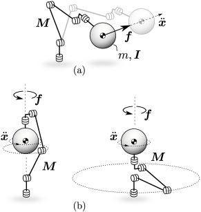
Figure 2: Dynamics-conditioned twin of an exemplary mechanism. The end effector comprises all of the mechanism’s mass $m$ and rotational inertia $\bm{I}$, which is illustrated with the oversized sphere. Links and joints are considered massless, such that their configuration has a vanishing influence on the overall dynamics.

This effect is depicted in Fig. 2b where $\bm{f}$ experiences the same rotational inertia $\bm{M}$, although having shifted most of the mechanism’s structure away from the rotatory axis in one case. In the experiments section we sample a massive number of joint configurations and show empirically that this approach indeed achieves a good homogenization of $\bm{M}^{-1}=\bm{J}\bm{H}^{-1}\bm{J}^{T}$.

IV IMPLEMENTATION

We implemented the closed loop scheme from Fig. 1 as a ROS controller in C++. The pseudo code for the IK-solving part is listed in Algorithm 1.

Algorithm 1 IK with forward dynamics

1:procedure Solver($\bm{x}^{d},\bm{q}_{0},\Delta t,N$)

2:     $\bm{\epsilon}_{0}=\bm{0}$

3:     for $i=1\text{ \bf{to} }N$ do

4:         $\bm{\epsilon}_{i}=\bm{x}^{d}-g(\bm{q}_{i-1})$

5:         $\dot{\bm{\epsilon}}_{i}=(\bm{\epsilon}_{i}-\bm{\epsilon}_{i-1})/\Delta t$

6:         $\bm{f}_{i}=\bm{K}_{p}\bm{\epsilon}_{i}+\bm{K}_{d}\dot{\bm{\epsilon}}_{i}$

7:         $\ddot{\bm{q}}_{i}=\bm{H}^{-1}(\bm{q}_{i-1})\bm{J}^{T}(\bm{q}_{i-1})\bm{f}_{i}$

8:         $\dot{\bm{q}}_{i}=0.5~{}\ddot{\bm{q}}_{i}\Delta t$ $\triangleright$ $\ddot{\bm{q}}_{i-1}\equiv\bm{0}$

9:         $\bm{q}_{i}=\bm{q}_{i-1}+0.5~{}\dot{\bm{q}}_{i}\Delta t$ $\triangleright$ $\dot{\bm{q}}_{i-1}\equiv\bm{0}$

10:     end for

11:     $\bm{q}^{d}=\bm{q}_{N}$

12:     return $\bm{q}^{d}$

13:end procedure

Note that the computation of $\bm{H}^{-1}$ and $\bm{J}^{T}$ is not part of the algorithm. For this task we used the Kinematics and Dynamics Library (KDL), which is common place in ROS. Note that the number of steps $N$ can be chosen freely to give the solver (virtual) time for any given $\bm{x}^{d}$. In combination with the gain matrices $\bm{K}_{p}$ and $\bm{K}_{d}$ this is a partially redundant means to tweak the solver to range from a one-shot IK-solver to an interpolating controller to smooth noisy targets $\bm{x}^{d}$. We discuss this behavior in the experiment on interpolation performance for low frequency sampled targets.

V EXPERIMENTS AND RESULTS

In our experiments, we chose the Universal Robot UR10 as manipulator (Fig. 3), which is ubiquitous both in industry and academia, and represents a well-known platform for many possible users. We want to emphasize, however, that our proposed IK solver has been used successfully on various manipulators. Since a central theme of this work is to use a dynamics motivated approach for IK solving instead of a pure kinematics one, we compare our method to the Jacobian transpose method where appropriate.

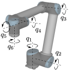
Figure 3: UR10

V-A Controller Homogenization

In this experiment we evaluated our homogenization method and compared it both to the Jacobian transpose method from (6) and a reference dynamics model. For all mechanism, we used the robot’s kinematics as provided by the ROS package.

(a)

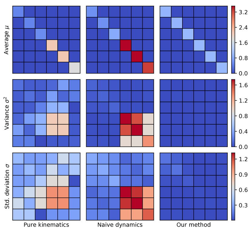
(b)

Figure 4: Experiment A. Analysis of three mapping approaches from $\bm{f}\rightarrow\ddot{\bm{x}}$ for the Universal Robots UR10. To obtain the plots, we sampled $100.000$ random configurations of $\bm{q}$ uniformly with $q_{i}\in\left[-\pi,\pi\right]$. For each sample, we computed the mapping matrix as indicated in (a). The sub figures (b) show mean, variance and standard deviation (less is better) for the individual matrix entries for the entirety of samples.

For the Jacobian transpose method , we set the gain matrix $\bm{K}$ to identity, which is a reasonable choice without further knowledge of the system.

Fig. 4(a) illustrates the qualitative distribution of mass and inertia for the experiment. We choose the following values for our proposed model (Fig. 4(a) right):

$$m =$1\text{\,}\mathrm{k}\mathrm{g}$$$ (17)

$$\bm{I} =\begin{bmatrix}1&0&0\\ 0&1&0\\ 0&0&1\end{bmatrix}~{}$\text{\,}\mathrm{k}\mathrm{g}\mathrm{m}^{2}$$$

which constitute the last link of the manipulator. For numerical stability, we set all other links to $m_{0}=10^{-3}m$ and $\bm{I}_{0}=10^{-6}\bm{I}$ respectively (instead of to zero). The reference model (Fig. 4(a) middle) had $1\text{/}6$ of $m$ and $\bm{I}$ equally attached to its links.

Fig. 4(b) shows the results of the analysis. Note that all mean matrices are in fact diagonal, as was expected for arbitrary joint space sampling. However, the variances indicate a partially strong configuration dependency for Jacobian transpose method (pure kinematic solver) and the equally conditioned mechanism (naive dynamics), indicating suboptimal solver convergence if they were applied to solve IK. Note that using dynamics does not necessarily improve homogenization (middle column). Only with the end effector approach (right column) do we effectively obtain the intended behavior.

We propose the values from (17) to be considered as good default values for a broad usage. We also take these values for the following experiments of this paper.

V-B Solver Convergence

In this experiment we analyze our control scheme from Fig. 1 for a distant IK target, using both the Jacobian transpose method and our conditioned inertia method. The distant target represents a step in Cartesian space, as illustrated in Fig. 6 for experiment B. A common use case is low-frequency sample targets. Since the speed of convergence in both systems (6) and (12) can be tweaked with the gains $\bm{K}$ and $\bm{K}_{p},\bm{K}_{d}$ respectively, we chose the following set of parameters to make the solvers comparable:

$$\Delta t=1,\bm{K}_{p} =\text{diag}(\left[1,1,1,~{}0.1,0.1,0.1\right]),$$ (18)

$$\bm{K}_{d} =\bm{0},~{}\bm{K}=\alpha\bm{I}_{6},$$

where $\alpha$ is a scaling factor built from the mean matrices from Fig. 4(b) (top row, left + right)

$$\alpha=\frac{\text{mean(diagonal}(\bm{J}\bm{H}^{-1}\bm{J}^{T}))}{\text{mean(diagonal}(\bm{J}\bm{J}^{T}))}\approx 0.7885$$ (19)

to obtain an identical mapping $\bm{f}\rightarrow\ddot{\bm{x}}$ (considering the average of the main diagonal). Fig. 5 shows the systems’ step response to a sudden Cartesian offset.

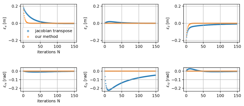
Figure 5: Experiment B. Analysis of the solver convergence for the Jacobian method: $\ddot{\bm{q}}=\alpha\bm{I}_{6}\bm{J}^{T}\bm{K}_{p}(\bm{x}^{d}-g(\bm{q}))$, and our method: $\ddot{\bm{q}}=\bm{H}^{-1}\bm{J}^{T}\bm{K}_{p}(\bm{x}^{d}-g(\bm{q}))$, with a simulation time interval of $\Delta t=$ $1\text{\,}\mathrm{s}$ and $N=150$ iterations. The plots show the six Cartesian dimensions of the error $\bm{x}^{d}-g(\bm{q})$ for each iteration.

Both systems approach the goal state, as indicated by the vanishing errors. However, there is a big difference in the intermediate solutions: The Jacobian transpose method overshoots in four out of six dimensions, and looses track of $\epsilon_{ry}$, which does not flat out for the interval observed. In comparison, our proposed method converges stronger and maintains the rotational errors constant throughout the path to the target.

V-C Interpolation Quality

In the next experiment we analyze the interpolation quality of intermediate states. For this purpose we interpolated to four targets, representing the corners of a square. The starting configuration is illustrated in Fig. 6 for experiment C. We chose $\Delta t=$0.1\text{\,}\mathrm{s}$$ and the number of iterations $N=50$ for each step. Starting at all four corners we computed $1000$ steps of intermediate states, for each taking the next counter clockwise corner as fixed target $\bm{x}^{d}$.

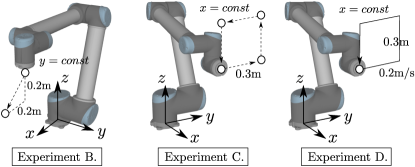
Figure 6: Robot starting configurations and target motion for three experiments.

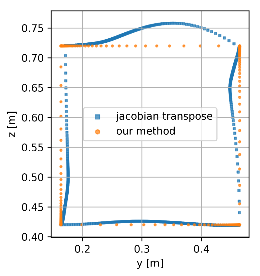
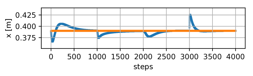
Figure 7: Experiment C. Analysis of path accuracy during interpolation to the corners of a square. We use the parameters from (18) with $\Delta t=$ $0.1\text{\,}\mathrm{s}$. The Cartesian end effector positions are computed with the robots forward kinematics $g(\bm{q})$ for each step.

Fig. 7 shows the results. The plots demonstrate that our proposed method generates goal-directed, intermediate solutions. In comparison, the Jacobian transpose method leads to distorted paths in Cartesian space. Note also that our method converges in less iterations, as indicated with bigger spaces between individual points.

V-D Motion tracking

In this experiment, we apply our method to the tracking of a moving target that follows the square from Fig. 6 for experiment D with a constant speed of $0.2\text{\,}\mathrm{m}\mathrm{/}\mathrm{s}$.

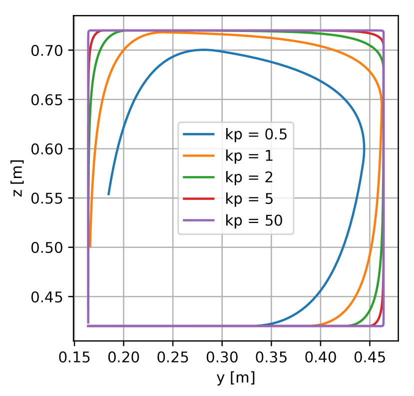
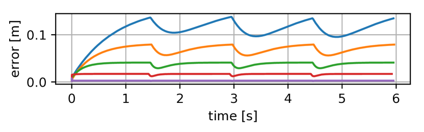
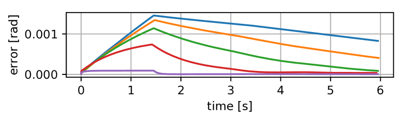
Figure 8: Experiment D. Analysis of tracking performance for a square-moving target of $0.2\text{\,}\mathrm{m}\mathrm{/}\mathrm{s}$. The family of curves is computed by varying $k_{p}$ in the gain matrix $\bm{K}_{p}=k_{p}\text{diag}(\left[1,1,1,~{}0.1,0.1,0.1\right])$. We chose $\Delta t=$0.1\text{\,}\mathrm{s}$$ and $N=10$ as IK solver parameters. Plot (a) shows the end effector’s absolute motion in Cartesian space. Plot (b) shows the according translational error $\lVert\left[\epsilon_{x}~{}\epsilon_{y}~{}\epsilon_{z}\right]^{T}\rVert$ and rotational error $\lVert\left[\epsilon_{rx}~{}\epsilon_{ry}~{}\epsilon_{rz}\right]^{T}\rVert$ to the moving target.

During the execution we sample the moving target with a frequency of $100\text{\,}\mathrm{H}\mathrm{z}$. Fig. 8 shows the tracking performance for individual gains $k_{p}$, which we use as a multiplicative factor for $\bm{K}_{p}$ from the previous experiments. The results show the intended behavior: By increasing the gains we transition from a smooth but delayed controller to a fast and exact IK solver. As an example, users may prefer $k_{p}=5$ over $k_{p}=50$ for smoothed corners for their robot control.

VI DISCUSSION

VI-A Virtual Dynamics

To obtain (9), we neglected non-linear Coriolis and gravity terms in favor of a simple, unbiased mapping from Cartesian end effector offset to joint accelerations. There are, however, scenarios in which these terms could provide beneficial features. For redundant manipulators, gravity and Coriolis terms could be used to gain more control over links and joints in the nullspace, e.g. to implement a natural behavior of moving the elbow. For manipulators with six or less degrees of freedom, however, these terms add computational complexity without real advantages.

Our algorithm does not accumulate velocity during time integration, such that the system always starts anew in each control cycle with instantaneous accelerations, having the benefit that no damping is required to avoid overshooting. Also note, that the dynamic parameters from (17), which we recommend as default values for any robotic manipulator using our IK algorithm, are not necessarily realistic, and are, in fact, deliberately off from the real system’s mass and inertia distribution. In this regard, our used term twin refers to the robot kinematics only. The dynamics are virtually conditioned to obtain an IK solver with the features as described in this work.

VI-B Controller Gains

We chose the controller gains empirically for our experiments. The configuration from Fig. 8 represents a good starting point for most use cases. The magnitude of the controller gains directly corresponds to how fine grained the solver interpolates between the sampled targets. Users can easily adapt this responsiveness according to their use case through a single factor ($k_{p}$ from Fig. 8). Additionally, the relative difference between the individual elements in the diagonal gain matrix $\bm{K}_{p}$ offers the possibility to adjust how translation is weighed against orientation, and also which Cartesian dimension gets priority in underactuated system configurations.

VI-C Efficiency

Computing the inverse of the manipulator’s mass matrix in each controller cycle introduces additional computational cost. However, we did not experience this to become a performance issue, even for solver iteration rates of $10\text{\,}\mathrm{k}\mathrm{H}\mathrm{z}$, which we tested on an Intel^® Core™ i7-4900MQ. Experiment C showed that our solver converges in substantially less iterations. Weighing this advantage against the more complex computation scheme in terms of overall convergence time could be subject to further study.

VII CONCLUSIONS

In this work we presented a new method for sample-based motion tracking for robotic manipulators. The core concept of our approach bases on including the mass matrix of a virtually conditioned twin of the manipulator into the control loop for solving IK. Deriving our concept from the view of manipulator forward dynamics simulations, we offer an intuitive solution to achieve task space homogenization despite varying robot joint configurations, for which we provided an empirical proof on the UR10 robot. We tested and compared our method in experiments with the UR10 to the well-known Jacobian transpose method. The results showed that our solution outperforms the Jacobian transpose method in terms of convergence, path accuracy and interpolation quality. Users may configure the algorithm to anything from a smooth controller to a fast and accurate IK solver, also for applications outside the context of robot motion tracking.

References

- [1] Andreas Aristidou, Joan Lasenby, Yiorgos Chrysanthou and Ariel Shamir “Inverse Kinematics Techniques in Computer Graphics: A Survey” In Computer Graphics Forum 37.6, 2018, pp. 35–58 Wiley Online Library URL: https://onlinelibrary.wiley.com/doi/full/10.1111/cgf.13310
- [2] Rosen Diankov et al. “Manipulation planning for the jsk kitchen assistant robot using openrave” In The 29th Annual Conference on Robotics Society of Japan, AC2Q2–2, 2011
- [3] William A Wolovich and H Elliott “A computational technique for inverse kinematics” In The 23rd IEEE Conference on Decision and Control, 1984, pp. 1359–1363 URL: http://ieeexplore.ieee.org/abstract/document/4048118/
- [4] A Balestrino, G De Maria and L Sciavicco “Robust control of robotic manipulators” In IFAC Proceedings Volumes 17.2 Elsevier, 1984, pp. 2435–2440 URL: http://www.sciencedirect.com/science/article/pii/S1474667017613478
- [5] Alexandre N Pechev “Inverse kinematics without matrix inversion” In IEEE International Conference on Robotics and Automation (ICRA), 2008, pp. 2005–2012 URL: http://ieeexplore.ieee.org/abstract/document/4543501/?reload=true
- [6] Yoshihiko Nakamura and Hideo Hanafusa “Inverse kinematic solutions with singularity robustness for robot manipulator control” In ASME, Transactions, Journal of Dynamic Systems, Measurement, and Control 108, 1986, pp. 163–171
- [7] CW Wampler and LJ Leifer “Applications of damped least-squares methods to resolved-rate and resolved-acceleration control of manipulators” In Journal of Dynamic Systems, Measurement, and Control 110.1 American Society of Mechanical Engineers, 1988, pp. 31–38
- [8] Patrick Beeson and Barrett Ames “TRAC-IK: An Open-Source Library for Improved Solving of Generic Inverse Kinematics” In IEEE-RAS International Conference on Humanoid Robots (Humanoids), 2015 URL: https://ieeexplore.ieee.org/abstract/document/7363472
- [9] Samuel R Buss and Jin-Su Kim “Selectively damped least squares for inverse kinematics” In Journal of Graphics tools 10.3 Taylor & Francis, 2005, pp. 37–49 URL: https://www.tandfonline.com/doi/abs/10.1080/2151237X.2005.10129202
- [10] Morgan Quigley et al. “ROS: an open-source Robot Operating System” In ICRA workshop on open source software 3.3.2, 2009, pp. 5 URL: http://www.willowgarage.com/papers/ros-open-source-robot-operating-system
- [11] Sachin Chitta et al. “ros_control: A generic and simple control framework for ROS” In The Journal of Open Source Software, 2017 DOI: 10.21105/joss.00456
- [12] John J Craig “Introduction to robotics: mechanics and control, 3/E” Pearson Education India, 2009
- [13] S. Scherzinger, A. Roennau and R. Dillmann “Forward Dynamics Compliance Control (FDCC): A new approach to cartesian compliance for robotic manipulators” In IEEE/RSJ International Conference on Intelligent Robots and Systems (IROS), 2017, pp. 4568–4575 DOI: 10.1109/IROS.2017.8206325