From deterministic dynamics to thermodynamic laws II: Fourier’s law and mesoscopic limit equation

Abstract.

This paper considers the mesoscopic limit of a stochastic energy exchange model that is numerically derived from deterministic dynamics. The law of large numbers and the central limit theorems are proved. We show that the limit of the stochastic energy exchange model is a discrete heat equation that satisfies Fourier’s law. In addition, when the system size (number of particles) is large, the stochastic energy exchange is approximated by a stochastic differential equation, called the mesoscopic limit equation.

1. Introduction

Fourier’s law is an empirical law describing the relationship between the thermal conductivity and the temperature profile. In 1822, Fourier concluded that “the heat flux resulting from thermal conduction is proportional to the magnitude of the temperature gradient and opposite to it in sign” [14]. The well-known heat equation is derived based on Fourier’s law. However, the rigorous derivation of Fourier’s law from microscopic Hamiltonian mechanics remains to be a challenge to mathematicians and physicist [3]. This challenge mainly comes from our limited mathematical understanding to nonequilibrium statistical mechanics. After the foundations of statistical mechanics were established by Boltzmann, Gibbs, and Maxwell more than a century ago, many things about nonequilibrium steady state (NESS) remains unclear, especially the dependency of key quantities on the system size $N$.

There have been several studies that aim to derive Fourier’s law from the first principle. A large class of models [29, 31, 12, 11, 10] use anharmonic chains to describe heat conduction in insulating crystals. The ergodicity (existence, uniqueness, and the speed of convergence) of nonequilibrium steady states for some (but not all) of anharmonic chains can be rigorously proved [29, 30]. Entropy production rate can also be studied in some cases [31, 33, 32, 4, 11]. Also, the limiting dynamics of energy profiles of some weakly interacting Hamiltonian system follows Ginzburg-Landau dynamics, whose scaling limit is a nonlinear heat equation [9, 28]. But in general, Fourier’s law can only be proved for some simple Hamiltonian models and energy exchange models [2, 22]. Other studies consider dynamical billiards systems, which largely resembles the heat conduction in ideal gas. Rigorous results beyond ergodicity is extremely difficult when a system involves multiple interacting particles [36, 35, 5]. But many non-rigorous results are available. For example, many recent studies [26, 19, 34] consider the Markov energy exchange models obtained from non-rigorous derivations in [17, 16, 18]. Also see [23] for a review of many numerical and analytical results.

The aim of this series of paper is to derive macroscopic thermodynamic laws, including Fourier’s law, from deterministic billiards-like models. As stated above, a fully rigorous derivation is extremely difficult due to the limited mathematical understanding to billiards systems with multiple interacting particles. Hence the philosophy of this series is to use as much rigorous study as possible, and connecting gaps between pieces of rigorous works by numerical results. The subject of this study is a dynamical system that models heat conduction in gas. Consider a long and thin 2D billiard table that is connected with two heat baths with different temperatures. Many disk-shaped moving particles are placed in the tube. Particles move and interact freely through elastic collisions. When a particle hits the heat bath, it receive a random force whose statistics depends on the boundary temperature. Needless to say, this is not a mathematically tractable problem. We lose control of a particle once it moves into the tube.

In [25], we impose a localization to this billiard-like model by adding a series of barriers into the tube. This divides a tube to a chain of cells. Particles can collide through opennings on the barrier but can not pass the barrier. The motivation is that the mean free path of realistic gas particles is as short as 68 nm at ambient pressure [20]. Similar idea of localization is also reported in [6]. Then we use numerical simulation to study the statistics of energy exchanges between cells. Because of the localization, energy exchange can only be made through “effective collisions”, which means collisions between two particles from adjacent cells through the opening on the barrier. The time distribution of effective collisions and the rule of energy exchange during an effective collision are studied. A stochastic energy exchange model is then obtained in [25]. Additional numerical simulation shows that this stochastic energy exchange model preserves the key asymptotical dynamics of the original billiards-like model.

In this paper, we continue to work on the mesoscopic limit of the stochastic energy exchange model derived in [25] and further studied in [24]. Still consider the ideal gas at ambient pressure. If the size of a cell is at the same scale of the mean free path, then a cell should contain $10^{4}\sim 10^{5}$ particles. Therefore, we should work on the stochastic energy exchange model with a large number of particles in each cell. In this senario, each energy exchange only changes a small proportion of the total cell energy. To maintain the thermal conductivity unchanged, some geometric rescaling and time rescaling is necessary. When the number of particles per cell increases, the size and mass of each particle must decrease correspondingly. Then we need to rescale the time if necessary, such that particles can not pass these openings, but the order of magnitude of the mean heat flux can be preserved. Let $M$ be the number of particles per cell. The goal of the rescaling is to make the number of energy exchange per unit time $O(M)$, and the mean heat flux $O(1)$.

We work on the stochastic energy exchange model after the geometric and time rescaling. The rule of energy redistributions still follow from what we have obtained in [25]. The resultant stochastic energy exchange model resemble a slow-fast dynamical system when there are many particles in each cell. Small energy exchanges occur with high frequency. Each energy exchange can be described by a function of the current energy configuration and a few i.i.d. random variables. This motivates us to study the law of large numbers and the central limit theorem when $M$ approaches to infinity. We call it the mesoscopic limit, because the observable under consideration is now the total energy of $10^{4}\sim 10^{5}$ particles. Our calculation reveals that the mesoscopic dynamics of the stochastic energy exchange model mimics the Landau-Ginzburg dynamics, which appears in the scaling limit of a number of Hamiltonian systems.

The technique used in this paper, namely the martingale problem, is classical. It was proposed in 1970s and successfully used to study the scaling limit of chemical reaction systems and slow-fast hyperbolic dynamical systems [7, 1, 38]. We first use the result in [13] to show the tightness of a sequence of random processes. Then the limit is given by the uniqueness of the solution to the martingale problem. In some estimations, it is particularly important to “prescribe the randomness” to the energy exchange model. This allows us to “decouple” dependent variables after some relaxation. After decoupling, we can work on independent random variables. We remark that these techniques has been applied in our earlier papers [27, 24]. We set up two martingale problems to prove the law of large numbers and the central limit theorem respectively.

The law of large number shows that at the infinite-particle limit, the stochastic energy exchange model converges to a nonlinear discrete heat equation. In addition, this equation admits a stable equilibrium. The energy flux starting from this stable equilibrium can be explicitly given. Hence Fourier’s law is easily derived from the equilibrium of this discrete heat equation. At ambient pressure, $M$ is only $10^{4}$ to $10^{5}$. Therefore, random fluctuations, which is in the magnitude of $O(M^{-1/2})$, should not be neglected. This motivates us to further study the central limit theorem.

The central limit theorem shows that the rescaled difference between the stochastic energy exchange model and the nonlinear discrete heat equation is given by a timely dependent stochastic differential equation. Combine estimates from the law of large numbers and the central limit theorem. Some easy calculations show that the stochastic energy exchange model is then approximated by a stochastic differential equation with $O(M^{-1/2})$ random perturbation term. We call this stochastic differential equation the mesoscopic limit equation. As will be discussed in the conclusion, the nonequilibrium steady state of this mesoscopic limit equation can be explicitly approximated by a WKB expansions. As a result, many properties, including the long range correlations like the one given in [37], entropy production rates, and fluctuation-dissipation theorems can be proved by working on this mesoscopic limit equation. Fourier’s law of the NESS of the stochastic energy exchange model, which is a stronger result than the Fourier’s law proved in this paper, can also be proved. We decide to put these results into our subsequent work.

The organization of this paper is as follows. In Section 2, we review the main result of [25], introduce the model setting, and describe the stochastic energy model under the geometric rescaling. Section 3 gives the main result. The main strategy of proof is described in Section 4. The law of large numbers and Fourier’s law are proved in Section 5. Section 6 is about the central limit theorem and the mesoscopic limit equation. Section 7 is the conclusion.

2. From billiard dynamics to stochastic energy exchange model

2.1. Billiards model with time rescaling

Consider an 1D chain of $N$ billiard tables (see Figure 1) in $\mathbb{R}^{2}$ that are connected through nearest neighbors, denoted by $\Omega_{1},\cdots,\Omega_{N}$. We assume each table is a subset of $\mathbb{R}^{2}$ whose boundary is formed by finitely many piecewise $C^{3}$ curves that are either flat or convex inward. This assumption makes the billiard system chaotic. Then we place $M$ disk-shaped particles into each cell. The radius of each particle is $RM^{-1/2}$, and the mass of each particle is $2M^{-1}$. Hence the total area of particles equals $\pi R^{2}$ and the total mass of particles equals $2$. In addition, a barrier with a hole is placed between each adjacent pair of cells. The size of the hole is $2(1-\epsilon)RM^{-1/2}$ with $\epsilon\ll 1$, so that particles can not pass the hole.

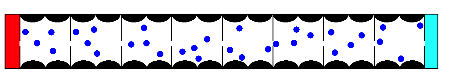
Figure 1. An 1D chain of billiard tables connected with two heat baths. $M=4$ particles are “trapped” in each cell. A barrier with a hole is placed between adjacent cells, such that particles can collide through the hole, but cannot pass it.

Particles can move freely until colliding with the cell boundary (including the barrier) or other particles. We assume the following for this billiard system.

• A particle is trapped by barriers and will never leave its cell.

• Particles from neighbor cells can collide through holes on the barrier.

• All collisions are elastic. Particles do not rotate.

• The billiard system in each cell is chaotic.

• $R$ is small enough such that particles would not get stuck.

• $R$ is small enough such that particles can be completely out of reach by their neighbors.

It remains to prescribe the boundary condition. We assume that this chain is coupled with two heat baths through the left and right cells. The heat bath is a billiard table with the same geometric configuration but randomly chosen total kinetic energy. After a collision between a heat bath particle and a “regular” particle, a random total energy $E_{L}$ (resp. $E_{R}$) is chosen for the left (resp. right) heat bath from the exponential distribution with mean $T_{L}$ (resp. $T_{R}$). Then all heat bath particles are redistributed such that their positions and velocities satisfy the conditional Liouville measure (conditioning on the conservation of total energy). The system evolves deterministically between redistributions of heat bath particles.

The first paper in this series [25] numerically shows the following results.

• The time between two consecutive collisions through the barrier is exponentially distributed with a rate that can be approximated by $\min\{E_{1},E_{2}\}$ if $\min\{E_{1},E_{2}\}\ll 1$, where $E_{1}$ and $E_{2}$ represent the total energy in two cells respectively.

• The energy carried by the particle that participates a collision through the barrier can be approximated by a Beta distribution with parameters $(1,M-1)$.

• The energy redistribution during a collision can be approximated by a uniform random redistribution.

None of these approximation is precise. But further studies in [25] confirms that these approximations preserve both the asymptotic dynamics and the scaling of the thermal conductivity.

One thing not studied in [25] is the asymptotic dependence of collision rate on $M$. Heuristically, when $M$ is large, the mean energy carried by each particle is only $O(M^{-1})$. In order to model the heat conduction, we need to rescale the time to make $O(M)$ collisions per unit time. In this paper, we consider the problem at two different time scales. Let $\phi(M)$ be the number of collisions per unit time depending on $M$. The time rescaling $t\rightarrow t/\phi(M)$ gives the slow scale problem, at which only $O(1)$ collision through the barrier occurs per unit time. The time rescaling $t\rightarrow M\phi(M)^{-1}t$ gives the fast scale problem, at which the collision rate is $O(M)$. Our fundamental goal is to study the limit laws of the fast scale problem. But the slow-scale problem makes many calculations and explanations easier. Then the time distribution between two consecutive collisions be an exponential distribution with rate $f(E_{1},E_{2})$ (resp. $Mf(E_{1},E_{2})$) for the slow (resp. fast) scale problem, where $f$ is a rate function, and $E_{1},E_{2}$ are the total energy stored in corresponding cells. Note that in this paper we consider a generic rate function $f(E_{1},E_{2})$ that satisfies a few mild assumptions. If one take the rare collision limit first, then rescale the time back, as did in [17, 16], the resultant rate function may be different.

The explicit formula of $\phi(M)$ is not straightforward. We demonstrate a billiard system with two cells as an example. The total area of particles in each cell equals to $\pi$. The geometric configuration is shown in Figure 2 top. Then we record the number of collisions at the barrier and the energy of particles that collide at the barrier for $M=1,2\cdots,50$. In Figure 2 bottom left, we compute the frequency of collisions through the barrier, which is the time rescaling function $\phi(M)$ needed for the slow-scale system. The bottom right panel of Figure 2 shows $M$ times the mean energy of particles that collide through the barrier. Although some bias occurs when there are only a few particles, we can see that the scaling of mean energy of a particle that participates a collision is stabilized at $O(M^{-1})$.

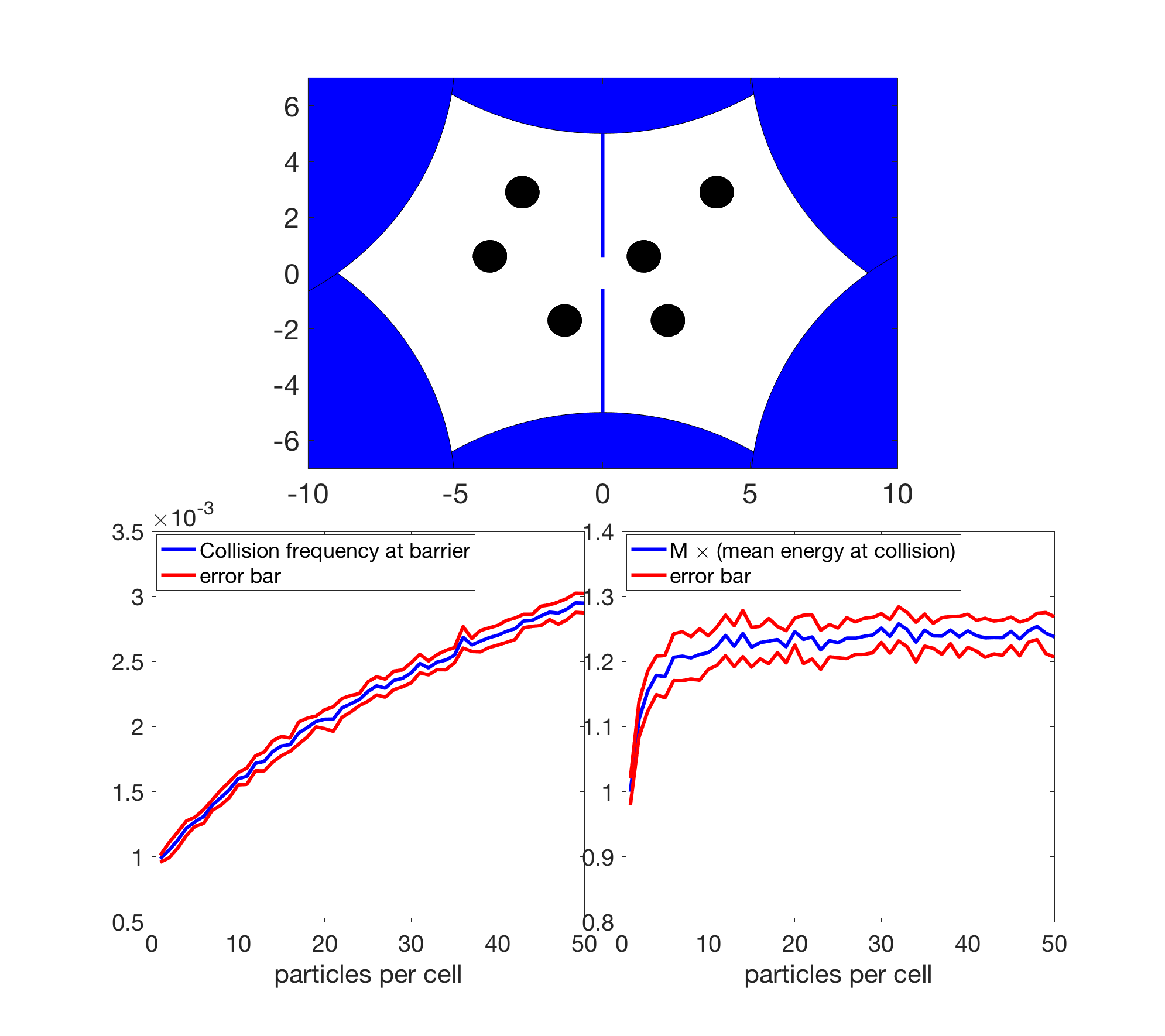
Figure 2. Top: An example of two cells with a barrier and no heat bath. Each cell has $3$ particles inside of it. Bottom left: Frequency of collision through the barrier. Red plot represents the error bar with one standard deviation. Bottom right: $M$ times the mean energy of particles that participate collisions through the barrier. Red plot represents the error bar with one standard deviation.

2.2. Stochastic energy exchange model

After rescaling the time by $\phi(M)$, we obtain the following slow-scale stochastic energy exchange model. Consider a chain of $N$ cells $1,2,\cdots,N$ connected to two heat baths with temperatures $T_{L}$ and $T_{R}$ respectively. Each cell contains a certain amount of energy, denoted by $E_{1},\cdots,E_{N}$. Let $M$ be a model parameter that corresponds to the number of moving particles of the original kinetic model. The rule of energy exchange is as follows.

Assume there exists a rate function $f(E_{1},E_{2})$ that satisfies the following three assumptions:

• $f$ is $C^{1}$ continuous and strictly positive for $E_{1},E_{2}>0$.

• $f$ is non-decreasing with respect to both $E_{1}$ and $E_{2}$.

• There exists a constant $K<\infty$ such that $f(E_{1},E_{2})<K$ uniformly.

The first two assumptions are heuristic. The energy exchange rate must be positive and continuous. Higher cell energy must have higher energy exchange rate. The third assumption is technical. In [25] we have showed that the stochastic energy exchange model admits an invariant probability measure. Hence the probability of having very high cell energy is low. Assuming all clock rates being below a large constant will not significantly change the dynamics. On the other hand, “overheating” Poisson clocks will cause many technical troubles. The aim of this paper is to prove the limit law. Without assumption (c), this paper will be significantly distracted the effort of controlling “overheating” Poisson clocks.

An exponential clock with rate $f(E_{i},E_{i+1})$ is associated to a pair of cells $i$ and $i+1$. All exponential clocks are mutually independent. When the clock rings, cells $i$ and $i+1$ exchange their energy such that

$$E_{i}^{\prime}=E_{i}-B_{1}E_{i}+p(B_{1}E_{i}+B_{2}E_{i+1})$$

$$E_{i+1}^{\prime}=E_{i+1}-B_{2}E_{i+1}+(1-p)(B_{1}E_{i}+B_{2}E_{i+1})\,,$$

where $E_{i}^{\prime}$ and $E_{i+1}^{\prime}$ denote post-exchange energy, $p$ is a uniform random variable on $(0,1)$, and random variables $B_{1},B_{2}$ are two independent Beta random variables with parameters $1,M-1$. In other words, each cell contribute a small proportion of its energy for the redistribution. The rule of energy exchange with boundary is similar. Two additional exponential clocks are associated to two ends of the chain with rates $f(T_{L},E_{1})$ and $f(E_{N},T_{R})$. When the clock rings, rules of update are

$$E_{1}^{\prime}=E_{1}-B_{1}E_{1}+p(B_{1}E_{1}+B_{2}Exp(T_{L}))$$

and

$$E_{N}^{\prime}=E_{N}-B_{1}E_{N}+p(B_{1}E_{N}+B_{2}Exp(T_{R}))\,,$$

where $Exp(\lambda)$ means an exponential random variable with mean $\lambda$, $B_{1},B_{2}$, and $p$ are same as before. For the sake of consistency, sometimes we use notations $E_{0}=T_{L}$ and $E_{N+1}=T_{R}$. In addition, we denote the exponential clock between $E_{i}$ and $E_{i+1}$ by “clock $i$”.

It is easy to see that this stochastic energy exchange model gives a Markov chain $\Phi^{M}_{t}$ on $\mathbb{R}^{N}$, where $M$ is a model parameter. For the sake of being consistent, we still denote the $i$-th entry of $\Phi^{M}_{t}$ by $E_{i}(t)$ if it leads to no confusion.

2.3. An alternative description

We provide the following alternative description of $\Phi^{M}_{t}$ that fits the calculation in this paper better. Obviously $\Phi^{M}_{t}$ is a Markov jump process in $\mathbb{R}^{N}$. Assume $0=t_{0}<t_{1}<\cdots$ are jump time of $\Phi^{M}_{t}$. Then $t_{i+1}-t_{i}$ has exponential distribution with rate

$$R(\Phi^{M}_{t_{i}})=\sum_{i=1}^{N-1}f(E_{i}(t_{i}),E_{i+1}(t_{i}))+f(T_{L},E_{1}(t_{i}))+f(E_{N}(t_{i}),T_{R})=\sum_{i=0}^{N}f(E_{i}(t_{i}),E_{i+1}(t_{i}))\,.$$

We “prescribe” the randomness such that

$$t_{i+1}-t_{i}=-R(\Phi^{M}_{t_{i}})^{-1}\log(1-q_{i})\,,$$

where $\{q_{i}\}$ is an i.i.d. sequence of uniform random variables on $(0,1)$.

In addition, we have

$$\Phi^{M}_{t_{i}+}=\Phi^{M}_{t_{i}}+X^{M}_{i}\,,$$

where $X^{M}_{i}$ is a random variable that depends on $\Phi^{M}_{t_{i}}$ in a way that

$$X^{M}_{i}=\zeta(\Phi^{M}_{t_{i}},\omega^{M}_{i})\,,$$

where $\omega^{M}_{i}=(p^{(i)}_{1},p^{(i)}_{2},p^{(i)}_{3},B^{(i)}_{1},B^{(i)}_{2})$ is a sequence of i.i.d. random vectors. $\omega^{M}_{i}$ has five entries, among which $p^{(i)}_{1},p^{(i)}_{2},p^{(i)}_{3}$ are three i.i.d. uniform random variables on $(0,1)$, and $B^{(i)}_{1},B^{(i)}_{2}$ are two i.i.d. Beta random variables with parameters $(1,M-1)$.

The definition of the function $\zeta$ is as follows. $p^{(i)}_{1}$ is used to select exponential clocks. For $0\leq k\leq N$, clock $k$ is chosen if

$$\frac{1}{R(\Phi^{M}_{t_{i}})}\sum_{j=0}^{k}f(E_{j}(t_{i}),E_{j+1}(t_{i}))\leq p^{(i)}_{1}<\frac{1}{R(\Phi^{M}_{t_{i}})}\sum_{j=0}^{k+1}f(E_{j}(t_{i}),E_{j+1}(t_{i}))\,.$$

$p^{(i)}_{2}$ is used to choose the heat bath energy if and only if clock $0$ or clock $N$ is chosen. $p^{(i)}_{3}$ determines the energy redistribution. And $B_{1}^{(i)}$ and $B_{2}^{(i)}$ are two Beta random variables involved in the energy exchange event. More precisely, we have

(2.1) $$\zeta(\Phi^{M}_{t_{i}},\omega^{M}_{i})=\left\{\begin{array}[tb]{lll}-J_{k}\mathbf{e}_{k}+J_{k}\mathbf{e}_{k+1}&\mbox{ if }&\mbox{ clock }k\mbox{ is chosen}\,,1\leq k\leq N-1\\ J_{0}\mathbf{e}_{1}&\mbox{ if }&\mbox{ clock }0\mbox{ is chosen,}\\ -J_{N}\mathbf{e}_{N}&\mbox{ if }&\mbox{ clock }N\mbox{ is chosen,}\end{array}\right.$$

where $\mathbf{e}_{k}$ is the $k$-th vector of the standard basis, and

$$J_{k}=\left\{\begin{array}[tb]{lll}(1-p_{3}^{(i)})B^{(i)}_{1}E_{k}(t_{i})-p^{(i)}_{3}B_{2}^{(i)}E_{k+1}(t_{i})&\mbox{ if }&1\leq k\leq N-1\\ -(1-p_{3}^{(i)})B^{(i)}_{1}T_{L}\log(1-p^{(i)}_{2})-p^{(i)}_{3}B_{2}^{(i)}E_{1}(t_{i})&\mbox{ if }&k=1\\ (1-p_{3}^{(i)})B^{(i)}_{1}E_{N}(t_{i})+p^{(i)}_{3}B_{2}^{(i)}T_{R}\log(1-p^{(i)}_{2})&\mbox{ if }&k=N\end{array}\right.$$

is the net flux from cell $k$ to cell $k+1$.

This alternative description is less straightforward. But it “prescribes” all randomness in this stochastic energy process. We will need this soon in our calculations.

3. Main Result

$\Phi^{M}(t)$ is a Markov jump process at the slow scale, at which the energy flux is $O(M^{-1})$ for increasing $M$. The main result of this paper is about the limit law of the fast scale problem with $O(1)$ energy flux. To make the limit law work, we consider the following process $\Theta^{M}(t)$ at the fast scale with

$$\Theta^{M}(t_{i}/M)=\Phi^{M}(t_{i})\quad\mbox{ for }t_{i}\leq t<t_{i+1}$$

where $0=t_{0}<t_{1}<\cdots<t_{n}<\cdots$ are energy exchange times for $\Phi^{M}(t)$. Sample paths of $\Theta^{M}(t)$ are right continuous with left limits. This makes $\Theta^{M}(t)\in D([0,T])$, the Skorokhod space on $[0,T]$.

The first result is about the law of large number of $D[0,T]$.

Theorem 1 For any finite $T>0$,

$$\lim_{M\rightarrow\infty}\Theta^{M}(t)=\bar{\Theta}(t)$$

almost surely for any $t\in[0,T]$, where $\bar{\Theta}(t)$ solves the ordinary differential equation

(3.1) $$\frac{\mathrm{d}}{\mathrm{d}t}\bar{\Theta}(t)=F(\bar{\Theta}(t))\,,$$

where

$$F_{i}(\bar{\Theta}(t))=\frac{1}{2}f(\bar{\Theta}_{i-1}(t),\bar{\Theta}_{i}(t))(\bar{\Theta}_{i-1}(t)-\bar{\Theta}_{i}(t))+\frac{1}{2}f(\bar{\Theta}_{i}(t),\bar{\Theta}_{i+1}(t))(\bar{\Theta}_{i+1}(t)-\bar{\Theta}_{i}(t))$$

for $i=1,\cdots,N$. Here we use the boundary condition $\bar{\Theta}_{0}=T_{L}$ and $\bar{\Theta}_{N+1}=T_{R}$.

The Fourier’s law with respect to $\bar{\Theta}(t)$ is straightforward. We have the following proposition.

Proposition 2 The flow determined by equation (3.1) admits a stable equilibrium $E^{*}$. Let $\kappa$ be the expected energy flux starting from $E^{*}$ (defined in equation (LABEL:kappa)), we have $\kappa=\frac{1}{2}f(T_{L},T_{L})+O(T_{R}-T_{L})$ if $|T_{R}-T_{L}|\ll 1$.

Let

$$\Gamma^{M}(t)=\sqrt{M}(\Theta^{M}(t)-\bar{\Theta}(t))\,.$$

The following theorem gives the central limit theorem for $\Theta^{M}(t)$.

Theorem 3 For any finite $T>0$,

$$\lim_{M\rightarrow\infty}\Gamma^{M}(t)=\bar{\Gamma}(t)$$

almost surely for any $t\in[0,T]$, where $\bar{\Gamma}(t)$ solves the time-dependent stochastic differential equation

(3.2) $$\mathrm{d}\bar{\Gamma}(t) = DF(\bar{\Theta}(t))\bar{\Gamma}(t)\mathrm{d}t+H(\bar{\Theta}(t))\mathrm{d}\mathbf{W}_{t}$$

$$\bar{\Gamma}(0) = 0\,,$$

where $DF$ is the Jacobian matrix of $F$ given in equation (3.1),

$$H(\mathbf{E})=\begin{bmatrix}V_{0}(T_{L},E_{1})&V(E_{1},E_{2})&0&0&\cdots&\cdots\\ 0&V(E_{1},E_{2})&V(E_{2},E_{3})&0&\cdots&\cdots\\ \vdots&\vdots&\vdots&\vdots&\vdots&\vdots\\ 0&\cdots&\cdots&0&V(E_{N-1},E_{N})&V_{N}(E_{N},T_{R})\\ \end{bmatrix}$$

is an $N\times(N+1)$-matrix valued function on $\mathbb{R}^{N}$,

$$V(x_{1},x_{2})=\sqrt{f(x_{1},x_{2})\left(\frac{2}{3}x_{1}^{2}-\frac{1}{3}x_{1}x_{2}+\frac{2}{3}x_{2}^{2}\right)}\,,$$

$$V_{0}(x_{1},x_{2})=\sqrt{f(x_{1},x_{2})\left(\frac{4}{3}x_{1}^{2}-\frac{1}{3}x_{1}x_{2}+\frac{2}{3}x_{2}^{2}\right)}\,,$$

and

$$V_{N}(x_{1},x_{2})=\sqrt{f(x_{1},x_{2})\left(\frac{2}{3}x_{1}^{2}-\frac{1}{3}x_{1}x_{2}+\frac{4}{3}x_{2}^{2}\right)}\,,$$

and $\mathrm{d}\mathbf{W}_{t}$ is the white noise in $\mathbb{R}^{N+1}$.

Theorem 1 and Theorem 2 imply that $\Theta^{M}(t)$ is approximated by a stochastic differential equation.

Proposition 4 Let $Z_{t}$ be a stochastic differential equation satisfying

(3.3) $$\mathrm{d}Z_{t}=F(Z_{t})\mathrm{d}t+M^{-1/2}H(Z_{t})\mathrm{d}W_{t}\,.$$

Then we have

(3.4) $$\mathbb{E}[\|\Theta^{M}(t)-Z_{t}\|]<CM^{-1},$$

where $C<\infty$ is a constant that is independent of $t\in[0,T]$ and $M$.

Equation (3.3) is called the mesoscopic limit equation.

Proof of main theorems.

Theorem 1 follows from Theorem 5.1. Lemma 5.9, 5.10, and 5.11 together imply Proposition 2. Theorem 3 is proved in Section 6 in Theorem 6.1. Proposition 4 is Corollary 6.8 in Section 6. ∎

4. Strategy of proof

The proof of limiting laws regarding $\Theta^{M}(t)$ and $\Gamma^{M}(t)$ can be divided into the following three steps.

1. Tightness. The first step is to show that the collection of probability measures on $D([0,T],\mathbb{R}^{N})$ generated by $\Theta^{M}(t)$ (and $\Gamma^{M}(t)$) is tight. This means $\Theta^{M}(t)$ (and $\Gamma^{M}(t)$) has accumulation points as $M\rightarrow\infty$. Throughout this paper, we assume that $D([0,T],\mathbb{R}^{N})$ is equipped with the canonical Skorokhod metric and the Borel sigma field from it. The tightness in Skorokhod space follows from the following well known result.

Theorem 4.1 (Theorem 3.8.6 of [13]).

A sequence of $\mathbb{R}^{n}$-valued stochastic process $X_{n}(t),t\in[0,\infty]$ is tight in $D([0,\infty],\mathbb{R}^{n})$ if and only if

• For any $T>0$, there exist $\beta>0$ and random variable $\gamma_{n}(\delta,T)$ such that for $0\leq t\leq T$, $0\leq u\leq\delta$, and $0\leq v\leq\min\{t,\delta\}$,

  $$\mathbb{E}[\min\left\{q^{\beta}(X_{n}(t+u),X_{n}(t)),q^{\beta}(X_{n}(t),X_{n}(t-v))\right\}\,|\,\mathcal{F}^{n}_{t}] \leq\mathbb{E}[\gamma_{n}(\delta,T)\,|\,\mathcal{F}^{n}_{t}]$$

  $$\lim_{\delta\rightarrow 0}\limsup_{n\rightarrow\infty}\mathbb{E}[\gamma_{n}(\delta,T)] =0$$

• $$\lim_{\delta\rightarrow 0}\limsup_{n\rightarrow\infty}\mathbb{E}[q^{\beta}(X_{n}(\delta),X_{n}(0))]=0\,,$$

  where $q(x,y)=\min\{1,|x-y|\}$.

2. Martingale problem. The next step is to show that any accumulation point of $\Theta^{M}(t)$ (and $\Gamma^{M}(t)$) satisfies a martingale problem. We have the following definition.

Definition 4.2.

Let $\mathcal{L}$ be a linear operator such that the domain of $\mathcal{L}$ is a subset of the Banach space of all bounded Borel measurable functions on $\mathbb{R}^{N}$. A triple $((\Omega,\mathcal{F},\mathbf{P}),(\mathcal{F}_{t})_{t\geq 0},(X_{t})_{t\geq 0})$ with $((\Omega,\mathcal{F},\mathbf{P}),(\mathcal{F}_{t})_{t\geq 0})$ a stochastic basis and $X_{t}$ a $\mathcal{F}_{t}$ adapted stochastic process on $\mathbb{R}^{N}$ is a solution of the martingale problem for $\mathcal{L}$ if for all $f$ in the domain of $\mathcal{L}$,

$$f(X_{t})-f(X_{0})-\int_{0}^{t}(\mathcal{L}f)(X_{s})\mathrm{d}s,\quad t\geq 0$$

is a martingale with respect to $\mathcal{F}_{t}$.

A martingale problem is said to be well posed if there exists a unique solution $X_{t}$. Martingale problem is a very powerful tool. An obvious solution to the martingale problem is the stochastic process whose infinitesimal generator is $\mathcal{L}$.

3. Uniqueness of solution to the martingale problem. It remains to show that the maringale problem with respect to $\Theta^{M}(t)$ (and $\Gamma^{M}(t)$) has a unique solution. In general, let $\mathcal{L}$ be the generator of a stochastic differential equation, then the martingale problem with respect to $\mathcal{L}$ has a unique solution if and only if the corresponding stochastic differential equation has a unique weak solution. We refer [38] for further reference regarding the uniqueness of solutions to martingale problems. The following theorem will be used in our proof.

Theorem 4.3 (Theorem 10.2.2 of [38]).

If for each $T>0$, there exists a constant $C_{T}<\infty$ such that

$$\sup_{0\leq t\leq T}\|a(t,x)\|\leq C_{T}(1+|x|^{2}),\quad\mbox{for }x\in\mathbb{R}^{d}$$

and

$$\sup_{0\leq t\leq T}x\cdot b(t,x)\leq C_{T}(1+|x|^{2}),\quad\mbox{for }x\in\mathbb{R}^{d}\,,$$

then the martingale problem for generator

$$L_{t}=\frac{1}{2}\sum_{i,j}^{N}a_{i,j}(t,\cdot)\frac{\partial^{2}}{\partial x_{i}\partial x_{j}}+\sum_{i=1}^{N}b_{i}(t,\cdot)\frac{\partial}{\partial x_{i}}$$

is well posed.

5. Averaging principle and Fourier’s law

5.1. Law of Large Numbers

We denote the rescaled expectation of $X^{M}_{i}$ by

$$\mathbb{E}[X^{M}_{i}]=\frac{1}{M}\bar{\zeta}(\Phi^{M}_{t_{i}})\,.$$

It is easy to see that

$$\bar{\zeta}=\frac{1}{R(\Phi^{M}_{t_{i}})}\begin{bmatrix}\frac{1}{2}f(T_{L},E_{1}(t_{i}))(T_{L}-E_{1}(t_{i}))+\frac{1}{2}f(E_{1}(t_{i}),E_{2}(t_{i}))(E_{2}(t_{i})-E_{1}(t_{i}))\\ \vdots\\ \frac{1}{2}f(E_{k}(t_{i}),E_{k+1}(t_{i}))(E_{k+1}(t_{i})-E_{k}(t_{i}))+\frac{1}{2}f(E_{k-1}(t_{i}),E_{k}(t_{i}))(E_{k-1}(t_{i})-E_{k}(t_{i}))\\ \vdots\\ \frac{1}{2}f(E_{N}(t_{i}),E_{1}(t_{i}))(T_{R}-E_{N}(t_{i}))+\frac{1}{2}f(E_{N-1}(t_{i}),E_{N}(t_{i}))(E_{N-1}(t_{i})-E_{N}(t_{i}))\end{bmatrix}\,.$$

The aim of this section is to prove the law of large numbers for $\Theta^{M}(t)$.

Theorem 5.1.

For any finite $T>0$,

$$\lim_{M\rightarrow\infty}\Theta^{M}(t)=\bar{\Theta}(t)$$

almost surely, where $\bar{\Theta}(t)$ solves the ordinary differential equation

(5.1) $$\frac{\mathrm{d}}{\mathrm{d}t}\bar{\Theta}(t)=R(\bar{\Theta})\bar{\zeta}(\bar{\Theta})\quad,\quad\bar{\Theta}(0)=\Theta_{0}\,.$$

To prove Theorem 5.1, we first need to show that the limit of $\Theta^{M}(t)$ solves the martingale problem. The first observation is that two Beta random variables $B_{1}$ and $B_{2}$ are $O(M^{-1})$ small.

Lemma 5.2.

Let $B$ be a Beta distribution with parameters $(1,M-1)$. Then for any $0<\epsilon<1/2$, we have

$$\mathbb{P}[B\geq M^{\epsilon-1}]\leq 2e^{-M^{\epsilon}}$$

when $M$ is sufficiently large.

Proof.

This lemma follows from straightforward calculations. The probability density function of $B$ is $(M-1)^{-1}(1-x)^{M-2}$. Therefore,

$$\mathbb{P}[B\geq M^{\epsilon-1}]=\int_{M^{\epsilon-1}}^{1}(M-1)^{-1}(1-x)^{M-2}\mathrm{d}x=(1-M^{\epsilon-1})^{M-1}\,.$$

Then consider the limit

$$\lim_{M\rightarrow\infty}e^{M^{\epsilon}}(1-M^{\epsilon-1})^{M-1}=\lim_{M\rightarrow\infty}e^{M^{\epsilon}+(M-1)\ln(1-M^{\epsilon-1})}\,.$$

We have

$$\lim_{M\rightarrow\infty}M^{\epsilon}+(M-1)\ln(1-M^{\epsilon-1})=u^{-\epsilon}+(u^{-1}-1)\ln(1-u^{1-\epsilon})$$

by changing variables $u=M^{-1}$. Take the Taylor expansion of the logarithm, if $0<\epsilon<1/2$, we have

$$u^{-\epsilon}+(u^{-1}-1)\ln(1-u^{1-\epsilon})=u^{-\epsilon}-u^{-\epsilon}+u^{1-\epsilon}+O(u^{1-2\epsilon})+O(u^{2-2\epsilon})$$

Hence

$$\lim_{M\rightarrow\infty}e^{M\epsilon}(1-M^{\epsilon-1})^{M-1}=1\,.$$

This completes the proof. ∎

The next Lemma gives a sharper bound of $\Theta^{M}(t)$ that will be used in this paper.

Lemma 5.3.

There exists a constant $C$ that depends on $\Theta^{M}(0)$, $K$, $T_{L}$, $T_{R}$, and $T$ such that

$$\mathbb{P}[\sup_{t\in[0,T]}\|\Theta^{M}(t)\|>C+x]\leq x^{-3}O(M^{-2})$$

for all sufficiently large $M$.

Proof.

Let $\mathbf{N}$ be the total number of energy exchanges on $[0,t)$. Let

$$I_{t}=\sum_{i=1}^{\mathbf{N}}\mathbf{1}_{\{\mathrm{clock}\,n\,\mathrm{rings}\,\mathrm{at}\,t_{i}\}}(\mathbf{1}_{\{n=0\}}T_{L}\log p^{(i)}_{2}B^{(i)}_{1}+\mathbf{1}_{\{n=N\}}T_{R}\log p^{(i)}_{2}B^{(i)}_{2})$$

be the total amount of the energy influx from the boundary. Then

$$\sup_{t\in[0,T]}\|\Theta^{M}(t)\|\leq T^{0}+I_{T}\,,$$

where $T_{0}=\sum_{i=1}^{N}E_{i}(0)$ is the initial total energy.

Consider the worst case when all clock rates are $K$. We have

$$I_{T}\leq 2\max\{T_{L},T_{R}\}\sum_{i=1}^{\mathbf{N}_{0}}-B^{(i)}\log p^{(i)}\,,$$

where $\mathbf{N}_{0}\sim Pois(MKT)$, $p^{(i)}$ and $B^{(i)}$ are i.i.d. uniform 0-1 and Beta $(1,M-1)$ random variables, respectively.

Using Chernoff bound of Poisson tails, we have

$$\mathbb{P}[Pois(MKT)>2MKT]\leq\frac{e^{-MKT}(eMKT)^{2MKT}}{(2MKT)^{2MKT}}=\left(\frac{\sqrt{e}}{2}\right)^{2MKT}\,,$$

which is negligibly small. Hence it is sufficient to consider the tail of

$$Z_{M}:=\sum_{i=1}^{2MKT}E^{(i)}B^{(i)}\,,$$

where $E^{(i)}=-\log p^{(i)}$ are i.i.d. standard exponential random variable. It is easy to see that the third central moment of $E^{(i)}B^{(i)}$, which is $\mathbb{E}[|E^{(i)}B^{(i)}-M^{-1}|]$, is $O(M^{-3})$. In addition the third central moments are additive for independent random variables. Hence the third central moment of $Z_{M}$ is $O(M^{-2})$. Then it follows from the Chebyshev’s inequality (for higher moment) that

$$\mathbb{P}[Z_{M}>2KT+x]\leq\mathbb{P}[|Z_{M}-\mathbb{E}[Z_{M}]|>x]\leq x^{-3}O(M^{-2})\,.$$

The proof is completed by letting $C=T_{0}+4KT\max\{T_{L},T_{R}\}$, as the constant $2\max\{T_{L},T_{R}\}$ can be absorbed into term $O(M^{-2})$.

∎

Similar calculation gives the tightness of $\Theta^{M}(t)$ easily.

Lemma 5.4.

The sequence $\{\Theta^{M}(t),t\in[0,T]\}$ is tight in $D([0,T],\mathbb{R}^{N})$.

Proof.

For any $h>0$, any $k=1,\cdots,N$, and any $t\in[0,T]$, we have

$$|E_{k}(t+h)-E_{k}(t)|\leq\max\left\{(T_{0}+I_{T})\sum_{i=1}^{\mathbf{N}}B^{(i)},-\max\{T_{L},T_{R}\}\sum_{i=1}^{\mathbf{N}}\log p^{(i)}B^{(i)}\right\}\,,$$

where $\mathbf{N}$ is the Poisson random variable with rate $hKM$, $B^{(i)}$ are i.i.d. Beta random variables with parameter $(1,M-1)$, $p^{(i)}$ are i.i.d. uniform random variable on $(0,1)$, and $T_{0}+I_{T}$ is defined in the proof of Lemma 5.3. The first term comes from “internal” energy exchanges, and the second term is the boundary flux. Hence $B^{(i)}$s in the first summation are all independent of $I_{T}$.

Then it is easy to see that for each given $I_{T}$, the conditional expectation of $|E_{k}(t+h)-E_{k}(t)|$ is bounded by

$$\gamma(h,T):=\max\left\{(T_{0}+I_{T})Kh,-\max\{T_{L},T_{R}\}Kh\right\}\,.$$

By Lemma 5.3, the expectation of $I_{T}$ is uniformly bounded. Hence

$$\lim_{\delta\rightarrow 0}\limsup_{M\rightarrow\infty}\mathbb{E}[\gamma(h,T)]=0\,.$$

In addition we have

$$\|\Theta^{M}(t+h)-\Theta^{M}(t)\|\leq N\gamma(h,T)$$

as $\gamma(h,T)$ is a uniform bound for all $|E_{k}(t+h)-E_{k}(t)|$. Since $h$ can be any positive number, by Theorem 4.1, $\{\Theta^{M}(t),t\in[0,T]\}$ is tight in Skorokhod space.

∎

Now we are ready to set up the martingale problem.

Lemma 5.5.

For any test function $A\in C_{c}^{\infty}(\mathbb{R}^{N})$ and any $t\in[0,T]$, we have

$$\lim_{M\rightarrow\infty}\mathbb{E}\left[A(\Theta^{M}(t))-A(\Theta^{M}(0))-\int_{0}^{t}\nabla A(\Theta^{M}(s))\cdot R(\Theta^{M}(s))\bar{\zeta}(\Theta^{M}(s))\mathrm{d}s\right]=0\,.$$

Proof.

Let $\mathcal{L}^{M}$ be the infinitesimal generator of $\Theta^{M}(t)$. It is easy to see that for any $\mathbf{E}=(E_{1},\cdots,E_{N})$, we have

$$\mathcal{L}^{M}A(\mathbf{E}) =Mf(T_{L},E_{1})\int_{[0,1]^{3}\times\mathbb{R}^{+}}(A(E_{1}-(1-p)B_{1}E_{1}+pB_{2}X_{L},\cdots,E_{N})-A(\mathbf{E}))$$

$$Q_{L}(p,B_{1},B_{2},X_{L})\mathrm{d}p\mathrm{d}B_{1}\mathrm{d}B_{2}\mathrm{d}X_{L}$$

$$+ Mf(E_{N},T_{R})\int_{[0,1]^{3}\times\mathbb{R}^{+}}(A(E_{1},\cdots,E_{N}-(1-p)B_{1}E_{N}+pB_{2}X_{R})-A(\mathbf{E}))$$

$$Q_{R}(p,B_{1},B_{2},X_{L})\mathrm{d}p\mathrm{d}B_{1}\mathrm{d}B_{2}\mathrm{d}X_{R}$$

$$+ M\sum_{i=1}^{N-1}f(E_{i},E_{i+1})\int_{[0,1]^{3}}(A(\cdots,E_{i}-(1-p)B_{1}E_{i}+pB_{2}E_{i+1},$$

$$E_{i+1}-pB_{2}E_{i+1}+(1-p)B_{1}E_{i},\cdots)-A(\mathbf{E}))Q(p,B_{1},B_{2})\mathrm{d}p\mathrm{d}B_{1}\mathrm{d}B_{2}\,,$$

where $Q$ is the joint probability density function of two independent Beta random variables $B_{1},B_{2}$ with parameters $(1,M-1)$ and one uniform random variable $p$ on $(0,1)$, $Q_{L}$ (resp. $Q_{R}$) is the joint probability density function of two independent Beta random variables $B_{1},B_{2}$ with parameters $(1,M-1)$, one exponential random variable with mean $T_{L}$ (resp. $T_{R}$), and one uniform random variable $p$ on $(0,1)$.

Since $\Theta^{M}(t)$ is a Markov process with zero probability of hitting infinity in finite time, for any test function $A(\mathbf{E})$,

$$A(\Theta^{M}(t))-A(\Theta^{M}(0))-\int_{0}^{t}\mathcal{L}^{M}A(\Theta^{M}(s))\mathrm{d}s$$

is a martingale. Hence it is sufficient to show that

$$\lim_{M\rightarrow\infty}\int_{0}^{t}|\mathcal{L}^{M}A(\Theta^{M}(s))-\nabla A(\Theta^{M}(s))\cdot R(\Theta^{M}(s))\bar{\zeta}(\Theta^{M}(s))|\mathrm{d}s=0\,.$$

By Lemma 5.2, two Beta random variables are $O(M^{-1})$ small. More precisely, the probability of $B_{i}^{(1)}>M^{\epsilon-1}$ or $B_{i}^{(2)}>M^{\epsilon-1}$ for some $t_{i}<t$ is $O(M)e^{-M^{\epsilon}}$, which is smaller than any powers of $M$.

A Taylor expansion of $A(\mathbf{E})$ gives

$$\mathcal{L}^{M}A(\mathbf{E})$$

$$= Mf(T_{L},E_{0})A_{E_{1}}\int_{[0,1]^{3}\times\mathbb{R}^{+}}(-(1-p)B_{1}E_{1}+pB_{2}X_{L})Q_{L}(p,B_{1},B_{2},X_{L})\mathrm{d}p\mathrm{d}B_{1}\mathrm{d}B_{2}\mathrm{d}X_{L}$$

$$+Mf(E_{N},T_{R})A_{E_{N}}\int_{[0,1]^{3}\times\mathbb{R}^{+}}(-(1-p)B_{1}E_{1}+pB_{2}X_{R})Q_{R}(p,B_{1},B_{2},X_{R})\mathrm{d}p\mathrm{d}B_{1}\mathrm{d}B_{2}\mathrm{d}X_{R}$$

$$+\sum_{i=1}^{N-1}\left(Mf(E_{i},E_{i+1})\int_{[0,1]^{3}}A_{E_{i}}(-(1-p)B_{1}E_{i}+pB_{2}E_{i+1})+\right.$$

$$\quad\left.A_{E_{i+1}}(-pB_{2}E_{i+1}+(1-p)B_{1}E_{i})Q(p,B_{1},B_{2})\mathrm{d}p\mathrm{d}B_{1}\mathrm{d}B_{2}\right)+M\epsilon(\mathbf{E})O(M^{-2})$$

$$= \sum_{i=1}^{N}[\frac{1}{2}f(E_{i-1},E_{i})(E_{i-1}-E_{i})+\frac{1}{2}f(E_{i},E_{i+1})(E_{i+1}-E_{i})]A_{E_{i}}+\epsilon(\mathbf{E})O(M^{-1})$$

$$= \nabla A(\mathbb{E})\cdot R(\mathbf{E})\bar{\zeta}(\mathbf{E})+\epsilon(\mathbf{E})O(M^{-1})\,,$$

where the Lagrange reminder $\epsilon(\mathbf{E})$ depends on second derivatives of $A$ and is bounded in a compact set.

Therefore, we have

(5.2) $$\int_{0}^{t}|\mathcal{L}^{M}A(\Theta^{M}(s))-\nabla A(\Theta^{M}(s))\cdot R(\Theta^{M}(s))\bar{\zeta}(\Theta^{M}(s))|\mathrm{d}s=\int_{0}^{t}\epsilon(\Theta^{M}(s))O(M^{-1})\mathrm{d}s\,.$$

By Lemma 5.3, the probability that $\sup_{s\in[0,t]}\|\Theta^{M}(s)\|>C+1$ for some constant $C$ is $O(M^{-2})$ small. In addition $A$ is a bounded function, hence the impact of very large $\Theta^{M}(s)$ is negligible. Therefore, the lemma follows from equation (5.2). ∎

Proof of Theorem 5.1..

The boundedness of $\Theta^{M}(0)$ is trivial. Hence it follows from Lemma 5.4, Lemma 5.3, and Theorem 4.1 that $\{\Theta^{M}(t),t\in[0,T]\}$ is tight. It is then sufficient to show that equation (5.1) is the only solution of the martingale problem given in Lemma 5.5. Let $\Theta(t)$ be a solution to the martingale problem in Lemma 5.5. Applying Lemma 5.5 to the identity function, we have

$$\frac{\mathrm{d}}{\mathrm{d}t}\mathbb{E}_{\Theta_{0}}[\|\Theta(t)-\bar{\Theta}(t)\|^{2}]$$

$$= \frac{\mathrm{d}}{\mathrm{d}t}\mathbb{E}_{\Theta_{0}}[\Theta(t)\cdot\Theta(t)]-2R(\bar{\Theta}(t))\bar{\zeta}(\bar{\Theta}(t))\cdot\mathbb{E}_{\Theta_{0}}[\Theta(t)]$$

$$-2\bar{\Theta}(t)\cdot(\frac{\mathrm{d}}{\mathrm{d}t}\mathbb{E}_{\Theta_{0}}[\Theta(t)])+2R(\bar{\Theta}(t))\bar{\zeta}(\bar{\Theta}(t))\cdot\bar{\Theta}(t)$$

$$= \mathbb{E}_{\Theta_{0}}[\Theta(t)\cdot 2R(\Theta(t))\bar{\zeta}(\Theta(t))]-2R(\bar{\Theta}(t))\bar{\zeta}(\bar{\Theta}(t))\cdot\mathbb{E}_{\Theta_{0}}[\Theta(t)]$$

$$-2\bar{\Theta}(t)\cdot\mathbb{E}_{\Theta_{0}}[R(\Theta(t))\bar{\zeta}(\Theta(t))]+2\mathbb{E}_{\Theta_{0}}[R(\bar{\Theta}(t))\bar{\zeta}(\bar{\Theta}(t))\cdot\bar{\Theta}(t)]$$

$$= 2\mathbb{E}_{\Theta_{0}}[(\Theta(t)-\bar{\Theta}(t))\cdot(R(\Theta(t))\bar{\zeta}(\Theta(t))-R(\bar{\Theta}(t))\bar{\zeta}(\bar{\Theta}(t)))]\,.$$

Since the rate function $f$ is globally bounded, some elementary calculations imply that

$$R(\Theta(t))\bar{\zeta}(\Theta(t))-R(\bar{\Theta}(t))\bar{\zeta}(\bar{\Theta}(t))\leq KA(\Theta(t)-\bar{\Theta}(t))\,,$$

where

$$A=\begin{bmatrix}1&-1/2&0&\cdots&0\\ -1/2&1&-1/2&\cdots&0\\ \vdots&\vdots&\vdots&\vdots&\vdots\\ 0&\cdots&0&-1/2&1\end{bmatrix}\,.$$

Hence there exists a constant $C$ such that

$$\frac{\mathrm{d}}{\mathrm{d}t}\mathbb{E}_{\Theta_{0}}[\|\Theta(t)-\bar{\Theta}(t)\|^{2}]\leq C\mathbb{E}_{\Theta_{0}}[\|\Theta(t)-\bar{\Theta}(t)\|^{2}]\,.$$

Since $\Theta(0)=\Theta_{0}$, by Gronwall’s inequality, we have $\Theta(t)=\bar{\Theta}(t)$ almost surely. This completes the solution.

∎

5.2. Fourier’s law of the limit equation

Lemma 5.6.

Equation (5.1) admits a unique equilibrium $\mathbf{E}^{*}=(E^{*}_{1},\cdots,E^{*}_{N})$ in $\mathbb{R}^{N}_{+}$.

Proof.

We have

$$0=R(\bar{\Theta})\bar{\zeta}(\Theta)=\begin{bmatrix}\frac{1}{2}f(T_{L},E_{1}^{*})(T_{L}-E_{1}^{*})+\frac{1}{2}f(E_{1}^{*},E_{2}^{*})(E_{2}^{*}-E_{1}^{*})\\ \vdots\\ \frac{1}{2}f(E_{k}^{*},E_{k+1}^{*})(E_{k+1}^{*}-E_{k}^{*})+\frac{1}{2}f(E_{k-1}^{*},E_{k}^{*})(E_{k-1}^{*}-E_{k}^{*})\\ \vdots\\ \frac{1}{2}f(E_{N}^{*},E_{1}^{*})(T_{R}-E_{N}^{*})+\frac{1}{2}f(E_{N-1}^{*},E_{N}^{*})(E_{N-1}^{*}-E_{N}^{*})\end{bmatrix}$$

Therefore, we have

$$f(T_{L},E_{1}^{*})(E_{1}^{*}-T_{L})=f(E_{1}^{*},E_{2}^{*})(E_{2}^{*}-E_{1}^{*})=\cdots=f(E^{*}_{N},T_{R})(T_{R}-E^{*}_{N})\,.$$

We can use this identity to match the left and right boundary conditions. For any $c>0$, we can solve equation

$$f(T_{L},E_{1}^{*})(E_{1}^{*}-T_{L})=c\,.$$

Denote the solution by $E_{1}^{*}(c)$. Since $f$ is positive, we have $E_{1}^{*}(c)>T_{L}$. By the continuity of $f$, $E_{1}^{*}(c)$ is continuous with respect to $c$. In addition, since

$$\frac{\mathrm{d}}{\mathrm{d}E^{*}_{1}}(f(T_{L},E_{1}^{*})(E_{1}^{*}-T_{L}))=f_{2}(T_{L},E_{1}^{*})(E_{1}^{*}-T_{L})+f(T_{L},E_{1}^{*})>0\,,$$

$E_{1}^{*}(c)$ monotonically increases with $c$. Similarly, we can solve equation

$$f(E_{1}^{*}(c),E^{*}_{2})(E_{2}^{*}-E_{1}^{*}(c))=c$$

to get $E^{*}_{2}(c)$. And $E^{*}_{2}(c)$ increases with $c$ by the same reason as that of $E^{*}_{1}(c)$. Continue this procedure, we can obtain $E_{3}^{*}(c),\cdots,E^{*}_{N}(c)$, and $T_{R}^{*}(c)$. The boundary value $T_{R}^{*}(c)$ is continuous with respect to $c$ and monotonically increasing with $c$.

Since $T_{R}^{*}(c)=0$ and $T_{R}^{*}(+\infty)=+\infty$, by the intermediate value theorem, there exists a $c^{*}$ such that

$$T_{R}^{*}(c^{*})=T_{R}\,.$$

It is easy to see that $(E_{1}^{*},\cdots,E_{N}^{*})=(E_{1}^{*}(c^{*}),\cdots,E_{N}^{*}(c^{*}))$ is a solution to equation (5.1). ∎

Lemma 5.7.

Assume $\gamma=\mathrm{div}f/f$ has negative partial derivatives in a neighborhood of $\mathbf{E}^{*}$, then the equilibrium $\mathbf{E}^{*}$ for equation (5.1) is linearly stable for sufficiently large $N$.

Proof.

Without loss of generality let $E_{0}=T_{L}$ and $E_{N}=T_{R}$. Let ${\bm{J}}=\{{\bm{J}}_{i,j}\}_{i,j=1}^{N}$ be the Jacobian matrix of equation (5.1) at $\mathbf{E}^{*}$. Denote two partial derivatives of $f$ by $f_{1}$ and $f_{2}$. We have

$${\bm{J}}_{i,i}=f_{2}(E_{i-1}^{*},E_{i}^{*})(E_{i-1}^{*}-E_{i}^{*})+f_{1}(E_{i}^{*},E_{i+1}^{*})(E_{i+1}^{*}-E_{i}^{*})-f(E_{i-1}^{*},E_{i}^{*})-f(E_{i}^{*},E_{i+1}^{*})$$

for $i=1,\cdots,N$,

$${\bm{J}}_{i-1,i}=f_{1}(E^{*}_{i-1},E^{*}_{i})(E^{*}_{i-1}-E^{*}_{i})+f(E_{i-1}^{*},E_{i}^{*})$$

for $i=2,\cdots,N$, and

$${\bm{J}}_{i,i+1}=f_{2}(E^{*}_{i},E^{*}_{i+1})(E^{*}_{i+1}-E_{i}^{*})+f(E_{i}^{*},E_{i+1}^{*})$$

for $i=1,2,\cdots,N-1$. All other ${\bm{J}}_{i,j}$ with $|i-j|>2$ are zero.

We have

$$\sum_{j=0}^{N}{\bm{J}}_{i,j} = {\bm{J}}_{i,i-1}+{\bm{J}}_{i,i}+{\bm{J}}_{i,i+1}$$

$$= (f_{1}(E^{*}_{i-1},E^{*}_{i})+f_{2}(E^{*}_{i-1},E^{*}_{i}))(E_{i-1}^{*}-E^{*}_{i})+(f_{1}(E^{*}_{i},E^{*}_{i+1})+f_{2}(E^{*}_{i},E^{*}_{i+1}))(E^{*}_{i+1}-E_{i}^{*})$$

$$= -c^{*}\frac{\mathrm{div}f}{f}(E_{i-1}^{*},E_{i}^{*})+c^{*}\frac{\mathrm{div}f}{f}(E_{i}^{*},E_{i+1}^{*})$$

$$= c^{*}(\gamma(E^{*}_{i},E^{*}_{i+1})-\gamma(E^{*}_{i-1},E^{*}_{i}))\,,$$

where $c^{*}$ is the critical value given in the proof of Lemma 5.6 such that

$$f(E_{i-1}^{*},E_{i}^{*})(E^{*}_{i}-E^{*}_{i})=c^{*}$$

for all $i=1,\cdots,N+1$. Therefore,

$$\sum_{j=0}^{N}{\bm{J}}_{i,j}<0\,.$$

In addition, note that by the assumption of $f$ we have

$$E_{i}^{*}-E_{i+1}^{*}<\frac{T_{R}-T_{L}}{Nf(T_{R},T_{R})}\,.$$

In addition $T_{L}<E_{1}^{*}<\cdots<E_{N}^{*}<T_{R}$ according to the proof of Lemma 5.6. Hence $J_{i,i}<0$ when $N$ is sufficiently large. Therefore, $J$ is a diagonally dominant matrix. By the Gershgorin disk theorem, all eigenvalues of $J$ has strictly negative real parts. This completes the proof. ∎

Let

$$\kappa = \frac{M}{T_{R}-T_{L}}\mathbb{E}_{\mathbf{E}^{*}}\left\{f(T_{L},E_{1})[(1-p_{1})B_{1}E_{1}-p_{1}B_{0}Exp(T_{L})]\right.$$

$$+\sum_{i=1}^{N-1}f(E_{i},E_{i+1})[-(1-p_{i})B_{i}E_{i}+p_{i}B_{i+1}E_{i+1}]$$

$$+\left.f(E_{N},T_{R})[-(1-p_{N+1})B_{N}E_{N}+p_{N+1}B_{N+1}Exp(T_{R})]\right\}$$

be the thermal conductivity of the rescaled system $\Theta^{M}(t)$, where $B_{0},B_{1},\cdots,B_{N+1}$ are i.i.d. Beta random variables with parameter $(1,M-1)$, $p_{1},\cdots,p_{N+1}$ are i.i.d. uniform random variables on $(0,1)$, and $Exp(\lambda)$ means an exponential random variable with mean $\lambda$. The following lemma implies Fourier’s law.

Remark. It remains to check partial derivatives of $\gamma$. Since $f$ is the rate function obtained from billiards-like dynamics, heuristically $f(E,E)$ should be proportional to $\sqrt{E}$, which has a negative second order derivative. Consider two concrete examples of rate functions $f_{1}(E_{1},E_{2})=\sqrt{E_{1},E_{2}}$ and $f_{2}(E_{1},E_{2})=\sqrt{E_{1}E_{2}/(E_{1}+E_{2})}$ that has been considered in previous studies, where $f_{1}$ is the rate function obtained by taking the rare interaction limit [17, 16], and $f_{2}$ satisfies with our conclusion in [25] that $f_{2}(E_{1},E_{2})\approx\sqrt{\min\{E_{1},E_{2}\}}$ if one of $E_{1}$ and $E_{2}$ is small.

Some elementary calculations show that

$$\gamma_{1}=\frac{\mathrm{div}f_{1}}{f_{1}}=\frac{1}{E_{1}+E_{2}}$$

and

$$\gamma_{2}=\frac{\mathrm{div}f_{2}}{f_{2}}=\frac{E_{1}^{2}+E_{2}^{2}}{(E_{1}+E_{2})E_{1}E_{2}}\,.$$

Partial derivatives of $\gamma_{1}$ are always negative. Partial derivatives of $\gamma_{2}$ are negative if

$$(1+\sqrt{2})^{-1}E_{1}<E_{2}<(1+\sqrt{2})E_{1}\,.$$

Hence when the chain is sufficiently long, $\gamma_{2}$ also satisfies the assumption in Lemma 5.7 because $E^{*}_{i}-E^{*}_{i+1}=O(N^{-1})$.

Lemma 5.8.

Assume $T_{R}-T_{L}\ll 1$. Then

$$\kappa=\frac{1}{2}f(T_{L},T_{L})+O(T_{R}-T_{L})\,.$$

Proof.

Taking the expectation, it is easy to see that

$$\kappa=\frac{1}{2(T_{R}-T_{L})}\sum_{i=0}^{N}f(E_{i}^{*},E_{i+1}^{*})(E_{i+1}^{*}-E_{i}^{*})=\frac{c^{*}(N+1)}{2(T_{R}-T_{L})}\,.$$

By the definition of $c^{*}$, we have

$$\sum_{i=0}^{N}\frac{c^{*}}{f(E_{i}^{*},E_{i+1}^{*})}=T_{R}-T_{L}\,.$$

By the monotonicity of $f$, we have

$$\frac{1}{N+1}f(T_{L},T_{L})(T_{R}-T_{L})<c^{*}<\frac{1}{N+1}f(T_{R},T_{R})(T_{R}-T_{L})\,.$$

The result follows from a Taylor expansion of $f$. ∎

6. Central limit theorem

Let

$$\Gamma^{M}(t)=\sqrt{M}(\Theta^{M}(t)-\bar{\Theta}(t))\,,$$

where $\bar{\Theta}(t)$ solves equation (5.1).

The main result of this section is the following Theorem.

Theorem 6.1.

For any finite $T>0$,

$$\lim_{M\rightarrow\infty}\Gamma^{M}(t)=\bar{\Gamma}(t)$$

almost surely, where $\bar{\Gamma}(t)$ solves the time-dependent stochastic differential equation

(6.1) $$\mathrm{d}\bar{\Gamma}(t) = D(R(\bar{\Theta}(t))\bar{\zeta}(\bar{\Theta}(t)))\bar{\Gamma}(t)\mathrm{d}t+H(\bar{\Theta}(t))\mathrm{d}\mathbf{W}_{t}$$

$$\bar{\Gamma}(0) = 0\,,$$

where

$$H(\mathbf{E})=\begin{bmatrix}V_{0}(T_{L},E_{1})&V(E_{1},E_{2})&0&0&\cdots&\cdots\\ 0&V(E_{1},E_{2})&V(E_{2},E_{3})&0&\cdots&\cdots\\ \vdots&\vdots&\vdots&\vdots&\vdots&\vdots\\ 0&\cdots&\cdots&0&V(E_{N-1},E_{N})&V_{N}(E_{N},T_{R})\\ \end{bmatrix}$$

is an $N\times(N+1)$-matrix valued function on $\mathbb{R}^{N}$,

$$V(x_{1},x_{2})=\sqrt{f(x_{1},x_{2})\left(\frac{1}{4}x_{1}^{2}+\frac{1}{6}x_{1}x_{2}+\frac{1}{4}x_{2}^{2}\right)}\,,$$

$$V_{0}(x_{1},x_{2})=\sqrt{f(x_{1},x_{2})\left(\frac{3}{4}x_{1}^{2}+\frac{1}{6}x_{1}x_{2}+\frac{1}{4}x_{2}^{2}\right)}\,,$$

$$V_{N}(x_{1},x_{2})=\sqrt{f(x_{1},x_{2})\left(\frac{1}{4}x_{1}^{2}+\frac{1}{6}x_{1}x_{2}+\frac{3}{4}x_{2}^{2}\right)}\,,$$

and $\mathrm{d}\mathbf{W}_{t}$ is the white noise in $\mathbb{R}^{N+1}$.

The proof of Theorem 6.1 is divided into the following steps. We first prove the tightness of $\{\Gamma^{M}(t),t\in[0,T]\}$ by using Theorem 4.1. Then Lemma 6.3 shows that any sequential limit of $\Gamma^{M}(t)$ solves a martingale problem. The second order derivative term in this martingale problem is explicitly calculated in Lemma 6.4. Finally, Lemma 6.5 shows the uniqueness of solutions to the martingale problem described in Lemma 6.3. Theorem 6.1 follows from these lemmata.

Lemma 6.2.

The sequence $\{\Gamma^{M}(t),t\in[0,T]\}$ is tight in $D([0,T],\mathbb{R}^{N}\}$.

Proof.

By Theorem 4.1, it is sufficient to show that for any $t\in[0,T]$ and any sufficiently small $h$,

$$\mathbb{E}[\|\Gamma^{M}(t+h)-\Gamma^{M}(t)\|^{2}]\leq C|h|$$

for all sufficiently large $M$, where $C$ is a constant independent of $M$.

Without loss of generality assume $\Gamma^{M}(t)=0$. Recall that $\Theta^{M}(t)\rightarrow\bar{\Theta}(t)$. Let $t_{i}$ be the time of $i$-th clock ring after $t$. For each $N$, we have

$$\Gamma^{M}(t_{N})= \sqrt{M}\sum_{k=0}^{N-1}\left[\zeta(\Theta^{M}(t_{k}),\omega_{k})-(\bar{\Theta}(t_{k+1})-\bar{\Theta}(t_{k}))\right]$$

$$= \sqrt{M}\sum_{k=1}^{N-1}\left[\zeta(\Theta^{M}(t_{k}),\omega_{k})-R\bar{\zeta}(\bar{\Theta}(t_{k}))(t_{k+1}-t_{k})\right]+O(M^{-1/2})$$

$$= \sqrt{M}\sum_{k=1}^{N-1}\left[\zeta(\Theta^{M}(t_{k}),\omega_{k})-R\bar{\zeta}(\Theta^{M}(t_{k}))(t_{k+1}-t_{k})\right]$$

$$+\sum_{k=1}^{N-1}D(R\bar{\zeta})(\bar{\Theta}(t_{k}))\sqrt{M}(\Theta^{M}(t_{k})-\bar{\Theta}(t_{k}))(t_{k+1}-t_{k})$$

$$+O(M^{-1/2})+o(M^{-3/2}\|\Gamma^{M}(t_{k})\|^{2})$$

$$= \sum_{k=0}^{N-1}\hat{\zeta}(\Theta^{M}(t_{k}),\omega_{k})+\sum_{k=0}^{N-1}D(R\bar{\zeta})(\bar{\Theta}(t_{k}))\Gamma^{M}(t_{k})(t_{k+1}-t_{k})$$

$$+O(M^{-1/2})+o(M^{-3/2}\|\Gamma^{M}(t_{k})\|^{2})\,,$$

where

$$\hat{\zeta}(\Theta^{M}(t_{k}),\omega_{k})=\sqrt{M}\left(\zeta(\Theta^{M}(t_{k}),\omega_{k})-R\bar{\zeta}(\Theta^{M}(t_{k}))\mathcal{E}_{k}\right)$$

are independent random variables with zero mean, $\mathcal{E}_{k}$ is an exponential random variable with mean $R(\Theta^{M}(t_{k}))M$. Easy calculation shows that

$$\mathbb{E}[\|\hat{\zeta}(\Theta^{M}(t_{k}),\omega_{k})\|^{2}]=O(M^{-1})\,.$$

Denote $\hat{\zeta}(\Theta^{M}(t_{k}),\omega_{k})$ by $\hat{\zeta}_{k}$. Since $\hat{\zeta}_{i}$ is independent of $\hat{\zeta}_{j}$ for $i\neq j$, we have

$$\mathbb{E}[\|\sum_{k=0}^{N-1}\hat{\zeta}(\Theta^{M}(t_{k}),\omega_{k})\|^{2}]=\sum_{i=0}^{N-1}\mathbb{E}[\|\hat{\zeta}_{i}\|^{2}]\leq C_{0}NM^{-1}$$

for some $C_{0}<\infty$. Then there are constants $C_{0},C_{1},C_{2},C_{3}<\infty$ such that

$$\mathbb{E}[\|\Gamma^{M}(t_{N})\|^{2}] \leq C_{1}\mathbb{E}[\|\sum_{k=0}^{N-1}\hat{\zeta}_{k}\|^{2}]+C_{1}\mathbb{E}[\|\sum_{k=0}^{N-1}D(R\bar{\zeta})(\bar{\Theta}(t_{k}))\Gamma^{M}(t_{k})(t_{k+1}-t_{k})\|^{2}]+O(M^{-1})$$

$$\leq C_{1}\mathbb{E}\left[\sum_{k=0}^{N-1}D(R\bar{\zeta})(\bar{\Theta}(t_{k}))(t_{k+1}-t_{k})^{2}\right]\cdot\mathbb{E}\left[\sum_{k=0}^{N-1}\|\Gamma^{M}(t_{k})\|^{2}\right]$$

$$+C_{0}C_{1}\frac{N^{2}}{M^{2}}+O(M^{-1})$$

$$\leq C_{0}C_{1}\frac{N^{2}}{M^{2}}+C_{0}C_{2}NM^{-2}\mathbb{E}\left[\sum_{k=0}^{N-1}\|\Gamma^{M}(t_{k})\|^{2}\right]$$

$$\leq C_{3}\frac{N^{2}}{M^{2}}+C_{3}\frac{N}{M^{2}}\sum_{k=0}^{N-1}\mathbb{E}\|\Gamma^{M}(t_{k})\|^{2}+O(M^{-2})\,.$$

Let $M_{N}=\max_{k\leq N}\mathbb{E}[\|\Gamma^{M}(t_{k})\|^{2}]$. We have

$$M_{N}\leq C_{3}\frac{N^{2}}{M^{2}}+C_{3}\frac{N^{2}}{M^{2}}M_{N}$$

Let $c_{0}$ be a sufficiently small number such that $C_{3}c_{0}^{2}<1/2$, we have

$$M_{N}\leq C_{3}c_{0}^{2}(1-C_{3}c_{0}^{2})^{-1}$$

for $N=c_{0}M$. Hence

$$\mathbb{E}[\|\Gamma^{M}(t_{i})-\Gamma^{M}(t)\|^{2}]\leq C_{3}c_{0}^{2}(1-C_{3}c_{0}^{2})^{-1}$$

for all $i<c_{0}M$. Since $c_{0}=O(1)$, we have $\|\Theta^{M}(s)-\bar{\Theta}(s)\|=O(M^{-1/2})$ for all $0<s<c_{0}$. This estimate can be extended to all $s\in[0,T]$ because $T=O(1)$.

Now choose $h=0.4c_{0}$ and fix $N$ to be

$$N=M\int_{t}^{t+2h}R(\bar{\Theta}(s))\mathrm{d}s\,.$$

Since $\|\Theta^{M}(s)-\bar{\Theta}(s)\|=O(M^{-1/2})$, $N$ is a good approximation of total number of energy exchanges between $t$ and $t+2h$. In addition, when $M$ is sufficiently large, the probabilities of $t_{N}-t>c_{0}$ and $t+h>t_{N}$ all become negligible. Therefore, we have

$$\mathbb{E}[\|\Gamma^{M}(t+h)-\Gamma^{M}(t)\|^{2}]\leq\max_{k\leq N}\mathbb{E}[\|\Gamma^{M}(t_{k})-\Gamma^{M}(t)\|^{2}]\leq 12.5C_{3}h$$

for all sufficiently small $h>0$. Since $c_{0}$ (hence $h$) can be arbitrarily small, the proof is completed by applying Theorem 4.1. ∎

Lemma 6.3.

for any test function $A\in C^{2}_{0}(\mathbb{R}^{N})$ and any $t\in[0,T]$, we have

(6.2)

$$\lim_{M\rightarrow\infty}\mathbb{E}\left[A(\Gamma^{M}(t))-A(\Gamma^{M}(0))-\int_{0}^{\infty}\nabla A(\Gamma^{M}(s))\cdot D(R\bar{\zeta}(\bar{\Theta}(s)))\Gamma^{M}(s)\mathrm{d}s\right.$$

$$-\left.\frac{1}{2}\int_{0}^{\infty}\sum_{i=1}^{N}\sum_{j=1}^{N}\frac{\partial^{2}}{\partial\gamma_{i}\partial\gamma_{j}}A(\Gamma^{M}(s))R(\bar{\Theta}(s))\Sigma_{ij}(\bar{\Theta}(s))\mathrm{d}s\right]=0\,,$$

where

$$\Sigma=\lim_{M\rightarrow\infty}M^{2}\mathbb{E}[\zeta\zeta^{T}]\,.$$

Proof.

Let $\mathcal{L}^{M}$ be the infinitesimal generator of $\Gamma^{M}(t)$. For any ${\bm{\gamma}}=(\gamma_{1},\cdots,\gamma_{N})$, let $\mathbf{E}=\bar{\Theta}(t)+M^{-1/2}{\bm{\gamma}}$ be the auxiliary variable, we have

$$\mathcal{L}^{M}A({\bm{\gamma}})= Mf(T_{L},E_{1})\int_{[0,1]^{3}\times\mathbb{R}^{+}}(A(\gamma_{1}-\sqrt{M}(1-p)B_{1}E_{1}+\sqrt{M}pB_{2}X_{L},\cdots,E_{N})$$

$$-A({\bm{\gamma}})Q_{L}(p,B_{1},B_{2},X_{L})\mathrm{d}p\mathrm{d}B_{1}\mathrm{d}B_{2}\mathrm{d}X_{L}$$

$$+ Mf(E_{N},T_{R})\int_{[0,1]^{3}\times\mathbb{R}^{+}}(A(\gamma_{1},\cdots,\gamma_{N}-\sqrt{M}(1-p)B_{1}E_{N}+\sqrt{M}pB_{2}X_{R})$$

$$-A({\bm{\gamma}}))Q_{R}(p,B_{1},B_{2},X_{L})\mathrm{d}p\mathrm{d}B_{1}\mathrm{d}B_{2}\mathrm{d}X_{R}$$

$$+ M\sum_{i=1}^{N-1}f(E_{i},E_{i+1})\int_{[0,1]^{3}}(A(\cdots,\gamma_{i}-\sqrt{M}(1-p)B_{1}E_{i}+\sqrt{M}pB_{2}E_{i+1},$$

$$\gamma_{i+1}-\sqrt{M}pB_{2}E_{i+1}+\sqrt{M}(1-p)B_{1}E_{i},\cdots)-A({\bm{\gamma}}))Q(p,B_{1},B_{2})\mathrm{d}p\mathrm{d}B_{1}\mathrm{d}B_{2}$$

$$- \sqrt{M}\nabla A({\bm{\gamma}})\cdot R(\bar{\Theta}(t))\bar{\zeta}(\bar{\Theta}(t))\,,$$

where joint probability density functions $Q_{L},Q_{R}$, and $Q$ are same as in the proof of Lemma 5.5. Similar as the case of $\Theta^{M}(t)$, for any test function $A(\mathbf{E})$,

$$A(\Gamma^{M}(t))-A(\Gamma^{M}(0)-\int_{0}^{t}\mathcal{L}^{M}A(\Gamma^{M}(s))\mathrm{d}s$$

is a martingale. Hence it is sufficient to show that $\mathcal{L}^{M}(A(\Gamma^{M}(s))$ is a good approximation of

$$\nabla A(\Gamma^{M}(s))\cdot D(R\bar{\zeta}(\bar{\Theta}(s)))\Gamma^{M}(s)+\frac{1}{2}\sum_{i=1}^{N}\sum_{j=1}^{N}\frac{\partial^{2}}{\partial\gamma_{i}\partial\gamma_{j}}A(\Gamma^{M}(s))R(\bar{\Theta}(s))\Sigma_{ij}(\bar{\Theta}(s))\,.$$

Since Beta random variables with parameter $(1,M-1)$ is only $O(M^{-1})$ small, a Taylor expansion of $A(\mathbf{E})$ gives

$$\mathcal{L}^{M}A({\bm{\gamma}})$$

$$= \frac{1}{2}M^{1/2}\sum_{i=1}^{N}[f(E_{i-1},E_{i})(E_{i-1}-E_{i})-f(E_{i},E_{i+1})(E_{i+1}-E_{i})]A_{\gamma_{i}}$$

$$-M^{1/2}\nabla A({\bm{\gamma}})\cdot R(\bar{\Theta}(t))\bar{\zeta}(\bar{\Theta}(t))$$

$$+\frac{M^{2}}{2}f(T_{L},E_{0})A_{\gamma_{1}\gamma_{1}}\int_{[0,1]^{3}\times\mathbb{R}^{+}}(-(1-p)B_{1}E_{1}+pB_{2}X_{L})^{2}Q_{L}(p,B_{1},B_{2},X_{L})\mathrm{d}p\mathrm{d}B_{1}\mathrm{d}B_{2}\mathrm{d}X_{L}$$

$$+\frac{M^{2}}{2}f(E_{N},T_{R})A_{\gamma_{N}\gamma_{N}}\int_{[0,1]^{3}\times\mathbb{R}^{+}}(-(1-p)B_{1}E_{1}+pB_{2}X_{R})^{2}Q_{R}(p,B_{1},B_{2},X_{R})\mathrm{d}p\mathrm{d}B_{1}\mathrm{d}B_{2}\mathrm{d}X_{R}$$

$$+\sum_{i=1}^{N-1}\left(\frac{M^{2}}{2}f(E_{i},E_{i+1})\int_{[0,1]^{3}}A_{\gamma_{i}\gamma_{i}}(-(1-p)B_{1}E_{i}+pB_{2}E_{i+1})^{2}+A_{\gamma_{i+1}\gamma_{i+1}}(-pB_{2}E_{i+1}\right.$$

$$\left.+(1-p)B_{1}E_{i})^{2}-2A_{\gamma_{i}\gamma_{i+1}}(-pB_{2}E_{i+1}+(1-p)B_{1}E_{i})^{2}Q(p,B_{1},B_{2})\mathrm{d}p\mathrm{d}B_{1}\mathrm{d}B_{2}\right)$$

$$+M\epsilon({\bm{\gamma}})O(M^{-3/2})\,,$$

where the Lagrange reminder $\epsilon({\bm{\gamma}})$ depends on third derivatives of $A$ and is bounded in a compact set. Note that when ${\bm{\gamma}}=\Gamma^{M}(s)$, the auxiliary variable $\mathbf{E}$ is actually $\Theta^{M}(s)$. By the tightness of $\Gamma^{M}(t)$, term $\Theta^{M}(s)-\bar{\Theta}(s)$ is $O(M^{-1/2})$ small. It remains to calculate the coefficients of $A_{\gamma_{i}\gamma_{j}}$, this is done in Lemma 6.4. The coefficient of $A_{\gamma_{i}\gamma_{j}}$ is indeed the $(i,j)$-th entry of $\mathbb{E}[\zeta(\mathbf{E},\omega^{M})^{T}\zeta_{j}(\mathbf{E},\omega^{M})]$. We denote the rescaled limit of $M^{2}\mathbb{E}[\zeta(\mathbf{E},\omega^{M})\zeta^{T}(\mathbf{E},\omega^{M})]$ by $\Sigma$:

$$\Sigma(\mathbf{E})=\lim_{M\rightarrow\infty}M^{2}\mathbb{E}[\zeta(\mathbf{E},\omega^{M})\zeta^{T}(\mathbf{E},\omega^{M})]\,.$$

It follows from the calculation in Lemma 6.4 that the $(i,j)$-th entry of $\mathbb{E}[\zeta(\mathbf{E},\omega^{M})^{T}\zeta_{j}(\mathbf{E},\omega^{M})]$ is $O(M^{-1})$ close to $\Sigma_{ij}$.

Some further simplification and a Taylor expansion of $R\bar{\zeta}$ gives

$$\mathcal{L}^{M}A(\Gamma^{M}(s))= M^{1/2}\nabla A(\Gamma^{M}(s))\cdot R\bar{\zeta}(\Theta^{M}(s))-M^{1/2}\nabla A(\Gamma^{M}(s))\cdot\bar{R}\zeta(\bar{\Theta}(s))$$

$$+\frac{1}{2}\sum_{i=1}^{N}\sum_{j=1}^{N}A(\Gamma^{M}(s))R(\bar{\Theta}(s))\Sigma_{ij}(\bar{\Theta}(s))+M\epsilon({\bm{\gamma}})O(M^{-3/2})$$

$$= \nabla A(\Gamma^{M}(s))\cdot D(R\bar{\zeta}(\bar{\Theta}(s)))\Gamma^{M}(s)+\frac{1}{2}\sum_{i=1}^{N}\sum_{j=1}^{N}A(\Gamma^{M}(s))R(\bar{\Theta}(s))\Sigma_{ij}(\bar{\Theta}(s))$$

$$+M\epsilon({\bm{\gamma}})O(M^{-3/2})+O(M^{-1/2})\,,$$

where $\Sigma$ is the rescaled limit of the second moment of random vector $\zeta$:

$$\Sigma(\mathbf{E})=\lim_{M\rightarrow\infty}M^{2}\mathbb{E}[\zeta(\mathbf{E},\omega^{M})\zeta^{T}(\mathbf{E},\omega^{M})]\,.$$

The proof is completed by letting $M\rightarrow 0$. ∎

It remains to calculate $\Sigma$, which follows immediately from the second moment matrix of $X^{M}_{i}$. The following lemma follows from straightforward calculations.

Lemma 6.4.

Let $\mathbf{E}=(E_{1},\cdots,E_{N})\in\mathbb{R}^{N}_{+}$. The rescaled second moment matrix of $\zeta(\mathbf{E},\omega^{M})$ is

$$\Sigma=\lim_{M\rightarrow\infty}M^{2}\mathbb{E}[\zeta(\mathbf{E},\omega^{M})\zeta^{T}(\mathbf{E},\omega^{M})]=\frac{1}{R(\mathbf{E})}H(\mathbf{E})H(\mathbf{E})^{T}\,,$$

where

$$H(\mathbf{E})=\begin{bmatrix}V_{0}(T_{L},E_{1})&-V(E_{1},E_{2})&0&0&\cdots&\cdots\\ 0&V(E_{1},E_{2})&-V(E_{2},E_{3})&0&\cdots&\cdots\\ \vdots&\vdots&\vdots&\vdots&\vdots&\vdots\\ 0&\cdots&\cdots&0&V(E_{N-1},E_{N})&-V_{N}(E_{N},T_{R})\\ \end{bmatrix}$$

is a $N\times(N+1)$ matrix, with

$$V(x_{1},x_{2})=\sqrt{f(x_{1},x_{2})\left(\frac{2}{3}x_{1}^{2}-\frac{1}{3}x_{1}x_{2}+\frac{2}{3}x_{2}^{2}\right)}\,,$$

$$V_{0}(x_{1},x_{2})=\sqrt{f(x_{1},x_{2})\left(\frac{4}{3}x_{1}^{2}-\frac{1}{3}x_{1}x_{2}+\frac{2}{3}x_{2}^{2}\right)}\,,$$

and

$$V_{N}(x_{1},x_{2})=\sqrt{f(x_{1},x_{2})\left(\frac{2}{3}x_{1}^{2}-\frac{1}{3}x_{1}x_{2}+\frac{4}{3}x_{2}^{2}\right)}\,,$$

Proof.

Recall the definition of $X^{M}=\zeta(\mathbf{E},\omega^{M})$, where $\omega^{M}=(p_{1},p_{2},p_{3},B_{1},B_{2})$. Let

$$J_{k}=\left\{\begin{array}[tb]{lll}(1-p_{3})B_{1}E_{k}-p_{3}B_{2}E_{k+1}&\mbox{ if }&1\leq k\leq N-1\\ -(1-p_{3})B_{1}T_{L}\log(1-p_{2})-p_{3}B_{2}E_{1}&\mbox{ if }&k=0\\ (1-p_{3})B_{1}E_{N}+p_{3}B_{2}T_{R}\log(1-p_{2})&\mbox{ if }&k=N\end{array}\right.$$

be the energy flux from site $k$ to site $k+1$. For the sake of simplicity denote $E_{0}=T_{L}$ and $E_{N+1}=T_{R}$. Then the $k$-th entry of $X^{M}$ is given by

$$(X^{M})_{k}=-J_{k}\mathbf{1}_{\{\Delta=k\}}+J_{k-1}\mathbf{1}_{\{\Delta=k-1\}}\,,$$

where $\Delta$ is a discrete random variable that takes value on $\{0,1,\cdots,N\}$ such that

$$\mathbb{P}[\Delta=k]=\frac{f(E_{k},E_{k+1})}{R(\mathbf{E})}\,.$$

Recall that $\Delta$ is chosen by $p_{1}$ that is independent of $B_{1},B_{2},p_{2},p_{3}$. Therefore, we have

$$\mathbb{E}[(X^{M})_{k}(X^{M})_{k}]=\frac{f(E_{k},E_{k+1})}{R(\mathbf{E})}\mathbb{E}[(J_{k})^{2}]+\frac{f(E_{k-1},E_{k})}{R(\mathbf{E})}\mathbb{E}[(J_{k-1})^{2}]\,,$$

$$\mathbb{E}[(X^{M})_{k}(X^{M})_{k+1}]=-\frac{f(E_{k},E_{k+1})}{R(\mathbf{E})}\mathbb{E}[(J_{k})^{2}]\,,$$

and

$$\mathbb{E}[(X^{M})_{k}(X^{M})_{j}]=0$$

for all $j$ such that $|j-k|>1$. Hence it remains to calculate $\mathbb{E}[(J_{k})^{2}]$. For $k\neq 0,N$, we have

$$\mathbb{E}[(J_{k})^{2}]=\mathbb{E}\left[\left(E_{k}B_{1}(p_{3}-1)+E_{k+1}B_{2}p_{3}\right)^{2}\right]$$

$$= E_{k}^{2}\mathbb{E}\left[\left(B_{1}(p_{3}-1)\right)^{2}\right]+2E_{k}E_{k+1}\mathbb{E}\left[B_{1}B_{2}(p_{3}-1)p_{3}\right]+E_{k+1}^{2}\mathbb{E}\left[(B_{1}(p_{3}-1))^{2}\right]$$

$$= E_{k}^{2}\mathbb{E}[B_{1}^{2}]\mathbb{E}[(p_{3}-1)^{2}]+2E_{k}E_{k+1}\mathbb{E}[B_{1}]\mathbb{E}[B_{2}]\mathbb{E}[p_{3}(p_{3}-1)]+E_{k+1}^{2}\mathbb{E}[B_{2}^{2}]\mathbb{E}[p_{3}^{2}]$$

$$= E_{k}^{2}\frac{2}{3M(M+1)}-2E_{k}E_{k+1}\frac{1}{6M^{2}}+E_{k+1}^{2}\frac{2}{3M(M+1)}\,.$$

Therefore, we have

$$\mathbb{E}[J_{k})^{2}]=\frac{1}{M^{2}}\left[\frac{2}{3}E_{k}^{2}\frac{M}{M+1}-\frac{1}{3}E_{k}E_{k+1}+\frac{2}{3}E_{k+1}^{2}\frac{M}{M+1}\right]\,.$$

The case of $k=0$ (resp. $k=N$) is identical, except the expression becomes

$$\mathbb{E}[(J_{0})^{2}]=\mathbb{E}\left[\left((E_{0}B_{1}(1-p_{3})Z-E_{1}B_{2}p_{3})\right)^{2}\right]\,,$$

(resp.

$$\mathbb{E}[(J_{N})^{2}]=\mathbb{E}\left[\left(E_{N}B_{1}(p_{3}-1)+E_{N+1}B_{2}p_{3}Z\right)^{2}\right]\,,$$

)
where $Z$ is a standard exponential random variable that is independent of other random variables. Since $\mathbb{E}[Z]=1$ and $\mathbb{E}[Z^{2}]=2$, similar calculation shows that

$$\mathbb{E}[(J_{0})^{2}]=\frac{1}{M^{2}}\left[\frac{4}{3}E_{0}^{2}\frac{M}{M+1}-\frac{1}{3}E_{0}E_{1}+\frac{2}{3}E_{1}^{2}\frac{M}{M+1}\right]$$

and

$$\mathbb{E}[(J_{N})^{2}]=\frac{1}{M^{2}}\left[\frac{2}{3}E_{N}^{2}\frac{M}{M+1}-\frac{1}{3}E_{N}E_{N+1}+\frac{4}{3}E_{N}^{2}\frac{M}{M+1}\right]\,.$$

Therefore, we have

$$\mathbb{E}[\zeta(\mathbf{E},\omega^{M})\zeta(\mathbf{E},\omega^{M})^{T}]=\begin{bmatrix}C_{0}+C_{1}&-C_{1}&0&0&\cdots&0\\ -C_{1}&C_{1}+C_{2}&-C_{2}&0&\cdots&0\\ 0&-C_{2}&C_{2}+C_{3}&-C_{3}&\cdots&0\\ \vdots&\vdots&\vdots&\vdots&\vdots&\vdots\\ 0&\cdots&0&-C_{N-2}&C_{N-2}+C_{N-1}&-C_{N-1}\\ 0&\cdots&0&0&-C_{N-1}&C_{N-1}+C_{N}\end{bmatrix}\,,$$

where

$$C_{0}=\frac{f(E_{0},E_{1})}{R(\mathbf{E})}\cdot\frac{1}{M^{2}}\left[\frac{4}{3}E_{0}^{2}\frac{M}{M+1}-\frac{1}{3}E_{0}E_{1}+\frac{2}{3}E_{1}^{2}\frac{M}{M+1}\right]\,,$$

$$C_{N}=\frac{f(E_{N},E_{N+1})}{R(\mathbf{E})}\cdot\frac{1}{M^{2}}\left[\frac{2}{3}E_{N}^{2}\frac{M}{M+1}-\frac{1}{3}E_{N}E_{N+1}+\frac{4}{3}E_{N}^{2}\frac{M}{M+1}\right]\,,$$

and

$$C_{k}=\frac{f(E_{k},E_{k+1})}{R(\mathbf{E})}\cdot\frac{1}{M^{2}}\left[\frac{2}{3}E_{k}^{2}\frac{M}{M+1}-\frac{1}{3}E_{k}E_{k+1}+\frac{2}{3}E_{k+1}^{2}\frac{M}{M+1}\right]$$

for $k=1,\cdots,N-1$. Now take the limit $M\rightarrow\infty$. It is easy to see that

$$\lim_{M\rightarrow\infty}M^{2}\mathbb{E}[\zeta(\mathbf{E},\omega^{M})\zeta^{T}(\mathbf{E},\omega^{M})]=\frac{1}{R(\mathbf{E})}HH^{T}\,,$$

where $H$ is given in the statement of the theorem. ∎

It remains to show the uniqueness of solution to the martingale problem given in Lemma 6.3. In general, the martingale problem with respect to a differential operator has a unique solution if and only if the corresponding stochastic differential equation has a unique weak solution. See [38] for the full detail.

Lemma 6.5.

The martingale problem given in Lemma 6.3 has a unique solution.

Proof.

Notice that $L_{s}$ has timely dependent coefficients $D(R(\bar{\Theta}(t))\bar{\zeta}(t))$ and $R(\bar{\Theta}(t))\Sigma_{ij}(t)$ that are uniformly bounded. Hence there exists a constant $C<\infty$ such that

$$|(D(R(\bar{\Theta}(t))\bar{\zeta}(t))\mathbf{E}\cdot\mathbf{E})|\leq C(\|\mathbf{E}\|)+1\,.$$

The lemma then follows from Theorem 4.3. ∎

Proof of Theorem 6.1.

Lemma 6.2 implies that $\{\Gamma^{M}(t),t\in[0,T]\}$ is tight. Then it follows from Lemma 6.3 that any sequential limit of $\{\Gamma^{M}(t),t\in[0,T]\}$ solves the martingale problem described by equation (6.2). Finally, it follows from Lemma 6.5 that the martingale problem given by equation (6.2) has a unique solution. Therefore, the unique limit of $\Gamma^{M}(t)$, denoted by $\bar{\Gamma}(t)$, has a time-dependent generator

(6.3) $$(\mathcal{L}_{t}A)(\mathbf{E})=\left(D(R(\bar{\Theta}(t))\bar{\zeta}(\bar{\Theta}(t)))\mathbf{E}\cdot\nabla A(\mathbf{E})\right)+\frac{1}{2}\sum_{i=1}^{N}\sum_{j=1}^{N}R(\bar{\Theta}(t))\Sigma_{ij}(\bar{\Theta}(t))\frac{\partial^{2}}{\partial E_{i}\partial E_{j}}A(\mathbf{E})\,,$$

where $\Sigma$ is calculated in Lemma 6.4. Therefore, we have

$$R(\bar{\Theta}(t))\Sigma_{ij}(\bar{\Theta}(t))=H(\bar{\Theta}(t))H(\bar{\Theta}(t))$$

for the matrix-valued function given in Lemma 6.4. Hence $\bar{\Gamma}(t)$ satisfies the stochastic differential equation (6.1). This completes the proof.

∎

Theorem 5.1 and Theorem 6.1 implies that

$$\Theta^{M}(t)\approx\bar{\Theta}(t)+M^{-1/2}\Gamma(t)\,.$$

Some calculation in the following lemma gives the error bound of this approximation.

Lemma 6.6.

For each $t\in[0,T]$, we have

$$\mathbb{E}[\|\Theta^{M}(t)-(\bar{\Theta}(t)+M^{-1/2}\Gamma(t))\|]\leq CM^{-1}\,,$$

where $C<\infty$ is a constant independent of $t$ and $M$.

Proof.

Recall that

$$\Theta^{M}(t)=\bar{\Theta}(t)+M^{-1/2}\Gamma^{M}(t)\,.$$

Hence it is sufficient to estimate the difference $\|\Gamma^{M}(t)-\Gamma(t)\|$ for $t\in[0,T]$.

The proof of Lemma 6.3 gives a bound

(6.4) $$\mathbb{E}\left[A(\Gamma^{M}(t))-A(\Gamma^{M}(0))-\int_{0}^{t}\mathcal{L}_{s}A(\Gamma^{M}(s))\mathrm{d}s\right]=O(M^{-1/2})\,,$$

where $\mathcal{L}_{s}$ is the timely dependent generator given in equation (6.3).

In addition, $\Gamma(t)$ solves the martingale problem means

(6.5) $$\mathbb{E}\left[A(\Gamma(t))-A(\Gamma(0))-\int_{0}^{t}\mathcal{L}_{s}A(\Gamma(s))\mathrm{d}s\right]=0\,.$$

Let $A_{\mathbf{v}}$ be a smooth test function such that $A_{\mathbf{v}}(\mathbf{x})=\mathbf{v}^{T}\mathbf{x}$ for all $\|\mathbf{x}\|<M^{\epsilon}$, where $\mathbf{v}\in\mathbb{R}^{N}$ is a unit vector. Then by Lemma 5.3, the probability that $\Gamma(t)$ travels out side of the $M^{\epsilon}$-ball is negligibly small. And the probability that $\|\Gamma^{M}(t)-\Gamma(t)\|\geq 1$ is at most $O(M^{-1/2})$ because of equations (6.4) and (6.5). Therefore, terms $\mathcal{L}_{s}A_{\mathbf{v}}(\Gamma(s))$ and $\mathcal{L}_{s}A_{\mathbf{v}}(\Gamma^{M}(s))$ becomes two identical constant vectors plus $O(M^{-1/2})$ terms. Hence for any $t\in[0,T]$ and unit vector $\mathbf{v}$, we have

$$\mathbb{E}[\mathbf{v}^{T}\cdot(\Gamma^{M}(t)-\Gamma(t))]\leq C_{0}M^{-1/2}$$

for some $C_{0}<\infty$. This implies

$$\mathbb{E}[\|\Gamma^{M}(t)-\Gamma(t)\|]\leq C_{0}M^{-1/2}\,.$$

This argument applies for any $t\in[0,T]$. Then it follows from the definition of $\Gamma^{M}(t)$ that

$$\mathbb{E}[\|\Theta^{M}(t)-(\bar{\Theta}(t)+M^{-1/2}\Gamma(t))\|]\leq CM^{-1}\,,$$

for any $t\in[0,T]$, where $C=C_{0}<\infty$. This completes the proof. ∎

Finally, the following Proposition shows that $\bar{\Theta}(t)+M^{-1/2}\Gamma(t)$ is approximated by a stochastic differential equation.

Proposition 6.7.

Let $Z_{t}$ be a stochastic differential equation satisfying

(6.6) $$\mathrm{d}Z_{t}=R(Z_{t})\bar{\zeta}(Z_{t})\mathrm{d}t+M^{-1/2}H(Z_{t})\mathrm{d}W_{t}\,.$$

Then we have

$$Z_{t}=\bar{\Theta}(t)+M^{-1/2}\Gamma(t)+R(t)\,,$$

where

(6.7) $$\mathbb{E}[\|R(t)\|]<CM^{-1}$$

for some constant $C<\infty$ that is independent of $t\in[0,T]$ and $M$.

Proof.

This proposition follows from Chapter 2 Theorem 2.1 of [15]. The calculation in the proof of Chapter 2 Theorem 2.1 of [15] implies that

$$\|R(t)\|\leq M^{-1}C_{0}(\max_{0\leq s\leq t}\|W_{t}\|)^{2}\,,$$

where $W_{t}$ is the $(N+1)$-dimensional Brownian motion. Hence there exists a constant $C$ such that

$$\mathbb{E}[\|R(t)\|]<CM^{-1}$$

for all $t\in[0,T]$. ∎

Proposition 6.7 and Lemma 6.6 implies the following corollary immediately.

Corollary 6.8.

Let $Z_{t}$ be a stochastic differential equation given by equation (6.6). Then for any $0<\epsilon\ll 1$, we have

(6.8) $$\mathbb{E}[\|Z_{t}-\Theta^{M}(t)\|]<CM^{-1}$$

for some constant $C<\infty$ that is independent of $t\in[0,T]$ and $M$.

Equation 6.6 is called the mesoscopic limit equation. We will work on macroscopic thermodynamic properties of this equation in our subsequent work.

7. Conclusion

In this paper we continue to work on the stochastic energy exchange model for heat conduction in gas. This stochastic energy exchange model is an approximation of a billiards-like deterministic heat conduction model, which is unfortunately not mathematically tractable. In this paper, we consider the mesoscopic limit, which means the number of particles within a cell, denoted by $M$, approaches to infinity. The time of the stochastic energy exchange model is then rescaled, such that the mean heat flux is independent of $M$.

We use martingale problem to prove that as $M\rightarrow\infty$, the trajectory of the stochastic energy exchange model converges to the solution of a nonlinear discrete heat equation almost surely. Fourier’s law holds for the equilibrium of this nonlinear discrete heat equation. In addition, a similar martingale problem gives us the central limit theorem, which means the rescaled difference between the stochastic energy exchange model and that of the discrete heat equation converges to a stochastic differential equation as $M\rightarrow\infty$. Therefore, for large but finite $M$, trajectories of the stochastic energy exchange model is approximated by a stochastic differential equation with small random perturbation, which is called the mesoscopic limit equation.

An important observation of the invariant probability measure of the mesoscopic limit equation (6.6), denoted by $\pi_{Z}$, is a close approximation of that of the original stochastic energy exchange process $\Theta^{M}(t)$, denoted by $\pi_{\Theta}$. This is because we have good control of the finite time error between the law of $Z_{t}$ and that of $\Theta^{M}(t)$ in Corollary 6.8. If we also know the speed of convergence to $\pi_{Z}$ for $Z_{t}$, then the distance between $\pi_{Z}$ and $\pi_{\Theta}$ can be bounded. (See [21, 8].) The deterministic part of $Z_{t}$ admits a stable equilibrium (Lemma 5.7), so it is not hard to show that the law of $Z_{t}$ converges to $\pi_{Z}$ exponentially fast. In addition, the probability density function of $\pi_{Z}$, denoted by $\rho_{Z}$, can be approximated by an WKB expansion

$$\rho_{Z}(\mathbf{E})\approx\frac{1}{K}e^{-(\mathbf{E}-\mathbf{E}^{*})^{T}\mathbf{S}(\mathbf{E}-\mathbf{E}^{*})/(2M)}\,,$$

where $\mathbf{E}^{*}$ is the stable equilibrium given in Lemma 5.6, and $\mathbf{S}$ solves the Lyapunov equation

$${\bf S}{\bm{J}}(\mathbf{E}^{*})^{T}+{\bm{J}}(\mathbf{E}^{*}){\bf S}+H(\mathbf{E}^{*})H(\mathbf{E}^{*})^{T}=0$$

for the Jacobian ${\bm{J}}$ at $\mathbf{E}^{*}$. In other words $\pi_{Z}$ is approximated by a Gaussian distribution. The covariance matrix $\mathbf{S}$ of this Gaussian distribution is the solution of a Lyapunov equation. Further calculation shows that $\mathbf{S}$ is an $O(M^{-1})$ perturbation of a diagonal matrix. Therefore, many interesting properties, including the long range correlation, entropy production rate, and fluctuation theorem, can be proved for both the global equation $Z_{t}$ and the original stochastic energy exchange process $\Theta^{M}(t)$. We decide to put results about thermodynamic properties of $\Theta^{M}(t)$ and $Z_{t}$ into our subsequent paper, as techniques used for these results are very different from those in the present paper.

References

• [1] David F Anderson and Thomas G Kurtz, Continuous time markov chain models for chemical reaction networks, Design and analysis of biomolecular circuits, Springer, 2011, pp. 3–42.
• [2] Cédric Bernardin and Stefano Olla, Fourier’s law for a microscopic model of heat conduction, Journal of Statistical Physics 121 (2005), no. 3, 271–289.
• [3] F. Bonetto, J.L. Lebowitz, and L. Rey-Bellet, Fourier’s law: a challenge to theorists, Mathematical physics 2000 (2000), 128–150.
• [4] Federico Bonetto, Joel L Lebowitz, Jani Lukkarinen, and Stefano Olla, Heat conduction and entropy production in anharmonic crystals with self-consistent stochastic reservoirs, Journal of Statistical Physics 134 (2009), no. 5, 1097–1119.
• [5] Leonid Bunimovich, Carlangelo Liverani, Alessandro Pellegrinotti, and Yurii Suhov, Ergodic systems of n balls in a billiard table, Communications in mathematical physics 146 (1992), no. 2, 357–396.
• [6] Lorenzo Caprini, Luca Cerino, Alessandro Sarracino, and Angelo Vulpiani, Fourier’s law in a generalized piston model, Entropy 19 (2017), no. 7, 350.
• [7] Jacopo De Simoi and Carlangelo Liverani, The martingale approach after varadhan and dolgopyat, Hyperbolic dynamics, fluctuations and large deviations 89 (2015), 311–339.
• [8] Matthew Dobson, Jiayu Zhai, and Yao Li, Using coupling methods to estimate sample quality for stochastic differential equations, arXiv preprint arXiv:1912.10339 (2019).
• [9] Dmitry Dolgopyat and Carlangelo Liverani, Energy transfer in a fast-slow hamiltonian system, Communications in Mathematical Physics 308 (2011), no. 1, 201–225.
• [10] J-P Eckmann and Martin Hairer, Non-equilibrium statistical mechanics of strongly anharmonic chains of oscillators, Communications in Mathematical Physics 212 (2000), no. 1, 105–164.
• [11] Jean-Pierre Eckmann, Claude-Alain Pillet, and Luc Rey-Bellet, Entropy production in nonlinear, thermally driven hamiltonian systems, Journal of statistical physics 95 (1999), no. 1-2, 305–331.
• [12] by same author, Non-equilibrium statistical mechanics of anharmonic chains coupled to two heat baths at different temperatures, Communications in Mathematical Physics 201 (1999), no. 3, 657–697.
• [13] Stewart N Ethier and Thomas G Kurtz, Markov processes: characterization and convergence, vol. 282, John Wiley & Sons, 2009.
• [14] Joseph Fourier, Theorie analytique de la chaleur, par m. fourier, Chez Firmin Didot, père et fils, 1822.
• [15] Mark Freidlin and Alexander D Wentzell, Random perturbations of dynamical systems, vol. 260, Springer, 2012.
• [16] Pierre Gaspard and Thomas Gilbert, Heat conduction and fourier’s law in a class of many particle dispersing billiards, New Journal of Physics 10 (2008), no. 10, 103004.
• [17] by same author, Heat conduction and fourier’s law by consecutive local mixing and thermalization, Physical review letters 101 (2008), no. 2, 020601.
• [18] by same author, On the derivation of fourier’s law in stochastic energy exchange systems, Journal of Statistical Mechanics: Theory and Experiment 2008 (2008), no. 11, P11021.
• [19] A. Grigo, K. Khanin, and D. Szasz, Mixing rates of particle systems with energy exchange, Nonlinearity 25 (2012), no. 8, 2349.
• [20] SG Jennings, The mean free path in air, Journal of Aerosol Science 19 (1988), no. 2, 159–166.
• [21] James E Johndrow and Jonathan C Mattingly, Error bounds for approximations of markov chains used in bayesian sampling, arXiv preprint arXiv:1711.05382 (2017).
• [22] C. Kipnis, C. Marchioro, and E. Presutti, Heat flow in an exactly solvable model, Journal of Statistical Physics 27 (1982), no. 1, 65–74.
• [23] Stefano Lepri, Roberto Livi, and Antonio Politi, Thermal conduction in classical low-dimensional lattices, Physics reports 377 (2003), no. 1, 1–80.
• [24] Yao Li, On the polynomial convergence rate to nonequilibrium steady states, The Annals of Applied Probability 28 (2018), no. 6, 3765–3812.
• [25] Yao Li and Lingchen Bu, From billiards to thermodynamic laws: Stochastic energy exchange model, Chaos: An Interdisciplinary Journal of Nonlinear Science 28 (2018), no. 9, 093105.
• [26] Yao Li and Lai-Sang Young, Existence of nonequilibrium steady state for a simple model of heat conduction, Journal of Statistical Physics 152 (2013), no. 6, 1170–1193.
• [27] by same author, Nonequilibrium steady states for a class of particle systems, Nonlinearity 27 (2014), no. 3, 607.
• [28] C. Liverani and S. Olla, Toward the fourier law for a weakly interacting anharmonic crystal, Journal of the American Mathematical Society 25 (2011), 555–583.
• [29] Luc Rey-Bellet and L Thomas, Exponential convergence to non-equilibrium stationary states in classical statistical mechanics, Communications in mathematical physics 255 (2001), no. 2, 305–329.
• [30] Luc Rey-Bellet and Lawrence E Thomas, Asymptotic behavior of thermal nonequilibrium steady states for a driven chain of anharmonic oscillators, Communications in Mathematical Physics 215 (2000), no. 1, 1–24.
• [31] by same author, Fluctuations of the entropy production in anharmonic chains, Annales Henri Poincare, vol. 3, Springer, 2002, pp. 483–502.
• [32] David Ruelle, Positivity of entropy production in nonequilibrium statistical mechanics, Journal of Statistical Physics 85 (1996), no. 1, 1–23.
• [33] by same author, Entropy production in nonequilibrium statistical mechanics, Communications in Mathematical Physics 189 (1997), no. 2, 365–371.
• [34] Makiko Sasada et al., Spectral gap for stochastic energy exchange model with nonuniformly positive rate function, The Annals of Probability 43 (2015), no. 4, 1663–1711.
• [35] Nándor Simányi, Proof of the boltzmann-sinai ergodic hypothesis for typical hard disk systems, Inventiones Mathematicae 154 (2003), no. 1, 123–178.
• [36] Nándor Simányi and Domokos Szász, Hard ball systems are completely hyperbolic, Annals of Mathematics 149 (1999), 35–96.
• [37] Herbert Spohn, Long range correlations for stochastic lattice gases in a non-equilibrium steady state, Journal of Physics A: Mathematical and General 16 (1983), no. 18, 4275.
• [38] Daniel W Stroock and SR Srinivasa Varadhan, Multidimensional diffusion processes, Springer, 2007.