Computing Linear Restrictions of Neural Networks

Abstract

A linear restriction of a function is the same function with its domain restricted to points on a given line. This paper addresses the problem of computing a succinct representation for a linear restriction of a piecewise-linear neural network. This primitive, which we call ExactLine, allows us to exactly characterize the result of applying the network to all of the infinitely many points on a line. In particular, ExactLine computes a partitioning of the given input line segment such that the network is affine on each partition. We present an efficient algorithm for computing ExactLine for networks that use ReLU, MaxPool, batch normalization, fully-connected, convolutional, and other layers, along with several applications. First, we show how to exactly determine decision boundaries of an ACAS Xu neural network, providing significantly improved confidence in the results compared to prior work that sampled finitely many points in the input space. Next, we demonstrate how to exactly compute integrated gradients, which are commonly used for neural network attributions, allowing us to show that the prior heuristic-based methods had relative errors of 25-45% and show that a better sampling method can achieve higher accuracy with less computation. Finally, we use ExactLine to empirically falsify the core assumption behind a well-known hypothesis about adversarial examples, and in the process identify interesting properties of adversarially-trained networks.

1 Introduction

The past decade has seen the rise of deep neural networks (DNNs) [1] to solve a variety of problems, including image recognition [2, 3], natural-language processing [4], and autonomous vehicle control [5]. However, such models are difficult to meaningfully interpret and check for correctness. Thus, researchers have tried to understand the behavior of such networks. For instance, networks have been shown to be vulnerable to adversarial examples—inputs changed in a way imperceptible to humans but resulting in a misclassification by the network [6, 7, 8, 9]–and fooling examples—inputs that are completely unrecognizable by humans but classified with high confidence by DNNs [10]. The presence of such adversarial and fooling inputs as well as applications in safety-critical systems has led to efforts to verify, certify, and improve robustness of DNNs [11, 12, 13, 14, 15, 16, 17, 18, 19, pmlr-v89-croce19a]. Orthogonal approaches help visualize the behavior of the network [20, 21, 22] and interpret its decisions [23, 24, 25, 26, 27]. Despite the tremendous progress, more needs to be done to help understand DNNs and increase their adoption [28, 29, 30, 31].

In this paper, we present algorithms for computing the ExactLine primitive: given a piecewise-linear neural network (e.g. composed of convolutional and ReLU layers) and line in the input space $\overline{QR}$, we partition $\overline{QR}$ such that the network is affine on each partition. Thus, ExactLine precisely captures the behavior of the network for the infinite set of points lying on the line between two points. In effect, ExactLine computes a succinct representation for a linear restriction of a piecewise-linear neural network; a linear restriction of a function is the same function with its domain restricted to points on a given line. We present an efficient implementation of ExactLine (Section 2) for piecewise-linear neural networks, as well as examples of how ExactLine can be used to understand the behavior of DNNs. In Section 3 we consider a problem posed by Wang et al. [32], viz., to determine the classification regions of ACAS Xu [5], an aircraft collision avoidance network, when linearly interpolating between two input situations. This characterization can, for instance, determine at which precise distance from the ownship a nearby plane causes the network to instruct a hard change in direction. Section 4 describes how ExactLine can be used to exactly compute the integrated gradients [25], a state-of-the-art network attribution method that until now has only been approximated. We quantify the error of previous heuristics-based methods, and find that they result in attributions with a relative error of 25-45%. Finally, we show that a different heuristic using trapezoidal rule can produce significantly higher accuracy with fewer samples. Section 5 uses ExactLine to probe interesting properties of the neighborhoods around test images. We empirically reject a fundamental assumption behind the Linear Explanation of Adversarial Examples [7] on multiple networks. Finally, our results suggest that DiffAI-protected [33] neural networks exhibit significantly less non-linearity in practice, which perhaps contributes to their adversarial robustness. We have made our source code available at https://doi.org/10.5281/zenodo.3520097.

2 The ExactLine Primitive

Given a piecewise-linear neural network $f$ and two points $Q,R$ in the input space of $f$, we consider the restriction of $f$ to $\overline{QR}$, denoted $f{{}_{\restriction{\overline{QR}}}}$, which is identical to the function $f$ except that its input domain has been restricted to $\overline{QR}$. We now want to find a succinct representation for $f{{}_{\restriction{\overline{QR}}}}$ that we can analyze more readily than the neural network corresponding to $f$. In this paper, we propose to use the ExactLine representation, which corresponds to a linear partitioning of $f{{}_{\restriction{\overline{QR}}}}$, defined below.

Definition 1.

Given a function $f:A\to B$ and line segment $\overline{QR}\subseteq A$, a tuple $(P_{1},P_{2},P_{3},\ldots,P_{n})$ is a linear partitioning of $f{{}_{\restriction{\overline{QR}}}}$, denoted $\mathcal{P}\big{(}f{{}_{\restriction{\overline{QR}}}}\big{)}$ and referred to as “ExactLine of $f$ over $\overline{QR}$,” if: (1) $\{\overline{P_{i}P_{i+1}}\mid 1\leq i<n\}$ partitions $\overline{QR}$ (except for overlap at endpoints); (2) $P_{1}=Q$ and $P_{n}=R$; and (3) for all $1\leq i<n$, there exists an affine map $A_{i}$ such that $f(x)=A_{i}(x)$ for all $x\in\overline{P_{i}P_{i+1}}$.

In other words, we wish to partition $\overline{QR}$ into a set of pieces where the action of $f$ on all points in each piece is affine. Note that, given $\mathcal{P}\big{(}f{{}_{\restriction{\overline{QR}}}}\big{)}=(P_{1},\ldots,P_{n})$, the corresponding affine function for each partition $\overline{P_{i}P_{i+1}}$ can be determined by recognizing that affine maps preserve ratios along lines. In other words, given point $x=(1-\alpha)P_{i}+\alpha P_{i+1}$ on linear partition $\overline{P_{i}P_{i+1}}$, we have $f(x)=(1-\alpha)f(P_{i})+\alpha f(P_{i+1})$. In this way, $\mathcal{P}\big{(}f{{}_{\restriction{\overline{QR}}}}\big{)}$ provides us a succinct and precise representation for the behavior of $f$ on all points along $\overline{QR}$.

Consider an illustrative DNN taking as input the age and income of an individual and returning a loan-approval score and premium that should be charged over a baseline amount:

$$f(X=(x_{0},x_{1}))=\mathrm{ReLU}\left(A(X)\right),\text{ where }A(X)=\begin{bmatrix}-1.7&1.0\\ 2.0&-1.3\\ \end{bmatrix}X+\begin{bmatrix}3\\ 3\\ \end{bmatrix}$$ (1)

Suppose an individual of $20$ years old making $\$30$k/year ($Q=(20,30)$) predicts that their earnings will increase linearly every year until they reach $30$ years old and are making $\$50$k/year ($R=(30,50)$). We wish to understand how they will be classified by this system over these 10 years. We can use ExactLine (Definition 1) to compute $\mathcal{P}\big{(}f{{}_{\restriction{\overline{QR}}}}\big{)}=(P_{1}=Q,P_{2}=(23.\overline{3},36.\overline{6}),$ $P_{3}=(26.\overline{6},43.\overline{3}),$ $P_{4}=R)$, where $f{{}_{\restriction{QR}}}$ is exactly described by the following piecewise-linear function (Figure 1):

$$f{{}_{\restriction{\overline{QR}}}}(x)=\small\begin{cases}\begin{bmatrix}0&0\\ 2&-1.3\end{bmatrix}x+\begin{bmatrix}0\\ 3\end{bmatrix},&x\in\overline{QP_{2}}\\[10.0pt] \begin{bmatrix}-1.7&1\\ 2&-1.3\end{bmatrix}x+\begin{bmatrix}3\\ 3\end{bmatrix},&x\in\overline{P_{2}P_{3}}\\[10.0pt] \begin{bmatrix}-1.7&1\\ 0&0\end{bmatrix}x+\begin{bmatrix}3\\ 0\end{bmatrix},&x\in\overline{P_{3}R}\end{cases}$$ (2)

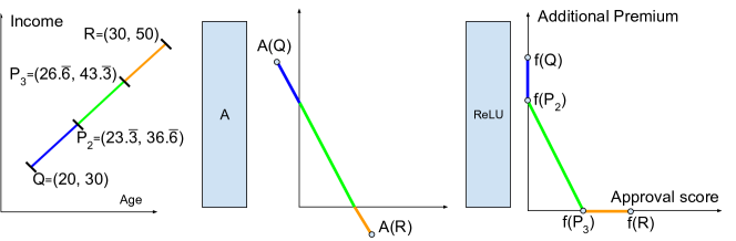
Figure 1: Computing the linear restriction of $f$ (Equation 1) using ExactLine. The input line segment $\overline{QR}$ is divided into three linear partitions such that the transformation from input space to output space (left plot to right plot) is affine (Equation 2). Tick marks (on the left) are used in figures throughout this paper to indicate the partition endpoints $(P_{1},P_{2},\ldots,P_{n})$.

Other Network Analysis Techniques

Compared to prior work, our solution to ExactLine presents an interesting and unique design point in the space of neural-network analysis. Approaches such as [12, 34, 16] are precise, but exponential time because they work over the entire input domain. On another side of the design space, approaches such as those used in [15, 34, 35, 17, 36, 32] are significantly faster while still working over the full-dimensional input space, but accomplish this by trading analysis precision for speed. This trade-off between speed and precision is particularly well-illuminated by [jordan2019provable], which monotonically refines its analysis when given more time. In contrast, the key observation underlying our work is that we can perform both an efficient (worst-case polynomial time for a fixed number of layers) and precise analysis by restricting the input domain to be one dimensional (a line). This insight opens a new dimension to the discussion of network analysis tools, showing that dimensionality can be traded for significant gains in both precision and efficiency (as opposed to prior work which has explored the tradeoff primarily along the precision and efficiency axes under the assumption of high-dimensional input regions). hanin2019complexity similarly considers one-dimensional input spaces, but the paper is focused on a number of theoretical properties and does not focus on the algorithm used in their empirical results.

Algorithm

We will first discuss computation of ExactLine for individual layers. Note that by definition, ExactLine for affine layers does not introduce any new linear partitions. This is captured by Theorem 1 (proved in Appendix D) below:

Theorem 1.

For any affine function $A:X\to Y$ and line segment $\overline{QR}\subset X$, the following is a suitable linear partitioning (Definition 1): $\mathcal{P}\big{(}A{{}_{\restriction{\overline{QR}}}}\big{)}=(Q,R)$.

The following theorem (proved in Appendix E) presents a method of computing $\mathcal{P}\big{(}\mathrm{ReLU}{{}_{\restriction{\overline{QR}}}}\big{)}$.

Theorem 2.

Given a line segment $\overline{QR}$ in $d$ dimensions and a rectified linear layer $\mathrm{ReLU}(x)=(\mathrm{max}(x_{1},0),\ldots,\mathrm{max}(x_{d},0))$, the following is a suitable linear partitioning (Definition 1):

$$\mathcal{P}\big{(}\mathrm{ReLU}{{}_{\restriction{\overline{QR}}}}\big{)}=\mathrm{sorted}\left(\left(\{Q,R\}\cup\{Q+\alpha(R-Q)\mid\alpha\in D\}\right)\cap\overline{QR}\right),$$ (3)

where $D=\left\{-Q_{i}/(R_{i}-Q_{i})\mid 1\leq i\leq d\right\}$, $V_{i}$ is the $i$th component of vector $V$, and $\mathrm{sorted}$ returns a tuple of the points sorted by distance from $Q$.

The essential insight is that we can “follow” the line until an orthant boundary is reached, at which point a new linear region begins. To that end, each number in $D$ represents a ratio between $Q$ and $R$ at which $\overline{QR}$ crosses an orthant boundary. Notably, $D$ actually computes such “crossing ratios” for the unbounded line $\overline{QR}$, hence intersecting the generated endpoints with $\overline{QR}$ in Equation 3.

An analogous algorithm for MaxPool is presented in Appendix F; the intuition is to follow the line until the maximum in any window changes. When a ReLU layer is followed by a MaxPool layer (or vice-versa), the “fused” algorithm described in Appendix G can improve efficiency significantly. More generally, the algorithm described in Appendix H can compute ExactLine for any piecewise-linear function.

Finally, in practice we want to compute $\mathcal{P}\big{(}f{{}_{\restriction{\overline{QR}}}}\big{)}$ for entire neural networks (i.e. sequential compositions of layers), not just individual layers (as we have demonstrated above). The next theorem shows that, as long as one can compute $\mathcal{P}\big{(}L_{i}{{}_{\restriction{\overline{MN}}}}\big{)}$ for each individual layer $L_{i}$ and arbitrary line segment $\overline{MN}$, then these algorithms can be composed to compute $\mathcal{P}\big{(}f{{}_{\restriction{\overline{QR}}}}\big{)}$ for the entire network.

Theorem 3.

Given any piecewise-linear functions $f,g,h$ such that $f=h\circ g$ along with a line segment $\overline{QR}$ where $g(R)\neq g(Q)$ and $\mathcal{P}\big{(}g{{}_{\restriction{\overline{QR}}}}\big{)}=(P_{1},P_{2},\ldots,P_{n})$ is ExactLine applied to $g$ over $\overline{QR}$, the following holds:

$$\mathcal{P}\big{(}f{{}_{\restriction{\overline{QR}}}}\big{)}=\mathrm{sorted}\left(\bigcup_{i=1}^{n-1}{\left\{P_{i}+\frac{y-g(P_{i})}{g(P_{i+1})-g(P_{i})}\times(P_{i+1}-P_{i})\mid y\in\mathcal{P}\big{(}h{{}_{\restriction{\overline{g(P_{i})g(P_{i+1})}}}}\big{)}\right\}}\right)$$

where $\mathrm{sorted}$ returns a tuple of the points sorted by distance from $Q$.

The key insight is that we can first compute ExactLine for the first layer, i.e. $\mathcal{P}\big{(}L_{1}{{}_{\restriction{\overline{QR}}}}\big{)}=(P^{1}_{1},P^{1}_{2},\ldots,P^{1}_{n})$, then we can continue computing ExactLine for the rest of the network within each of the partitions $\overline{P^{1}_{i}P^{1}_{i+1}}$ individually.

In Appendix C we show that, over arbitrarily many affine layers, $l$ ReLU layers each with $d$ units, and $m$ MaxPool or MaxPool + ReLU layers with $w$ windows each of size $s$, at most $\mathrm{O}((d+ws)^{l+m})$ segments may be produced. If only ReLU and affine layers are used, at most $\mathrm{O}(d^{l})$ segments may be produced. Notably, this is a significant improvement over the $\mathrm{O}((2^{d})^{l})$ upper-bound and $\mathrm{\Omega}(l\cdot(2^{d}))$ lower-bound of Xiang et al. [34]. One major reason for our improvement is that we particularly consider one-dimensional input lines as opposed to arbitrary polytopes. Lines represent a particularly efficient special case as they are efficiently representable (by their endpoints) and, being one-dimensional, are not subject to the combinatorial blow-up faced by transforming larger input regions. Furthermore, in practice, we have found that the majority of ReLU nodes are “stable”, and the actual number of segments remains tractable; this algorithm for ExactLine often executes in a matter of seconds for networks with over $60,000$ units (whereas the algorithm of Xiang et al. [34] runs in at least exponential $\mathrm{O}(l\cdot(2^{d}))$ time regardless of the input region as it relies on trivially considering all possible orthants).

3 Characterizing Decision Boundaries for ACAS Xu

Legend:   Clear-of-Conflict,   Weak Right,   Strong Right,   Strong Left,   Weak Left.

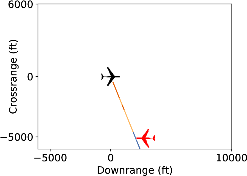
(a) Single line varying $\rho$

(b) Sampling different $\rho$s

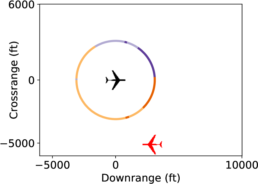
(c) Single line varying $\theta$

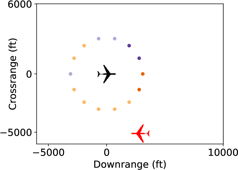
(d) Sampling different $\theta$s

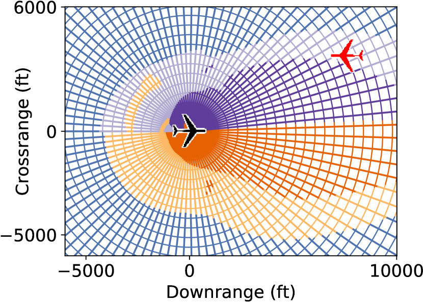
(e) Combination of lines varying $\rho$ and lines varying $\theta$

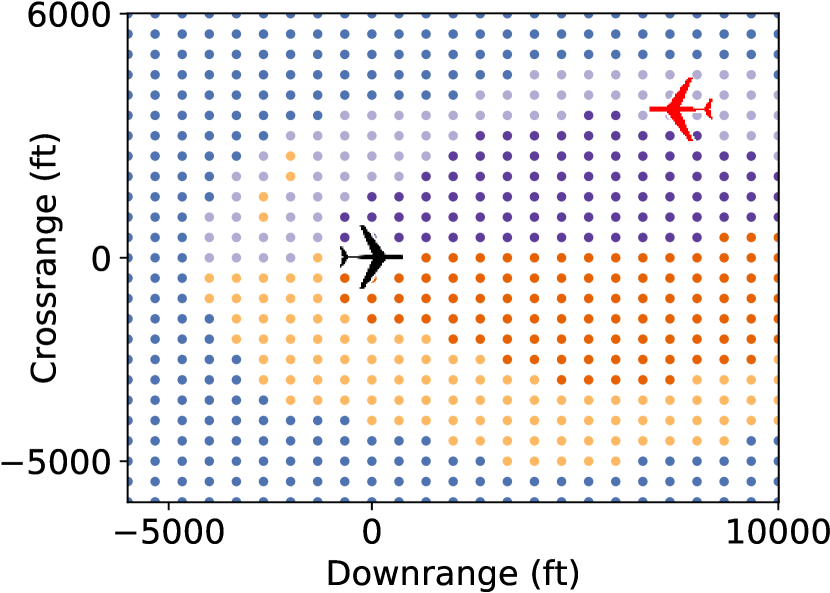
(f) Sampling finitely many points

Figure 2: (a)–(d) Understanding the decision boundary of an ACAS Xu aircraft avoidance network along individual lines using ExactLine ((a), (c)) and finite sampling ((b), (d)). In the ExactLine visualizations there is a clear region of “strong left” in a region that is otherwise “weak left” that does not show in the sampling plots due to the sampling density chosen. In practice, it is not clear what sampling density to choose, thus the resulting plots can be inaccurate and/or misleading. (e)–(f) Computing the decision boundaries among multiple lines and plotting on the same graph. Using ExactLine to sample infinitely many points provides more confidence in the interpretation of the decision boundaries. Compare to similar figures in Julian et al. [5], Katz et al. [12].

The first application of ExactLine we consider is that of understanding the decision boundaries of a neural network over some infinite set of inputs. As a motivating example, we consider the ACAS Xu network trained by Julian et al. [5] to determine what action an aircraft (the “ownship”) should take in order to avoid a collision with an intruder. After training such a network, one usually wishes to probe and visualize the recommendations of the network. This is desirable, for example, to determine at what distance from the ownship an intruder causes the system to suggest a strong change in heading, or to ensure that distance is roughly the same regardless of which side the intruder approaches.

The simplest approach, shown in Figure 2(f) and currently the standard in prior work, is to consider a (finite) set of possible input situations (samples) and see how the network reacts to each of them. This can help one get an overall idea of how the network behaves. For example, in Figure 2(f), we can see that the network has a mostly symmetric output, usually advising the plane to turn away from the intruder when sufficiently close. Although sampling in this way gives human viewers an intuitive and meaningful way of understanding the network’s behavior, it is severely limited because it relies on sampling finitely many points from a (practically) infinite input space. Thus, there is a significant chance that some interesting or dangerous behavior of the network may be exposed with more samples.

By contrast, the ExactLine primitive can be used to exactly determine the output of the network at all of the infinitely many points on a line in the input region. For example, in Figure 2(a), we have used ExactLine to visualize a particular head-on collision scenario where we vary the distance of the intruder (specified in polar coordinates $(\rho,\theta)$) with respect to the ownship (always at $(0,0)$). Notably, there is a region of “Strong Left” in a region of the line that is otherwise entirely “Weak Left“ that shows up in Figure 2(a) (the ExactLine method) but not in Figure 2(b) (the sampling method). We can do this for lines varying the $\theta$ parameter instead of $\rho$, result in Figure 2(c) and Figure 2(d). Finally, repeating this process for many lines and overlapping them on the same graph produces a detailed “grid” as shown in Figure 2(e).

Figure 2(e) also shows a number of interesting and potentially dangerous behaviors. For example, there is a significant region behind the plane where an intruder on the left may cause the ownship to make a weak left turn towards the intruder, an unexpected and asymmetric behavior. Furthermore, there are clear regions of strong left/right where the network otherwise advises weak left/right. Meanwhile, in Figure 2(f), we see that the sampling density used is too low to notice the majority of this behavior. In practice, it is not clear what sampling density should be taken to ensure all potentially-dangerous behaviors are caught, which is unacceptable for safety-critical systems such as aircraft collision avoidance.

Takeaways. ExactLine can be used to visualize the network’s output on infinite subsets of the input space, significantly improving the confidence one can have in the resulting visualization and in the safety and accuracy of the model being visualized.

Future Work. One particular area of future work in this direction is using ExactLine to assist in network verification tools such as Katz et al. [12] and Gehr et al. [15]. For example, the relatively-fast ExactLine could be used to check infinite subsets of the input space for counter-examples (which can then be returned immediately) before calling the more-expensive complete verification tools.

4 Exact Computation of Integrated Gradients

Integrated Gradients (IG) [25] is a method of attributing the prediction of a DNN to its input features. Suppose function $F:\mathbb{R}^{n}\to[0,1]$ defines the network. The integrated gradient along the $i^{th}$ dimension for an input $x=(x_{1},\ldots,x_{n})\in\mathbb{R}^{n}$ and baseline $x^{\prime}\in\mathbb{R}^{n}$ is defined as:

$$\small IG_{i}(x)\buildrel\mbox{\tiny{def}}\over{=}(x_{i}-x_{i}^{\prime})\times\int_{\alpha=0}^{1}\frac{\partial F(x^{\prime}+\alpha\times(x-x^{\prime}))}{\partial x_{i}}d\alpha$$ (4)

Thus, the integrated gradient along all input dimensions is the integral of the gradient computed on all points on the straightline path from the baseline $x^{\prime}$ to the input $x$. In prior work it was not known how to exactly compute this integral for complex networks, so it was approximated using the left-Riemann summation of the gradients at $m$ uniformly sampled points along the straightline path from $x^{\prime}$ to $x$:

$$\small\widetilde{IG}_{i}^{m}\buildrel\mbox{\tiny{def}}\over{=}(x_{i}-x_{i}^{\prime})\times\sum_{0\leq k<m}\frac{\partial F(x^{\prime}+\frac{k}{m}\times(x-x^{\prime}))}{\partial x_{i}}\times\frac{1}{m}$$ (5)

The number of samples $m$ determines the quality of this approximation. Let $\widetilde{m}$ denote the number of samples that is large enough to ensure that $\sum_{i=1}^{n}\widetilde{IG}_{i}^{\widetilde{m}}\approx F(x)-F(x^{\prime})$. This is the recommended number of samples suggested by Sundararajan et al. [25]. In practice, $\widetilde{m}$ can range between 20 and 1000 [25, 37].

While the (exact) IG described by Equation 4 satisfies properties such as completeness [25, §3] and sensitivity [25, §2.1], the approximation computed in practice using Equation 5 need not.

Figure 3: “Integrated Gradients” is a powerful method of neural network attribution. IG relies on computing the integral of the gradients of the network at all points linearly interpolated between two images (as shown above), however previous work has only been able to approximate the true IG, casting uncertainty on the results. Within each partition identified by ExactLine (delineated by vertical lines) the gradient is constant, so computing the exact IG is possible for the first time.

The integral in Equation 4 can be computed exactly by adding an additional condition to the definition of ExactLine: that the gradient of the network within each partition is constant. It turns out that this stricter definition is met by all of the algorithms we have discussed so far, a fact we discuss in more detail in Appendix J. For ReLU layers, for example, because the network acts like a single affine map within each orthant, and we split the line such that each partition is entirely contained within an orthant, the network’s gradient is constant within each orthant (and thus along each ExactLine partition). This is stated formally by Theorem 4 and proved in Appendix J:

Theorem 4.

For any network $f$ with nonlinearities introduced only by ReLU functions and $\mathcal{P}\big{(}f{{}_{\restriction{\overline{QR}}}}\big{)}=(P_{1},P_{2},\ldots,P_{n})$ computed according to Equation 3, the gradient of $f$ with respect to its input vector $x$, i.e. $\nabla f(x)$, is constant within each linear partition $\overline{P_{i}P_{i+1}}$.

This allows us to exactly compute the IG of each individual partition $r$ ($RIG^{r}_{i}$) by finding the gradient at any point in that partition and multiplying by the width of the partition:

$$\small RIG^{r}_{i}(x)\buildrel\mbox{\tiny{def}}\over{=}(P_{(r+1)i}-P_{ri})\times\frac{\partial F(0.5\times(P_{ri}+P_{(r+1)i}))}{\partial x_{i}}$$ (6)

Compared to Equation 4, Equation 6 computes the IG for partition for $\overline{P_{r}P_{r+1}}$ by replacing the integral with a single term (arbitrarily choosing $\alpha=0.5$, i.e. the midpoint) because the gradient is uniform along $\overline{P_{r}P_{r+1}}$. The exact IG of $\overline{x^{\prime}x}$ is the sum of the IGs of each partition:

$$\small IG_{i}(x)=\sum_{r=1}^{n}RIG^{r}_{i}(x)$$ (7)

Table 1: Mean relative error for approximate IG (using $\widetilde{m}$) compared to exact IG (using ExactLine) on CIFAR10. The approximation error is surprisingly high.

	Error (%)
convsmall	24.95
convmedium	24.05
convbig	45.34

Table 2: Average number of samples needed by different IG approximations to reach $5\%$ relative error w.r.t. exact IG (using ExactLine). Outliers requiring over $1,000$ samples were not considered. Using trapezoidal rule instead of a left-sum can cause large gains in accuracy and performance.

	Exact	Approximate
		left	right	trap.
convsmall	2582.74	136.74	139.40	91.67
convmedium	3578.89	150.31	147.59	91.57
convbig	14064.65	269.43	278.20	222.79

Empirical Results. A prime interest of ours was to determine the accuracy of the existing sampling method. On three different CIFAR10 networks [ERAN], we took each image in the test set and computed the exact IG against a black baseline using Equation 7. We then found $\widetilde{m}$ and computed the mean relative error between the exact IG and the approximate one. As shown in Table 2, the approximate IG has an error of $25-45\%$. This is a concerning result, indicating that the existing use of IG in practice may be misleading. Notably, without ExactLine, there would be no way of realizing this issue, as this analysis relies on computing the exact IG to compare with.

For many smaller networks considered, we have found that computing the exact IG is relatively fast (i.e., at most a few seconds) and would recommend doing so for situations where it is feasible. However, in some cases the number of gradients that would have to be taken to compute exact IG is high (see Column 2, Table 2). In such cases, we can use our exact computation to understand how many uniform samples one should use to compute the approximate IG to within $5\%$ of the exact IG. To that end, we performed a second experiment by increasing the number of samples taken until the approximate IG reached within $5\%$ error of the exact IG. In practice, we found there were a number of “lucky guess” situations where taking, for example, exactly $5$ samples led to very high accuracy, but taking $4$ or $6$ resulted in very poor accuracy. To minimize the impact of such outliers, we also require that the result is within $5\%$ relative error when taking up to $5$ more samples. In Table 2 the results of this experiment are shown under the column “left,” where it becomes clear that relatively few samples (compared to the number of actual linear regions under “exact”) are actually needed. Thus, one can use ExactLine on a test set to understand how many samples are needed on average to get within a desired accuracy, then use that many samples when approximating IG.

Finally, the left Riemann sum used by existing work in IG [25] is only one of many possible sampling methods; one could also use a right Riemann sum or the “Trapezoidal Rule.” With ExactLine we can compute the exact IG and quantify how much better or worse each approximation method is. To that end, the columns “right” and “trap.” in Table 2 show the number of samples one must take to get consistently within $5\%$ of the exact integrated gradients. Our results show the number of samples needed to accurately approximate IG with trapezoidal rule is significantly less than using left and right sums. Note that, because these networks are piecewise-linear functions, it is possible for trapezoidal sampling to be worse than left or right sampling, and in fact for all tested models there were images where trapezoidal sampling was less accurate than left and right sampling. This is why having the ability to compute the exact IG is important, to ensure that we can empirically quantify the error involved in and justify choices between different heuristics. Furthermore, we find a per-image reduction in the number of samples needed of $20-40\%$ on average. Thus, we also recommend that users of IG use a trapezoidal approximation instead of the currently-standard left sum.

Takeaways. ExactLine is the first method for exactly computing integrated gradients, as all other uses of the technique have sampled according to Equation 5. From our results, we provide two suggestions to practitioners looking to use IG: (1) Use ExactLine on a test set before deployment to better understand how the number of samples taken relates to approximation error, then choose sampling densities at runtime based on those statistics and the desired accuracy; (2) Use the trapezoidal rule approximation when approximating to get better accuracy with fewer samples.

Future Work. ExactLine can be used to design new IG approximation using non-uniform sampling. ExactLine can similarly be used to exactly compute other measures involving path integrals such as neuron conductance [39], a refinement of integrated gradients.

5 Understanding Adversarial Examples

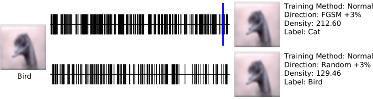
Figure 4: Comparing the density of linear partitions from a test image to FGSM and random baselines. The long blue line segment indicates the change in classification. (1) Even within a small perturbation of the input point, there is significant non-linear behavior in the network. (2) Although the linear hypothesis for adversarial examples predicts that both normal inputs and their corresponding adversarial examples (“FGSM + 3%”) will lie on the same linear region, we find in practice that, not only do they lie on different linear regions, but there is significantly more non-linearity in the adversarial (FGSM) direction than a random direction. This falsifies the fundamental assumption behind the linear explanation of adversarial examples.

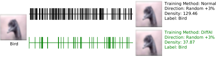
Figure 5: Comparing the density of linear partitions from a test image to random baselines for normal (in black) and DiffAI-protected networks (in green). Networks trained with the DiffAI robust-training scheme tend to exhibit significantly fewer non-linearities than their normally-trained counterparts.

We use ExactLine to empirically investigate and falsify a fundamental assumption behind a well-known hypothesis for the existence of adversarial examples. In the process, using ExactLine, we discover a strong association between robustness and the empirical linearity of a network, which we believe may help spur future work in understanding the source of adversarial examples.

Empirically Testing the Linear Explanation of Adversarial Examples. We consider in this section one of the dominant hypotheses for the problem of adversarial examples ([6, 7, 8]), first proposed by Goodfellow et al. [7] and termed the “Linear Explanation of Adversarial Examples.” It makes a fundamental assumption that, when restricted to the region around a particular input point, the output of the neural network network is linear, i.e. the tangent plane to the network’s output at that point exactly matches the network’s true output. Starting from this assumption, Goodfellow et al. [7] makes a theoretical argument concluding that the phenomenon of adversarial examples results from the network being “too linear.” Although theoretical debate has ensued as to the merits of this argument [40], the effectiveness of adversarials generated according to this hypothesis (i.e., using the standard “fast gradient sign method” or “FGSM”) has sustained it as one of the most well-subscribed-to theories as to the source of adversarial examples. However, to our knowledge, the fundamental assumption of the theory—that real images and their adversarial counterparts lie on the same linear region of a neural network—has not been rigorously validated empirically.

Table 3: Density of FGSM line partitions divided by density of Random line partitions. FGSM directions tend to be significantly more dense than random directions, contradicting the well-known Linear Explanation of Adversarial Examples. Mdn: Median, 25%: 25% percentile, 75%: 75% percentile

(a) MNIST

	FGSM/Random
Training Method	Mdn	25%	75%
Normal	1.36	0.99	1.76
DiffAI	0.98	0.92	1.38
PGD	1.22	0.97	1.51

(b) CIFAR10

	FGSM/Random
Training Method	Mdn	25%	75%
Normal	1.78	1.60	2.02
DiffAI	1.67	1.47	2.03
PGD	1.84	1.65	2.10

To empirically validate this hypothesis, we looked at the line between an image and its FGSM-perturbed counterpart (which is classified differently by the network), then used ExactLine to quantify the density of each line (the number of linear partitions — each delineated by tick marks in Figure 4 — divided by the distance between the endpoints). If the underlying linearity assumption holds, we would expect that both the real image and the perturbed image lie on the same linear partition, thus we would not expect to see the line between them pass through any other linear partitions. In fact (top of Figure 4), we find that the adversarial image seems to lie across many linear partitions, directly contradicting the fundamental assumption of Goodfellow et al. [7]. We also compared this line to the line between the real image and the real image randomly perturbed by the same amount (bottom of Figure 4). As shown in Table 3(b), the FGSM direction seems to pass through significantly more linear partitions than a randomly chosen direction. This result shows that, not only is the linearity assumption not met, but in fact the opposite appears to be true: adversarial examples are associated with unusually non-linear directions of the network.

With these results in mind, we realized that the linearity assumption as initially presented in Goodfellow et al. [7] is stronger than necessary; it need only be the case that the gradient is reasonably constant across the line, so that the tangent plane approximation used is still reasonably accurate. To measure how well the tangent plane approximates the function between normal and adversarial inputs, we compared the gradient taken at the real image (i.e., used by FGSM) to the gradients at each of the intermediate linear partitions, finding the mean error between each and averaging weighted by size of the partition. If this number is near $0$, it implies that, although many theoretically distinct linear partitions exist between the two points, they have roughly the same “slope” and thus the tangent plane approximation would be accurate and the Linearity Hypothesis may still be a worthwhile explanation of the phenomenon of adversarial examples. However, we find that this number is larger than $250\%$ when averaged over all images tested, implying that the tangent plane is not a particularly good approximation of the underlying function in these regions of input space and providing further empirical evidence against the Linear Explanation of adversarial examples.

Table 4: Comparing density of lines when different training algorithms (normal, DiffAI, and PGD) are used. We report the mean of those ratios across all tested lines. These results indicate that networks trained to be adversarially robust with DiffAI or PGD training methods tend to behave more linearly than non-robust models. Mdn: Median, 25%: 25% percentile, 75%: 75% percentile

(a) MNIST

	Normal/DiffAI				Normal/PGD
Dir.	Mdn	25%	75%		Mdn	25%	75%
FGSM	3.05	2.05	4.11		0.88	0.66	1.14
Rand.	2.50	1.67	3.00		0.80	0.62	1.00

(b) CIFAR10

	Normal/DiffAI				Normal/PGD
Dir.	Mdn	25%	75%		Mdn	25%	75%
FGSM	3.37	2.77	4.94		1.48	1.22	1.67
Rand.	3.43	2.78	4.42		1.51	1.21	1.80

Characteristics of Adversarially-Trained Networks. We also noticed an unexpected trend in the previous experiment: networks trained to be robust to adversarial perturbations (particularly DiffAI-trained networks [33]) seemed to have significantly fewer linear partitions in all of the lines that we evaluated them on (see Figure 5). Further experiments, summarized in Table 4(b), showed that networks trained to be adversarially robust with PGD and especially DiffAI training methods exhibit up to $5\times$ fewer linear partitions for the same change in input. This observation suggests that the neighborhoods around points in adversarially-trained networks are “flat” (more linear).

Takeaways. Our results falsify the fundamental assumption behind the well-known Linear Explanation for adversarial examples. Adversarial training tends to make networks more linear.

Future Work. ExactLine can be used to investigate adversarial robustness. Further investigation into why DiffAI-protected networks tend to be more linear will help resolve the question (raised in this work) of whether reduced density of linear partitions contributes to robustness, or increased robustness results in fewer linear partitions (or if there is a third important variable impacting both).

6 Conclusion

We address the problem of computing a succinct representation of a linear restriction of a neural network. We presented ExactLine, a novel primitive for the analysis of piecewise-linear deep neural networks. Our algorithm runs in a matter of a few seconds on large convolutional and ReLU networks, including ACAS Xu, MNIST, and CIFAR10. This allows us to investigate questions about these networks, both shedding new light and raising new questions about their behavior.

Acknowledgements

We thank Nina Amenta, Yong Jae Lee, Cindy Rubio-González, and Mukund Sundararajan for their feedback and suggestions on this work. This material is based upon work supported by AWS Cloud Credits for Research.

Computing Linear Restrictions of Neural Networks: Supplemental

Appendix A Specification of Evaluation Hardware

Although we do not claim particular performance results, we do point out that all ExactLine uses in our experiments took only a matter of seconds on commodity hardware (although in some cases the experiments themselves took a few minutes, particularly when computing gradients for Section 4).

For reproducibility, all experimental data reported was run on Amazon EC2 c5.metal instances, using BenchExec [benchexec] to limit to 16 CPU cores and 16 GB of memory. We have also run the results on commodity hardware, namely an Intel Core i7-7820X CPU at 3.6GHz with 32GB of memory (both resources shared with others simultaneously), for which the “matter of seconds” characterization above holds as well.

All experiments were only run on CPU, although we believe computing ExactLine on GPUs is an important direction for future research on significantly larger networks.

Appendix B Uniqueness of ExactLine

The smallest tuple satisfying the requirements on $\mathcal{P}\big{(}f{{}_{\restriction{\overline{QR}}}}\big{)}$ is unique (when it exists) for any given $f$ and $QR$, and any tuple satisfying $\mathcal{P}\big{(}f{{}_{\restriction{\overline{QR}}}}\big{)}$ can be converted to this minimal tuple by removing any endpoint $P_{i}$ which lies on $\overline{P_{i-1}P_{i+1}}$. In the proceeding text we will discuss methods for computing some tuple satisfying $\mathcal{P}\big{(}f{{}_{\restriction{\overline{QR}}}}\big{)}$; if the reader desires, they can use the procedure mentioned in the previous sentence to reduce this to the unique smallest such tuple. However, we note that the algorithms below usually produce the minimal tuple on real-world networks even without any reduction procedure due to the high dimensionality of the functions involved.

Appendix C Runtime of ExactLine Algorithms

We note that the algorithm corresponding to Theorem 1 runs on a single line segment in constant time producing a single resulting line segment. The algorithm corresponding to Equation 3 runs on a single line segment in $\mathrm{O}(d)$ time, producing at most $\mathrm{O}(d)$ new segments. If $w$ is the number of windows and $s$ is the size of each window, the algorithms for MaxPool and ReLU + MaxPool run in time $\mathrm{O}(ws^{2})$ and produce $\mathrm{O}(ws)$ new line segments. Thus, using the algorithm corresponding to Theorem 3, over arbitrarily many affine layers, $l$ ReLU layers each with $d$ units, and $m$ MaxPool or MaxPool + ReLU layers with $w$ windows each of size $s$, then at most $\mathrm{O}((d+ws)^{l+m})$ segments may be produced. If only $l$ ReLU and arbitrarily-many affine layers are used, at most $\mathrm{O}(d^{l})$ segments may be produced.

Appendix D ExactLine for Affine Layers

See 1

Proof.

By the definition of $\mathcal{P}\big{(}A{{}_{\restriction{\overline{QR}}}}\big{)}$ it suffices to show that $\{\overline{QR}\}$ partitions $\overline{QR}$ and produce an affine map $A^{\prime}$ such that $A(x)=A^{\prime}(x)$ for every $x\in\overline{QR}$.

The first fact follows directly, as $\overline{QR}=\overline{QR}\implies\overline{QR}\subseteq\overline{QR}$ and every element of $\overline{QR}$ belongs to $\overline{QR}$.

For the second requirement, we claim that $A^{\prime}=A$ satisfies the desired property, as $A$ is affine and $A(x)=A(x)$ for all $x$ in general and in particular for all $x\in\overline{QR}$. ∎

Appendix E ExactLine for ReLU Layers

See 2

Proof.

First, we define the ReLU function like so:

$$\begin{bmatrix}\delta_{1\mathrm{sign}(x_{1})}&0&\cdots&0\\ 0&\delta_{1\mathrm{sign}(x_{2})}&\cdots&0\\ \vdots&\vdots&\ddots&\vdots\\ 0&0&\cdots&\delta_{1\mathrm{sign}(x_{d})}\\ \end{bmatrix}\begin{bmatrix}x_{1}\\ x_{2}\\ \vdots\\ x_{d}\end{bmatrix}$$

where $\mathrm{sign}(x)$ returns $1$ if $x$ is positive and $0$ otherwise while $\delta_{ij}$ is the Kronecker delta.

Now, it becomes clear that, as long as the signs of each $x_{i}$ are constant, the ReLU function is linear.

We note that, over a Euclidean line segment $\overline{QR}$, we can parameterize $\overline{QR}$ as $\overline{QR}(\alpha)=Q+\alpha(R-Q)$. Considering the $i$th component, we have a linear relation $\overline{QR}_{i}(\alpha)=Q_{i}+\alpha(R_{i}-Q_{i})$ which changes sign at most once, when $\overline{QR}_{i}(\alpha)=0$ (because linear functions in $\mathbb{R}$ are continuous and monotonic). Thus, we can solve for the sign change of the $i$th dimension as:

$$\overline{QR}_{i}(\alpha)=0$$

$$\implies 0=Q_{i}+\alpha(R_{i}-Q_{i})$$

$$\implies \alpha=-\frac{Q_{i}}{R_{i}-Q_{i}}$$

As we have restricted the function to $0\leq\alpha\leq 1$, at any $\alpha$ within these bounds the sign of some component changes and the function acts non-linearly. Between any two such $\alpha$s, however, the signs of all components are constant, so the ReLU function is perfectly described by a linear map as shown above. Finally, we can solve for the endpoints corresponding to any such $\alpha$ using the parameterization $\overline{QR}(\alpha)$ defined above, resulting in the formula in the theorem.

$Q,R$ are included to meet the partitioning definition, as the sign of some element may not be $0$ at the $Q,R$ endpoints. ∎

Appendix F ExactLine for MaxPool Layers

As discussed in the paper, although we do not use MaxPool layers in any of our evaluated networks, we have developed and implemented an algorithm for computing $\mathcal{P}\big{(}\mathrm{MaxPool}{{}_{\restriction{\overline{QR}}}}\big{)}$, which we present here. In particular, we present $\mathcal{P}\big{(}\mathrm{MaxPoolWindow}{{}_{\restriction{\overline{QR}}}}\big{)}$, i.e. the linear restriction for any given window. $\mathcal{P}\big{(}\mathrm{MaxPool}{{}_{\restriction{\overline{MN}}}}\big{)}$ can be then be computed by separating each window $\overline{QR}$ from $\overline{MN}$ and applying $\mathcal{P}\big{(}\mathrm{MaxPoolWindow}{{}_{\restriction{\overline{QR}}}}\big{)}$. Notably, there may be duplicate endpoints (e.g. if there is overlap in the windows) which can be handled by removing duplicates if desired.

Input: $\overline{QR}$, the line segment to restrict the MaxPoolWindow function to.

Output: $\mathcal{P}\big{(}\mathrm{MaxPoolWindow}{{}_{\restriction{\overline{QR}}}}\big{)}$

$\mathcal{P}\leftarrow[Q]$

 // Begin an (ordered) list of points with one item, $Q$.

$\alpha\leftarrow 0.0$

 // Ratio along $\overline{QR}$ of the last endpoint in $\mathcal{P}$.

$m\leftarrow\mathrm{argmax}(Q)$

 // Maximum component of the last endpoint in $\mathcal{P}$.

1 while $m\neq\mathrm{argmax}(R)$ do

2       $D\leftarrow\frac{Q-Q_{m}}{(R_{i}-Q_{i})-(R-Q)}$

3       $A\leftarrow\{(D_{i},i)\mid 1\leq i\leq d\wedge\alpha<D_{i}<1.0\}$

4       if $A=\emptyset$ then  break

       $(\alpha,m)\leftarrow\mathrm{lexmin}(A)$

       // Lexicographical minimum of the tuples in $A$.

5       $\mathrm{append}(\mathcal{P},Q+\alpha\times(R-Q))$

6      

7$\mathrm{append}(\mathcal{P},R)$

return $\mathcal{P}$

 // Interpret the list $\mathcal{P}$ as a tuple and return it.

Algorithm 1 $\mathcal{P}\big{(}\mathrm{MaxPoolWindow}{{}_{\restriction{\overline{QR}}}}\big{)}$. Binary operations involving both scalars and vectors apply the operation element-wise to each component of the vector.

Proof.

MaxPool applies a separate mapping from each input window to each output component, so it suffices to consider each window separately.

Within a given window, the MaxPool operation returns the value of the maximum component. It is thus linear while the index of the maximum component remains constant. Now, we parameterize $\overline{QR}(\alpha)=Q+\alpha\times(R-Q)$. At each iteration of the loop we solve for the next point at which the maximum index changes. Assuming the maximum index is $m$ when $\alpha=\alpha_{m}$, we can solve for the next ratio $\alpha_{i}>\alpha_{m}$ at which index $i$ will become larger than $m$ like so (again realizing that linear functions are monotonic):

$$\overline{QR}_{m}(\alpha_{i})=\overline{QR}_{i}(\alpha_{i})$$

$$\implies Q_{m}+\alpha_{i}\times(R_{m}-Q_{m})=Q_{i}+\alpha_{i}\times(R_{i}-Q_{i})$$

$$\implies \alpha_{i}\times(R_{m}-Q_{m}+Q_{i}-R_{i})=Q_{i}-Q_{m}$$

$$\implies \alpha_{i}=\frac{Q_{i}-Q_{m}}{(R_{m}-Q_{m})+Q_{i}-R_{i}}$$

If $\alpha_{m}\leq\alpha_{i}<1$, then component $i$ becomes larger than component $m$ at $\overline{QR}(\alpha_{i})$. We can compute this for all other indices (producing set $A$ in the algorithm) then find the first index that becomes larger than $m$. We assign this index to $m$ and its ratio to $\alpha$. If no such index exists, we can conclude that $m$ remains the maximum until $R$, thus additional endpoints are not needed.

Thus, within any two points in $P$ the maximum component stays the same, so the MaxPool can be exactly replaced with a linear map returning only that maximum element. ∎

At worst, then, for each of the $w$ windows each of size $s$, we may add $O(s)$ new endpoints ($\overline{QR}(\alpha)$ is monotonic in each component so the maximum index can only change $s$ times), and for each of those $O(s)$ new endpoints we must re-compute $D$, which requires $\mathrm{O}(s)$ operations. Thus, the time complexity for each window is $\mathrm{O}(s^{2})$ and for the entire MaxPool computation is $\mathrm{O}(ws^{2})$.

Although most practical applications (especially on medium-sized networks) do not reach that worst-case bound, on extremely large (ImageNet-sized) networks we have found that such MaxPool computations end up taking the majority of the computation time. We believe this is an area for future work, perhaps using GPUs or other deep-learning hardware to perform the analysis.

Appendix G ExactLine for MaxPool + ReLU Layers

When a MaxPool layer is followed by a ReLU layer (or vice-versa), the preceding algorithm may include a large number of unnecessary points (for example, if the maximum index changes but the actual value remains less than $0$, the ReLU layer will ensure that both pieces of the MaxPool output are mapped to the same constant value $0$). To avoid this, the MaxPool algorithm above can be modified to check before adding each $P_{i}$ whether the value at the maximum index is below $0$ and thus avoid adding unnecessary points. This can be made slightly more efficient by “skipping” straight to the first index where the value becomes positive, but overall the worst-case time complexity remains $\mathrm{O}(ws^{2})$.

Appendix H ExactLine for General Piecewise-Linear Layers

A more general algorithm can be devised for any piecewise-linear layer, as long as the input space can be partitioned into finitely-many (possibly unbounded) convex polytopes, where the function is affine within each one. For example, ReLU fits this definition where the convex polytopes are the orthants. Once this has been established, then, we take the union of the hyperplanes defining the faces of each convex polytope. In the ReLU example, each convex polytope defining the linear regions corresponds to a single orthant. Each orthant has an “H-representation” in the form $\{x\mid x_{1}\leq 0\wedge x_{2}>0\wedge\ldots\wedge x_{n}\leq 0\}$, where we say the corresponding “hyperplanes defining the faces” of this polytope are $\{\{x\mid x_{1}=0\},\ldots,\{x\mid x_{n}=0\}\}$ (i.e., replacing the inequalities in the conjunction with equalities). Finally, given line segment $\overline{QR}$, we compare $Q$ and $R$ to each hyperplane individually; wherever $Q$ and $R$ lie on opposite sides of the hyperplane, we add the intersection point of the hyperplane with $\overline{QR}$. Sorting the resulting points gives us a valid $\mathcal{P}\big{(}f{{}_{\restriction{\overline{QR}}}}\big{)}$ tuple. If desired, the minimization described in Section 2 can be applied to recover the unique smallest $\mathcal{P}\big{(}f{{}_{\restriction{\overline{QR}}}}\big{)}$ tuple.

The intuition behind this algorithm is exactly the same as that behind the ReLU algorithm; partition the line such that each resulting segment lies entirely within a single one of the polytopes. The further intuition here is that, if a point lies on a particular side of all of the faces defining the set of polytopes, then it must lie entirely within a single one of those polytopes (assuming the polytopes partition the input space).

Note that this algorithm can also be used to compute ExactLine for MaxPool layers, however, in comparison, the algorithm in Appendix F effectively adds two optimizations. First, the “search space” of possibly-intersected faces at any point is restricted to only the faces of the polytope that the last-added point resides in (minimizing redundancy and computation needed). Second, we always add the first (i.e., closest to $Q$) intersection found, so we do not have to sort the points at the end (we literally “follow the line”). Such function-specific optimizations tend to be beneficial when the partitioning of the input space is more complex (eg. MaxPool); for component-wise functions like ReLU, the general algorithm presented above is extremely efficient.

Appendix I ExactLine Over Multiple Layers

Here we prove Theorem 3, which formalizes the intuition that we can solve ExactLine for an entire piecewise-linear network by solving it for all of the intermediate layers individually. Then, we use ExactLine on each layer in sequence, with each layer partitioning the input line segment further so that ExactLine on each latter layer can be computed on each of those partitions.

See 3

Proof.

Consider any linear partition of $g$ defined by endpoints $(P_{i},P_{i+1})$ of $\overline{QR}$. By the definition of $\mathcal{P}\big{(}g{{}_{\restriction{\overline{QR}}}}\big{)}$, there exists some affine map $A_{i}$ such that $g(x)=A_{i}(x)$ for any $x\in\overline{P_{i}P_{i+1}}$.

Now, consider $\mathcal{P}\big{(}h{{}_{\restriction{\overline{g(P_{i})g(P_{i+1})}}}}\big{)}=(O^{i}_{1}=P_{i},O^{i}_{2},\ldots,O^{i}_{m}=P_{i+1})$. By the definition of $\mathcal{P}\big{(}h{{}_{\restriction{\overline{g(P_{i})g(P_{i+1})}}}}\big{)}$, then, for any partition $\overline{O^{i}_{j}O^{i}_{j+1}}$, there exists some affine map $B^{i}_{j}$ such that $h(x)=B^{i}_{j}(x)$ for all $x\in\overline{O^{i}_{j}O^{i}_{j+1}}$.

Realizing that $O^{i}_{j},O^{i}_{j+1}\in\overline{g(P_{i})g(P_{i+1})}$ and that $\overline{P_{i}P_{i+1}}$ maps to $\overline{g(P_{i})g(P_{i+1})}$ under $g$ (affineness of $g$ over $\overline{P_{i}P_{i+1}}$), and assuming $g(P_{i})\neq g(P_{i+1})$ (i.e., $A_{i}$ is non-degenerate), there exist unique $I^{i}_{j},I^{i}_{j+1}\in\overline{P_{i}P_{i+1}}$ such that $g(I^{i}_{j})=O^{i}_{j}$ and $g(I^{i}_{j+1})=O^{i}_{j+1}$. In particular, as affine maps retain ratios along lines, we have that:

$$I^{i}_{j}=P_{i}+\frac{O^{i}_{j}-g(P_{i})}{g(P_{i+1})-g(P_{i})}\times(P_{i+1}-P_{i})$$

And similar for $I^{i}_{j+1}$. (In the degenerate case, we can take $I^{i}_{j}=P_{i},I^{i}_{j+1}=P_{i+1}$ to maintain the partitioning).

Now, we consider the line segment $\overline{I^{i}_{j}I^{i}_{j+1}}\subseteq\overline{P_{i}P_{i+1}}$. As it is a subset of $\overline{P_{i}P_{i+1}}$, all points $x\in\overline{I^{i}_{j}I^{i}_{j+1}}$ are transformed to $A_{i}(x)\in\overline{g(O^{i}_{j})g(O^{i}_{j+1})}$ by $g$. Thus, the application of $h$ to any such point $y=A_{i}(x)\in\overline{O^{i}_{j}O^{i}_{j+1}}$ is $B^{i}_{j}(y)$, and the composition $(B^{i}_{j}\circ A_{i})(x)$ is an affine map taking points $x\in\overline{I^{i}_{j}I^{i}_{j+1}}$ to $f(x)$.

Finally, as the $O_{j}$s partition each $\overline{g(P_{i})g(P_{i+1})}$ and each $\overline{P_{i}P_{i+1}}$ partitions $\overline{QR}$, and we picked $I^{i}_{j}$s to partition each $\overline{P_{i}P_{i+1}}$, the set of $I^{i}_{j}$s partitions $\overline{QR}$. ∎

This theorem can be applied for each layer in a network, allowing us to identify a linear partitioning for the entire network with only linear partitioning algorithms for each individual layer.

Appendix J Constant Gradients with ExactLine

In Section 4, we relied on the fact that the gradients are constant within any linear partition given by $\mathcal{P}\big{(}\textsc{ReLU}{{}_{\restriction{\overline{QR}}}}\big{)}$ computed with Equation 3. This fact was formalized by Theorem 4, which we prove below:

See 4

Proof.

We first notice that the gradient of the entire network, when it is well-defined, is determined completely by the signs of the internal activations (as they control the action of the ReLU function).

Thus, as long as the signs of the internal activations are constant, the gradient will be constant as well.

Equation 4 in our paper identifies partitions where the signs of the internal activations are constant. Therefore, the gradient in each of those regions $\overline{P_{i}P_{i+1}}$ is also constant. ∎

However, in general, for arbitrary $f$, it is possible that the action of $f$ may be affine over the line segment $\overline{P_{i}P_{i+1}}$ but not affine (or not describable by a single $A_{i}$) when considering points arbitrarily close to (but not lying on) $\overline{P_{i}P_{i+1}}$. In other words, the definition of $\mathcal{P}\big{(}f{{}_{\restriction{\overline{QR}}}}\big{)}$ as presented in our paper only requires that the directional derivative in the direction of $\overline{QR}$ is constant within each linear partition $\overline{P_{i}P_{i+1}}$, not the gradient more generally. A stronger definition of ExactLine could integrate such a requirement, but we present the weaker, more-general definition in the text for clarity of exposition.

However, as demonstrated in the above theorem, this stronger requirement is met by Equation 3, thus our exact computation of Integrated Gradients is correct.

Appendix K Further ExactLine Implementation Details

We implemented our algorithms for computing $\mathcal{P}\big{(}f{{}_{\restriction{\overline{QR}}}}\big{)}$ in C++ using a gRPC server with Protobuf interface. This server can be called by a fully-fledged Python interface which allows one to define or import networks from ONNX [41] or ERAN [ERAN] formats and compute $\mathcal{P}\big{(}f{{}_{\restriction{\overline{QR}}}}\big{)}$ for them. For the ACAS Xu experiments, we converted the ACAS Xu models provided in the ReluPlex [12] repository to ERAN format for analysis by our tool.

Internally, we represent $\mathcal{P}\big{(}f{{}_{\restriction{\overline{QR}}}}\big{)}$ by a vector of endpoints, each with a ratio along $\overline{QR}$ (i.e., $\alpha$ for the parameterization $\overline{QR}(\alpha)=Q+\alpha\times(R-Q)$), the layer at which the endpoint was introduced, and the corresponding post-image after applying $f$ (or however many layers have been applied so far).

On extremely large (ImageNet-sized) networks, storing the internal network activations corresponding to each of the thousands of endpoints requires significant memory usage (often hundreds of gigabytes), so our implementation sub-divides $\overline{QR}$ when necessary to control memory usage. However, for all tested networks, our implementation was extremely fast and could compute $\mathcal{P}\big{(}f{{}_{\restriction{\overline{QR}}}}\big{)}$ for all experiments in seconds.

Appendix L Floating Point Computations

As with ReluPlex [12], we make use of floating-point computations in all of our implementations, meaning there may be some slight inaccuracies in our computations of each $P_{i}$. However, where float inaccuracies in ReluPlex correspond to hard-to-interpret errors relating to pivots of simplex tableaus, floating point errors in our algorithms are easier to interpret, corresponding to slight miscomputation in the exact position of each linear partition endpoint $P_{i}$. In practice, we have found that these errors are small and unlikely to cause meaningful issues with the use of ExactLine. With that said, improving accuracy of results while retaining performance is a major area of future work for both ReluPlex and ExactLine.

Appendix M Future Work

Apart from the future work described previously, ExactLine itself can be further generalized. For example, while our algorithm is extremely fast (a number of seconds) on medium- and large-sized convolutional and feed-forward networks using ReLU non-linearities, it currently takes over an hour to execute on large ImageNet networks due to the presence of extremely large MaxPool layers. Scaling the algorithm and implementation (perhaps by using GPUs for verification, modifying the architecture of the network itself, or involving safe over-approximations) is an exciting focus for future work. Furthermore, we plan to investigate the use of safe linear over-approximations to commonly used non-piecewise-linear activation functions (such as $\tanh$) to analyze a wider variety of networks. Finally, we can generalize ExactLine to compute restrictions of networks to higher-dimensional input regions, which may allow the investigation of even more novel questions.

References

- Goodfellow et al. [2016] Ian Goodfellow, Yoshua Bengio, and Aaron Courville. Deep learning. MIT press, 2016.
- Szegedy et al. [2016] Christian Szegedy, Vincent Vanhoucke, Sergey Ioffe, Jon Shlens, and Zbigniew Wojna. Rethinking the inception architecture for computer vision. In Proceedings of the IEEE conference on computer vision and pattern recognition CVPR, 2016.
- Krizhevsky et al. [2017] Alex Krizhevsky, Ilya Sutskever, and Geoffrey E. Hinton. Imagenet classification with deep convolutional neural networks. Commun. ACM, 60(6):84–90, 2017.
- Devlin et al. [2018] Jacob Devlin, Ming-Wei Chang, Kenton Lee, and Kristina Toutanova. BERT: pre-training of deep bidirectional transformers for language understanding. CoRR, abs/1810.04805, 2018.
- Julian et al. [2018] Kyle D Julian, Mykel J Kochenderfer, and Michael P Owen. Deep neural network compression for aircraft collision avoidance systems. Journal of Guidance, Control, and Dynamics, 42(3):598–608, 2018.
- Szegedy et al. [2014] Christian Szegedy, Wojciech Zaremba, Ilya Sutskever, Joan Bruna, Dumitru Erhan, Ian J. Goodfellow, and Rob Fergus. Intriguing properties of neural networks. In International Conference on Learning Representations, ICLR, 2014.
- Goodfellow et al. [2015] Ian J. Goodfellow, Jonathon Shlens, and Christian Szegedy. Explaining and harnessing adversarial examples. In International Conference on Learning Representations, ICLR, 2015.
- Moosavi-Dezfooli et al. [2016] Seyed-Mohsen Moosavi-Dezfooli, Alhussein Fawzi, and Pascal Frossard. Deepfool: A simple and accurate method to fool deep neural networks. In 2016 IEEE Conference on Computer Vision and Pattern Recognition, CVPR 2016, Las Vegas, NV, USA, June 27-30, 2016, pages 2574–2582, 2016.
- Carlini and Wagner [2018] Nicholas Carlini and David Wagner. Audio adversarial examples: Targeted attacks on speech-to-text. In 2018 IEEE Security and Privacy Workshops (SPW), pages 1–7. IEEE, 2018.
- Nguyen et al. [2015] Anh Mai Nguyen, Jason Yosinski, and Jeff Clune. Deep neural networks are easily fooled: High confidence predictions for unrecognizable images. In IEEE Conference on Computer Vision and Pattern Recognition, CVPR 2015, Boston, MA, USA, June 7-12, 2015, pages 427–436, 2015.
- Bastani et al. [2016] Osbert Bastani, Yani Ioannou, Leonidas Lampropoulos, Dimitrios Vytiniotis, Aditya V. Nori, and Antonio Criminisi. Measuring neural net robustness with constraints. In Advances in Neural Information Processing Systems, 2016.
- Katz et al. [2017] Guy Katz, Clark Barrett, David L Dill, Kyle Julian, and Mykel J Kochenderfer. Reluplex: An efficient smt solver for verifying deep neural networks. In International Conference on Computer Aided Verification, 2017.
- Ehlers [2017] Ruediger Ehlers. Formal verification of piece-wise linear feed-forward neural networks. In International Symposium on Automated Technology for Verification and Analysis ATVA, 2017.
- Huang et al. [2017] Xiaowei Huang, Marta Kwiatkowska, Sen Wang, and Min Wu. Safety verification of deep neural networks. In International Conference on Computer Aided Verification CAV, 2017.
- Gehr et al. [2018] Timon Gehr, Matthew Mirman, Dana Drachsler-Cohen, Petar Tsankov, Swarat Chaudhuri, and Martin T. Vechev. AI2: safety and robustness certification of neural networks with abstract interpretation. In 2018 IEEE Symposium on Security and Privacy, SP 2018, Proceedings, 21-23 May 2018, San Francisco, California, USA, 2018.
- Bunel et al. [2018] Rudy R. Bunel, Ilker Turkaslan, Philip H. S. Torr, Pushmeet Kohli, and Pawan Kumar Mudigonda. A unified view of piecewise linear neural network verification. In Advances in Neural Information Processing Systems 31: Annual Conference on Neural Information Processing Systems 2018, NeurIPS 2018, 3-8 December 2018, Montréal, Canada., pages 4795–4804, 2018.
- Weng et al. [2018] Tsui-Wei Weng, Huan Zhang, Hongge Chen, Zhao Song, Cho-Jui Hsieh, Luca Daniel, Duane S. Boning, and Inderjit S. Dhillon. Towards fast computation of certified robustness for relu networks. In International Conference on Machine Learning, ICML, 2018.
- Singh et al. [2019] Gagandeep Singh, Timon Gehr, Markus Püschel, and Martin T. Vechev. An abstract domain for certifying neural networks. PACMPL, 3(POPL):41:1–41:30, 2019.
- Anderson et al. [2019] Greg Anderson, Shankara Pailoor, Isil Dillig, and Swarat Chaudhuri. Optimization and abstraction: A synergistic approach for analyzing neural network robustness. CoRR, abs/1904.09959, 2019.
- Zeiler and Fergus [2014] Matthew D. Zeiler and Rob Fergus. Visualizing and understanding convolutional networks. In Computer Vision - ECCV 2014 - 13th European Conference, Zurich, Switzerland, September 6-12, 2014, Proceedings, Part I, pages 818–833, 2014.
- Yosinski et al. [2015] Jason Yosinski, Jeff Clune, Anh Mai Nguyen, Thomas J. Fuchs, and Hod Lipson. Understanding neural networks through deep visualization. CoRR, abs/1506.06579, 2015.
- Bau et al. [2017] David Bau, Bolei Zhou, Aditya Khosla, Aude Oliva, and Antonio Torralba. Network dissection: Quantifying interpretability of deep visual representations. In 2017 IEEE Conference on Computer Vision and Pattern Recognition, CVPR 2017, Honolulu, HI, USA, July 21-26, 2017, 2017.
- Baehrens et al. [2010] David Baehrens, Timon Schroeter, Stefan Harmeling, Motoaki Kawanabe, Katja Hansen, and Klaus-Robert Müller. How to explain individual classification decisions. Journal of Machine Learning Research, 11:1803–1831, 2010.
- Shrikumar et al. [2016] Avanti Shrikumar, Peyton Greenside, Anna Shcherbina, and Anshul Kundaje. Not just a black box: Learning important features through propagating activation differences. CoRR, abs/1605.01713, 2016.
- Sundararajan et al. [2017] Mukund Sundararajan, Ankur Taly, and Qiqi Yan. Axiomatic attribution for deep networks. In International Conference on Machine Learning ICML, 2017.
- Kim et al. [2018] Been Kim, Martin Wattenberg, Justin Gilmer, Carrie J. Cai, James Wexler, Fernanda B. Viégas, and Rory Sayres. Interpretability beyond feature attribution: Quantitative testing with concept activation vectors (TCAV). In International Conference on Machine Learning, ICML, 2018.
- Guidotti et al. [2018] Riccardo Guidotti, Anna Monreale, Salvatore Ruggieri, Franco Turini, Fosca Giannotti, and Dino Pedreschi. A survey of methods for explaining black box models. ACM computing surveys (CSUR), 51(5):93, 2018.
- Ching et al. [2018] Travers Ching, Daniel S. Himmelstein, Brett K. Beaulieu-Jones, Alexandr A. Kalinin, Brian T. Do, Gregory P. Way, Enrico Ferrero, Paul-Michael Agapow, Michael Zietz, Michael M. Hoffman, Wei Xie, Gail L. Rosen, Benjamin J. Lengerich, Johnny Israeli, Jack Lanchantin, Stephen Woloszynek, Anne E. Carpenter, Avanti Shrikumar, Jinbo Xu, Evan M. Cofer, Christopher A. Lavender, Srinivas C. Turaga, Amr M. Alexandari, Zhiyong Lu, David J. Harris, Dave DeCaprio, Yanjun Qi, Anshul Kundaje, Yifan Peng, Laura K. Wiley, Marwin H. S. Segler, Simina M. Boca, S. Joshua Swamidass, Austin Huang, Anthony Gitter, and Casey S. Greene. Opportunities and obstacles for deep learning in biology and medicine. Journal of The Royal Society Interface, 15(141):20170387, 2018. doi: 10.1098/rsif.2017.0387.
- Miotto et al. [2018] Riccardo Miotto, Fei Wang, Shuang Wang, Xiaoqian Jiang, and Joel T. Dudley. Deep learning for healthcare: review, opportunities and challenges. Briefings in Bioinformatics, 19(6):1236–1246, 2018.
- Hosny et al. [2018] Ahmed Hosny, Chintan Parmar, John Quackenbush, Lawrence H Schwartz, and Hugo JWL Aerts. Artificial intelligence in radiology. Nature Reviews Cancer, page 1, 2018.
- Mendelson [2019] Ellen B Mendelson. Artificial intelligence in breast imaging: potentials and limitations. American Journal of Roentgenology, 212(2):293–299, 2019.
- Wang et al. [2018] Shiqi Wang, Kexin Pei, Justin Whitehouse, Junfeng Yang, and Suman Jana. Formal security analysis of neural networks using symbolic intervals. In 27th USENIX Security Symposium, USENIX Security 2018, Baltimore, MD, USA, August 15-17, 2018., pages 1599–1614, 2018.
- Mirman et al. [2018] Matthew Mirman, Timon Gehr, and Martin Vechev. Differentiable abstract interpretation for provably robust neural networks. In International Conference on Machine Learning ICML, 2018.
- Xiang et al. [2017] Weiming Xiang, Hoang-Dung Tran, and Taylor T Johnson. Reachable set computation and safety verification for neural networks with relu activations. arXiv preprint arXiv:1712.08163, 2017.
- Xiang et al. [2018] Weiming Xiang, Hoang-Dung Tran, Joel A. Rosenfeld, and Taylor T. Johnson. Reachable set estimation and safety verification for piecewise linear systems with neural network controllers. In 2018 Annual American Control Conference, ACC, 2018.
- Dutta et al. [2018] Souradeep Dutta, Susmit Jha, Sriram Sankaranarayanan, and Ashish Tiwari. Output range analysis for deep feedforward neural networks. In NASA Formal Methods Symposium, pages 121–138. Springer, 2018.
- Preuer et al. [2019] Kristina Preuer, Günter Klambauer, Friedrich Rippmann, Sepp Hochreiter, and Thomas Unterthiner. Interpretable deep learning in drug discovery. CoRR, abs/1903.02788, 2019.
- Era [2019] ETH robustness analyzer for neural networks (ERAN). https://github.com/eth-sri/eran, 2019. Accessed: 2019-05-01.
- Dhamdhere et al. [2018] Kedar Dhamdhere, Mukund Sundararajan, and Qiqi Yan. How important is a neuron? arXiv preprint arXiv:1805.12233, 2018.
- Tanay and Griffin [2016] Thomas Tanay and Lewis Griffin. A boundary tilting persepective on the phenomenon of adversarial examples. arXiv preprint arXiv:1608.07690, 2016.
- ONN [2019] A collection of pre-trained, state-of-the-art models in the onnx format. https://github.com/onnx/models, 2019. Accessed: 2019-05-01.