Zero-Shot Crowd Behaviour Recognition

Abstract

Understanding crowd behaviour in video is challenging for computer vision. There have been increasing attempts on modelling crowded scenes by introducing ever larger property ontologies (attributes) and annotating ever larger training datasets. However, in contrast to still images, manually annotating video attributes needs to consider spatio-temporal evolution which is inherently much harder and more costly. Critically, the most interesting crowd behaviours captured in surveillance videos (e.g. street fighting, flash mobs) are either rare, thus have few examples for model training, or unseen previously. Existing crowd analysis techniques are not readily scalable to recognise novel (unseen) crowd behaviours. To address this problem, we investigate and develop methods for recognising visual crowd behavioural attributes without any training samples, i.e. zero-shot learning crowd behaviour recognition. To that end, we relax the common assumption that each individual crowd video instance is only associated with a single crowd attribute. Instead, our model learns to jointly recognise multiple crowd behavioural attributes in each video instance by exploring multi-attribute co-occurrence as contextual knowledge for optimising individual crowd attribute recognition. Joint multi-label attribute prediction in zero-shot learning is inherently non-trivial because co-occurrence statistics does not exist for unseen attributes. To solve this problem, we learn to predict cross-attribute co-occurrence from both online text corpus and multi-label annotation of videos with known attributes. Our experiments show that this approach to modelling multi-attribute context not only improves zero-shot crowd behaviour recognition on the WWW crowd video dataset, but also generalises to novel behaviour (violence) detection cross-domain in the Violence Flow video dataset.

1 Introduction

Crowd behaviour analysis is important in video surveillance for public security and safety. It has drawn increasing attention in computer vision research over the past decade xu2016discovery ; journals/ijcv/VaradarajanEO13 ; wang2009unsupervised ; rodriguez2011data ; shao2014scene ; Shao2015 . Most existing methods employ a video analysis processing pipeline that includes: Crowd scene representation xu2016discovery ; journals/ijcv/VaradarajanEO13 ; wang2009unsupervised ; rodriguez2011data , definition and annotation of crowd behavioural attributes for detection and classification, and learning discriminative recognition models from labelled data shao2014scene ; Shao2015 . However, this conventional pipeline is limited for scaling up to recognising ever increasing number of behaviour types of interest, particularly for recognising crowd behaviours of no training examples in a new environment. Firstly, conventional methods rely on exhaustively annotating examples of every crowd attribute of interest Shao2015 . This is often implausible nor scalable due to the complexity and the cost of annotating crowd videos which requires spatio-temporal localisation. Secondly, many crowd attributes may all appear simultaneously in a single video instance, e.g. “outdoor”, “parade”, and “fight”. To achieve multi-label annotation consistently, it is significantly more challenging and costly than conventional single-label multi-class annotation. Moreover, the most interesting crowd behaviours often occur rarely, or have never occurred previously in a given scene. For example, crowd attributes such as “mob”, “police”, “fight” and “disaster” are rare in the WWW crowd video dataset, both relative to others and in absolute numbers (see Fig. 1). Given that such attributes have few or no training samples, it is hard to learn a model capable of detecting and recognising them using the conventional supervised learning based crowd analysis approach.

In this chapter, we investigate and develop methods for zero-shot learning (ZSL) Lampert2009 based crowd behaviour recognition. We want to learn a generalisable model on well annotated common crowd attributes. Once learned, the model can then be deployed to recognise novel (unseen) crowd behaviours or attributes of interest without any annotated training samples. The ZSL approach is mostly exploited for object image recognition: A regressorSocher2013 or classifierLampert2009 is commonly learned on known categories to map a image’s visual feature to the continuous semantic representation of corresponding category or the discrete human-labelled semantic attributes. Then it is deployed to project unlabelled images into the same semantic space for recognizing previously unseen object categories Lampert2009 ; Socher2013 ; frome2013devise ; akata2015outputEmbedding . There have also been recent attempts on ZSL recognition of single-label human actions in video instances Xu_SES_ICIP15 ; AlexiouXG_ICIP16 where similar pipeline is adopted. However, for ZSL crowd behaviour recognition, there are two open challenges. First, crowd videos contain significantly more complex and cluttered scenes making accurate and consistent interpretation of crowd behavioural attributes in the absence of training data very challenging. Second, crowd scene videos are inherently multi-labelled. That is, there are almost always multiple attributes concurrently exist in each crowd video instance. The most interesting ones are often related to other non-interesting attributes. Thus we wish to infer these interesting attributes/behaviours from the detection of non-interesting but more readily available attributes. However this has not been sufficiently studied in crowd behaviour recognition, not to mention in the context of zero-shot learning.

It has been shown that in a fully supervised setting, exploring co-occurrence of multi-labels in a common context can improve the recognition of each individual label zhang2014review ; ghamrawi2005collective ; conf/uai/0013ZG14 . For example, the behavioural attribute “protest” Shao2015 is more likely to occur in “outdoor” rather than “indoor”. Therefore, recognising the indoor/outdoor attribute in video can help to predict more accurately the “protest” behaviour. However, it is not only unclear how, but also non-trivial, to extend this idea to the ZSL setting. For instance, predicting a previously unseen behaviour “violence” in a different domain hassner2012violent would be much harder than the prediction of “protest”. As it is unseen, it is impossible to leverage the co-occurrence here as we have no a priori annotated data to learn their co-occurring context. The problem addressed in this chapter is on how to explore contextual co-occurrence among multiple known crowd behavioural attributes in order to facilitate the prediction of an unseen behavioural attribute, likely in a different domain.

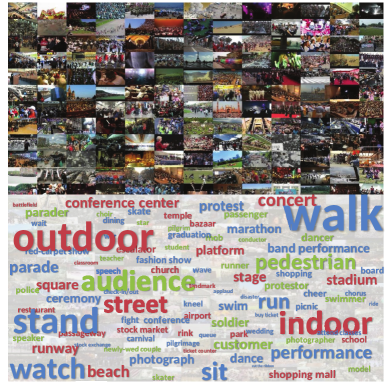
(a) Thumbnails of WWW crowd video dataset and attributesShao2015

(b) Frequencies of attributes

Figure 1: A thumbnail visualisation and a summary on the popularities of all 94 attributes in the WWW crowd video dataset Shao2015 .

More precisely, in this chapter we develop a zero-shot multi-label attribute contextual prediction model (Fig. 2). We make the assumption that the detection of known attributes helps the recognition of unknown ones. For instance, a putative unknown attribute such as “violence” may be related to known attributes “outdoor”, “fight”, “mob”, and “police” among others. Therefore, high confidence in these attributes would support the existence of “violence”. Specifically, our model first learns a probabilistic $P$-way classifier on $\mathit{P}$ known attributes, e.g. $p(``outdoor"|\mathbf{x})$. Then we estimate the probability of each novel (unseen) attribute conditioned on the confidence of $P$ known attributes, e.g. $p(``violence"|``outdoor")$. Recall that due to “violence” in this example being a novel attribute, this conditional probability cannot be estimated directly by tabulation of annotation statistics. To model this conditional, we consider two contextual learning approaches. The first approach relies on the semantic relatedness between the two attributes. For instance, if “fight” is semantically related to “violence”, then we would assume a high conditional probability $p(``violence"|``fight")$. Crucially, such semantic relations can be learned in the absence of annotated video data. This is achieved by using large text corpora GanLYZH_AAAI_15 and language models Mikolov2013a ; pennington2014glove . However, this text-only based approach has the limitation that linguistic relatedness may not correspond reliably to the visual contextual co-occurence that we wish to exploit. For example, the word “outdoor” has high linguistic semantic relatedness, e.g. measured by a cosine similarity, with “indoor”, whilst they would never co-occur in video annotations. Therefore, our second approach to conditional probability estimation is based on learning to map from pairwise linguistic semantic relatedness to visual co-occurence. Specifically, on the known training attributes, we train a bilinear mapping to map the pair of training word-vectors (e.g. $\mathbf{v}(``fight")$ and $\mathbf{v}(``mob")$) to the training attributes’ co-occurrence. This bilinear mapping can then be used to better predict the conditional probability between known and novel/unseen attributes. This is analogous to the standard ZSL idea of learning a visual-semantic mapping from a set of single attributes and re-using this mapping across different unseen attributes. Here, we focus instead on a set of attribute-pairs to learn co-occurrence mapping, and re-using this pairwise mapping across new attribute pairs.

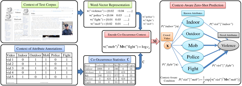
Figure 2: In model training, we learn word-vector representations of training attributes from an external text corpus (context of text corpus), and their visual co-occurrence from the training video annotations (context of attribute annotations). A bilinear mapping $\mathbf{M}$ between pairs of word vectors is trained to predict the log visual co-occurrence statistics $\log c_{ij}$. Visual co-occurrence probabilities can be estimated for any pairs of known or novel (unseen) attributes. To enable the prediction of a novel attribute “violence” using the context of known attributes, we first learn a recogniser for each known attribute given its visual features, e.g. $p(``mob"|x)$; we then use the trained context model to estimate the conditional probability $P(``violence"|``mob")$ between novel and known attributes.

As a proof-of-concept case study, we consider the task of violent behaviour (event) detection in videos. This task has received increasing interest in recent years hassner2012violent , but it is challenging due to the difficulty of obtaining violent event videos for training reliable recognisers. In this chapter, we demonstrate our approach by training our model on an independent large WWW crowd-attribute video dataset, which does not contain “violence” as a known attribute, and then apply the model to violent event detection on the Violent Flow video dataset hassner2012violent .

In summary, we make the following contributions in this chapter: (1) For the first time, we investigate zero-shot learning for crowd behaviour recognition to overcome the costly and semantically ambiguous video annotation of multi-labels. (2) We propose a contextual learning strategy which enhances novel attribute recognition through context prediction by estimating attribute-context co-occurrence with a bilinear model. (3) A proof-of-concept case study is presented to demonstrate the viability of transferring zero-shot recognition of violent event cross-domain with very promising performance.

2 Related Work

2.1 Crowd Analysis

Crowd analysis is one of the central topics in computer vision research for surveillance gong2011security . There are a variety of tasks including: (1) Crowd density estimation and person counting Chen_featuremining ; LoyEtAl_Chapter2013 , (2) crowd tracking ali2008floor ; rodriguez2011data , and (3) crowd behaviour recognition andrade2006modelling ; wang2009unsupervised ; Shao2015 . There are several challenges in crowd behaviour analysis. First of all, one requires both informative and robust visual features from crowd videos. Although simple optical flow Xu:2013:CTS:2510650.2510657 ; rodriguez2011data ; saleemi2010scene , tracklets zhao2012tracking ; zhou2012coherent , or a combination of motion and static features li2012learning have been adopted. None of them is both informative and robust. More desirable Scene-level features can be further constructed from these low-level features, using probabilistic topic models wang2009unsupervised ; Xu:2013:CTS:2510650.2510657 or Gaussian mixtures saleemi2010scene . However, these mid-level representations are mostly scene-specific, with a few exceptions such as Xu:2013:CTS:2510650.2510657 which models multiple scenes to learn a scene-independent representation. Second, for recognition in different scenes, existing methods rely heavily upon the assumption of the availability of sufficient observations (a large number of repetions with variations) from these scenes in order to either learn behaviour models from scratch wang2009unsupervised ; li2012learning ; saleemi2010scene , or inherit models from related scenes Xu:2013:CTS:2510650.2510657 . To generalize models across scenes, studies have proposed scene-invariant crowd/group descriptors inspired by socio-psychological and biological research shao2014scene , and more recently from deep learning mined crowd features Shao2015 . In addition to these purpose-built crowd features, dense trajectory features Wang2014 capturing both dynamic (motion boundary) and static textural information have also been adopted for crowd analysis Shao2015 . For learning a scene-invariant model, the method of Shao2015 requires extensive manual annotation of crowd attributes: The WWW crowd video dataset Shao2015 has 94 attributes captured by over 10,000 annotated crowd videos, where each crowd video is annotated with multiple attributes. The effort required for annotating these videos is huge. This poses significant challenge to scale up the annotation of any larger video dataset from diverse domains. Third, often the most interesting crowd behaviour is also novel in a given scene/domain. That is, the particular behavioural attribute has not been seen previously in that domain. To address these challenges, in this study we explore a different approach to crowd behaviour recognition, by which crowd attribute context is learned from a large body of text descriptions rather than relying on exhaustive visual annotations, and this semantic contextual knowledge is exploited for zero-shot recognition of novel crowd behavioural attributes without labelled training samples.

2.2 Zero-Shot Learning

Zero-shot learning (ZSL) addresses the problem of constructing recognizers for novel categories without labelled training data (unseen) Lampert2009 . ZSL is made possible by leveraging an intermediate semantic space that bridges visual features and class labels (semantics). In general, the class labels can be obtained by manually labelled attributes Lampert2009 ; Fu2015 , word-vector embeddings Socher2013 ; Xu_SES_ICIP15 , structured word databases such as the WordNet Rohrbach2011 ; GanLYZH_AAAI_15 , and co-occurrence statistics from external sources Mensink2014 .

Attributes Attributes are manually defined binary labels of mid-level concepts Lampert2009 which can be used to define high-level classes, and thus bridge known and unknown classes. Traditional supervised classifiers can be trained to predict attributes rather than categories. In the testing phase, recognisers for new classes can then be defined based on novel classes’ attributes, e.g. Direct Attribute Prediction (DAP) Lampert2009 , or relations to known classes by the attributes, e.g. Indirect Attribute Prediciton (IAP) Lampert2009 . This intuitive attribute based strategy inspired extensive research into ZSL. However, attributes themselves are manually annotated and thus suffer from: (i) The difficulty of determining an appropriate ontology of attributes; (ii) Prohibitive annotation cost, in particular for videos due to their spatio-temporal nature; and (iii) labelling each video with a large vocabulary of attributes is particularly costly and ambiguous.

Note that attributes in the context of a ZSL semantic representation are different from the attributes we aim to predict in this chapter. In the attribute-ZSL case, all attributes are pre-defined and annotated in order to train supervised classifiers to generate a representation that bridges known and un-known high-level classes for multi-class ZSL prediction. In our case, we want to predict multiple crowd attributes for each video. That is, our final goal is multi-label ZSL prediction, as some of these attributes are zero-shot, i.e. not pre-defined or annotated in training data.

WordNet As an alternative to attributes, WordNet fellbaum1998wordnet is a large English lexical database which organises words in groups (aka synsets). WordNet is notably exploited for the graph structure which provides a direct relatedness measurement between classes as a path length between concepts Rohrbach2010 ; GanLYZH_AAAI_15 . The IAP model can be implemented without attribute annotation by replacing the novel to known class relation by WordNet induced relation. However, due to the absence of explicit representation for each individual word, the WordNet semantics are less likely to generalize to ZSL models with alternative training losses (e.g. ranking loss and regression loss) which require explicit embedding of words.

Co-occurrence Studies have also explored external sources for measuring the relation between known and novel classes. In particular, web hit count has been considered as a source to induce a co-occurrence based representation Rohrbach2010 ; Mensink2014 . Intuitively, two labels/concepts are treated closely related if they often co-occur in search engine results. As with the WordNet based approaches, co-occurrence models are not able to produce explicit representations for classes therefore are not compatible with learning alternative losses.

Word-Vector The word-vector representation Mikolov2013a ; Socher2013 generated by unsupervised learning on text corpora has emerged as a promising representation for ZSL in that: (i) As the product of unsupervised learning on existing text corpora, it avoids manual annotation bottlenecks; (ii) Semantic similarity between words/phrases can be measured as cosine distance in the word-vector space thus enables probabilistic views of zero-shot learning, e.g. DAPLampert2009 and semantic inter-relations GanLYZH_AAAI_15 , and training with alternative models, e.g. ranking loss akata2015outputEmbedding ; frome2013devise and regression loss Socher2013 ; Xu_SES_ICIP15 .

2.3 Multi-Label Learning

Due to the multiple aspects of crowd behaviour to be detected/recognised, videos are often annotated with more than one attribute. The multi-attribute nature of crowd video, makes crowd behaviour understanding a multi-label learning (MLL) zhang2014review problem. MLL zhang2014review is the task of assigning a single instance simultaneously to multiple categories. MLL can be decomposed into a set of independent single-label problems to avoid the complication of label correlation zhang2007ml ; boutell2004learning . Although this is computationally efficient, ignoring label correlation produces sub-optimal recognition. Directly tackling the joint multi-label problem through considering all possible label combinations is intractable, as the size of the output space and the required training data grow exponentially w.r.t. the number of unique labels tsoumakas2007random . As a compromise, tractable solutions to correlated multi-label prediction typically involve considering pairwise label correlations furnkranz2008multilabel ; qi2007correlative ; ueda2002parametric , e.g. using conditional random fields (CRF)s. However, all existing methods require to learn these pairwise label correlations in advance from the statistics of large labeled datasets. In this chapter, we solve the challenge of multi-label prediction for labels without any existing annotated datasets from which to extract co-occurrence statistics.

2.4 Multi-Label Zero-Shot Learning

Although zero-shot learning is now quite a well studied topic, only a few studies have considered multi-label zero-shot learning Fu2014 ; Mensink2014 . Joint multi-label prediction is challenging because conventional multi-label models require pre-computing the label co-occurrence statistics, which is not available in the ZSL setting. The study given by Fu2014 proposed a Direct Multi-label zero-shot Prediction (DMP) model. This method synthesises a power-set of potential testing label vectors so that visual features projected into this space can be matched against every possible combination of testing labels with simple NN matching. This is analogous to directly considering the jointly multi-label problem, which is intractable due to the size of the label power-set growing exponentially ($2^{n}$) with the number of labels being considered. An alternative study was provided by Mensink2014 . Although applicable to the multi-label setting, this method used co-occurrence statistics as the semantic bridge between visual features and class names, rather than jointly predicting multiple-labels that can disambiguate each other. A related problem is to jointly predict multiple attributes when attributes are used as the semantic embedding for ZSL hariharan2012efficient . In this case, the correlations of mid-level attributes, which are multi-labelled, are exploited in order to improve single-label ZSL, rather than the inter-class correlation being exploited to improve multi-label ZSL.

3 Methodology

We introduce in this section a method for recognising novel crowd behavioural attributes by exploring the context from other recognisable (known) attributes. In section 3.1, we introduce a general procedure for predicting novel behavioural attributes based on their relation to known attributes. This is formulated as a probabilistic graphic model adapted from Lampert2009 and gan2015devnet . We then give the details in section 3.2 on how to learn a behaviour predictor that estimates the relations between known and novel attributes by inferring from text corpus and co-occurrence statistics of known attribute annotations.

Let us first give an overview of the notations used in this chapter in Table 1. Formally we have training dataset $\mathcal{T}^{S}=\{\mathbf{X}^{S},\mathbf{Y}^{S},\mathbf{V}^{S}\}$ associated with $P$ known attributes and testing dataset $\mathcal{T}^{T}=\{\mathbf{X}^{T},\mathbf{Y}^{T},\mathbf{V}^{T}\}$ associated with $Q$ novel/unseen attributes. We denote the visual feature for training and testing videos as $\mathbf{X}^{S}=[\mathbf{x}_{1},\cdots\mathbf{x}_{\mathit{N_{S}}}]\in\mathbb{R}^{\mathit{D}_{x}\times\mathit{N_{S}}}$ and $\mathbf{X}^{T}=[\mathbf{x}_{1},\cdots\mathbf{x}_{\mathit{N_{T}}}]\in\mathbb{R}^{\mathit{D}_{x}\times\mathit{N_{T}}}$, multiple binary labels for training and testing videos as $\mathbf{Y}^{S}=[\mathbf{\tilde{y}}_{1},\cdots\mathbf{\tilde{y}}_{\mathit{N_{S}}}]\in\{0,1\}^{\mathit{P}\times\mathit{N_{S}}}$ and $\mathbf{Y}^{T}=[\mathbf{y^{*}}_{1},\cdots\mathbf{y^{*}}_{\mathit{N_{T}}}]\in\{0,1\}^{\mathit{Q}\times\mathit{N_{T}}}$, and the continuous semantic embedding (word-vector) for training and testing attributes as $\mathbf{V}^{S}=[\mathbf{v}_{1}\cdots\mathbf{v}_{\mathit{P}}]\in\mathbb{R}^{\mathit{D_{v}}\times\mathit{P}}$ and $\mathbf{V}^{T}=[\mathbf{v}_{1}\cdots\mathbf{v}_{\mathit{Q}}]\in\mathbb{R}^{\mathit{D_{v}}\times\mathit{Q}}$. Note that according to the zero-shot assumption, the training and testing attributes are disjoint i.e. $\forall p\in\{1\cdots P\},q\in\{1\cdots Q\}:\mathbf{v}_{p}\in\mathbf{V}^{S},\mathbf{v}_{q}\in\mathbf{V}^{T},\mathbf{v}_{p}\neq\mathbf{v}_{q}$.

Table 1: Notation Summary

black Notation Description $N_{S};~{}N_{T}$ Number of training/source instances ; testing/target instances $D_{x};~{}D_{v}$ Dimension of visual feature; of word-vector embedding $P;~{}Q$ Number of training/source attributes ; testing/target attributes $\mathbf{X}\in\mathbb{R}^{D_{x}\times N}$;  $\mathbf{x}$ Visual feature matrix for N instances; column representing one instance $\mathbf{Y}\in\{0,1\}^{P\times N}$;  $\mathbf{y}$ Binary labels for $N$ instances with $P$ (or $Q$) labels; column representing one instance $\mathbf{V}\in\mathbb{R}^{D_{v}\times P}$;  $\mathbf{v}$ Word-Vector embedding for $P$ (or $Q$) attributes; column representing embedding for one attribute

3.1 Probabilistic Zero-Shot Prediction

To predict novel attributes by reasoning about the relations between known and novel attributes, we formulate this reasoning process as a probabilistic graph (see Fig. 3).

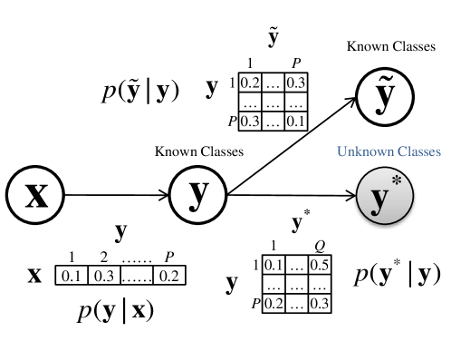
Figure 3: A probablistic graphical representation of a context-aware multi-label zero-shot prediction model.

Given any testing video $\mathbf{x}$, we wish to assign it with one or many of the $\mathit{P}$ known attributes or $\mathit{Q}$ novel attributes. This problem is equivalent to inferring a set of conditional probabilities $p(\mathbf{y^{*}}|\mathbf{x})=\{p({y}^{*}_{q}|\mathbf{x})\}_{q=1\cdots\mathit{Q}}$ and/or $p(\mathbf{\tilde{y}}|\mathbf{x})=\{p(\tilde{y}_{p}|\mathbf{x})\}_{p=1\cdots\mathit{P}}$. To achieve this, given the video instance $\mathbf{x}$, we first infer the likelihood of it being one of the $\mathit{P}$ known attributes as $p(\mathbf{y}|\mathbf{x})=\{p(y_{p}|\mathbf{x})\}_{p=1\cdots P}$. Then, given the relation between known and novel/known attributes as conditional probability $P(\mathbf{y}^{*}|\mathbf{y})$ or $P(\mathbf{\tilde{y}}|\mathbf{y})$, we formulate the conditional probability similar to Indirect Attribute Prediction (IAP) Lampert2009 ; GanLYZH_AAAI_15 as follows:

$$\begin{split}p({y}^{*}_{q}|\mathbf{x})=\sum\limits_{p=1}^{\mathit{P}}p({y}^{*}_{q}|y_{p})p(y_{p}|\mathbf{x})\\ p(\tilde{y}_{\tilde{p}}|\mathbf{x})=\sum\limits_{p=1}^{\mathit{P}}p(\tilde{y}_{\tilde{p}}|y_{p})p(y_{p}|\mathbf{x})\end{split}$$ (1)

The zero-shot learning task is to infer the probabilities $\{p({y}^{*}_{q}|\mathbf{x})\}_{p=1\cdots\mathit{P}}$ for unseen labels $\{y^{*}_{q}\}$. We estimate the multinomial conditional probability of known attributes $p(y_{p}|\mathbf{x})$ based on the output of a probabilistic P-way classifier, e.g. SVM or Softmax Regression with probability output. Then the key to the success of zero-shot prediction is to estimate the known to novel contextual attribute relation as conditional probabilities $\{p({y}^{*}_{q}|y_{p})\}$. We introduce two approaches to estimate this contextual relation.

3.2 Modelling Attribute Relation from Context

In essence, our approach to the prediction of novel attributes depends on the prediction of known attributes and then predicting the novel attributes based on the confidence of each known attribute. The key to the success of this zero-shot prediction is therefore appropriately estimating the conditional probability of novel attribute given known attributes. We first consider a more straightforward way to model this conditional by exploiting the relation encoded by a text corpus GanLYZH_AAAI_15 . We then extend this idea to predict the expected visual co-occurrence between novel and known attributes without labelled samples of the novel classes.

Learning Attribute Relatedness from Text Corpora

The first approach builds on semantic word embedding GanLYZH_AAAI_15 . The semantic embedding represents each English word as a continuous vector $\mathbf{v}$ by training a skip-gram neural network on a large text corpus Mikolov2013a . The objective of this neural network is to predict the blackadjacent $c$ words to the current word $w_{t}$, as follows:

$$\frac{1}{\mathit{T}}\sum\limits_{t=1}^{\mathit{T}}\sum\limits_{-c\leq j\leq c,j\neq 0}p(w_{t+j}|w_{t})$$ (2)

The conditional probability is modelled by a softmax function, a normalised probability distribution, based on each word’s representation as a continuous vector:

$$p(w_{t+j}|w_{t})=\frac{exp(\mathbf{v}_{t+j}^{\top}\mathbf{v}_{t})}{\sum\limits_{j=1}^{W}exp(\mathbf{v}_{t+j}^{\top}\mathbf{v}_{t})}$$ (3)

By maximizing the above objective function, the learned word-vectors $\mathbf{V}=\{\mathbf{v}\}$ capture contextual co-occurrence in the text corpora so that frequently co-occurring words result in high cumulative log probability in Eq (2). We apply the softmax function to model conditional attribute probability black as Eq (4) where $\gamma$ is a temperature parameter.

$$p({y}^{*}_{q}|y_{p})=\frac{exp(\frac{1}{\gamma}\mathbf{v}_{q}^{\top}\mathbf{v}_{p}^{S})}{\sum\limits_{p=1}^{P}exp(\frac{1}{\gamma}\mathbf{v}_{q}^{\top}\mathbf{v}^{S}_{p})}$$ (4)

This can be understood intuitively from the following example: An attribute “Shopping” has high affinity with attribute “ShoppingMall” in word-vector inner product because they co-occur in the text corpus. Our assumption is that the existence of known video attribute “Shopping” would support the prediction of unseen attribute “ShoppingMall”.

Context Learning from Visual Co-Occurrence

Although attribute relations can be discovered from text context as described above, these relations may not ideally suit crowd attribute prediction in videos. For example, the inner product of $vec(``Indoor")$ and $vec(``Outdoor")$ is $0.7104$ which is ranked the 1st w.r.t. “Indoor” among 93 attributes in the WWW crowd video dataset. As a result, the estimated conditional probability $p(\tilde{y}_{Indoor}|y_{Outdoor})$ is the highest among all $\{p(\tilde{y}_{Indoor}|y_{p})\}_{p=1\cdots\mathit{P}}$. However, whilst these two attributes are similar because they occur nearby in the text semantical context, it is counter-intuitive for visual co-occurrence as a video is very unlikely to be both indoor and outdoor. Therefore in visual context, their conditional probability should be small rather than large.

To address this problem, instead of directly paramaterising the conditional probability using word-vectors, we use pairs of word vectors to predict the actual visual co-occurrence. More precisely, we train a word-vector$\to$co-occurrence predictor based on an auxiliary set of known attributes annotated on videos, for which both word-vectors and annotations are known. We then re-deploy this learned predictor for zero-shot recognition on novel attributes. Formally, given binary multi-label annotations $\mathbf{Y}^{S}$ on training video data, we define the contextual attribute occurrence as $\mathbf{C}={\mathbf{Y}^{S}}{\mathbf{Y}}^{S\top}$. The occurrence of $j$-th attribute in the context of $i$-th attribute is thus $\mathit{c}_{ij}$ of the $\mathbf{C}$. The prevalence of $i$-th attribute is defined as $\mathit{c}_{i}=\sum_{j}\mathit{c}_{ij}$. The normalized co-occurrence thus defines the conditional probability as:

$$p(\tilde{y}_{j}|\tilde{y}_{i})=\frac{c_{ij}}{c_{i}}$$ (5)

The conditional probability can only be estimated based on visual co-occurrence in the case of training attributes with annotations $\mathbf{Y}^{S}$. To estimate the conditional probability for testing data of novel attributes without annotations $\mathbf{Y}^{T}$, we consider to predict the expected co-occurrence based on a bilinear mapping $\mathbf{M}$ from the pair of word-vectors. Specifically, we approximate the un-normalized co-occurrence as $exp(\mathbf{v}_{i}^{\top}\mathbf{M}\mathbf{v}_{j})=\mathit{c}_{ij}$. To estimate $\mathbf{M}$, we optimise the regularised linear regression problem:

$$J=\sum\limits_{i}^{P}\sum\limits_{j}^{P}w(\mathit{c}_{ij})\left(\mathbf{v}_{i}^{\top}\mathbf{M}\mathbf{v}_{j}-\log\mathit{c}_{ij}\right)^{2}+\lambda||\mathbf{M}||_{F}^{2},$$ (6)

blackwhere $\lambda$ is the regularisation strength, and a weight function $w(c_{ij})$ is applied to the regression loss function above in order to penalise rarely occurring co-occurrence statistics. We choose the weight function according to Mensink2014 , which is:

$$w(c_{ij})=\left(\frac{c_{ij}}{\mathit{C_{max}}}\right)^{(\alpha\cdot\text{1}(c_{ij}\leq\mathit{C}_{max}))}$$ (7)

where $\mathit{C}_{max}$ is a threshold of co-occurrence, black$\alpha$ controls the increasing rate of the weight function and the 1 is an indicator function. This bilinear mapping is related to the model in pennington2014glove , but differs in that: (i) The input of the mapping is the word-vector representations $\mathbf{v}$ learned from the skip-gram model Mikolov2013a in order to generalise to novel attributes where no co-occurrence statistics are available. (ii) The mapping is trained to account for visual compatibility, e.g. “Outdoor” is unlikely to co-occur with “Indoor” in a visual context, although the terms are closely related in their representations learned from the text corpora alone. The bilinear mapping can be seamlessly integrated with the softmax conditional probability as:

$$p(y^{*}_{q}|y_{p})=\frac{exp(\mathbf{v}_{q}^{\top}\mathbf{M}\mathbf{v}_{p})}{\sum\limits_{p}exp(\mathbf{v}_{q}^{\top}\mathbf{M}\mathbf{v}_{p})}$$ (8)

Note that by setting $\mathbf{M}=\mathbf{I}$, this conditional probability degenerates to the conventional word-vector based estimation in Eq (4). The regression to predict visual co-occurrence from word-vectors (Eq. (6)) can be efficiently solved by gradient descent using the following gradient:

$$\nabla\mathbf{M}=\sum\limits_{i=1}^{\mathit{P}}\sum\limits_{j=1}^{\mathit{P}}f(\mathit{c}_{ij})\left(2\mathbf{v}_{i}\mathbf{v}_{i}^{\top}\mathbf{M}\mathbf{v}_{j}\mathbf{v}_{j}^{\top}-2\log\mathit{c}_{ij}\mathbf{v}_{i}\mathbf{v}_{j}^{\top}\right)+2\lambda\mathbf{M}$$ (9)

4 Experiments

We evaluate our multi-label crowd behaviour recognition model on the large WWW crowd video dataset Shao2015 . We analyse each component’s contribution to the overall multi-label ZSL performance. Moreover, we present a proof-of-concept case study for performing transfer zero-shot recognition of violent behaviour in the Violence Flow video dataset hassner2012violent .

4.1 Zero-Shot Multi-Label Behaviour Inference

Experimental Settings

Dataset

The WWW crowd video dataset is specifically proposed for studying scene-independent attribute prediction for crowd scene analysis. It consists of over 10,000 videos collected from online resources of 8,257 unique scenes. The crowd attributes are designed to answer the following questions: “Where is the crowd”, “Who is in the crowd” and “Why is the crowd here”. All videos are manually annotated with 94 attributes with 6 positive attributes per video on average. Fig.4 shows a collection of 94 examples with each example illustrating each attribute in the WWW crowd video dataset.

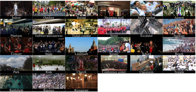
(a) 27 attributes by “Where”

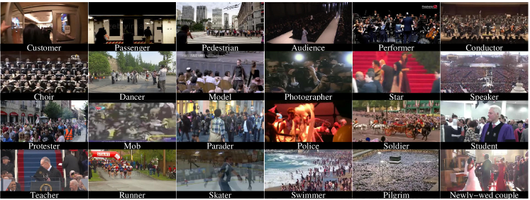
(b) 24 attributes by “Who”

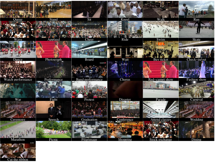
(c) 44 attributes by “Why”

Figure 4: Examples of all attributes in the WWW crowd video dataset Shao2015 .

Data Split

We validated the ability to utilise known attributes for recognising novel attributes in the absence of training samples on the WWW dataset. To that end, we divided the 94 attributes into 85 for training (known) and 9 for testing (novel). This was repeated for 50 random splits. In every split, any video which has no positive label from the 9 novel attributes was used for training and the rest for testing. The distributions of the number of multi-attributes (labels) per video over all videos and over the testing videos are shown in Fig 5(a-b) respectively. Fig 5(c) also shows the distribution of the number of testing videos over the 50 random splits. In most splits, the number of testing videos is in the range of 3,000 to 6,000. The training to testing video number ratio is between 2:1 to 1:1. This low training-testing ratio makes for a challenging zero-shot prediction setting.

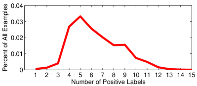
(a) Label distribution over all videos

(b) Label distribution over testing videos

(c) Distribution of testing videos

Figure 5: Statistics of the dataset split for our experiments on the WWW dataset. (a) and (b): The distributions of multi-label per video over all the videos and over the testing videos respectively. (c): The distribution of the number of testing videos over all 50 random splits.

Visual Features

Motion information can play an important role in crowd scene analysis. To capture crowd dynamics, we extracted the improved dense trajectory features Wang2014 and performed Fisher vector encoding Perronnin2010 on these features, generating a $50,688$ dimensional feature vector to represent each video.

Evaluation Metrics

We evaluated the performance of multi-label prediction using five different metrics zhang2014review . These multi-label prediction metrics fall into two groups: Example-based metric and label-based metric. Example-based metrics evaluate the performance per video instance and then average over all instances to give the final metric. Label-based metrics evaluate the performance per label category and return the average over all label categories as the final metric. The five multi-label prediction performance metrics are:

• AUC - The Area Under the ROC Curve. AUC evaluates binary classification performance. It is invariant to the positive/negative ratio of each testing label. Random guess leads to AUC of 0.5. For multi-label prediction, we measure the AUC for each testing label and average the AUC over all 50 splits to yield the AUC per category. The final mean AUC is reported as the mean over all lable categories.

• Label-based AP - Label-based Average Precision. We measure the average precision for each attribute as the average fraction of relevant videos ranked higher than a threshold. The random guess baseline for label-based AP is determined by the prevalence of positive videos.

• Example-based AP - Example-based Average Precision. We measure the average precision for each video as the average fraction of relevant label prediction ranked higher than a threshold. Example-based AP focuses on the rank of attributes within each instance rather than rank of examples for each label as for label-based AP.

• Hamming Loss - Hamming Loss measures the percentage of incorrect predictions from groundtruth labels. Optimal hamming loss is 0, indicating perfect prediction. Due to the nature of hamming loss, the distance of $[000]$ and $[110]$ w.r.t. $[010]$ are equal. Thus it does not differentiate over-estimation from under-estimation. Hamming loss is a label-based metric. The final mean is reported as the average over all instances.

• Ranking Loss - Ranking Loss measures, for every instance, the percentage of negative labels ranked higher than positive labels among all possible positive-negative label pairs. Similar to example-based AP, the ranking loss is example-based metric focusing on pushing positive labels ahead of negative labels for each instance.

Both AUC and label-based AP are label-based metrics, whilst exampled-based AP, Hamming Loss and Ranking Loss are example-based metrics. Moreover, as a loss metric, both Hamming Loss and Ranking Loss values are lower the better. In contrary, AUC and AP values are higher the better. In a typical surveillance application of crowd behaviour recognition in videos, we are interested in detecting video instances of a particular attribute that triggers an alarm event, e.g. searching for video instances with the “fighting” attribute. In this context, label-based performance metrics such as AUC and Label-based AP are more relevant. Overall, we present model performance evaluated by both types of evaluation metrics.

black

Parameter Selection

We have several parameters to tune in our model. Specifically, for training SVM classifiers for known classes/attributes $\{p(y|\mathbf{x})\}$ we set the slack parameter to a constant 1. The ridge regression coefficient $\lambda$ in Eq (6) is essential to avoid over-fitting and numerical problems. It is empirically set to small non-zero value. We choose $\lambda=1^{-3}$ in our experiments. For the temperature parameter $\gamma$ in Eq (4), we cross validate and found best value to be around $0.1$. In addition, we use a word-vector dictionary pre-trained on Google News dataset Mikolov2013a with 100 billion words where word-vectors are trained with 300 dimension ($D_{v}=300$) and context size 5 ($c=5$).

Comparative Evaluation

In this first experiment, we evaluated zero-shot multi-label prediction on WWW crowd video dataset. We compared our context-aware multi-label ZSL models, both purely text-based and visual co-occurrence based, against four contemporary and state-of-the-art zero-shot learning models.

Sate-of-the-art ZSL Models

1. Word-Vector Embedding (WVE) Xu_SES_ICIP15 : The WVE model constructs a vector representation $\mathbf{z}_{tr}=g(\mathit{y}_{tr})$ for each training instance according to its category name $\mathit{y}_{tr}$ via word-vector embedding $g(\cdot)$ and then learns a support vector regression $f(\cdot)$ to map the visual feature $\mathbf{x}_{tr}$. For testing instance $\mathbf{x}_{te}$, it is first mapped into the semantic embedding space via the regressor $f(\mathbf{x}_{te})$. Novel category $\mathit{y}_{te}\in\mathcal{Y}_{te}=\{1,\cdots Q\}$ is then mapped into the embedding space via $g(\mathit{y}_{te})$. Nearest neighbour matching is applied to match $\vec{x}_{te}$ with category $\mathit{y}^{*}$ using the L2 distance:

   $$\mathit{y}^{*}=\arg\min\limits_{y_{te}\in\mathcal{Y}_{te}}||f(\mathbf{x}_{te})-g(\mathit{y}_{te})||_{2}^{2}$$ (10)

   We do not assume having access to the whole testing data distribution, so we do not exploit transductive self-training and data augmentation post processing, unlike in the cases of Xu_SES_ICIP15 ; AlexiouXG_ICIP16 .

2. Embarrassingly Simple Zero-Shot Learning (ESZSL) romera2015embarrassingly : The ESZSL model considers ZSL as training a L2 loss classifier. Specifically, given known categories’ binary labels $\mathbf{Y}$ and word-vector embedding $\mathbf{V}_{tr}$, we minimise the L2 classification loss as:

   $$\min\limits_{\mathbf{M}}\sum\limits_{i=1}^{\mathit{N}}||\mathbf{x}_{i}^{\top}\mathbf{M}\mathbf{V}_{tr}-\mathbf{y}_{i}||^{2}_{2}+\Omega(\mathbf{M};\mathbf{V}_{tr},\mathbf{X})$$ (11)

   blackwhere $\Omega(\mathbf{M};\mathbf{V}_{tr},\mathbf{X})$ is a regulariser defined as:

   black

   $$\Omega(\mathbf{M};\mathbf{V}_{tr},\mathbf{X})=\lambda_{1}||\mathbf{M}\mathbf{V}_{tr}||_{F}^{2}+\lambda_{2}||\mathbf{X}^{\top}\mathbf{M}||_{F}^{2}+\lambda_{3}||\mathbf{M}||_{F}^{2}$$ (12)

   Novel categories are predicted by:

   $$\mathbf{y}^{*}=\mathbf{x}_{te}^{\top}\mathbf{M}\mathbf{V}_{te}$$ (13)

3. Extended DAP (ExDAP) Fu2014 : ExDAP was specifically proposed for multi-label zero-shot learning Fu2014 . This is an extension of single-label regression models to multi-label. Specifically, given training instances $\mathbf{x}_{i}$, associated multiple binary labels $\mathbf{y}_{i}$, and word-vector embedding of known labels $\mathbf{V}_{tr}$, we minimize the L2 regression loss for learning a regressor $\mathbf{M}$:

   $$\min\limits_{\mathbf{M}}\sum\limits_{i=1}^{\mathit{N}}||\mathbf{x}_{i}^{\top}\mathbf{M}-\mathbf{V}_{tr}\mathbf{y}_{i}||_{2}^{2}+\lambda||\mathbf{M}||_{2}^{2}$$ (14)

   For zero-shot prediction, we minimize the same loss but w.r.t. the binary label vector $\mathbf{y}$ with L2 regularization:

   $$\mathbf{y}^{*}=\arg\min\limits_{\mathbf{y^{*}\in\mathbb{R}}}||\mathbf{x}_{te}^{\top}\mathbf{M}-\mathbf{V}_{te}\mathbf{y^{*}}||_{2}^{2}+\lambda||\mathbf{y}^{*}||_{2}^{2}$$ (15)

   A closed-form solution exists for prediction:

   $$\mathbf{y}^{*}=\left(\mathbf{V}_{te}^{\top}\mathbf{V}_{te}+\lambda\mathbf{I}\right)^{-1}\mathbf{V}_{te}^{\top}\mathbf{x}_{te}^{\top}\mathbf{M}$$ (16)

4. Direct Multi-Label Prediction (DMP) Fu2014 : DMP was proposed to exploit the correlation between testing labels so to benefit the multi-label prediction. It shares the same training procedure with ExDAP in Eq (14). For zero-shot prediction, given testing categories $\mathcal{Y}_{te}$ we first synthesize a power-set of all labels $\mathcal{P}(\mathcal{Y}_{te})$. The multi-label prediction $\mathbf{y}^{*}$ is then determined by nearest neighbour matching of visual instances mapped into word-vector embedding $\mathbf{x}_{te}^{\top}\mathbf{M}$ against the synthesized power-set:

   $$\mathbf{y}^{*}=\arg\min\limits_{\mathbf{y}^{*}\in\mathcal{P}(\mathcal{Y}_{te})}||\mathbf{x}_{te}^{\top}\mathbf{M}-\mathbf{V}_{te}\mathbf{y}^{*}||_{2}^{2}$$ (17)

Context-Aware Multi-Label ZSL Models

1. Text Context-Aware ZSL (TexCAZSL): In our text corpus context-aware model introduced in Section 3.2, only word-vectors learned from text corpora Mikolov2013a are used to model the relation between known and novel attributes $p(\mathbf{y}^{*}|\mathbf{y})$, as defined by Eq (4). We implemented the video instance to known attributes probabilities $p({y}_{p}|\mathbf{x})$ as $\mathit{P}$ linear SVM classifiers with normalized probability outputs CC01a . Novel attribute prediction $p({y}^{*}_{q}|\mathbf{x})$ is computed by marginalising over the known attributes defined by Eq (1).

2. Visual Co-occurrence Context-Aware ZSL (CoCAZSL): We further implemented a visual co-occurrence context-aware model built on top of the TexCAZSL model. This is done by predicting the expected co-occurrence context using bilinear mapping $\mathbf{M}$, as introduced in Section 3.2. The known to novel attribute relation is thus modelled by a weighted inner-product between the word-vectors of known and novel attributes given by Eq (8). Novel attribute prediction $p({y}^{*}_{q}|\mathbf{x})$ is computed in the same way as for TexCAZSL, defined by Eq (1).

Quantitative Comparison

Table 2 shows the comparative results of our models against four state-of-the-art ZSL models and the baseline of “Random Guess”, using all five evaluation metrics. Three observations can be made from these results: (1) All zero-shot learning models can substantially outperform random guessing, suggesting that zero-shot crowd attribute prediction is valid. This should inspire more research into zero-shot crowd behaviour analysis in the future. (2) It is evident that our context-aware models improve on existing ZSL methods when measured by the label-based AUC and AP metrics. As discussed early under evaluation metrics, for typical surveillance tasks, label-based metrics provide a good measurement on detecting novel alarm events in the mist of many other contextual attributes in crowd scenes. (3) It is also evident that our context-aware models perform comparably to the alternative ZSL models under the example-based evaluation metrics, with the exception that DMP Fu2014 performs extraordinarily well on Hamming Loss but poorly on Ranking Loss. This is due to the direct minimization of Hamming Loss between synthesized power-set and embedded video in DMP. However, since the relative order between attributes are ignored in DMP, low performance in ranking loss as well as other label-based metrics is expected.

Table 2: Comparison of zero-shot multi-label attribute prediction on the WWW crowd video dataset. The $\uparrow$ and $\downarrow$ symbols indicate whether a metric is higher the better or vice versa.

Feature	Model	Label-Based		Example-Based
		AUC $\uparrow$	AP $\uparrow$	AP $\uparrow$	Hamming Loss $\downarrow$	Ranking Loss $\downarrow$
-	Random Guess	0.50	0.14	0.31	0.50	-
ITF	WVEXu_SES_ICIP15	0.65	0.24	0.52	0.45	0.32
ITF	ESZSLromera2015embarrassingly	0.63	0.22	0.53	0.46	0.32
ITF	ExDAPFu2014	0.62	0.21	0.52	0.45	0.32
ITF	DMPFu2014	0.59	0.20	0.45	0.30	0.70
ITF	TexCAZSL	0.65	0.24	0.52	0.43	0.32
ITF	CoCAZSL	0.69	0.27	0.53	0.42	0.31

Qualitative Analysis

We next give some qualitative examples of zero-shot attribute predictions in Fig. 6. To get a sense of how well the attributes are detected in the context of label-based AP, we present the AP number with each attribute. Firstly, we give examples of detecting videos matching some randomly chosen attributes (label-centric evaluation). By designating an attribute to detect, we list the crowd videos sorted in the descending order of probability $p(y^{*}|\mathbf{x})$. In general, we observe good performance in ranking crowd videos according to the attribute to be detected. The false detections are attributed to the extremely ambiguous visual cues. E.g. 3rd video in “fight”, 5th video in “police” and 2nd video in “parade” are very hard to interpret.

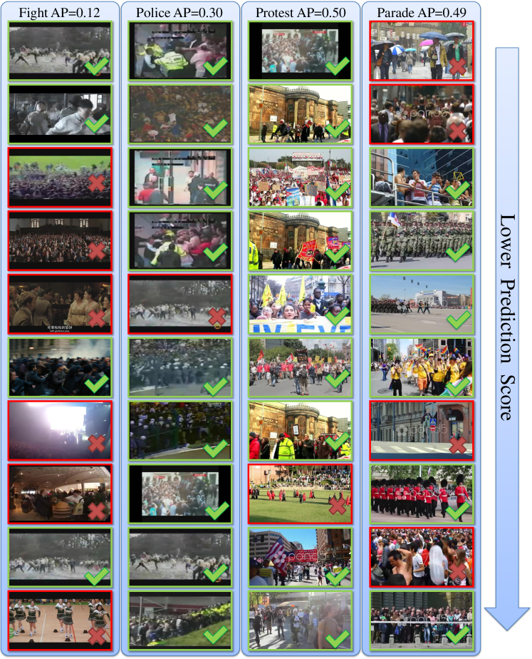
Figure 6: Illustration of crowd videos ranked in accordance with prediction scores (marginalized conditional probability) w.r.t. each attribute.

In addition to detecting each individual attribute, we also present some examples of simultaneously predicting multiple attributes in Fig.7 (example-centric evaluation). For each video we give the the prediction score for all testing attributes as $\{p(y^{*}_{q}|\mathbf{x})\}_{q=1\cdots\mathit{Q}}$ . For the ease of visualization, we omit the the attribute with least score. We present the example-based ranking loss number along with each video to give a sense of how the quantitative evaluation metric relates to the qualitative results. In general, ranking loss less than $0.1$ would yield very good multi-label prediction as all labels would be placed among the top 3 out of 9 labels to be predicted. Whilst ranking loss around $0.3$ (roughly the average performance of our CoCAZSL model, see Table 2) would still give reasonable predictions by placing positive labels in the top 5 out of 9.

Figure 7: Examples of zero-shot multi-label attribute prediction. Bars under each image indicate the normalized score for testing attribtues. Blue and pink bars indicate positive and negative ground-truth labels respectively.

4.2 Transfer Zero-Shot Recognition in Violence Detection

Recognizing violence in surveillance scenario has an important role in safety and security hassner2012violent ; gong2011security . However due to the sparse nature of violent events in day to day surveillance scenes, it is desirable to exploit zero-shot recognition to detect violent events without human annotated training videos. Therefore we explore a proof of concept case study of transfer zero-shot violence detection. We learn to recognize labelled attributes in WWW dataset Shao2015 and then transfer the model to detect violence event in Violence Flow dataset hassner2012violent . This is zero-shot because we use no annotated examples of violence to train, and violence does not occur in the label set of WWW. It is contextual because the violence recognition is based on the predicted visual co-occurrence between each known attribute in WWW and the novel violence attribute. E.g., “mob” and “police” attributes known from WWW may support the violence attribute in the new dataset.

Experiment Settings

Dataset

The Violence Flow dataset hassner2012violent was proposed to facilitate the study into classifying violent events in crowded scenes. 246 videos in total are collected from online video repositories (e.g. YouTube) with 3.6 seconds length on average. Half of the 246 video are with positive violence content and the another half are with non-violent crowd contents. We illustrate example frames of both violent and non-violent videos in Fig. 8

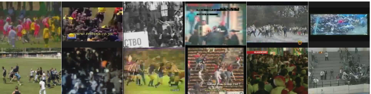
(a) Violent videos

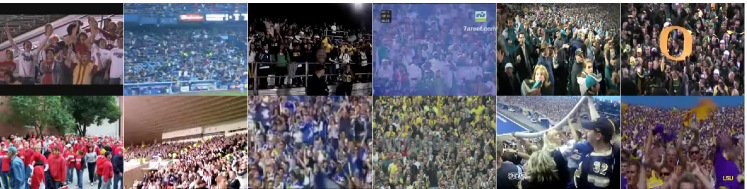
(b) Non-violent videos

Figure 8: Example frames of violence flow dataset hassner2012violent .

Data Split

A standard fully supervised 5-fold cross validation split was proposed by hassner2012violent . The standard split partitions the whole dataset into 5 splits each of which is evenly divided into positive and negative videos. For each testing split, the other 4 splits are used as the training set and the left-out one is the testing set. Results are reported as both the mean classification accuracy over 5 splits plus standard deviation and the area under the ROC curve (AUC).

Beyond the standard cross validation split we create a new zero-shot experimental design. Our zero-shot split learns attribute detection models on all 94 attributes from WWW dataset and then tests on the same testing set as the standard 5 splits in hassner2012violent . We note that there are 123 overlapped videos between WWW and Violence Flow. To make fair comparison, we exclude these overlapped videos from constructing the training data for 94 attributes. In this way zero-shot prediction performance can be directly compared with supervised prediction performance using AUC metric. We define the event/attribute to be detected as the word “violence”.

Zero-Shot Recognition Models

We explore the transfer zero-shot violence recognition by comparing the same set of zero-shot learning models as in Section 4.1: competitors WVE, ESZSL, ExDAP; and our TexCAZSL and CoCAZSL.

Fully Supervised Model

To put zero-shot recognition performance in context, we also report fully supervised models’ performance. These models are evaluated on the 5-fold cross-validation split and the average accuracy and AUC are reported. Specifically, we report the best performance of hassner2012violent - linear SVM with VIolent Flows (ViF) descriptor and our fully supervised baseline - linear SVM with Improved Trajectory Feature (ITF).

Results and Analysis

The results of both transfer zero-shot and supervised violence prediction are summarised in Table 3. We make the following observations: Our context-aware models perform consistently better than alternative zero-shot models, suggesting that context does facilitate zero-shot recognition. Surprisingly, our zero-shot models moreover perform very competitively compared to the fully supervised models. Our CoCAZSL (albeit with better ITF feature) beats the fully supervised Linear SVM with ViF feature in AUC metric (87.22 v.s. 85.00). The context-aware model is also close to the fully supervised model with the same ITF feature (87.22 v.s. 98.72). This is in contrast to the common result in the literature were zero-shot recognition “works”, but does so much worse than fully supervised learning. The promising performance is partly due to modelling the co-occurrence on large known crowd attributes help the correct prediction of known to novel attribute relation prediction.Overall the result shows that by transferring our attribute recognition model trained for a wide set of 94 attributes on a large 10,000 video dataset, it is possible to perform effective zero-shot recognition of a novel behaviour type in a new dataset.

Table 3: Evaluation of violence prediction in Violence Flow dataset: zero-shot versus fully supervised prediction ($\%$).

Model	Split	Feature	Accuracy	AUC
WVEXu_SES_ICIP15	Zero-Shot	ITF	64.27$\pm$5.06	64.25
ESZSLromera2015embarrassingly	Zero-Shot	ITF	61.30$\pm$8.28	61.76
ExDAPFu2014	Zero-Shot	ITF	54.47$\pm$7.37	52.31
TexCAZSL	Zero-Shot	ITF	67.07$\pm$3.87	69.95
CoCAZSL	Zero-Shot	ITF	80.52$\pm$4.67	87.22
Linear SVM	5-fold CV	ITF	94.72$\pm$4.85	98.72
Linear SVMhariharan2012efficient	5-fold CV	ViF	81.30$\pm$0.21	85.00

5 Further Analysis

In this section we provide further analysis on the importance of the visual feature used, and also give more insight into how our contextual zero-shot multi-label prediction works by visualising the learned label-relations.

5.1 Feature Analysis

We first evaluate different static and motion features on the standard supervised attribute prediction task. Both hand-crafted and deeply learned features are reported for comparison.

Static Features

We report the both the hand-crafted and deeply learned static feature from Shao2015 including Static Feature (SFH) and Deeply Learned Static Feature (DLSF). SFH captures general image content by extracting Dense SIFTLazebnik2006 , GIST Oliva2001 and HOG Dalal2005 . Color histogram in HSV space is further computed to capture global information and LBP Zhao2012 is extracted to quantify local texture. Bag of words encoding is used to create comparable features, leading to a 1536 dimension static feature. DLSF is initialized using a pre-trained model for ImageNet detection task ouyang2014deepid and then fine-tuned on the WWW attribute recognition task with cross-entropy loss.

Motion Features

We report both the hand-crafted and deeply learned motion features from Shao2015 including DenseTrackwang2011action , spatio-temporal motion patterns (STMP) kratz2009anomaly and Deeply Learned Motion Feature (DLMF) Shao2015 . Apart from the reported evaluations, we compare them with the improved trajectory feature (ITF) Wang2014 with fisher vector encoding. Though ITF is constructed in the same way as DenseTrack reported in Shao2015 , we make a difference in that the visual codebook is trained on a collection of human action datasets (HMDB51Kuehne2011 , UCF101 Soomro2012 , Olympic Sports NieblesCL_eccv10 and CCVconf/mir/JiangYCEL11 ).

Analysis

Performance on the standard WWW split Shao2015 for static and motion features is reported in Table 4. We can clearly observe that the improved trajectory feature is consistently better than all alternative static and motion features. Surprisingly, ITF is even able to beat deep features (DLSF and DLMF). We attribute this to ITF’s ability to capture both motion information by motion boundary histogram (MBH) and histogram of flow (HoF) descriptors and texture information by Histogram of Gradient (HoG) descriptor.

More interestingly, we demonstrate that motion feature encoding model (fisher vector) learned from action datasets can benefit the crowd behaviour analysis. Due to the vast availability of action and event datasets and limited crowd behaviour data, a natural extension work is to discover if deep motion model pre-trained on action or event dataset can help crowd analysis.

Table 4: Comparison between different visual features for attribute prediction.

Alternative Features	Mean AUC
SFH Shao2015	0.81
DLSF Shao2015	0.87
DenseTrack Shao2015	0.63
DLMF Shao2015	0.68
SFH+DenseTrack Shao2015	0.82
DLSF+DLMF Shao2015	0.88
Our Features
Improved Trajectory Feature (ITF)	0.91

5.2 Qualitative Illustration of Contextual Co-occurrence Prediction

Recall that the key step in our method’s approach to zero-shot prediction is to estimate the visual co-occurrence (between known attributes and held out zero-shot attributes) based on the textually derived word-vectors of each attributes. To illustrate what is learned, we visualize the predicted importance of 94 attributes from WWW in terms of supporting the detection of the held out attribute “violence”. The results are presented as a word cloud in Fig. 9, where the size of each word/attribute $p$ is proportional to the conditional probability e.g. $p(``violence"|y_{p})$. As we see from Fig 9(a), attribute - “fight” is the most prominent attribute supporting the detection of “violence”. Besides this, actions like “street”, “outdoor” and “wave” all support the existence of “violence”, while ‘disaster’ and ‘dining’ among others do not. We also illustrate the support of “mob” and “marathon” in Fig 9(b) and (c) respectively. All these give us very reasonable importance of known attributes in supporting the recognition of novel attributes.

(a) “violence” as novel event

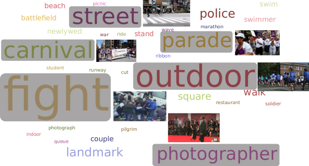
(b) “mob” as novel attribute

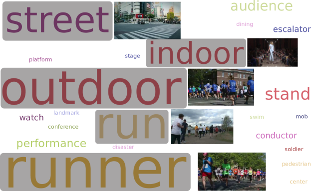
(c) “marathon” as novel attribute

Figure 9: Importantce of known attributes w.r.t. novel event/attributes. The fontsize of each attributes is proportional to the conditional probability e.g. $p(``violence"|y_{p})$.

6 Conclusions

Crowd behaviour analysis has long been a key topic in computer vision research. Supervised approaches have been proposed recently. But these require exhaustively obtaining and annotating examples of each semantic attribute, preventing this strategy from scaling up to ever expanding dataset sizes and variety of attributes. Therefore it is worthwhile to develop recognizers that require little or no annotated training examples for the attribute/event of interest. We address this by proposing a zero-shot learning strategy in which recognizers for novel attributes are built without corresponding training data. This is achieved by learning the recognizers for known labelled attributes. For testing data, the confidence of belonging to known attributes then supports the recognition of novel ones via attribute relation. We propose to model this relation from the co-occurrence context provided by known attributes and word-vector embeddings of the attribute names from text corpora. Experiments on zero-shot multi-label crowd attribute prediction prove the feasibility of zero-shot crowd analysis and demonstrate the effectiveness of learning contextual co-occurrence. A proof of concept case study on transfer zero-shot violence recognition further demonstrates the practical value of our zero-shot learning approach , and its superior efficacy compared to even fully supervised learning approaches.

References

- [1] Zeynep Akata, Scott Reed, Daniel Walter, Honglak Lee, and Bernt Schiele. Evaluation of output embeddings for fine-grained image classification. In CVPR, 2015.
- [2] Ioannis Alexiou, Tao Xiang, and Shaogang Gong. Exploring synonyms as context in zero-shot action recognition. In ICIP, 2016.
- [3] Saad Ali and Mubarak Shah. Floor fields for tracking in high density crowd scenes. In ECCV, 2008.
- [4] Ernesto L Andrade, Scott Blunsden, and Robert B Fisher. Modelling crowd scenes for event detection. In ICPR, 2006.
- [5] Matthew R Boutell, Jiebo Luo, Xipeng Shen, and Christopher M Brown. Learning multi-label scene classification. Pattern recognition, 2004.
- [6] Chih-Chung Chang and Chih-Jen Lin. LIBSVM: A library for support vector machines. ACM Transactions on Intelligent Systems and Technology, 2011. Software available at http://www.csie.ntu.edu.tw/~cjlin/libsvm.
- [7] Ke Chen, Chen Change Loy, Shaogang Gong, and Tao Xiang. Feature mining for localised crowd counting. In BMVC, 2012.
- [8] Navneet Dalal and Bill Triggs. Histograms of oriented gradients for human detection. In CVPR, 2005.
- [9] Christiane Fellbaum. WordNet. Wiley Online Library.
- [10] Andrea Frome, Greg S Corrado, Jon Shlens, Samy Bengio, Jeff Dean, Tomas Mikolov, et al. Devise: A deep visual-semantic embedding model. In NIPS, 2013.
- [11] Yanwei Fu, Timothy M Hospedales, Tao Xiang, and Shaogang Gong. Transductive Multi-view Zero-Shot Learning. IEEE Transactions on Pattern Analysis and Machine Intelligence, 2015.
- [12] Yanwei Fu, Yongxin Yang, Timothy M Hospedales, Tao Xiang, and Shaogang Gong. Transductive Multi-Label Zero-shot Learning. In BMVC, 2014.
- [13] Johannes Fürnkranz, Eyke Hüllermeier, Eneldo Loza Mencía, and Klaus Brinker. Multilabel classification via calibrated label ranking. Machine learning, 2008.
- [14] Chuang Gan, Ming Lin, Yi Yang, Yueting Zhuang, and Alexander G.Hauptmann. Exploring semantic inter-class relationships (sir) for zero-shot action recognition. In AAAI, 2015.
- [15] Chuang Gan, Naiyan Wang, Yi Yang, Dit-Yan Yeung, and Alex G Hauptmann. Devnet: A deep event network for multimedia event detection and evidence recounting. In CVPR, 2015.
- [16] Nadia Ghamrawi and Andrew McCallum. Collective multi-label classification. In ACM CIKM, 2005.
- [17] Shaogang Gong, Chen Change Loy, and Tao Xiang. Security and surveillance. In Moeslund, Hilton, Kruger, and Sigal, editors, Visual Analysis of Humans, pages 455–472. Springer, 2011.
- [18] Bharath Hariharan, SVN Vishwanathan, and Manik Varma. Efficient max-margin multi-label classification with applications to zero-shot learning. Machine learning, 2012.
- [19] Tal Hassner, Yossi Itcher, and Orit Kliper-Gross. Violent flows: Real-time detection of violent crowd behavior. In CVPR Workshop, 2012.
- [20] Yu-Gang Jiang, Guangnan Ye, Shih-Fu Chang, Daniel P. W. Ellis, and Alexander C. Loui. Consumer video understanding: a benchmark database and an evaluation of human and machine performance. In ICMR, 2011.
- [21] Louis Kratz and Ko Nishino. Anomaly detection in extremely crowded scenes using spatio-temporal motion pattern models. In CVPR, 2009.
- [22] H Kuehne, H Jhuang, E Garrote, T Poggio, and T Serre. Hmdb: A large video database for human motion recognition. In ICCV, 2011.
- [23] C.H. Lampert, H. Nickisch, and S. Harmeling. Learning to detect unseen object classes by between-class attribute transfer. In CVPR, 2009.
- [24] Svetlana Lazebnik, Cordelia Schmid, and Jean Ponce. Beyond bags of features: Spatial pyramid matching for recognizing natural scene categories. CVPR, 2006.
- [25] Jian Li, Shaogang Gong, and Tao Xiang. Learning behavioural context. International journal of computer vision, 2012.
- [26] Xin Li, Feipeng Zhao, and Yuhong Guo. Multi-label image classification with a probabilistic label enhancement model. In UAI, 2014.
- [27] Chen Change Loy, Ke Chen, Shaogang Gong, and Tao Xiang. Crowd counting and profiling: Methodology and evaluation. In Ali, Nishino, Manocha, and Shah, editors, Modeling, Simulation and Visual Analysis of Crowds. Springer, December 2013.
- [28] Thomas Mensink, Efstratios Gavves, and Cees G M Snoek. COSTA: Co-occurrence statistics for zero-shot classification. In CVPR, 2014.
- [29] Tomas Mikolov, Ilya Sutskever, Kai Chen, Greg Corrado, and Jeffrey Dean. Distributed Representations of Words and Phrases and their Compositionality. In NIPS, 2013.
- [30] Juan Carlos Niebles, Chih Wei Chen, and Li Fei-Fei. Modeling temporal structure of decomposable motion segments for activity classification. In ECCV, 2010.
- [31] Aude Oliva and Antonio Torralba. Modeling the shape of the scene: A holistic representation of the spatial envelope. International Journal of Computer Vision, 2001.
- [32] Wanli Ouyang, Ping Luo, Xingyu Zeng, Shi Qiu, Yonglong Tian, Hongsheng Li, Shuo Yang, Zhe Wang, Yuanjun Xiong, Chen Qian, et al. Deepid-net: multi-stage and deformable deep convolutional neural networks for object detection. arXiv preprint arXiv:1409.3505, 2014.
- [33] Jeffrey Pennington, Richard Socher, and Christopher D Manning. Glove: Global vectors for word representation. In EMNLP, 2014.
- [34] Florent Perronnin, Jorge Sánchez, and Thomas Mensink. Improving the Fisher kernel for large-scale image classification. In ECCV, 2010.
- [35] Guo-Jun Qi, Xian-Sheng Hua, Yong Rui, Jinhui Tang, Tao Mei, and Hong-Jiang Zhang. Correlative multi-label video annotation. In ACM Multimedia, 2007.
- [36] Mikel Rodriguez, Josef Sivic, Ivan Laptev, and Jean-Yves Audibert. Data-driven crowd analysis in videos. In ICCV, 2011.
- [37] Marcus Rohrbach, Michael Stark, and Bernt Schiele. Evaluating knowledge transfer and zero-shot learning in a large-scale setting. In CVPR, 2011.
- [38] Marcus Rohrbach, Michael Stark, György Szarvas, Iryna Gurevych, and Bernt Schiele. What helps where - and why? Semantic relatedness for knowledge transfer. In CVPR, 2010.
- [39] Bernardino Romera-Paredes. An embarrassingly simple approach to zero-shot learning. In ICML, 2015.
- [40] Imran Saleemi, Lance Hartung, and Mubarak Shah. Scene understanding by statistical modeling of motion patterns. In CVPR, 2010.
- [41] Jing Shao, Kai Kang, Chen Change Loy, and Xiaogang Wang. Deeply learned attributes for crowded scene understanding. In CVPR, 2015.
- [42] Jing Shao, Chen Loy, and Xiaogang Wang. Scene-independent group profiling in crowd. In CVPR, 2014.
- [43] Richard Socher and Milind Ganjoo. Zero-shot learning through cross-modal transfer. In NIPS, 2013.
- [44] Khurram Soomro, A R Zamir, and Mubarak Shah. Ucf101: A dataset of 101 human actions classes from videos in the wild. arXiv preprint arXiv:1212.0402, 2012.
- [45] Grigorios Tsoumakas and Ioannis Vlahavas. Random k-labelsets: An ensemble method for multilabel classification. In ECML, 2007.
- [46] Naonori Ueda and Kazumi Saito. Parametric mixture models for multi-labeled text. In NIPS, 2002.
- [47] Jagannadan Varadarajan, Remi Emonet, and Jean-Marc Odobez. A sequential topic model for mining recurrent activities from long term video logs. International Journal of Computer Vision, 2013.
- [48] Heng Wang, Alexander Kläser, Cordelia Schmid, and Cheng-Lin Liu. Action recognition by dense trajectories. In CVPR, 2011.
- [49] Heng Wang, Dan Oneata, Jakob Verbeek, Cordelia Schmid, Heng Wang, Dan Oneata, Jakob Verbeek, and Cordelia Schmid A. A robust and efficient video representation for action recognition. International Journal of Computer Vision, 2015.
- [50] Xiaogang Wang, Xiaoxu Ma, and W Eric L Grimson. Unsupervised activity perception in crowded and complicated scenes using hierarchical bayesian models. IEEE Transactions on Pattern Analysis and Machine Intelligence, 2009.
- [51] X. Xu, T. M. Hospedales, and S. Gong. Discovery of shared semantic spaces for multi-scene video query and summarization. IEEE Transactions on Circuits and Systems for Video Technology, 2016.
- [52] Xun Xu, Shaogang Gong, and Timothy Hospedales. Cross-domain traffic scene understanding by motion model transfer. In Proceedings of the 4th ACM/IEEE International Workshop on ARTEMIS, 2013.
- [53] Xun Xu, Timothy Hospedales, and Shaogang Gong. Semantic embedding space for zero-shot action recognition. In ICIP, 2015.
- [54] Min-Ling Zhang and Zhi-Hua Zhou. Ml-knn: A lazy learning approach to multi-label learning. Pattern recognition, 2007.
- [55] Min-Ling Zhang and Zhi-Hua Zhou. A review on multi-label learning algorithms. IEEE Transactions on Knowledge and Data Engineering, 2014.
- [56] Guoying Zhao, Timo Ahonen, Jiří Matas, and Matti Pietikäinen. Rotation-invariant image and video description with local binary pattern features. IEEE Transactions on Image Processing, 2012.
- [57] Xuemei Zhao, Dian Gong, and Gérard Medioni. Tracking using motion patterns for very crowded scenes. In ECCV, 2012.
- [58] Bolei Zhou, Xiaoou Tang, and Xiaogang Wang. Coherent filtering: detecting coherent motions from crowd clutters. In ECCV, 2012.