Machine learning magnetic parameters from spin configurations

Abstract

Hamiltonian parameters estimation is crucial in condensed matter physics, but time and cost consuming in terms of resources used. High-resolution images provide detailed information of underlying physics, which can serve as input to machine learning (ML) algorithms to extract Hamiltonian parameters. Here, we provide a protocol for Hamiltonian parameters estimation based on a ML architecture, which is trained on merely a small amount of simulated images and directly applied to a particular experimental observation. With the single experimental observation as the only input, we are able to estimate all the key parameters simultaneously, which are employed to predict the materials properties. Our data augmentation method allows us to rapidly construct a convolutional neural network (CNN) based on several images simulated under a particular experimental condition. Therefore, we can deploy such a CNN for any new experimental observation to estimate its Hamiltonian parameters efficiently. We demonstrate the success of the estimation by reproducing the same spin configuration with the experimental one and predicting the coercive field, the saturation field and even the volume of the experiment sample accurately. Our approach paves a way to achieve a stable and efficient parameters estimation.

I. INTRODUCTION

Theoretical models describe the underlying physics of a given physical system and are able to understand and predict properties of a particular system if the model parameters are estimated appropriately. Cartwright (1983) A typical example is the micro-magnetic model which evolves the spin configurations to the stable state according to the magnetic Hamiltonian. Burgess et al. (2013) Usually, the Hamiltonian considered include several terms of energy. The magnetic parameter exists in the Heisenberg exchange energy which tries to align neighboring spins, the Dzyaloshinskii-Moriya interaction which favors the canting of neighboring spins, and the Zeeman energy which is due to the external magnetic field and tries to align the spin with the field. The strength of these contributions are controlled by parameters such as the Heisenberg exchange stiffness ($A_{ex}$), the Dzyaloshinskii-Moriya strength ($DMI$) and the saturation magnetization ($M_{sat}$), respectively. Leliaert et al. (2018) If the three key parameters are estimated properly, many static and dynamical phenomena of artificial spin ice, Skyrmion, spin-waves and spintronics can be reproduced and predicted. Thiaville et al. (2002) Thus the Hamiltonian parameters estimation is essential in predicting and understanding properties of specific systems. Sampaio et al. (2013); Zhou et al. (2015); Farhan et al. (2013); Ramirez et al. (1999); Wang et al. (2006); Ladak et al. (2010); Tchernyshyov (2010)

However, since the estimation requires detailed control and measurements, as well as extensive postprocessing of the measured data, it is highly time and cost consuming Zhang and Sarovar (2014); Eyrich et al. (2012); Buford et al. (2016); Burgarth and Ajoy (2017). For magnetic systems, efforts have been devoted to extract their key parameters from the formation of a spin spiral using ferromagnetic resonance (FMR), Brillouin light scattering (BLS) or neutron scattering (NS). Eyrich et al. (2012); Buford et al. (2016); Burgarth and Ajoy (2017) These approaches suffer from the inevitable measurements of time-resolved dynamics and to do so locally. Imaging by microscope is another important characterization method. With recent advance in magnetic observing technique, the experimental images are able to provide more detailed information of spin configurations. The spin configurations are determined by the magnetic Hamiltonian, however, extracting the exact values of these parameters from merely an image is not an easy task. What is needed is a method that can estimate the Hamiltonian parameters automatically and appropriately from an experimental observation.

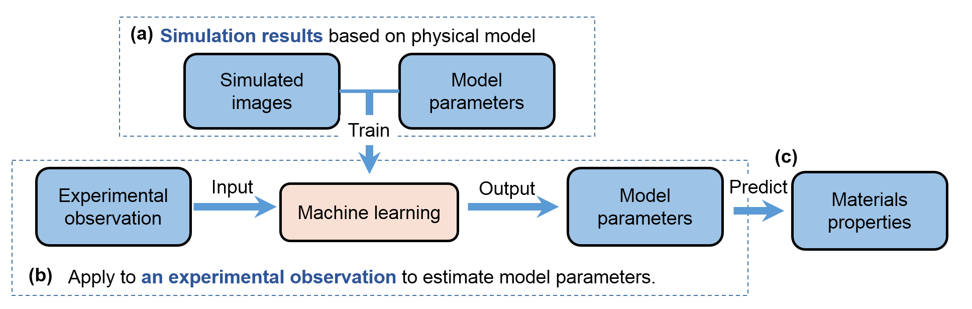
Figure 1: Flow chart of our approach. (a) For a particular experimental observation, a training dataset is formed using simulated images of different Hamiltonian parameters under the same conditions as the experiment. A machine learning model is trained on these images labeled by the Hamiltonian parameters, and consequently is capable to estimate Hamiltonian parameters from a new image. (b) An experimental observation is input into the well trained machine learning model, which outputs the corresponding Hamiltonian parameters of that observation. (c) The estimated Hamiltonian parameters can then be used to predict the properties of material.

Machine learning (ML) algorithms, such as tree based models Clark and Pregibon (2017), kernel based regressors Xue et al. (2016), and artificial neural networksCarrasquilla and Melko (2017); van Nieuwenburg et al. (2016); Rem et al. (2019); Zhang et al. (2019); Carleo and Troyer (2016); Bohrdt et al. (2019); Greplova et al. (2017); Valenti et al. (2019), learn from the labeled data and predict the unexplored search space, providing a prevalent tool in condensed-matter research. Examples of this include learning the phases and phase transitions of matters Ch’ng et al. (2017); Carrasquilla and Melko (2017); van Nieuwenburg et al. (2016); Rem et al. (2019); Zhang et al. (2019), solving the quantum many-body problems Carleo and Troyer (2016),classifying the snapshots of ultracold atoms Bohrdt et al. (2019), and estimating quantum parameter from quantum measurement Greplova et al. (2017); Valenti et al. (2019). Given the success of machine learning in the classification problems in the examples above, the next challenge is to quantitatively extract the physical model parameters from images, especially from experimental ones, so that more abundant information can be obtained. To do so, the most severe obstacle is the insufficient labeled experimental data to construct a good ML model.

II. FRAMEWORK

Here we propose an approach based on a combination of numerical simulation and machine learning to achieve parameters estimation from an experimental image . Figure 1 shows the workflow chart of our approach. For a particular experimental observation, we simulate images using Hamiltonian parameters under the same conditions as the experiment. A ML model is trained on these images labeled by the Hamiltonian parameters, and consequently is capable to estimate Hamiltonian parameters from a new image. Then an experimental observation is input into the well trained ML model, which outputs the corresponding Hamiltonian parameters of that observation. The estimated Hamiltonian parameters can then be used to predict the properties of material. Our approach allows us to estimate Hamiltonian parameters simultaneously with a single input of experimental observation, without any prior knowledge. We demonstrate the success of our approach by precisely estimating three key magnetic parameters ($A_{ex}$, $DMI$ and $M_{sat}$) from input of a spin configuration observation. The real materials properties such as the hysteresis can then be predicted and validated. Our work provides a new way to perform parameters estimation in an accelerated, accurate, and efficient manner.

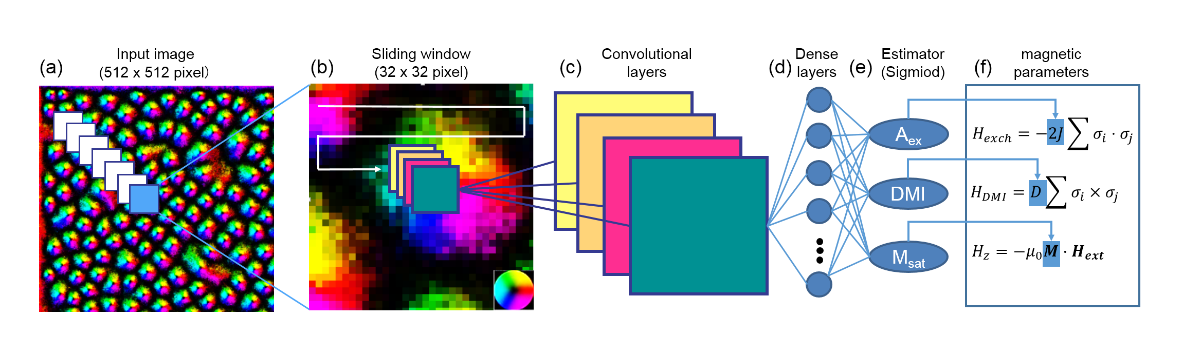
Figure 2: The implementation of a convolutional neural network (CNN) to estimate Hamiltonian parameters from images of spin configuration. (a) Input images of the spin configuration (each pixel represents a spin, the color represents the spin orientation) which are labeled with magnetic parameters of $A_{ex}$, $DMI$, and $M_{sat}$. The sliding window on the input images enlarges the training observations. (b) The slided small windows are inputed to a deep convolutional neural network with a variety of layers including (c) convolutional filters, (d) fully connected layers and (e) a output layer. The output layer is set as a estimator actived by $sigmoid$ to output continuous values of parameters. The three neurons of final sigmoid layer outputs the value of $A_{ex}$, $DMI$, and $M_{sat}$. With those estimated parameters, one can predict materials behaviors and understand underlying physics.

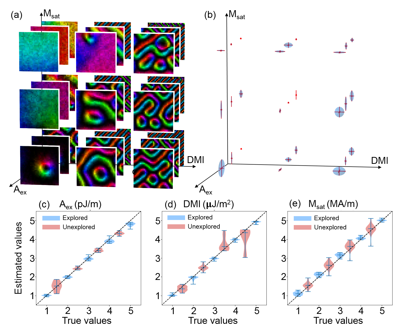
Figure 3: (a) Spin configurations generated by micro-magnetic simulation with the same parameter sets of $A_{ex}$,$DMI$,$M_{sat}$ as the training data but with different initial random seeds. They possess different configurations compared with training data, but contain the same information of parameters. (b) The deviations of estimation for the data of (a) in the parameter space. Error bars in each direction indicate the distance between estimation and the true values of the parameters. (c-e) Plots of the estimated values as the function of true values of the $A_{ex}$,$DMI$,$M_{sat}$ respectively. The blue ones are parameters used in the training data while the red ones represent parameters which are absent in the training data.

III. EXPERIMENT

The Hamiltonian parameters we focus on here are three key parameters ($A_{ex}$, $DMI$ and $M_{sat}$) of a magnetic system. We combines micro-magnetic simulation together with a convolutional neural network (CNN) to perform the estimation process as shown in Figure 1.

The first stage is the preparation of the training dataset for CNN. The dataset presumably contains images of spin configurations and their corresponding magnetic parameters, as shown in Figure 2(a), respectively. However, collecting such a dataset experimentally still remains challenging as it is prohibitively laborious and expensive. Borrowed the idea from transfer learning of the robot trainingChebotar et al. (2019), we generate a training dataset containing simulated spin configurations under a particular temperature and an external field by micro-magnetic model together with the magnetic parameters used. Robustness of the micro-magnetic model allows us to train a CNN that can be adapted to experimental results. To reduce the time cost of the simulation, we simulate monolayer sample to approximate thin film sample or thin specimen used during the transmission electron microscope observation. But the idea is general and can be extended to more complex situations.

In the second stage, a CNN architecture is established, which consists of convolutional layers and dense layers as shown in Figure 2(c) and (d), respectively. Unlike the traditional CNN that directly input the image to the convolutional layers, we introduce a data augmentation method of the sliding window to generate more input data on a small amount of simulated images before the convolutional layer, as shown in Figure 2(a) to (b). An advantage of the physical system comparing to the inputs of conventional image processing is that the underlying information is distributed evenly, i.e., any part of the image contains the same information from one set of model parameters. Thus we cut many portions of the input image by sliding the window, which serve as training images with their parameters known. This step greatly enlarges our training dataset and consequently leads to a better CNN. Moreover, we replace the last layer of conventional CNN (usually a classifier) with an estimator by changing the active function from $softmax$ to $sigmoid$. Doing so enables the CNN to estimate continuous values, as shown in Figure 2(e). Specifically, the estimator layer includes three nodes, and each node will output a value of a particular magnetic parameter of $A_{ex}$, $DMI$ and $M_{sat}$. By utilizing the trained CNN, these parameters for a particular spin configuration can be extracted, and then the prediction of materials properties or the understanding of physics of magnetic phenomena by models such as micro-magnetic simulation can be performed, as shown by Figure 1(b) to (c).

The performance of our CNN model is then evaluated with simulated test data and real experimental images, respectively. As shown in Figure 3, our CNN model performs well for the testing data set which are generated by micro-magnetic simulation but have not appeared in the training process. Figure 3(a) shows a set of simulated spin configurations that are different from our training data but generated using the same set of magnetic parameters as the training spin configuration. The random initial seeds are different, thus different spin configurations are obtained. Their magnetic parameters of $A_{ex}$, $DMI$, and $M_{sat}$ are estimated by our CNN model with the inputs in Figure 3(a) and are shown in the parameter space in Figure 3(b). The size of the ellipsoid indicates the deviation of the estimated values from the true ones. The estimation of $A_{ex}$ is very good, and deviations of $DMI$ and $M_{sat}$ are slightly larger but still within an acceptable level. The estimated values are then plotted as a function of the true values, as shown in Figure 3(c) - (e) by blue violins. The data distribute along the diagonal line, indicating a precise estimation. To test whether our CNN model can estimate parameters that are absent in the training dataset, we generate 4$\times$4$\times$4 new spin configurations. Both the configurations and parameters are absent in the training dataset. Thus we consider those parameters are unexplored ones. As shown in Figure 3(c) - (e) by pink violins, the unexplored parameters are also around the diagonal line, revealing the robustness of our CNN.

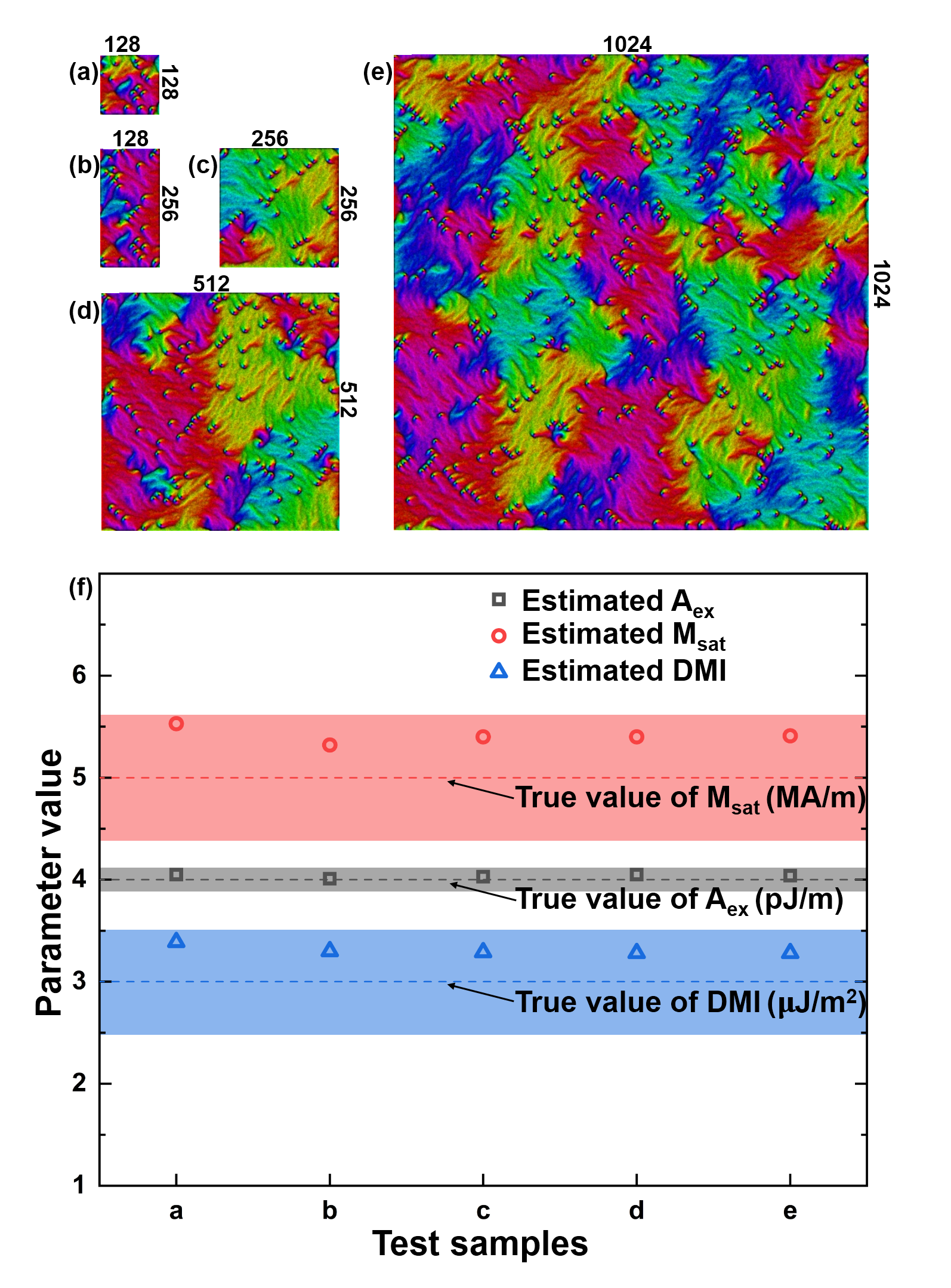
Figure 4: (a-e) Spin configurations from micro-magnetic simulation with the same values of $A_{ex}$, $DMI$, and $M_{sat}$, but different image sizes of 128$\times$128, 128$\times$256, 256$\times$256, 512$\times$512, and 1024$\times$1024. (f) The estimated parameter values from images of different sizes shown in (a-e). The relative error for $A_{ex}$ is less than 2%, and that for $DMI$ and $M_{sat}$ is around 10%.

The above testing result has proved the forecasting capability of our CNN, which is achieved by learning patterns from spin configurations rather than similarity measurement or remember the spin configurations. As the experimental observation varies in size, the generalization ability of our CNN to any size of image is of importance. To validate such an ability, we can estimate the parameters from input images with different sizes rather only the size of $512\times 512$ used in our training data. We generate 5 images of different sizes from the same set of parameters as shown in Figure 4(a) - (e). Noted that the morphology of spin configurations depends on the sample size.Mulkers et al. (2016) Figure 4(f) plots the estimated values from different inputs, comparing with the true ones. It can be seen that the CNN performs well regardless of the size of the input image.

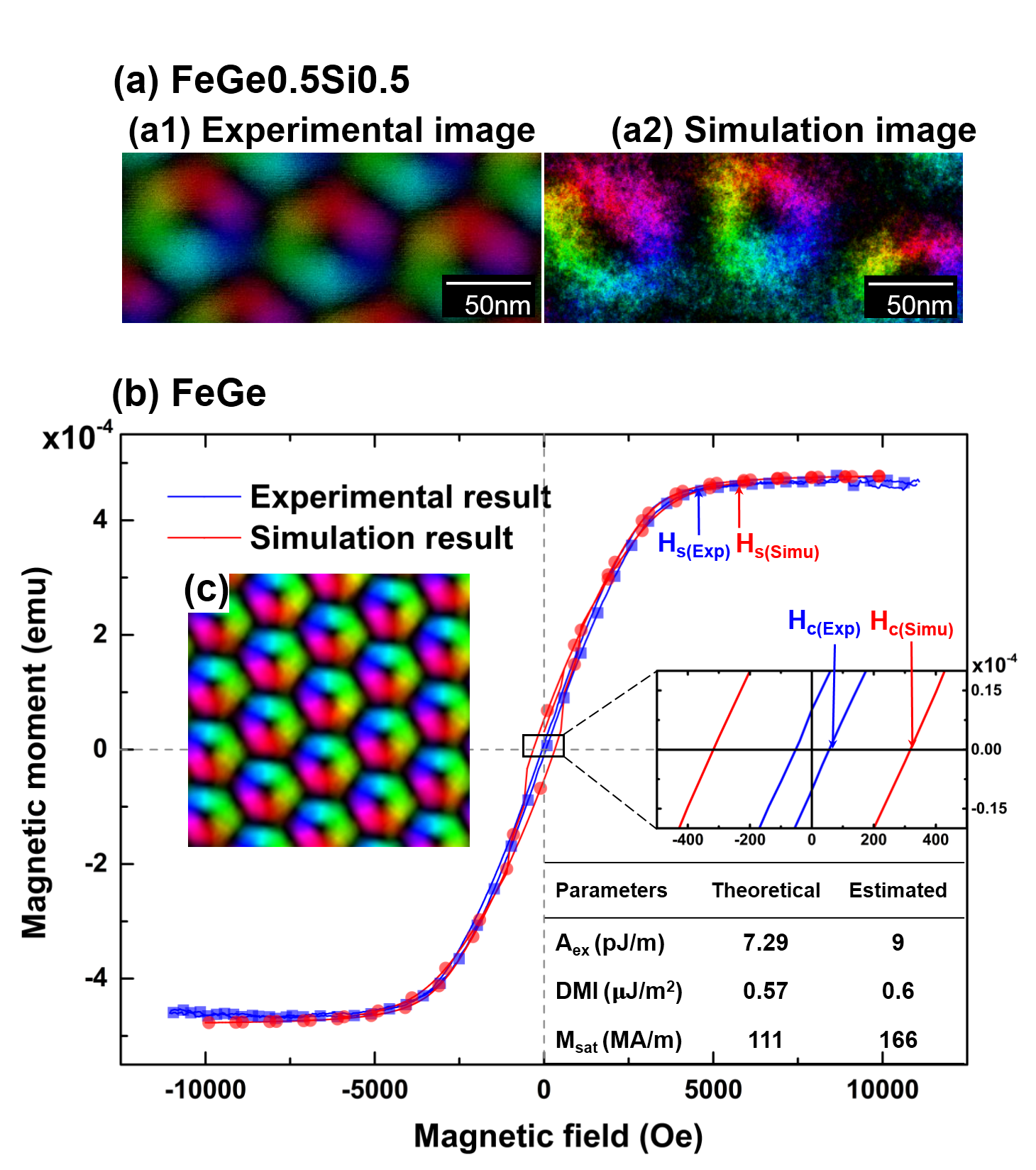
Figure 5: (a) The comparison of spin configurations between the experimental imageMatsumoto et al. (2016) (input to our CNN) and the simulated image using estimated parameters by our CNN. (b) Inputing the spin configurationEsser (2018) shown in (c) to our CNN, the parameters are estimated and comparable to the theoretical valuesTakagi et al. (2017) as shown in the inset table. The hysteresis loop predicted by the micro-magnetic simulation using these estimated values is in agreement with the experimental oneHuang and Chien (2012). The saturation field $H_{s}$ is defined at the knee point in the M-H curve. The coercive field $H_{c}$ is defined at the intersection point between loop and x axis.

With the power of estimating parameters from input images of various sizes with different parameter sets, a key advantage of our CNN is its ability to be directly adapted to real experimental image. We chose FeGe Esser (2018) and FeGe_0.5Si_0.5 Matsumoto et al. (2016) as examples to validate our CNN model. These materials are of great interest due to the existence of the topological phase of skyrmions. We follow the workflow in Figure 1 to estimate three intrinsic parameters of $A_{ex}$, $DMI$, and $M_{sat}$. For each case of the two experimental observations, we generate a training dataset utilizing the same temperature and magnetic field used in the experiment to train a CNN following the implementation shown in Figure 2. As we have the sliding window step, we do not need to generate a large amount of training data and consequently the process is rather efficient. The results of two examples are shown in Figure 5. An experimental skyrmion lattice of FeGe_0.5Si_0.5 specimen by Lorentz transmission electron microscope (TEM) image reconstruction is shown in Figure 5(a1). The observation is performed at 95K under 160mT. Although the nominal composition of Si is 0.5, the actual composition is hard to determine and thus a precise estimation of parameters of this material is not an easy task. We generate a training dataset with 5$\times$5$\times$5 spin configurations by micro-magnetic simulation at temperature of 95 K and under magnetic field of 160 mT. A CNN model is trained on this dataset and estimates the magnetic parameters of $A_{ex}$, $DMI$, and $M_{sat}$ by inputing the experimental skyrmion lattice shown in Figure 5(a1). The spin configuration then can be reproduced from the micro-magnetic simulation using the estimated parameters, and the result is shown in Figure 5(a2). The reproduced configuration exhibits very similar features with the experimental observation, indicating a good estimation of these magnetic parameters.

Besides reproducing the spin configuration, it is also possible to predict the macroscopic properties of a material from only an experimental observation. A skyrmion lattice of FeGe thin film is shown in Figure 5(c). It is observed by Lorentz TEM at 265 K under 0.18 T. Adaptively, we generate 5$\times$5$\times$5 spin configurations by micro-magnetic simulation using temperature of 265 K and magnetic field of 0.18 T and train a new CNN to perform the estimation. As shown in the inset table of Figure 5(b), the estimated parameters are in agreement with the theoretical values for this kind of material, which are obtained by microwave absorption spectroscopy. Takagi et al. (2017) We further predict the hysteresis loop of FeGe at the observation temperature 265 K. The coercive field ($H_{c}$) and saturation field ($H_{s}$) of the predicted hysteresis loop, which are intensive properties of material, are in agreement with the experimental result Huang and Chien (2012) as shown in Figure 5(b). Since we are not able to get access to the volume of the experimental sample, we vary the sample volume in our simulation to fit the experimental value of the magnetic moment, which is an extensive property. So that we can estimate the actual volume of the experimental sample around $1mm\times 1mm\times 3nm$, which is reasonable for a SQUID measurement. Here we employ such an adaptive strategy to train CNN that apply to the particular parameters estimation problems. However, it is possible to include the temperature and magnetic field as the tuning parameters, which requires “big data” to train, so that the trained CNN can be more general and applied to any experimental observations directly.

IV. DISCUSSION

The mapping between the spin configurations and magnetic parameters are rather complex, for example, there are infinite possible configurations from one set of parameters due to the fluctuations and initial randomness. Traditionally, the manually designed descriptors to the spin configuration could inevitably loss part of useful information, which makes the estimation of parameters hard. The CNN which automatically designs as many descriptors of the spin configures as possible and extracts the most relevant features, is so far the best approach to handle this complex mapping problem. The above validations shows that it is rather possible to acquire magnetic parameters from the spin configuration by a CNN machine learning model.

The key ingredients of our approach include: 1) to overcome the shortage of well labeled experimental data, we train a CNN on a small training data with images generated by micro-magnetic simulation, which is adaptable to a particular experimental observation with certain condition such as sample shape, temperature, field, and resolution; 2) we propose a data augmentation method: sliding initial image to effectively enlarges the number of input images as the information of parameters distributed evenly throughout the whole spin configuration; and 3) setting the last layer of CNN to be an estimator for continuous values instead of the classifier for discrete ones.

V. CONCLUSION

In summary, we demonstrate a direct and efficient estimation of magnetic parameters from a single observation of spin configuration via combination of numerical simulation and machine learning. Specifically, we demonstrate how to estimate targeted magnetic parameters via machine learning from only a single experimental image without any other experimental inputs. Such an adaptive feature of our approach allows us to deploy it to various experimental observations under different conditions to estimate magnetic parameters, which are usually lack of enough labeled data. The estimated parameters together with numerical simulations based on Hamiltonian of that system can provide many information of the system, such as the micrographies, macroscopic properties, the phase diagram Yu et al. (2010) and so on. It is thus likely to accelerate the discovery of new materials such as skyrmions with the help of these predictions. Our approach provides a new paradigm to bridge theoretical Hamiltonian to the real material using the combination of numerical simulation and machine learning. It can be generalized to other condensed matter systems whose microstructure and properties can be described by a Hamiltonian.

Appendix

.1 Micro-magnetic simulation

A GPU-accelerated micro-magnetic simulation program, $MuMax^{3}$, generates spin configurations under different parameter sets and with different initial magnetization seeds Vansteenkiste et al. (2014).

For the studies in Figure 3, the environment parameters and geometry parameters have been set as:

Figure 6: Illustration of our data used. Blue blocks represent training data, which are generated with an initial magnetization seed 1. Green blocks represent test_A data, which has the same magnetic parameters as the training data but with an initial magnetization seed 2. Yellow blocks represent test_B data, which are generated from unexplored magnetic parameters.

To generate the training data, magnetic parameters are set as $A_{ex}$=1,2,3,4,5 $(pJ/m)$, $DMI$=1,2,3,4,5 $\left(\bm{\mu}\mathrm{J}/\mathrm{m}^{2}\right)$ and $M_{sat}$=1,2,3,4,5 $(\mathrm{MA}/\mathrm{m})$. In total, there are 125 parameter sets. And 125 spin configurations under these parameter sets with an initial magnetization seed 1 are generated, as shown by blue color label $train$ in Figure 6.

In order to test, we first generate test_A dataset, which includes 125 spin configurations under the parameter sets having been explored before, with an initial magnetization seed 2 as shown by green color label in Figure 6. Furthermore, we generate test_B dataset, which contains 64 spin configurations under parameter sets of $A_{ex}$ = (1.5,2.5,3.5,4.5), $DMI$ = (1.5,2.5,3.5,4.5) and $M_{sat}$ = (1.5,2.5,3.5,4.5), which are not explored by the CNN yet, as shown by yellow color label in Figure 6.

In the experimental image estimation part, the environment parameters and geometry parameters have been set the same as the observation conditions.

.2 Convolutional Neural Network

Table 1: Convolutional Neural Network Architecture

Layer	Layer name	Layer function	Layer description
1	original image	Image input	512*512*3 image of PNG format
2	overlapping sliding window	Cut image	window size:32*32 sliding step size:8
3	conv-1	Convolution	64 3*3*3 convolutions with strides
4	relu-1	Relu	Rectified-linear unit layer
5	padding-1	Padding	Zero padding
6	maxpooling	Maxpooling	Maxpooling
7	dropout-1	Dropout	25$\%$ dropout
8	conv-2	Convolution	128 3*3*64 convolutions with strides
9	relu-2	Relu	Rectified-linear unit layer
10	padding-2	Padding	Zero padding
11	dropout-2	Dropout	25$\%$ dropout
12	fc-1	Fully connected	fc layer with 512 neurons
13	fc-2	Fully connected	fc layer with 64 neurons
14	dropout-3	Dropout	50$\%$ dropout
15	sigmoid	Sigmoid	Sigmoid
16	estimator	Estimation output	MSE Loss

As our input data contains parameters information homogeneously, we employ overlapping sliding window to enlarge our data. We have studied a variety of data augmentation methods and found that only the sliding window works on the spin configuration. Other methods such as scaling and rotation will change the meaning of spin configurations. We have found the overlapping sliding window method is better than the non-overlapping sliding windows, and the best window size equals to 32 and the best slide step size equals to 8. Such a setting can help CNN perform well while keeping the CNN small and easy to train. Motivated by the success of CNN in image recognition, we employ convolutional layers to extract parameters information by feature maps. We have studied a variety of network architectures and found that convolutional neural networks have much better performance than fully connected networks with the same number of layers. To achieve the estimation task, we apply the last layer a sigmoid activation function. The detailed architecture is defined in Table 1.

During training, the parameters of the CNN are adjusted iteratively to minimize a cost function of mean-square-error (MSE). Stochastic gradient descent, along with back propagation, is used for lowering the cost function. The training is stopped and all parameters of CNN are set when the MSE saturates.

.3 Experimental image

The experimental image of FeGe Esser (2018) is kindly provided by Dr. Esser and that of FeGe_0.5Si_0.5 Matsumoto et al. (2016) is kindly provided by Dr. Matsumoto. FeGe spin configuration is observed at 265 K under 50 mT, and the resolution is 2.34 nm/pixel. FeGe_0.5Si_0.5 one is observed at 95 K under 160 mT, and the resolution is 0.54 nm/pixel. The experimental hysteresis of FeGe Huang and Chien (2012) is kindly provided by Dr. Huang, and it is measured under 250K.

References

- Cartwright (1983) N. Cartwright, How the laws of physics lie (1983).
- Burgess et al. (2013) J. A. Burgess, A. E. Fraser, F. F. Sani, D. Vick, B. D. Hauer, J. P. Davis, and M. R. Freeman, Science 339, 1051 (2013).
- Leliaert et al. (2018) J. Leliaert, M. Dvornik, J. Mulkers, J. De Clercq, M. Milošević, and B. Van Waeyenberge, Journal of Physics D: Applied Physics 51, 123002 (2018).
- Thiaville et al. (2002) A. Thiaville, J. M. Garcı́A, and J. Miltat, Journal of Magnetism & Magnetic Materials 242, 1061 (2002).
- Sampaio et al. (2013) J. Sampaio, V. Cros, S. Rohart, A. Thiaville, and A. Fert, Nature Nanotechnology 8, 839 (2013).
- Zhou et al. (2015) Y. Zhou, E. Iacocca, A. A. Awad, R. K. Dumas, F. C. Zhang, H. B. Braun, and J. Åkerman, Nature Communications 6, 8193 (2015).
- Farhan et al. (2013) A. Farhan, P. M. Derlet, A. Kleibert, A. Balan, R. V. Chopdekar, M. Wyss, L. Anghinolfi, F. Nolting, and L. J. Heyderman, Nature Physics 9, 375 (2013).
- Ramirez et al. (1999) A. P. Ramirez, A. Hayashi, R. J. Cava, R. Siddharthan, and B. S. Shastry, Nature 399, 333 (1999).
- Wang et al. (2006) R. F. Wang, C. Nisoli, R. S. Freitas, J. Li, W. Mcconville, B. J. Cooley, M. S. Lund, N. Samarth, C. Leighton, and V. H. Crespi, Nature 439, 303 (2006).
- Ladak et al. (2010) S. Ladak, D. E. Read, G. K. Perkins, L. F. Cohen, and W. R. Branford, Nature Physics 6, 359 (2010).
- Tchernyshyov (2010) O. Tchernyshyov, Nature Physics 6, 323 (2010).
- Zhang and Sarovar (2014) J. Zhang and M. Sarovar, Physical review letters 113, 080401 (2014).
- Eyrich et al. (2012) C. Eyrich, W. Huttema, M. Arora, E. Montoya, F. Rashidi, C. Burrowes, B. Kardasz, E. Girt, B. Heinrich, O. Mryasov, et al., Journal of Applied Physics 111, 07C919 (2012).
- Buford et al. (2016) B. Buford, P. Dhagat, and A. Jander, IEEE Magnetics Letters PP, 1 (2016).
- Burgarth and Ajoy (2017) D. Burgarth and A. Ajoy, Phys. Rev. Lett. 119, 030402 (2017).
- Clark and Pregibon (2017) L. A. Clark and D. Pregibon, in Statistical models in S (Routledge, 2017) pp. 377–419.
- Xue et al. (2016) D. Xue, P. V. Balachandran, J. Hogden, J. Theiler, D. Xue, and T. Lookman, Nature communications 7, 11241 (2016).
- Carrasquilla and Melko (2017) J. Carrasquilla and R. G. Melko, Nature Physics (2017).
- van Nieuwenburg et al. (2016) E. van Nieuwenburg, Y. H. Liu, and S. Huber, Nature Physics (2016).
- Rem et al. (2019) B. S. Rem, N. Käming, M. Tarnowski, L. Asteria, N. Fläschner, C. Becker, K. Sengstock, and C. Weitenberg, Nature Physics 15, 917 (2019).
- Zhang et al. (2019) Y. Zhang, A. Mesaros, K. Fujita, S. Edkins, M. Hamidian, K. Ch’ng, H. Eisaki, S. Uchida, J. S. Davis, E. Khatami, et al., Nature 570, 484 (2019).
- Carleo and Troyer (2016) G. Carleo and M. Troyer, Science 355, 602 (2016).
- Bohrdt et al. (2019) A. Bohrdt, C. S. Chiu, G. Ji, M. Xu, D. Greif, M. Greiner, E. Demler, F. Grusdt, and M. Knap, Nature Physics 15, 921 (2019).
- Greplova et al. (2017) E. Greplova, C. K. Andersen, and K. Mølmer, arXiv preprint arXiv:1711.05238 (2017).
- Valenti et al. (2019) A. Valenti, E. van Nieuwenburg, S. Huber, and E. Greplova, arXiv preprint arXiv:1907.02540 (2019).
- Ch’ng et al. (2017) K. Ch’ng, J. Carrasquilla, R. G. Melko, and E. Khatami, Phys. Rev. X 7, 031038 (2017).
- Chebotar et al. (2019) Y. Chebotar, A. Handa, V. Makoviychuk, M. Macklin, J. Issac, N. Ratliff, and D. Fox, in 2019 International Conference on Robotics and Automation (ICRA) (IEEE, 2019) pp. 8973–8979.
- Mulkers et al. (2016) J. Mulkers, M. V. Milošević, and B. V. Waeyenberge, Phys.rev.b 93, 214405 (2016).
- Matsumoto et al. (2016) T. Matsumoto, Y. G. So, Y. Kohno, H. Sawada, Y. Ikuhara, and N. Shibata, Science Advances 2, e1501280 (2016).
- Esser (2018) B. D. Esser, High Resolution Characterization of Magnetic Materials for Spintronic Applications, Ph.D. thesis, The Ohio State University (2018).
- Takagi et al. (2017) R. Takagi, D. Morikawa, K. Karube, N. Kanazawa, K. Shibata, G. Tatara, Y. Tokunaga, T. Arima, Y. Taguchi, Y. Tokura, and S. Seki, Phys. Rev. B 95, 220406 (2017).
- Huang and Chien (2012) S. X. Huang and C. L. Chien, Physical Review Letters 108, 267201 (2012).
- Yu et al. (2010) X. Z. Yu, . Onose, Y., . Kanazawa, N., J. H. Park, J. H. Han, . Matsui, Y., . Nagaosa, N., and . Tokura, Y., Nature 465, 901 (2010).
- Vansteenkiste et al. (2014) A. Vansteenkiste, J. Leliaert, M. Dvornik, F. Garcia-Sanchez, and B. V. Waeyenberge, Aip Advances 4, 323001 (2014).