Invariant Synchrony Subspaces of Sets of Matrices

Abstract.

A synchrony subspace of $\mathbb{R}^{n}$ is defined by setting certain components of the vectors equal according to an equivalence relation. Synchrony subspaces invariant under a given set of square matrices ordered by inclusion form a lattice. Applications of these invariant synchrony subspaces include equitable and almost equitable partitions of the vertices of a graph used in many areas of graph theory, balanced and exo-balanced partitions of coupled cell networks, and coset partitions of Cayley graphs. We study the basic properties of invariant synchrony subspaces and provide many examples of the applications. We also present what we call the split and cir algorithm for finding the lattice of invariant synchrony subspaces. Our theory and algorithm is further generalized for non-square matrices. This leads to the notion of tactical decompositions studied for its application in design theory.

1. Introduction

Invariant subspaces of matrices play an important role in many areas of mathematics [24]. We study a special type of invariant subspace, the invariant synchrony subspace where certain components are equal, and further generalize this notion by considering invariance with respect to more than one matrix. These invariant synchrony subspaces come from certain partitions of the components, which we call invariant partitions. Invariant partitions have a surprisingly large number of applications and have been studied, often in different form, in graph theory, network theory, mathematical biology, and other areas of mathematics. For example, they relate to almost equitable partitions, coupled cell networks, dynamical systems, network controllability, and differential equations. Our own interest in the subject initiated from needing to understand all possible bifurcations for a given family of semilinear elliptic PDE, including cases where symmetry did not fully describe the invariant spaces. In that research it became apparent that what we called anomalous invariant subspaces can occur quite frequently, and must be understood in order to robustly and efficiently find and follow new branches of solutions with local symmetry. Thus, it is desirable to be able to find all invariant partitions, which form a lattice. Our main contribution is the split and cir algorithm that finds this lattice relatively well, by which we mean it has some efficiencies that allow a modestly large calculation, and for multiple matrices. A secondary goal of this article is to provide a common framework that brings together different areas of research so that we can better share results.

There are a number of papers that describe algorithms for finding the coarsest invariant partitions for a single matrix [6, 8, 9]. These algorithms were developed for algebraic graph theory and are often described in graph theoretic terminology (e.g., vertex degree). For example, this is used for the graph isomorphism problem in Nauty [32].

Our cir algorithm is a slight generalization of these algorithms. It finds the coarsest invariant refinement of a given partition for a set of matrices. The coarsest invariant partition is the cir of the singleton partition. Our implementation of cir was inspired by [22, 48]. By recursively splitting classes of an invariant partition and finding the cir of each of these finer partitions, we compute the lattice of invariant partitions. This provides us with a relatively efficient split and cir algorithm for the NP-complete problem of finding the lattice of invariant partitions. The recursive combination of cir with class splitting is the main contribution of our paper.

Our algorithm is close to that of [27]. They find the lattice of invariant partitions by finding the coarsest invariant partition and then check every finer partition by brute force. We believe that our split and cir algorithm with the recursive application of cir is more efficient, allowing for larger calculations.

By quite different means toward a similar end, the cell network results of [1] use eigenvectors of each individual adjacency matrix after dividing the network into regular subnetworks. We believe that our algorithm is more numerically stable since it uses integer arithmetic.

We generalize our split and cir algorithm a bit further to allow non-square matrices. This handles a possibly generalized notion (more than one matrix) of tactical decompositions used in design theory.

The organization of the paper is as follows. In Section 2 we make some definitions and examples concerning the partial ordering of partitions. We define synchrony subspaces in Section 3, where we give some useful facts concerning the lattice of partitions. In Section 4 we define invariant synchrony subspaces for collections of matrices, and show that invariant partitions form a lattice. Applications of invariant synchrony subspaces are provided in Section 5. We feature equitable and almost equitable partitions of graphs, balanced and exo-balanced partitions of coupled cell networks, weighted cell network systems, network controllability, Cayley graphs, and finite difference methods for PDE. The invariant subspaces for all of these applications can be treated in terms of invariant partitions for the appropriate collection of matrices. Section 6 provides some technical tools needed for the cir algorithm, which is developed in Section 7. We provide the split and cir algorithm for computing the lattice of invariant partitions in Section 8. We parallel this development for non-square matrices with applications to tactical decompositions in Sections 9, 10, and 11.

2. Preliminaries

We recall some terminology and notation for partially ordered sets. Our general reference is [26]. A set $P$ with a relation $\leq$ is a partially ordered set or poset if the relation is reflexive, antisymmetric, and transitive. The down-set of an element $x$ of $P$ is

$$\downarrow x:=\{y\in P\mid y\leq x\}.$$

A poset $L$ is a lattice if the join $a\vee b:=\sup\{a,b\}$ and meet $a\wedge b:=\inf\{a,b\}$ exist for all $a,b\in L$. Equivalently, $L$ is a lattice if $\bigvee H:=\sup(H)$ and $\bigwedge H:=\inf(H)$ exist for any finite subset $H$ of $L$. A lattice $L$ is called complete if $\bigvee H$ and $\bigwedge H$ exist for any subset $H$ of $L$.

An element $y$ of a poset covers another element $x$ if $x<y$ but $x<z<y$ does not hold for any $z$. We use the notation $x\prec y$ for the covering relation. We also say that $x$ is a lower cover of $y$ and $y$ is an (upper) cover of $x$.

Example 2.1.

The set $L(\mathbb{R}^{n})$ of subspaces of $\mathbb{R}^{n}$ is a poset under reversed containment. It is also a lattice such that $U\vee V=U\cap V$ and $U\wedge V=U+V$.

Example 2.2.

Let $\Pi(n)$ be the set of partitions of the set $\{1,\ldots,n\}$. We are going to simply write $\Pi$ if $n$ is clear from the context. We refer to an element of a partition as an (equivalence) class. The class of $i$ is denoted by $[i]$. A partition $\mathcal{B}$ is coarser than another partition $\mathcal{A}$ if every class of $\mathcal{A}$ is contained in some class of $\mathcal{B}$. Equivalently, $\mathcal{B}$ is coarser than $\mathcal{A}$ exactly when $[i]_{\mathcal{A}}=[j]_{\mathcal{A}}$ implies $[i]_{\mathcal{B}}=[j]_{\mathcal{B}}$ for all $i$ and $j$. In this case we write $\mathcal{A}\leq\mathcal{B}$ and also say that $\mathcal{A}$ is finer than $\mathcal{B}$ or that $\mathcal{A}$ is a refinement of $\mathcal{B}$. The set $\Pi(n)$ with this order forms a lattice [12, Theorem 4.11]. The top element of this lattice is the singleton partition $\{\{1,\ldots,n\}\}$ and the bottom element is the discrete partition $\{\{1\},\ldots,\{n\}\}$. We use the simplified notation for a partition where we list the elements of the classes separated by a bar. So the singleton partition is $12\cdots n$ and the discrete partition is $1|2|\cdots|n$.

A partition $\mathcal{B}$ covers another partition $\mathcal{A}$ if $\mathcal{A}$ can be constructed from $\mathcal{B}$ by splitting one of the classes of $\mathcal{B}$ into two nonempty sets. More precisely, we have the following.

Proposition 2.3.

For $\mathcal{A},\mathcal{B}\in\Pi(n)$, $\mathcal{A}\prec\mathcal{B}$ if and only if $\mathcal{B}=\mathcal{A}\cup\{A\cup B\}\setminus\{A,B\}$ for some $A,B\in\mathcal{A}$.

3. Synchrony subspaces

The characteristic vector of a subset $C$ of $\{1,\ldots,n\}$ is the vector $(x_{1},\ldots,x_{n})$ such that $x_{i}=1$ for $i\in C$ and $x_{i}=0$ for $i\not\in C$. The characteristic matrix of a partition $\mathcal{A}=\{C_{1},\ldots,C_{k}\}\in\Pi(n)$ is the matrix $P(\mathcal{A})$ whose columns are the characteristic vectors of the classes of $\mathcal{A}$. The classes of $\mathcal{A}$ are ordered lexicographically and the characteristic vectors are listed in the same order. The coloring vector of $\mathcal{A}$ is $c(\mathcal{A}):=(c_{1},\ldots,c_{n})$ such that $i\in C_{c_{i}}$ for all $i\in V$. Note that $P(\mathcal{A})$ is the $n\times|\mathcal{A}|$ matrix with components $P(\mathcal{A})_{i,a}=\delta_{c_{i},a}$. We use the identification $\mathbb{R}^{n}\equiv\mathbb{R}^{n\times 1}$, so the coloring vector $c(\mathcal{A}_{k})$ is also a column matrix.

The set of all coloring vectors is linearly ordered by the lexicographic order. If $\mathcal{A\prec\mathcal{B}}$ then $c(\mathcal{A})<c(\mathcal{B})$ since one of the colors in the class that splits must increase. Hence the coloring vector map is order preserving. That is, $\mathcal{A}\leq\mathcal{B}$ implies $c(\mathcal{A})\leq c(\mathcal{B})$. However the converse is not true. For example $c(12|3)=(1,1,2)<(1,2,2)=c(1|23)$ even though the partitions $12|3$ and $1|23$ are not comparable. We usually order a list of partitions according to the lexicographical order of their coloring vectors. Thus, the first partition in $\Pi(n)$ is the singleton partition $\mathcal{A}_{1}$ with coloring vector $(1,1,1,\ldots,1)$ and the last partition is the discrete partition $\mathcal{A}_{B_{n}}$ with coloring vector $(1,2,3,\ldots,n)$, where $B_{n}$ is the $n$-th Bell number.

Definition 3.1.

For $\mathcal{A}\in\Pi(n)$ we define

$$\operatorname{sys}(\mathcal{A}):=\{(x_{1},\ldots,x_{n})\mid x_{i}=x_{j}\text{ if }[i]=[j]\}\subseteq\mathbb{R}^{n}$$

to be the synchrony subspace of $\mathcal{A}$.

The connection between $\operatorname{sys}(\mathcal{A})$ and $\Delta_{\mathcal{A}}^{P}$ defined for coupled cell networks is discussed in Subsection 5.2. The following is an easy consequence of the definitions.

Proposition 3.2.

The synchrony subspace $\operatorname{sys}(\mathcal{A})$ of a partition $\mathcal{A}$ is the column space $\operatorname{Col}(P(\mathcal{A}))$ of the characteristic matrix $P(\mathcal{A})$.

Example 3.3.

Consider the partitions $\mathcal{A}=12|3$ and $\mathcal{B}=1|23$. The characteristic matrices are

$$P(\mathcal{A})=\left[\begin{smallmatrix}1&0\\ 1&0\\ 0&1\end{smallmatrix}\right],\qquad P(\mathcal{B})=\left[\begin{smallmatrix}1&0\\ 0&1\\ 0&1\end{smallmatrix}\right],$$

the coloring vectors are $c(\mathcal{A})=(1,1,2)$ and $c(\mathcal{B})=(1,2,2)$ while the synchrony subspaces are $\operatorname{sys}(\mathcal{A})=\{(a,a,b)\mid a,b\in\mathbb{R}\}$ and $\operatorname{sys}(\mathcal{B})=\{(a,b,b)\mid a,b\in\mathbb{R}\}$.

The following is an easy consequence of the definitions. See for example [49, Equation (4)].

Proposition 3.4.

The mapping $\operatorname{sys}:\Pi(n)\to L(\mathbb{R}^{n})$ is an order embedding. That is, it is injective and $\mathcal{A}\leq\mathcal{B}$ if and only if $\operatorname{sys}(\mathcal{A})\supseteq\operatorname{sys}(\mathcal{B})$.

We recall another relevant result.

Proposition 3.5.

[48, Lemma 2] If $S\subseteq\Pi(n)$ then $\operatorname{sys}(\bigvee S)=\bigcap\{\operatorname{sys}(\mathcal{A})\mid\mathcal{A}\in S\}$.

4. Invariant synchrony subspaces

A subspace $U$ of $\mathbb{R}^{n}$ is invariant under a matrix $M$ in $\mathbb{R}^{n\times n}$ if $MU=\{Mu\mid u\in U\}$ is a subset of $U$. The subspace $U$ is invariant under a collection $\mathcal{M}$ of matrices if $U$ is invariant under each $M$ in $\mathcal{M}$.

Definition 4.1.

Let $\mathcal{M}\subseteq\mathbb{R}^{n\times n}$. A partition $\mathcal{A}$ in $\Pi(n)$ is called $\mathcal{M}$-invariant if the synchrony subspace of $\mathcal{A}$ is $M$-invariant for all $M\in\mathcal{M}$. That is, $M\operatorname{sys}(\mathcal{A})\subseteq\operatorname{sys}(\mathcal{A})$ for all $M\in\mathcal{M}$. We let $\Pi_{\mathcal{M}}(n)$ be the set of $\mathcal{M}$-invariant partitions. We use the simplified notation $\Pi_{M}(n)$ if $\mathcal{M}=\{M\}$.

Note that $\Pi_{\mathcal{M}}(n)$ is a subposet of $\Pi(n)$.

Example 4.2.

Let

$$M_{1}=\left[\begin{smallmatrix}1&0&0\\ 0&1&0\\ 0&0&2\end{smallmatrix}\right],\quad M_{2}=\left[\begin{smallmatrix}1&0&-1\\ 0&2&0\\ 0&0&0\end{smallmatrix}\right]$$

and $\mathcal{M}=\{M_{1},M_{2}\}$. Then

$$\Pi_{M_{1}}(3) =\{12|3,1|2|3\},$$

$$\Pi_{M_{2}}(3) =\{13|2,1|2|3\},$$

$$\Pi_{\mathcal{M}}(3) =\{1|2|3\}.$$

For example

$$M_{2}\operatorname{sys}(13|2)=\{M_{2}(a,b,a)\mid a,b\in\mathbb{R}\}=\{(0,2b,0)\mid a,b\in\mathbb{R}\}\subseteq\operatorname{sys}(13|2).$$

On the other hand

$$M_{2}\operatorname{sys}(12|3)=\{M_{2}(a,a,b)\mid a,b\in\mathbb{R}\}=\{(a-b,2a,0)\mid a,b\in\mathbb{R}\}\not\subseteq\operatorname{sys}(12|3).$$

Proposition 4.3.

If $\emptyset\neq S\subseteq\Pi_{\mathcal{M}}$ then $\bigvee S\in\Pi_{\mathcal{M}}$.

Proof.

Since $\operatorname{sys}(\mathcal{A})$ is $\mathcal{M}$-invariant for all $\mathcal{A}\in S$, $\operatorname{sys}(\bigvee S)=\bigcap\{\operatorname{sys}(\mathcal{A})\mid\mathcal{A}\in S\}$ is also $\mathcal{M}$-invariant. ∎

Recall the following result.

Proposition 4.4.

[26, Lemma 34] If $P$ is a poset in which $\bigvee S$ exists for all $S\subseteq P$, then $P$ is a complete lattice.

Note that the bottom element of $P$ is $\bigvee\emptyset$, and $\bigwedge S=\bigvee L_{S}$ where $L_{S}$ is the set of lower bounds of $S$. The following is closely related to [1, Section 4].

Proposition 4.5.

If $\mathcal{M}\subseteq\mathbb{R}^{n\times n}$ then $\Pi{}_{\mathcal{M}}(n)$ is a lattice.

Proof.

We verify the conditions of Proposition 4.4. The discrete partition is invariant under any $\mathcal{M}$, so it is the bottom element of $\Pi_{\mathcal{M}}(n)$. Let $\emptyset\neq S\subseteq\Pi_{\mathcal{M}}(n)$ and $\bigvee S$ be the supremum of $S$ taken in the lattice $\Pi(n)$. Then $\bigvee S\in\Pi_{\mathcal{M}}(n)$ by Proposition 4.3. So the supremum of $S$ in $\Pi_{\mathcal{M}}(n)$ is $\bigvee S$. ∎

$\left[\begin{smallmatrix}1&1&0&0&0\\ 1&1&0&0&0\\ 1&1&0&0&0\\ 0&0&1&1&0\\ 0&0&0&1&1\end{smallmatrix}\right]$

$\mathcal{A}_{1}=12345$	$\mathcal{A}_{7}=13|2|4|5$
$\mathcal{A}_{2}=1234|5$	$\mathcal{A}_{8}=14|235$
$\mathcal{A}_{3}=123|4|5$	$\mathcal{A}_{9}=14|23|5$
$\mathcal{A}_{4}=12|3|4|5$	$\mathcal{A}_{10}=1|23|4|5$
$\mathcal{A}_{5}=135|24$	$\mathcal{A}_{11}=1|2|3|4|5$
$\mathcal{A}_{6}=13|24|5$

Figure 4.1. A matrix $M$ and the lattice of $M$-invariant partitions.

	$\mathcal{A}_{5}$	$\mathcal{A}_{8}$	$\mathcal{A}_{5}\wedge\mathcal{A}_{8}$
	balanced	balanced	not balanced

Figure 4.2. Balanced partitions whose infimum in $\Pi$ is not balanced.

Example 4.6.

Figure 4.1 shows a matrix $M$ and the lattice of $M$-invariant partitions. Partitions $\mathcal{A}_{5}=135|24$ and $\mathcal{A}_{8}=14|235$ are $M$-invariant but $\mathcal{A}_{5}\wedge\mathcal{A}_{8}=1|2|35|4$ is not $M$-invariant. The infimum of $\mathcal{A}_{5}$ and $\mathcal{A}_{8}$ in $\Pi_{M}$ is the discrete partition $\mathcal{A}_{11}$. This shows that $\Pi_{\mathcal{M}}$ is not a sublattice of $\Pi$. Although the $\vee$ operation is the same in $\Pi$ and $\Pi_{\mathcal{M}}$, the $\wedge$ operations are not the same. See [1, page 951] and [45]. Note that

$$\operatorname{sys}(\mathcal{A}_{5})+\operatorname{sys}(\mathcal{A}_{8})=\{x\in\mathbb{R}^{5}\mid x_{3}=x_{5},\,x_{1}+x_{2}=x_{3}+x_{4}\}$$

is not a synchrony subspace.

5. Applications

We present several areas of mathematics where invariant synchrony subspaces are used. We introduce the concepts of equitable and almost equitable partitions of graphs. We also talk about balanced and exo-balanced partitions. These are essentially generalizations for colored digraphs. The terminology is still evolving and not completely consistent but generally equitable is used in graph theory and balanced is used for network theory. All of these concepts can be treated as $\mathcal{M}$-invariant partitions for an appropriate $\mathcal{M}$.

5.1. Equitable partitions of graphs

Equitable partitions play an important role in graph theory [22, 23, 31]. They are used for example in algorithms to test if two graphs are isomorphic [32]. Orbits of group actions on graphs form equitable partitions but not all equitable partitions are of this type. Equitable partitions can be used to create quotient digraphs.

If $i$ is a vertex of a digraph, then the neighborhood of $i$ is denoted by $N(i)$. The neighborhood of $i$ consists of the vertices adjacent to $i$. Let $\mathcal{A}$ be a partition of the vertex set of a digraph. The degree of a vertex $i$ relative to the class $B$ is $d_{B}(i):=|N(i)\cap B|$.

Definition 5.1.

A partition $\mathcal{A}$ of the vertex set of a graph is called equitable if $d_{B}(i)=d_{B}(j)$ for all $i,j\in A\in\mathcal{A}$ and $B\in\mathcal{A}$.

Example 5.2.

Every partition of the vertex set of the complete graph $K_{n}$ is equitable since $d_{A}(i)=|N(i)\cap A|=|A|-$1 for all $i\in A$ and $d_{B}(i)=|N(i)\cap B|=|B|$ for all $i\in A\neq B$. So the number of equitable partitions of $K_{n}$ is the Bell number $B_{n}$, which is defined to be the number or partitions of a set with $n$ elements.

Example 5.3.

If $A$ is the adjacency matrix of the graph with vertex set $\{1,\ldots,n\}$, then $\Pi_{A}(n)$ consists of the equitable partitions of the graph [22, Lemma 2.1].

We are going to refer to a directed graph with possible multiple edges and loops as a digraph.

Example 5.4.

$G$		$\mathcal{A}_{1}=124578|36$		$G/\mathcal{A}_{1}$
(i)		(ii)		(iii)

Figure 5.1. (i) Graph $G$. (ii) The coarsest equitable partition $\mathcal{A}_{1}$ of $G$. (iii) The quotient digraph $G/\mathcal{A}_{1}$.

Figure 5.1(ii) shows the coarsest of the eight equitable partitions of the graph $G$ shown in Figure 5.1(i). Figure 5.1(iii) shows the quotient digraph by $\mathcal{A}_{1}$. It is obvious that all orbit partitions under the graph automorphism group are equitable, but the converse is not true. The equitable partition of Figure 5.1(ii) is not an orbit partition. The coarsest orbit partition of $G$ is $1278|36|45$. The full list of equitable partitions for this so-called McKay graph [31, Fig. 5.1] are listed at the companion web site [38].

Note that the coarsest orbit partition of a graph $G$ is always the orbit partition for the natural action of $\operatorname{Aut}(G)$. Furthermore, if $\operatorname{Aut}(G)$ has a vertex with trivial stabilizer subgroup, then the group orbit of that vertex has the same size as that of $\operatorname{Aut}(G)$, and every subgroup of $\operatorname{Aut}(G)$ has a distinct orbit partition. For the graph in Figure 5.1 there is no vertex with trivial stabilizer subgroup, but such a vertex exists for the graphs in the next example.

Example 5.5.

(i)		(ii)		(iii)

Figure 5.2. Equitable partitions. (i) The coarsest equitable partition of $P_{4}\oblong P_{2}$. (ii) The coarsest equitable partition of $P_{4}\oblong P_{4}$ . (iii) The orbit partition of the $\mathbb{Z}_{4}$ action on ${\normalcolor P_{4}\oblong P_{4}}$.

Figure 5.2 shows a few equitable partitions of the $m\times n$ square grid graphs $P_{m}\oblong P_{n}$. We have computed the equitable partitions up to $m=n=20$, along with some larger graphs. The companion web site [38] shows the equitable partitions for several sizes. Unlike the graph in Figure 5.1, it appears that all of the equitable partitions of $P_{m}\square P_{n}$ are orbit partitions.

Conjecture 5.6.

The equitable partitions of $P_{m}\oblong P_{n}$ are the orbit partitions of natural actions of the subgroups of the automorphism group of the graph. The lattice of equitable partitions is isomorphic to the lattice of subgroups exactly when there is a vertex with trivial stabilizer subgroup. This happens unless $2\leq m=n\leq 3$.

Note that the orbit partitions for $\mathbb{Z}_{4}$ and $D_{4}$ are the same for $P_{2}\oblong P_{2}$ and $P_{3}\oblong P_{3}$. An algorithm using the eigenvectors of the adjacency matrix [1, 27] can possibly be applied symbolically for all $m$ and $n$ to prove this conjecture. Alternatively, the techniques of [Antoneli2] might also provide a proof.

5.2. Balanced partitions of coupled cell networks

Synchrony in coupled cell networks introduced by [46] and refined by [25] provide examples of $\mathcal{M}$-invariant synchrony subspaces. A coupled cell network system is a set of dynamical systems coupled according to the arrows of a digraph. An interesting case is where some or all of the cells have the same internal dynamics, so partial or full synchronization of the cells is possible. Coupled cells are of interest to physicists and biologists [11, 40, 43, 44, 42]. A good mathematical review is [7].

A coupled cell network is formally defined in [25] as a digraph with an equivalence relation on the set $\{1,\ldots,n\}$ of cells and another equivalence relation on the arrows, along with the consistency condition that equivalent arrows have equivalent heads and equivalent tails. Intuitively, two cells are in the same equivalence class if they have the same internal dynamics, and two arrows are in the same equivalence class if they represent couplings of the same type. The equivalence classes of the cells and arrows can be considered as colorings. So a cell network is essentially a digraph with compatible cell and arrow colorings. We use different symbols in our figures to indicate the cell colors, and solid or dashed arrows for the edge colors.

A coupled cell network system defined in [25] on the coupled cell network is an ODE defined by an admissible vector field. To define admissible vector fields, a phase space $P_{i}$ is specified for each cell, and the total phase space is the Cartesian product $P=P_{1}\times\cdots\times P_{n}$ of the cell phase spaces. Given a coupled cell network on the digraph $G$ and a total phase space $P$, the set of all admissible vector fields is $\mathcal{F}_{G}^{P}$, the collection of all vector fields compatible with the structure of the colored graph $G$.

The polydiagonal subspace of a cell partition $\mathcal{A}$ of a cell network system is $\Delta_{\mathcal{A}}^{P}:=\{x\in P\mid x_{i}=x_{j}\mbox{ if }[i]=[j]\}$, see [1, 25, 27, 39, 46]. Note that $\Delta_{\mathcal{A}}^{P}=\operatorname{sys}(\mathcal{A})$ if $P=\mathbb{R}^{n}$. A cell partition $\mathcal{A}$ of a coupled cell network system is polysynchronous if $\Delta_{\mathcal{A}}^{P}$ is invariant under the vector field of the system. A cell partition $\mathcal{A}$ of a coupled cell network is robustly polysynchronous if $\Delta_{\mathcal{A}}^{P}$ is invariant under every vector field in $\mathcal{F}_{G}^{P}$ for all choices of $P$.

The adjacency matrix of a digraph with $n$ vertices is the $n\times n$ matrix $A$ with $A_{i,j}$ equal to the number of arrows from vertex $j$ to vertex $i$. Our adjacency matrix is the in-adjacency matrix, which is the preferred choice for cell networks [1]. In graph theory it is more common to use the out-adjacency matrix, which is the transpose of our $A$.

Example 5.7.

The matrix of Example 4.6 shown in Figure 4.1 is the adjacency matrix of the graph shown in Figure 4.2. The adjacency matrix of the digraph in Figure 5.1(iii) is $\left[\begin{smallmatrix}1&1\\ 3&0\end{smallmatrix}\right]$.

Restricting the cell network to a single edge type creates a monochrome digraph of the cell network. The information about a cell network is encoded by the set $\mathcal{M}$ of adjacency matrices of these monochrome digraphs together with the cell type partition $\mathcal{T}$ determined by the vertex types.

If $i$ is a vertex of a digraph, then the in-neighborhood of $i$ is denoted by $N^{-}(i)$. The in-neighborhood consists of the vertices from which there is an arrow to $i$. The in-neighborhood is called the input set in [46] and subsequent articles. Let $\mathcal{A}$ be a partition of the vertex set of a digraph. The in-degree of a vertex $i$ relative to the class $B$ is $d_{B}^{-}(i):=|N^{-}(i)\cap B|$.

Definition 5.8.

Consider a coupled cell network with cell type partition $\mathcal{T}$. A cell partition $\mathcal{A}$ is called balanced if $\mathcal{A}\leq\mathcal{T}$ and $d_{B}^{-}(i)=d_{B}^{-}(j)$ for all $i,j\in A\in\mathcal{A}$ and $B\in\mathcal{A}$ in every monochrome subgraph.

Example 5.9.

A simple graph has no multiple edges or loops. Such a graph determines a cell network with a single class of vertices and a single class of edges. The adjacency matrix of the cell network is symmetric, in fact, it is the adjacency matrix of the original graph. So the equitable partitions of the graph are exactly the balanced partitions of the corresponding cell network.

The following result is the main reason why balanced partitions are important for cell networks.

Proposition 5.10.

[25, Theorem 4.3] A cell partition of a coupled cell network is robustly polysynchronous if and only if it is balanced.

Note that the choice of the phase space $P$ has no effect on whether a partition is robustly polysynchronous, since being balanced does not depend on $P$. The following is a well-known result, see [1, Remark 2.12].

Proposition 5.11.

The set of balanced partitions of a coupled cell network with set of adjacency matrices $\mathcal{M}$ and cell type partition $\mathcal{T}$ is $\Pi_{\mathcal{M}}\cap\downarrow\mathcal{T}$.

Remark 5.12.

Note that $\Pi_{\mathcal{M}}$ is computed from the arrow-colored digraph, with no need for the cell type partition. If $\mathcal{T}$ is the singleton partition, then $\downarrow\mathcal{T}=\Pi$ and so $\Pi_{\mathcal{M}}\cap\downarrow\mathcal{T}=\Pi_{\mathcal{M}}$.

Example 5.13.

		$13|245$		$13|24|5$		$1|25|3|4$		$1|2|3|4|5$
		$\mathcal{A}_{1}$		$\mathcal{A}_{2}$		$\mathcal{A}_{3}$		$\mathcal{A}_{4}$
(i)		(ii)

    (iii)

Figure 5.3. (i) A coupled cell network. (ii) Balanced partitions. (iii) Lattice of balanced partitions.

Figure 5.3 shows the balanced partitions of a cell network with a single cell type. The cell type partition is $\mathcal{T}=12345$ and the set of adjacency matrices is $\mathcal{M}=\{M_{1},M_{2}\}$ where

$$M_{1}=\left[\begin{smallmatrix}0&0&0&0&0\\ 1&0&0&0&0\\ 0&0&0&0&0\\ 0&0&1&0&0\\ 1&0&0&0&0\end{smallmatrix}\right],\quad M_{2}=\left[\begin{smallmatrix}\begin{smallmatrix}0&0&0&1&0\\ 0&0&0&0&0\\ 0&1&0&0&0\\ 0&0&0&0&0\\ 0&0&0&0&0\end{smallmatrix}\end{smallmatrix}\right].$$

The coarsest $\mathcal{M}$-invariant partition is $\mathcal{A}_{1}=13|245$. This is the partition corresponding to input equivalence [25], since cells 1 and 3 feel one dashed arrow, and cells 2, 3, and 5 feel one solid arrow.

In Example 5.13 the only cell type partitions compatible with the arrow types are the singleton partition and $\mathcal{A}_{1}$, the coarsest $\mathcal{M}$-invariant partition. In both cases, the set of balanced partitions is the same. The next example shows that sometimes the cell type partition $\mathcal{T}$ can effect the set of balanced partitions.

Example 5.14.

		$1|234$ $\mathcal{A}_{1}$		$1|23|4$ $\mathcal{A}_{2}$		$1|24|3$ $\mathcal{A}_{3}$		$1|2|34$ $\mathcal{A}_{4}$		$1|2|3|4$ $\mathcal{A}_{5}$
(i)		(ii)										(iii)		(iv)

Figure 5.4. (i) A coupled cell network with two cell types and two arrow types. (ii) $\mathcal{M}$-invariant partitions. (iii) Lattice of $\mathcal{M}$-invariant partitions, with the balanced partitions for the network circled. (iv) Another coupled cell network with only one cell type and four arrow types, and the same balanced partitions as those of (i).

Consider the coupled cell network shown in Figure 5.4(i). The cell type partition is $\mathcal{T}=12|34$ and the set of adjacency matrices is $\mathcal{M}=\{M_{1},M_{2}\}$, where

$$M_{1}=\left[\begin{smallmatrix}0&1&0&0\\ 0&0&0&0\\ 0&0&0&0\\ 0&0&0&0\end{smallmatrix}\right],\quad M_{2}=\left[\begin{smallmatrix}\begin{smallmatrix}0&0&1&1\\ 0&0&0&0\\ 0&0&0&0\\ 0&0&0&0\end{smallmatrix}\end{smallmatrix}\right].$$

The elements of $\Pi_{\mathcal{M}}(4)$ are shown in Figure 5.4(ii). The input partition, as defined in [25, Definition 2.3], is $\mathcal{A}_{1}$. Note that the input partition $\mathcal{A}_{1}$ is not a refinement of the cell type partition $\mathcal{T}$. This is the result of the lack of incoming arrows at cells 2, 3, and 4. The balanced partitions $\mathcal{A}_{4}$ and $\mathcal{A}_{5}$ of the cell network are circled in Figure 5.4(iii). As described by Proposition 5.11, these are the $\mathcal{M}$-invariant partitions that are finer than $\mathcal{T}$.

Figure 5.4(iv) shows another coupled cell network whose balanced partitions are also $\mathcal{A}_{4}$ and $\mathcal{A}_{5}$. There is only one vertex type in this network, so the cell type partition is the singleton partition. The set of adjacency matrices for this network is $\mathcal{M}_{\mathcal{T}}=\{M_{1},M_{2},V_{1},V_{2}\}$, where

$$V_{1}=\left[\begin{smallmatrix}1&0&0&0\\ 0&1&0&0\\ 0&0&0&0\\ 0&0&0&0\end{smallmatrix}\right],\quad V_{2}=\left[\begin{smallmatrix}\begin{smallmatrix}0&0&0&0\\ 0&0&0&0\\ 0&0&1&0\\ 0&0&0&1\end{smallmatrix}\end{smallmatrix}\right].$$

The loop structure of the second network takes over the role of the cell type partition in the first network.

The previous example shows that the effect of the cell type partition can be replaced by adding loop arrows to the cell network.

Proposition 5.15.

Let $\mathcal{T}$ be the cell type partition of a coupled cell network. We construct a new coupled cell network by adding a loop at every cell with arrow type identical to the cell type of the cell and changing the cell type partition to be the singleton partition. The two coupled cell networks have the same balanced partitions.

Proof.

Let $(c_{1},\ldots,c_{n}):=c(\mathcal{T})$ be the coloring vector of the partition $\mathcal{T}$ of $\Pi(n)$. It is an easy consequence of the definitions that $\mathcal{A}\leq\mathcal{T}$ if and only if $\mathcal{A}$ is a balanced partition of the $n$-cell network that has a single loop arrow on cell $i$ with type $c_{i}$ for all $i$. The result is an immediate consequence of this equivalence. ∎

This result shows that robust polysynchrony of coupled cell networks of [25] can be fully described in terms of a slightly modified arrow-colored digraph and its partitions that are invariant under the set of adjacency matrices.

5.3. Cayley graphs

Cayley graphs play an important role in group theory. There are several types of Cayley graphs. Let $S$ be a subset of the group $\Gamma$. The Cayley color digraph $\operatorname{Cay}_{S}(\Gamma)$ of $\Gamma$ has vertex set $\Gamma$ and arrow set $\{(g,gs)\mid g\in\Gamma,s\in S\}$. The arrow $(g,gs)$ is colored by color $s$. If $S$ is a generating set, then $\operatorname{Cay}_{S}(\Gamma)$ is connected, with an automorphism group isomorphic to $\Gamma$. The following is clear from the definition.

Lemma 5.16.

The in-neighborhood of a vertex $g$ of $\operatorname{Cay}_{\{s\}}(\Gamma)$ is $N^{-}(g)=\{gs^{-1}\}$.

The following is an immediate corollary.

Corollary 5.17.

If $B$ is a class of a partition of $\operatorname{Cay}_{\{s\}}(\Gamma)$ and $g\in\Gamma$, then

$$d_{B}^{-}(g)=\begin{cases}0,&gs^{-1}\notin B\\ 1,&gs^{-1}\in B.\end{cases}$$

Lemma 5.18.

Consider a balanced partition of $\operatorname{Cay}_{\{s\}}(\Gamma)$. If $[g]=[h]$ then $[gs^{-1}]=[hs^{-1}]$.

Proof.

If $[gs^{-1}]\not=[hs^{-1}]$ then

$$d_{[gs^{-1}]}^{-}(g)=1\neq 0=d_{[gs^{-1}]}^{-}(h)$$

by Corollary 5.17, which is impossible in a balanced partition. ∎

Proposition 5.19.

Let $S$ be a generating set of a group finite group $\Gamma$. The balanced partitions of $\operatorname{Cay}_{S}(\Gamma)$ are the right coset partitions of $\Gamma$ by subgroups.

Proof.

First we show that the right coset partition of $\Gamma$ with respect to the subgroup $H$ is a balanced partition of the vertices of $\operatorname{Cay}_{\{s\}}(\Gamma)$ for all $s\in S$. Let $g_{i}\in\Gamma$ and $Hg$ be a coset. Then

$$d_{Hg}^{-}(g_{i})=\begin{cases}0,&g_{i}s^{-1}\not\in Hg\\ 1,&g_{i}s^{-1}\in Hg\end{cases}=\begin{cases}0,&g_{i}\not\in Hgs\\ 1,&g_{i}\in Hgs\end{cases}$$

by Corollary 5.17. So the in-degree of $g_{i}$ relative to $Hg$ is only dependent on the coset that contains $g_{i}$.

Now consider a balanced partition of $\operatorname{Cay}_{S}(\Gamma)$. This partition is balanced in $\operatorname{Cay}_{\{s\}}(\Gamma)$ for all $s\in S$. Since $\operatorname{Cay}_{S}(\Gamma)$ is vertex transitive, it suffices to show that the class $[e]$ of the identity element $e$ of $\Gamma$ is a subgroup of $\Gamma$ by checking that if $g_{i}$ and $g_{j}$ are in $[e]$, then so is $g_{i}^{-1}g_{j}$. Since $S$ is a generating set, there is a path in $\operatorname{Cay}_{S}(\Gamma)$ from $e$ to $g_{j}$ along some edges colored with $s_{1},\ldots,s_{k}$ respectively. Then $g=es_{1}\cdots s_{k}$, so the path starting at vertex $g_{i}g_{j}^{-1}$ along the edges colored with $s_{1},\ldots,s_{k}$ respectively leads to $g_{i}g_{j}^{-1}s_{1}\cdots s_{k}=g_{i}$. Since $[g_{i}]=[g_{j}]$, the repeated application of Lemma 5.18 implies that $[e]=[g_{j}]=[g_{i}g_{j}^{-1}]$. ∎

	$12345678$ $1256|3478$ $1357|2468$ $\mathcal{A}_{1}$ $\mathcal{A}_{2}$ $\mathcal{A}_{3}$ $1458|2367$ $15|26|37|48$ $1|2|3|4|5|6|7|8$ $\mathcal{A}_{4}$ $\mathcal{A}_{5}$ $\mathcal{A}_{6}$
(i)	(ii)	(iii)

Figure 5.5. (i) The Cayley color digraph $\operatorname{Cay}_{\{i,j\}}(Q_{8})$ of the quaternion group $Q_{8}$ and its lattice of subgroups. A solid arrow of the Cayley digraph is colored with $i$ while a dotted arrow is colored with $j$. (ii) The balanced partitions of the cell network. (iii) The corresponding cell network and the lattice of balanced partitions.

Example 5.20.

Figure 5.5 illustrates Proposition 5.19 for the Cayley color digraph $\operatorname{Cay}_{\{i,j\}}(Q_{8})$ of the quaternion group, $Q_{8}=\{\pm 1,\pm i,\pm j,\pm k\}$ with $i^{2}=j^{2}=k^{2}=ijk=-1$.

5.4. Almost equitable partitions of graphs

Almost equitable partitions were introduced in [15] and used in [11, 14, 19, 20, 33] and in many applications in network controllability, described in Subsection 5.8. It is very similar to the notion of the equitable partition of Definition 5.1, except only edges joining different sets in the partition are considered.

Definition 5.21.

A partition $\mathcal{A}$ of the vertex set of a graph is called almost equitable if $d_{B}(i)=d_{B}(j)$ for all $i,j\in A\in\mathcal{A}$ and $A\neq B\in\mathcal{A}$.

Almost equitable partitions are also known [2, 43] as external equitable partitions. Note that the singleton partition is almost equitable and an equitable partition is almost equitable.

Example 5.22.

$1234$	$124|3$	$12|3|4$	$1|2|3|4$
$\mathcal{A}_{1}$	$\mathcal{A}_{2}$	$\boxed{\mathcal{A}_{3}}$	$\boxed{\mathcal{A}_{4}}$

Figure 5.6. A graph and its almost equitable partitions. The boxed partitions are equitable.

Figure 5.6 shows a graph with its almost equitable partitions. Only partitions $\mathcal{A}_{3}$ and $\mathcal{A}_{4}$ are equitable. The almost equitable partitions are linearly ordered since $\mathcal{A}_{1}>\mathcal{A}_{2}>\mathcal{A}_{3}>\mathcal{A}_{4}$.

The Laplacian matrix of a graph is defined by $L=D-A$, where $D$ is the diagonal matrix with $D_{i,i}=d(i)$ the degree of $i$, and $A$ is the adjacency matrix. The following is a well-known result stating that the $L$-invariant partitions are precisely the almost equitable partitions. See for example [15, Proposition 1], [2, Remark 2.2 (ii)], and [39, Remark 3.14].

Proposition 5.23.

If $L$ is the Laplacian matrix of a graph with vertex set $\{1,\ldots,n\}$, then $\Pi_{L}(n)$ consists of the almost equitable partitions of the graph.

This proposition shows that almost equitable partitions of a graph can also be viewed as invariant partitions.

Example 5.24.

(i)		(ii)		(iii)

Figure 5.7. Three of the 13 almost equitable, but not equitable, partitions of $P_{4}\square P_{4}$.

The almost equitable partitions of $P_{m}\oblong P_{n}$ are much more complicated than the equitable partitions. A conjectured classification of the almost equitable partitions of $P_{1}\square P_{n}\cong P_{n}$ is in [39]. The graph $P_{4}\oblong P_{4}$ has 23 almost equitable partitions in 17 group orbit classes. A few of these partitions are shown in Figure 5.7. The companion website [38] shows them all. By contrast there are 10 equitable partitions in 8 group orbit classes for this graph. Some almost equitable partitions for $P_{n}\square P_{n}$ are found in [21] but not all of them. For example, the almost equitable partitions shown in Figure 5.7(i) are described as the periodic extensions of a $2\times 2$ corner but the almost equitable partitions in (ii) and (iii) are not in the families described in [21]. As mentioned after Conjecture 5.6, the algorithms in [1, 27] might allow a computation of the lattice of almost equitable partitions of $P_{m}\oblong P_{n}$ since the eigenvectors of $L$ are known in closed form.

5.5. Exo-balanced partitions of coupled cell networks

The generalization of almost equitable partitions from graphs to coupled cell networks is immediate.

Definition 5.25.

Consider a coupled cell network with cell type partition $\mathcal{T}$. A cell partition $\mathcal{A}$ is called exo-balanced if $\mathcal{A}\leq\mathcal{T}$ and $d_{B}^{-}(i)=d_{B}^{-}(j)$ for all $i,j\in A\in\mathcal{A}$ and $A\neq B\in\mathcal{A}$ in every monochrome subgraph.

If there is only one cell type, so $\mathcal{T}$ is the singleton partition, then $\mathcal{T}$ is exo-balanced. Furthermore, every balanced partition is exo-balanced, but the converse is not true.

Example 5.26.

$123$	$12|3$	$1|2|3$
$\mathcal{A}_{1}$	$\mathcal{A}_{2}$	$\boxed{\mathcal{A}_{3}}$

Figure 5.8. A coupled cell network and its exo-balanced partitions. The boxed partition is balanced.

Figure 5.8 shows a coupled cell network and its exo-balanced partitions. Only partition $\mathcal{A}_{3}$ is balanced.

The Laplacian matrix of a digraph with adjacency matrix $A$ is $L=D-A$, where $D$ is the diagonal matrix with $D_{i,i}=\sum_{j}A_{i,j}$. The set of Laplacian matrices for a coupled cell network consists of all the Laplacian matrices of the monochrome subgraphs.

Example 5.27.

The Laplacian matrix for the coupled cell network in Figure 5.8 is $\left[\begin{smallmatrix}0&0&0\\ -1&1&0\\ 0&-1&1\end{smallmatrix}\right].$

The following proposition is a straightforward consequence of the definitions and the fact that the Laplacian matrix for each arrow type satisfies $\sum_{j}A_{i,j}=0$. See [2, 15, 40, 43].

Proposition 5.28.

The set of exo-balanced partitions of a coupled cell network with set of Laplacian matrices $\mathcal{M}$ and cell type partition $\mathcal{T}$ is $\Pi_{\mathcal{M}}\cap\downarrow\mathcal{T}$.

The main application of exo-balanced partitions to coupled cell networks involves those cases where two cells do not interact when they are in the same state. We do not know of a general theorem along the lines of Proposition 5.10. The results we know require some specific functional form of the coupling. We give two such cases. Following the discussion in Subsection 5.2, we assume without loss of generality that the coupled cell network has one cell type.

In [39], a difference-coupled vector field is defined for coupled cell networks with symmetric adjacency matrix $A$, which are called graph networks in that paper. Difference coupled vector fields have the form

$$\dot{x}_{i}=g(x_{i})+\sum_{j=1}^{n}A_{ij}h(x_{j}-x_{i}),$$

where $g,h:\mathbb{R}^{k}\rightarrow\mathbb{R}^{k}$. If the coupling function satisfies $h(0)=0$, then there is no coupling between cells in the same state. The result [39, Theorem 3.13] can be generalized to coupled cell networks with more than one arrow type.

Proposition 5.29.

Consider a coupled cell network with a single cell type and a set of adjacency matrices $\mathcal{M}$. A cell partition $\mathcal{A}$ is exo-balanced if and only if $\Delta_{\mathcal{A}}^{P}$ is invariant for all coupled cell network systems of the form

$$\dot{x}_{i}=g(x_{i})+\sum_{A\in\mathcal{M}}\sum_{j=1}^{n}A_{i,j}h_{A}(x_{j}-x_{i}),$$

with smooth functions $g,h_{A}:\mathbb{R}^{k}\rightarrow\mathbb{R}^{k}$ satisfying $h_{A}(0)=0$ for all $A\in\mathcal{M}$.

Proof.

Assume $\mathcal{A}$ is exo-balanced. It follows easily that $\Delta_{\mathcal{A}}^{P}$ is invariant for the ODE. Conversely, assume $\Delta_{\mathcal{A}}^{P}$ is invariant for all such ODE systems. Thus $\Delta_{\mathcal{A}}^{P}$ is invariant for each of the systems, parameterized by $\tilde{A}\in\mathcal{M}$, with $g$ the zero function and

$$h_{A}(x):=\begin{cases}0,&A\neq\tilde{A}\\ x,&A=\tilde{A}.\end{cases}$$

The invariance of $\Delta_{\mathcal{A}}^{P}$ implies that the exo-balanced condition holds for the monochrome subgraph with adjacency matrix $\tilde{A}$ as in [39, Theorem 3.13]. ∎

Another class of systems considered in [40, 43] has Lagrangian coupling. They considered only one arrow type with a symmetric adjacency matrix, but the generalization to multiple arrow types is straightforward.

Proposition 5.30.

Consider a coupled cell network with a single cell type and a set of Laplacian matrices $\mathcal{M}$. A cell partition $\mathcal{A}$ is exo-balanced if and only if ${\normalcolor\Delta_{\mathcal{A}}^{P}}$ is invariant for all coupled cell network systems of the form

$$\dot{x}_{i}=g(x_{i})+\sum_{L\in\mathcal{M}}\sum_{j=1}^{n}L{}_{i,j}h_{L}(x_{j}),$$

with smooth functions $g,h_{L}:\mathbb{R}^{k}\rightarrow\mathbb{R}^{k}$.

Proof.

The result follows from Proposition 5.28 and $\sum_{j}L_{i,j}=0$ for all $L\in\mathcal{M}$. We leave the details to the reader. ∎

Additional applications can be found in [11, 19].

5.6. Weighted cell network systems

If $M$ is an arbitrary matrix, then we might not have a coupled cell network whose adjacency matrix is $M$. Such a network is only available if the matrix has non-negative integer entries. A weighted cell network [2, 3] provides a model of $M$-invariant synchrony subspaces without any restrictions on the matrix $M$.

Formally, a weighted coupled cell network is a coupled cell network with only one vertex type and one arrow type, together with a real number weight assigned to every arrow. The weighted adjacency matrix $W$ of the network is defined such that $W_{i,j}$ is the weight on the arrow from cell $j$ to $i$. This weight is zero if there is no arrow between these cells. Multiple arrows are not needed because two arrows from cell $j$ to cell $i$ can be replaced by a single arrow whose weight is the sum of those two weights. With this definition, every square matrix is a weighted adjacency matrix for some weighted cell network. One can define weighted cell networks with multiple arrow types in the natural way, but we will not pursue this complication here.

The in-degree of a cell $i$ of a weighted cell network is $d^{-}(i):=\sum_{j=1}^{n}W_{i,j}$.

Definition 5.31.

[3, Definition 2.2] Consider a weighted coupled cell network with weighted adjacency matrix $W$. A cell partition $\mathcal{A}$ is balanced if $d^{-}(i)=d^{-}(j)$ for all $i,j\in A\in\mathcal{A}$ and $B\in\mathcal{A}$.

The following is immediate from the definitions.

Proposition 5.32.

A partition $\mathcal{A}$ of a weighted coupled cell network is balanced if and only if $\mathcal{A}$ is $W$-invariant.

An admissible vector field with additive input structure for a weighted coupled cell network [2] is of the form

$$\dot{x}_{i}=f(x_{i})+\sum_{j=1}^{n}W_{i,j}g(x_{i},x_{j}),$$

where $f:\mathbb{R}^{k}\rightarrow\mathbb{R}^{k}$ and $g:\mathbb{R}^{k}\times\mathbb{R}^{k}\rightarrow\mathbb{R}^{k}$ are smooth.

The following result is the main reason why balanced partitions are important for weighted cell networks.

Proposition 5.33.

[3, Theorem 2.4] [2, Theorem 2.3] A cell partition of a weighted coupled cell network is polysynchronous for all admissible vector fields with additive input structure and a given phase space if and only if the partition is balanced.

The following is defined in [2, Remark 2.2] under the name external equitable.

Definition 5.34.

Consider a weighted coupled cell network with weighted adjacency matrix $W$. A cell partition $\mathcal{A}$ is exo-balanced if $d^{-}(i)=d^{-}(j)$ for all $i,j\in A\in\mathcal{A}$ and $A\neq B\in\mathcal{A}$.

The Laplacian matrix of a weighted cell network is $L:=D-W$, where $D$ is the diagonal matrix satisfying $D_{i,i}=d^{-}(i)$ . The following is true in this setup as well.

Proposition 5.35.

A partition $\mathcal{A}$ of a weighted digraph is exo-balanced if and only if $\mathcal{A}$ is $L$-invariant.

Definition 5.36.

[2, Remark 2.2] Given a weighted cell network $G$ with weighted adjacency matrix $W_{G}$, let $G_{L}$ to be the weighted cell network with weights $W_{G_{L}}$ satisfying

$$(W_{G_{L}})_{i,j}=\begin{cases}(W_{G})_{i,j},&i\neq j\\ d^{-}(i)-\sum_{j=1}^{n}(W_{G})_{i,j},&i=j.\end{cases}$$

Note that the Laplacian matrix of $G$ is the weighted adjacency matrix of $G_{L}$. The following is an immediate consequence.

Proposition 5.37.

The exo-balanced partitions of a weighted cell network $G$ are the balanced partitions of $G_{L}$.

Example 5.38.

			$123$	$1|23$	$1|2|3$
$G$	$G_{L}$		$\mathcal{A}_{1}$	$\mathcal{A}_{2}$	$\mathcal{A}_{3}$
(i)	(ii)		(iii)

Figure 5.9. (i) Weighted cell network $G$. Weights of 1 are not printed. (ii) Weighted cell network $G_{L}$. (iii) Balanced partitions of $G_{L}$ and exo-balanced partitions of $G$.

Figure 5.9(i) shows a weighted cell network $G$. Its weighted adjacency, degree, and Laplacian matrices are

$$W_{G}=\left[\begin{smallmatrix}1&0&-1\\ 2&0&0\\ 2&1&0\end{smallmatrix}\right],\qquad D_{G}=\left[\begin{smallmatrix}0&0&0\\ 0&2&0\\ 0&0&3\end{smallmatrix}\right],\qquad L_{G}=D_{G}-W_{G}=\left[\begin{smallmatrix}-1&0&1\\ -2&2&0\\ -2&-1&3\end{smallmatrix}\right].$$

The weighted cell network $G_{L}$ whose adjacency matrix is $W_{G_{L}}=L_{G}$ is shown in Figure 5.9(ii). The balanced partitions of $G_{L}$ are exactly the exo-balanced partitions of $G$. They are shown in Figure 5.9(ii).

The following is an immediate consequence of the formula $L=D-W$ and Proposition 5.37.

Proposition 5.39.

If the weighted cell network is regular, that is the in-degree of every cell is the same, then the exo-balanced partitions are the same as the balanced partitions.

5.7. Finite difference method for PDE

The current study of $M$-invariant partitions was motivated by work where finite difference approximations to PDEs gave invariant subspaces beyond those forced by symmetry [34, 35, 36, 37]. Invariant subspaces are crucial to analyzing bifurcations and also reduce the dimension of the computations. The region of the PDE is approximated by a grid of points, and a graph is obtained by joining nearest neighbors with an edge. The matrix that approximates the Laplacian operator with boundary conditions on the region is used in the finite difference method. The graph Laplacian matrix gives the approximation for the Laplacian operator with zero Neumann boundary conditions [34], so the synchrony subspaces of exo-balanced partitions are invariant. For other boundary conditions, the subspaces that are invariant under the matrix approximating the Laplacian include the synchrony subspaces of balanced partitions.

5.8. Network controllability

Network controllability concerns the possibility to transfer the state of a dynamical system with external controls from any given initial state to any final desired state in finite time [5, 28, 29, 48]. Such a network system is of the form

$$\dot{x}=-Mx+Bu,$$

where the matrix $M$ describes the coupling between the components of the network, often the adjacency or Laplacian matrix, the matrix $B$ encodes the application of the external controls $u$, and $x$ encodes the state of the network.

Invariant subspaces of the state space are an obstruction to controllability, since a target state in an invariant subspace cannot be reached in finite time from an initial state not in that invariant subspace. For example, the invariant subspaces forced by symmetry are an obstacle toward the controllability of networks if the matrix $B$ is chosen in a way that preserves the invariant subspace. Similarly, an initial state in an invariant subspace cannot reach a target state that is not in the subspace.

It has been shown that symmetries are not necessary for uncontrollability [41]. Building on this work, [5, Theorem 3] showed that if $M$ is the Laplacian of the network and $B$ is chosen to respect a nontrivial almost equitable partition, then the network is uncontrollable. They observed that almost equitable partitions appear frequently in many real-world networks and account for many of the uncontrollable leader selections that do not come from symmetry. A result of [49] provides an upper bound for the controllable subspace of networks in terms of maximal almost equitable partitions. They give an algorithm for finding such partitions given a set of singleton leaders. Our cir algorithm is a generalization of their algorithm with the addition that we allow invariance with respect to multiple, arbitrary matrices.

Further background and references for the subject of network controllability, particularly as pertains to synchrony and almost equitable partitions, can be found in [4, 18, 30, 43].

6. Induced partitions

In this section we develop some preliminary tools. We use the notation $\left[\!\begin{array}[]{c|c}Q&R\end{array}\!\right]$ for the augmented matrix built from the matrices $Q$ and $R$. Given a matrix $Q\in\mathbb{R}^{n\times k}$, [49] constructs a partition $\psi(Q)$ in $\Pi(n)$ where $i$ and $j$ are in the same class exactly when the $i$-th and $j$-th rows of $Q$ are equal. Following [22, Section 7], we call $\psi(Q)$ the partition induced by the rows of $Q$.

The following are simple properties of induced partitions.

Proposition 6.1.

The following hold for all $\mathcal{A}\in\Pi(n)$ and $Q,R\in\mathbb{R}^{n\times k}$.

1. $\psi(P(\mathcal{A}))=\mathcal{A}$;

2. $\psi(\left[\!\begin{array}[]{c|c}Q&R\end{array}\!\right])=\psi(Q)\wedge\psi(R)$;

3. $\operatorname{Col}(Q)\subseteq\operatorname{Col}(R)$ implies $\psi(Q)\geq\psi(R)$.

Proof.

Statements (1) and (2) are clear from the definitions. To show Statement (3) assume $\operatorname{Col}(Q)\subseteq\operatorname{Col}(R)$. Then every column of $Q$ is a linear combination of the columns of $R$. So equal rows in $R$ correspond to equal rows in $Q$. Hence equivalent elements in $\psi(R)$ are also equivalent in $\psi(Q)$. ∎

Lemma 6.2.

If $\mathcal{A}\leq\psi(Q)$ then $\operatorname{Col}(Q)\subseteq\operatorname{sys}(\mathcal{A})$.

Proof.

Proposition 6.1(1) implies that $\psi(P(\mathcal{A}))=\mathcal{A}\leq\psi(Q)$. Hence equal rows in $P(\mathcal{A})$ correspond to equal rows in $Q$. We show that $\operatorname{Col}(Q)\subseteq\operatorname{Col}(P(\mathcal{A}))$. It suffices to check that the reduced row echelon form of $\left[\!\begin{array}[]{c|c}P(\mathcal{A})&Q\end{array}\!\right]$ does not have any leading columns in the augmented part. This is true because Gauss-Jordan reduction of the augmented matrix can be performed using only row swaps and the replacement of repeated rows with zero rows. During these steps, every eliminated row in $P(\mathcal{A})$ is also eliminated in $Q$. ∎

Example 6.3.

To demonstrate the proof of the previous result, consider $\mathcal{A}=13|2|4$ and

$$P(\mathcal{A})=\left[\begin{smallmatrix}1&0&0\\ 0&1&0\\ 1&0&0\\ 0&0&1\end{smallmatrix}\right],\qquad Q=\left[\begin{smallmatrix}5&6\\ 7&8\\ 5&6\\ 7&8\end{smallmatrix}\right],$$

so that $\mathcal{A}\leq 13|24=\psi(Q)$. The reduced row echelon form

$$\left[\begin{smallmatrix}1&0&0&\rule{0.4pt}{3.01389pt}&5&6\\ 0&1&0&\rule{0.4pt}{3.01389pt}&7&8\\ 0&0&1&\rule{0.4pt}{3.01389pt}&7&8\\ 0&0&0&\rule{0.4pt}{3.01389pt}&0&0\end{smallmatrix}\right]$$

of $\left[P(\mathcal{A})\mid Q\right]$ has leading columns in the first three columns. So $\operatorname{Col}(Q)\subseteq\operatorname{Col}(P(\mathcal{A}))=\operatorname{sys}(\mathcal{A})$.

Proposition 6.4.

Let $\mathcal{M}=\{M_{1},\ldots,M_{r}\}\subseteq\mathbb{R}^{m\times n}$, $\mathcal{A}\in\Pi(m)$, and $\mathcal{B}\in\Pi(n)$. Then $M_{l}\operatorname{sys}(\mathcal{B})\subseteq\operatorname{sys}(\mathcal{A})$ for all $l$ if and only if

$$\mathcal{A}\leq\psi(\left[\!\begin{array}[]{c|c|c}M_{1}P(\mathcal{B})&\cdots&M_{r}P(\mathcal{B})\end{array}\!\right]).$$

Proof.

First assume that $M_{l}\operatorname{sys}(\mathcal{B})\subseteq\operatorname{sys}(\mathcal{A})$ for all $l$. Then

$$\operatorname{Col}(M_{l}P(\mathcal{B}))=M_{l}\operatorname{Col}(P(\mathcal{B}))\subseteq\operatorname{Col}(P(\mathcal{A}))$$

for all $l$. Proposition 6.1(3) and (1) imply

$$\psi(\left[\!\begin{array}[]{c|c|c}M_{1}P(\mathcal{B})&\cdots&M_{r}P(\mathcal{B})\end{array}\!\right])\geq\psi(P(\mathcal{A}))=\mathcal{A}.$$

Now assume that $\mathcal{A}\leq\psi(\left[\!\begin{array}[]{c|c|c}M_{1}P(\mathcal{B})&\cdots&M_{r}P(\mathcal{B})\end{array}\!\right])$. Then $\mathcal{A}\leq\psi(M_{l}P(\mathcal{B}))$ by Proposition 6.1(2). Hence $\operatorname{Col}(M_{l}P(\mathcal{B}))\subseteq\operatorname{sys}(\mathcal{A})$ by Lemma 6.2. ∎

The following result is the special case of Proposition 6.4 when $m=n$ and $\mathcal{B}=\mathcal{A}$.

Corollary 6.5.

Let $\mathcal{M}=\{M_{1},\ldots,M_{r}\}\subseteq\mathbb{R}^{n\times n}$. Then $\mathcal{A}\in\Pi_{\mathcal{M}}$ if and only if

$$\mathcal{A}\leq\psi(\left[\!\begin{array}[]{c|c|c}M_{1}P(\mathcal{A})&\cdots&M_{r}P(\mathcal{A})\end{array}\!\right]).$$

7. Coarsest invariant refinement

In this section we develop an algorithm that finds the coarsest invariant partition that is not larger than a given partition.

Proposition 7.1.

If $\mathcal{M}\subseteq\mathbb{R}^{n\times n}$ and $\mathcal{A}\in\Pi(n)$, then $\bigvee(\Pi_{\mathcal{M}}(n)\cap\downarrow\mathcal{A})$ is in $\Pi_{\mathcal{M}}(n)$.

Proof.

Note that the down-set $\downarrow\mathcal{A}$ is taken in $\Pi(n)$. Proposition 3.5 implies that

$$\operatorname{sys}(\bigvee(\Pi_{\mathcal{M}}(n)\cap\downarrow\mathcal{A})) =\bigcap\{\operatorname{sys}(\mathcal{B})\mid\mathcal{B}\in\Pi_{\mathcal{M}}(n)\cap\downarrow\mathcal{A}\}$$

is the intersection of $\mathcal{M}$-invariant subspaces. Hence $\operatorname{sys}(\bigvee(\Pi_{\mathcal{M}}\cap\downarrow\mathcal{A}))$ is also $\mathcal{M}$-invariant. ∎

Definition 7.2.

We define $\operatorname{cir}_{\mathcal{M}}:\Pi(n)\to\Pi_{\mathcal{M}}(n)$ where $\operatorname{cir}_{\mathcal{M}}(\mathcal{A}):=\bigvee(\Pi_{\mathcal{M}}(n)\cap\downarrow\mathcal{A})$ is the coarsest $\mathcal{M}$-invariant partition that is not larger than $\mathcal{A}$. We refer to $\operatorname{cir}_{\mathcal{M}}(\mathcal{A})$ as the coarsest invariant refinement of $\mathcal{A}$.

The following is a recursive process for finding $\operatorname{cir}_{\mathcal{M}}(\mathcal{A})$ for any $\mathcal{A}$ and for a set $\mathcal{M}$ of matrices. We refer to it as the $\operatorname{cir}$ algorithm. It is a generalization of the algorithm in [49, Theorem 5]. Their algorithm finds $\operatorname{cir}_{M}(\mathcal{A})$ for a single matrix $M$, applied to partitions $\mathcal{A}$ determined by leader sets.

Proposition 7.3.

Let $\mathcal{M}=\{M_{1},\ldots,M_{m}\}\subseteq\mathbb{R}^{n\times n}$. Given a partition $\mathcal{A}_{0}:=\mathcal{A}\in\Pi(n)$, recursively define $\mathcal{A}_{k+1}:=\psi(\left[\!\begin{array}[]{c|c}P(\mathcal{A}_{k})&Q_{k}\end{array}\!\right])$, where

$$Q_{k}:=\left[\!\begin{array}[]{c|c|c}M_{1}P(\mathcal{A}_{k})&\cdots&M_{m}P(\mathcal{A}_{k})\end{array}\!\right].$$

There is a $k_{0}$ such that $\mathcal{A}_{k}=\operatorname{cir}_{\mathcal{M}}(\mathcal{A})$ for all $k\geq k_{0}$.

Proof.

Proposition 6.1(1) and $(2)$ imply that

$$\mathcal{A}_{k+1}=\psi(\left[\!\begin{array}[]{c|c}P(\mathcal{A}_{k})&Q_{k}\end{array}\!\right])=\psi(P(\mathcal{A}_{k}))\wedge\psi(Q_{k})=\mathcal{A}_{k}\wedge\psi(Q_{k}).$$

Hence $\mathcal{A}_{k+1}\leq\mathcal{A}_{k}$ for all $k$.

We show that $\mathcal{A}_{k}\in\Pi_{\mathcal{M}}$ if and only if $\mathcal{A}_{k+1}=\mathcal{A}_{k}$. If $\mathcal{A}_{k}\in\Pi_{\mathcal{M}}$ then the forward direction of Corollary 6.5 implies that $\mathcal{A}_{k}\leq\psi(Q_{k})$. Hence $\mathcal{A}_{k}\leq\mathcal{A}_{k}\wedge\psi(Q_{k})=\mathcal{A}_{k+1}$, and so $\mathcal{A}_{k+1}=\mathcal{A}_{k}$. If $\mathcal{A}_{k+1}=\mathcal{A}_{k}$ then

$$\mathcal{A}_{k}=\mathcal{A}_{k+1}=\mathcal{A}_{k}\wedge\psi(Q_{k})\leq\psi(Q_{k}),$$

and so $\mathcal{A}_{k}\in\Pi_{\mathcal{M}}$ by the backward direction of Corollary 6.5.

Hence $\mathcal{A}_{k}\notin\Pi_{\mathcal{M}}$ implies $\mathcal{A}_{k+1}<\mathcal{A}_{k}$. Since $\Pi$ is finite and the discrete partition, which is the minimum element of $\Pi$, belongs to $\Pi_{\mathcal{M}}$, the sequence eventually produces a partition $\mathcal{A}_{k_{0}}$ in $\Pi_{\mathcal{M}}$. From this point on the sequence remains constant.

Now we use induction on $k$ to show that $\operatorname{cir}_{\mathcal{M}}(\mathcal{A})\leq\mathcal{A}_{k}$ for all $k$. This will imply that $\operatorname{cir}_{\mathcal{M}}(\mathcal{A})=\mathcal{A}_{k_{0}}$. The base step is clear from the definition. For the inductive step assume that $\operatorname{cir}_{\mathcal{M}}(\mathcal{A})\leq\mathcal{A}_{k}$ for some $k$. Then $\operatorname{sys}(\operatorname{cir}_{\mathcal{M}}(\mathcal{A}))\supseteq\operatorname{sys}(\mathcal{A}_{k})=\operatorname{Col}(P(\mathcal{A}_{k}))$. Hence

$$\operatorname{sys}(\operatorname{cir}_{\mathcal{M}}(\mathcal{A}))\supseteq M_{i}\operatorname{sys}(\operatorname{cir}_{\mathcal{M}}(\mathcal{A}))\supseteq M_{i}\operatorname{sys}(\mathcal{A}_{k})=M_{i}\operatorname{Col}(P(\mathcal{A}_{k}))=\operatorname{Col}(M_{i}P(\mathcal{A}_{k}))$$

for all $M_{i}\in\mathcal{M}$ by the $M_{i}$-invariance of $\operatorname{cir}_{\mathcal{M}}(\mathcal{A})$. This implies that $\operatorname{sys}(\operatorname{cir}_{\mathcal{M}}(\mathcal{A}))\supseteq\operatorname{Col}(Q_{k})$. Hence

$$\operatorname{Col}(P(\operatorname{cir}_{\mathcal{M}}(\mathcal{A})))=\operatorname{sys}(\operatorname{cir}_{\mathcal{M}}(\mathcal{A}))\supseteq\operatorname{Col}\left[\!\begin{array}[]{c|c}P(\mathcal{A}_{k})&Q_{k}\end{array}\!\right].$$

Now Proposition 6.1(3) gives

$$\operatorname{cir}_{\mathcal{M}}(\mathcal{A})=\psi(P(\operatorname{cir}_{\mathcal{M}}(\mathcal{A})))\leq\psi(\left[\!\begin{array}[]{c|c}P(\mathcal{A}_{k})&Q_{k}\end{array}\!\right])=\mathcal{A}_{k+1}.$$

∎

Note 7.4.

input: M = matrix, c = coloring vector output: MP = M times the characteristic matrix MP = zero matrix for i in $\{1,\ldots,n\}$       for j in $\{1,\ldots,n\}$             MP[i][c[j]] += M[i][j]

Figure 7.1. Efficient computation of $MP(\mathcal{A})$ using $c(\mathcal{A})$ avoiding the computation of $P(\mathcal{A})$.

The cir algorithm can be implemented using only the coloring vector, without ever computing the characteristic matrix. This makes the implementation perform faster.

In the recursive definition, $\mathcal{A}_{k+1}:=\psi(\left[\!\begin{array}[]{c|c}P(\mathcal{A}_{k})&Q_{k}\end{array}\!\right])$ can be replaced by $\mathcal{A}_{k+1}:=\psi(\left[\!\begin{array}[]{c|c}c(\mathcal{A}_{k})&Q_{k}\end{array}\!\right])$ since two rows of $P(\mathcal{A}_{k})$ are equal if and only if the corresponding rows of $c(\mathcal{A}_{k})$ are equal.

The matrix product $MP(\mathcal{A})$ can also be computed faster without full matrix multiplication, as shown in the pseudo code segment of Figure 7.1. To explain the code segment, let $(c_{1},\ldots,c_{n}):=c(\mathcal{A})$, so that $P(\mathcal{A})_{j,a}=\delta_{c_{j},a}$. Then $(MP(\mathcal{A}))_{i,a}=\sum_{j}M_{i,j}\delta_{c_{j},a}$. So the code adds $M_{i,j}$ to $(MP(\mathcal{A}))_{i,a}$ whenever $a=c_{j}$.

If the matrices in $\mathcal{M}$ are sparse, then a further speedup is possible with a modification of the code segment that uses sparse matrix representations.

Example 7.5.

$k$	$\mathcal{A}_{k}$	$c(\mathcal{A}_{k})$	$P(\mathcal{A}_{k})$	$\left[\!\begin{array}[]{c|c}c(\mathcal{A}_{k})&Q_{k}\end{array}\!\right]$	vertex coloring
$0$	${\scriptstyle 14|235}$	${\scriptstyle(1,2,2,1,2)}$	$\left[\begin{smallmatrix}1&0\\ 0&1\\ 0&1\\ 1&0\\ 0&1\end{smallmatrix}\right]$	$\left[\begin{smallmatrix}1&\rule{0.4pt}{3.01389pt}&0&0&\rule{0.4pt}{3.01389pt}&0&1\\ 2&\rule{0.4pt}{3.01389pt}&0&1&\rule{0.4pt}{3.01389pt}&1&0\\ 2&\rule{0.4pt}{3.01389pt}&0&0&\rule{0.4pt}{3.01389pt}&1&0\\ 1&\rule{0.4pt}{3.01389pt}&0&0&\rule{0.4pt}{3.01389pt}&0&1\\ 2&\rule{0.4pt}{3.01389pt}&0&0&\rule{0.4pt}{3.01389pt}&1&0\end{smallmatrix}\right]$
$1$	${\scriptstyle 14|2|35}$	${\scriptstyle(1,2,3,1,3)}$	$\left[\begin{smallmatrix}1&0&0\\ 0&1&0\\ 0&0&1\\ 1&0&0\\ 0&0&1\end{smallmatrix}\right]$	$\left[\begin{smallmatrix}1&\rule{0.4pt}{3.01389pt}&0&0&0&\rule{0.4pt}{3.01389pt}&0&1&0\\ 2&\rule{0.4pt}{3.01389pt}&0&0&1&\rule{0.4pt}{3.01389pt}&1&0&0\\ 3&\rule{0.4pt}{3.01389pt}&0&0&0&\rule{0.4pt}{3.01389pt}&1&0&0\\ 1&\rule{0.4pt}{3.01389pt}&0&0&0&\rule{0.4pt}{3.01389pt}&0&0&1\\ 3&\rule{0.4pt}{3.01389pt}&0&0&0&\rule{0.4pt}{3.01389pt}&1&0&0\end{smallmatrix}\right]$
$2$	${\scriptstyle 1|2|35|4}$	${\scriptstyle(1,2,3,4,3)}$	$\left[\begin{smallmatrix}1&0&0&0\\ 0&1&0&0\\ 0&0&1&0\\ 0&0&0&1\\ 0&0&1&0\end{smallmatrix}\right]$	$\left[\setcounter{MaxMatrixCols}{11}\begin{smallmatrix}1&\rule{0.4pt}{3.01389pt}&0&0&0&0&\rule{0.4pt}{3.01389pt}&0&1&0&0\\ 2&\rule{0.4pt}{3.01389pt}&0&0&1&0&\rule{0.4pt}{3.01389pt}&1&0&0&0\\ 3&\rule{0.4pt}{3.01389pt}&0&0&0&0&\rule{0.4pt}{3.01389pt}&0&0&0&1\\ 4&\rule{0.4pt}{3.01389pt}&0&0&0&0&\rule{0.4pt}{3.01389pt}&0&0&1&0\\ 3&\rule{0.4pt}{3.01389pt}&0&0&0&0&\rule{0.4pt}{3.01389pt}&0&0&0&1\end{smallmatrix}\right]$

Figure 7.2. The steps of the cir algorithm, starting with $\mathcal{A}_{0}=14|235$. The third and fifth rows of $[c(\mathcal{A}_{2})\>|\>Q_{2}]$ are equal, so $\mathcal{A}_{2}=\mathcal{A}_{3}=\operatorname{cir}(\mathcal{A}_{0})$.

Figure 7.2 shows the steps for finding $\operatorname{cir}_{\mathcal{M}}(14|235)=1|2|35|4$ for a cell network with adjacency matrices

$$\mathcal{M}=\{\left[\begin{smallmatrix}0&0&0&0&0\\ 0&0&1&0&0\\ 0&0&0&0&0\\ 0&0&0&0&0\\ 0&0&0&0&0\end{smallmatrix}\right],\left[\begin{smallmatrix}0&1&0&0&0\\ 1&0&0&0&0\\ 0&0&0&1&0\\ 0&0&1&0&0\\ 0&0&0&1&0\end{smallmatrix}\right]\}.$$

Since $\mathcal{M}$ contains adjacency matrices, the matrix multiplication in the cir algorithm can be interpreted as counting incoming arrows. The entries $(M_{1}P(\mathcal{A}))_{i,a}$ and $(M_{2}P(\mathcal{A}))_{i,a}$ of the matrices in $Q_{k}$ are the number of dashed and solid arrows, respectively, coming into vertex $i$ from the set of cells with color $a$. Every step of the cir algorithm breaks up a partition according to the isomorphism classes of the input sets.

At the first step of the algorithm, the cells with color 2 are broken into two colors, since vertices 3 and 5 each receive one solid arrow from color 1, but vertex 2 receives a dashed arrow from color 2 and a solid arrow from color 1. At the second step of the algorithm, the two cells with color 1 are separated into two colors because the solid incoming arrows come from different colors.

8. The split and cir algorithm for finding the lattice of invariant partitions

Proposition 2.3 and the cir algorithm can be combined into a split and cir algorithm to find all $\mathcal{M}$-invariant partitions reasonably quickly. We start with the singleton partition $\mathcal{A}=\{1,\ldots,n\}$. The cir algorithm produces $\operatorname{cir}_{\mathcal{M}}(\mathcal{A})$ which is the coarsest $\mathcal{M}$-invariant partition. We put this partition into a queue of $\mathcal{M}$-invariant partitions to further analyze. For each $\mathcal{M}$-invariant partition $\mathcal{A}$ in the queue, we find each lower cover $\mathcal{B}$ of $\mathcal{A}$ by splitting one of the classes of $\mathcal{A}$. Then we use the cir algorithm to find $\operatorname{cir}_{\mathcal{M}}(\mathcal{B})$ and add it to the queue. The algorithm stops when the queue is empty. Figure 8.1 shows the pseudo code for the split and cir algorithm.

input: list of matrices output: invPartitions $=$ set of invariant partitions $\mathcal{A}=$ singleton partition queue.push$(\operatorname{cir}(\mathcal{A}))$ while queue not empty       $\mathcal{A}=$ queue.pop()       find lower covers of $\mathcal{A}$ by splitting a class of $\mathcal{A}$       for each $\mathcal{B}$ lower cover of $\mathcal{A}$             $\mathcal{B}=\operatorname{cir}(\mathcal{B})$             invPartitions.add$(\mathcal{B})$             if $\mathcal{B}$ is not in queue                   queue.push$(\mathcal{B})$

Figure 8.1. The split and cir algortihm for finding the $\mathcal{M}$-invariant partitions.

The algorithm can be further improved by considering symmetries of $\mathcal{M}$. We implemented this algorithm in C++. We compiled the code with the gnu compiler gcc and ran it on a 3.4 GHz Intel i7-3770 CPU. We also have a Sage cell [47] available on the companion web page [38].

Example 8.1.

Figure 8.2 shows the steps of our algorithm to find the 4 balanced partitions that are invariant under the in-adjacency matrix $A$ of the digraph shown. The number of partitions in $\Pi(7)$ is the Bell number $B_{7}=877$. Our algorithm visits only $10$ of these partitions to find all invariant partitions.

$A=\left[\begin{smallmatrix}0&0&0&0&0&0&0\\ 1&0&0&0&0&0&0\\ 0&1&0&0&0&0&0\\ 0&0&1&0&1&0&0\\ 0&0&0&0&0&1&0\\ 0&0&0&0&0&0&1\\ 0&0&0&0&0&0&0\end{smallmatrix}\right]$
(i)	(ii)

Figure 8.2. (i) A cell network and its in-adjacency matrix. (ii) Steps in the split and cir algorithm for finding the lattice of balanced partitions. Straight arrows point to lower covers, corresponding to splits. Squiggly arrows show the steps from $\mathcal{A}_{k}$ to $\mathcal{A}_{k+1}$ in the cir algorithm described in Proposition 7.3. The balanced partitions are boxed.

Example 8.2.

Our code finds 37 almost-equitable partitions in 21 orbit classes of the 27-vertex Sierpinski pre-gasket in less than 6 minutes. The results are available on the companion web page [38].

Example 8.3.

The table below shows the number of balanced partitions of the cycle graph $C_{n}$ and the running time of our C++ code to find them.

$n$ 20 21 22 23 24 25 26 27 28 29 30 $|\Pi_{A}(n)|$ 45 35 37 25 65 33 43 43 59 31 77 time (sec) 1 2 4 8 16 31 67 131 271 559 1110

The observed run time appears to be of order $2^{n}$. This is reasonable since the bulk of the time is spent doing cir to each of the splittings of $12\cdots n$. There are $2^{n-1}-1$ such splittings, since the number of proper nontrivial subsets of $\left\{1,2,\ldots,n\right\}$ is twice the number of splits. The algorithm of [27] checks all of the partitions in this example and the run time is roughly of order the Bell number, which grows faster than exponential.

Every orbit partition arises from a factor of $n$, and it can be shown that the number of orbit partitions is $\sum_{d|n}f(d)$, where

$$f(d):=\begin{cases}1,&d\in\{1,2\}\\ d+1,&d>2.\end{cases}$$

This count agrees with the second row of the table; for example, $|\Pi_{A}(25)|=f(1)+f(5)+f(25)=1+6+26=33$. We conjecture that all balanced partitions are orbit partitions. For this graph the eigenvectors of $A$ are known in closed form, and the algorithm in [1] could probably be used to prove this conjecture. Our conjecture is tantalizingly close to [Antoneli2, Corollary 4.7], and perhaps the techniques of that paper can be extended to prove it.

Example 8.4.

The table below shows the running times of our C++ code to find the $10$ balanced partitions of $P_{n}\square P_{n}$.

$n$ 20 21 22 23 24 25 26 27 28 29 30 time (sec) 39 57 89 127 191 267 388 527 757 1017 1355

The run times seem consistent with a power law of order $n^{8.8}$. The coarsest invariant partition for this family is the orbit partition, so the largest element has size 8. This bound on the size of the largest element of the coarsest partition avoids the exponential growth in run time observed for the $C_{n}$ family.

The results for these two families of graphs show that it is very difficult to estimate the complexity of our split and cir algorithm. Certainly the size of the largest class of the coarsest invariant partition is important. For the complete graph, every partition is a fixed point of cir, so the split and cir algorithm is essentially brute force. If the coarsest invariant partition is the discrete partition, then our algorithm does no splitting. Our split and cir algorithm performs best compared to existing algorithms if cir gives significant refinement when applied to the splits.

9. Tactical decompositions

The following is a generalization of the tactical decompositions studied in design theory [10, 13, 16, 17], also called equitable partitions in [22, Section 12.7]. A tactical decomposition of an incidence structure is a generalization of the automorphism group of the incidence structure.

Example 9.1.

Let $\Pi(m,n)$ be the product lattice $\Pi(m)\times\Pi(n)$. That is, $(\mathcal{A},\mathcal{B})\leq(\mathcal{C},\mathcal{D})$ if $\mathcal{A}\leq\mathcal{C}$ and $\mathcal{D}\leq\mathcal{B}$, while the lattice operations $\vee$ and $\wedge$ are defined coordinatewise. If $(\mathcal{A},\mathcal{B})\leq(\mathcal{C},\mathcal{D})$ then we say that $(\mathcal{A},\mathcal{B})$ is finer than $(\mathcal{C},\mathcal{D})$, or that $(\mathcal{C},\mathcal{D})$ is coarser than $(\mathcal{A},\mathcal{B})$. We simply write $\Pi$ if $m$ and $n$ is clear from the context.

Definition 9.2.

Let $\mathcal{M}\subseteq\mathbb{R}^{m\times n}$. An element $(\mathcal{A},\mathcal{B})$ of $\Pi(m,n)$ is a tactical decomposition of $\mathcal{M}$ if $M\operatorname{sys}(\mathcal{B})\subseteq\operatorname{sys}(\mathcal{A})$ and $M^{T}\operatorname{sys}(\mathcal{A})\subseteq\operatorname{sys}(\mathcal{B})$ for all $M\in\mathcal{M}$. The set of tactical decompositions is denoted by $\Pi{}_{\mathcal{M}}(m,n)$.

Note that if $m=n$ and $\mathcal{A}$ is an $\mathcal{M}$-invariant partition, then $(\mathcal{A},\mathcal{A})$ is a tactical decomposition. On the other hand $\Pi_{\mathcal{M}}(n,n)\neq\Pi_{\mathcal{M}}(n)$.

An incidence structure is a triple consisting of a set of points, a set of lines, and an incidence relation determining which points are incident to which lines. Any graph can be considered as an incidence structure, where the vertices of the graph are the points and the edges of the graph are the lines in the incidence structure.

Example 9.3.

	$1|234$ $123$	$1|23|4$ $12|3$	$1|24|3$ $13|2$	$1|2|34$ $1|23$	$1|2|3|4$ $1|2|3$
	$(\mathcal{A}_{1},\mathcal{B}_{1})$	$(\mathcal{A}_{2},\mathcal{B}_{2})$	$(\mathcal{A}_{3},\mathcal{B}_{3})$	$(\mathcal{A}_{4},\mathcal{B}_{4})$	$(\mathcal{A}_{5},\mathcal{B}_{5})$
(i)			(ii)

(iii)

Figure 9.1. (i) The star graph $K_{1,3}$ and its incidence graph. (ii) The tactical decompositions of the incidence matrix. (iii) Lattice of tactical decompositions.

Figure 9.1(i) shows the star graph $K_{1,3}$ and its incidence graph. The incidence graph is a bipartite graph with black vertices representing points, white vertices representing lines, and edges representing incidence. The incidence matrix is

$$M=\left[\begin{smallmatrix}1&1&1\\ 1&0&0\\ 0&1&0\\ 0&0&1\end{smallmatrix}\right].$$

The tactical decompositions of $M$ are shown in Figure 9.1(ii).

While an incidence structure has only one type of incidence, our definition of tactical decompositions allows more than one edge type in the incidence graph as in the next example.

Example 9.4.

$M_{1}=\left[\begin{smallmatrix}1&1&0&0\\ 0&0&1&1\end{smallmatrix}\right]$		$12$ $14|23$	$1|2$ $1|2|3|4$
$M_{2}=\left[\begin{smallmatrix}0&0&1&0\\ 0&1&0&0\end{smallmatrix}\right]$		$(\mathcal{A}_{1},\mathcal{B}_{1})$	$(\mathcal{A}_{2},\mathcal{B}_{2})$
(i)		(ii)

(iii)

Figure 9.2. (i) Edge colored incidence graph of an incidence structure. (ii) Tactical decompositions of $\mathcal{M}=\{M_{1},M_{2}\}$. (iii) Lattice of tactical partitions.

Figure 9.2 shows the tactical decompositions of $\mathcal{M}=\{M_{1},M_{2}\}$ that contains the incidence matrices of an edge colored incidence graph of the incidence structure containing the black points and white lines.

Example 9.5.

$\left[\begin{smallmatrix}1&0\\ 0&1\end{smallmatrix}\right]$ $\left[\begin{smallmatrix}0&1\\ 1&0\end{smallmatrix}\right]$	$12$ $12$ $(\mathcal{A}_{1},\mathcal{B}_{1})$ $1|2$ $1|2$ $(\mathcal{A}_{2},\mathcal{B}_{2})$			$\left[\begin{smallmatrix}0&0&1&0\\ 0&0&0&1\\ 1&0&0&0\\ 0&1&0&0\end{smallmatrix}\right]$ $\left[\begin{smallmatrix}0&0&0&1\\ 0&0&1&0\\ 0&1&0&0\\ 1&0&0&0\end{smallmatrix}\right]$	$1234$ $14|23$ $\mathcal{A}_{1}$ $\mathcal{A}_{4}$ $12|34$ $1|2|3|4$ $\mathcal{A}_{2}$ $\mathcal{A}_{5}$ $13|24$ $\mathcal{A}_{3}$
(i)	(ii)	(iii)		(iv)	(v)	(vi)

Figure 9.3. (i) Edge colored incidence graph $K_{2,2}$. (ii) Tactical decompositions. (iii) Lattice of tactical decompositions. (iv) Cell network on $K_{2,2}$ with two cell and arrow types. (v) $\mathcal{M}$-invariant partitions. (vi) Lattice of $\mathcal{M}$-invariant partitions with balanced partitions circled.

Figure 9.3(ii) shows the tactical decompositions of $\{\left[\begin{smallmatrix}1&0\\ 0&1\end{smallmatrix}\right],\left[\begin{smallmatrix}0&1\\ 1&0\end{smallmatrix}\right]\}$ that contains the incidence matrices of the edge colored incidence graph $K_{2,2}$ shown in Figure 9.3(i). Figure 9.3(v) shows the $\mathcal{M}$-invariant partitions of the corresponding cell network shown in Figure 9.3(iv). Note that the tactical decompositions correspond to the circled balanced partitions, which are coarser than the cell type partition $\mathcal{T}=12|34$. Note the similarity to the coupled cell network of Figure 5.4.

The moral of this example is that tactical decompositions give a compact way of describing balanced partitions of the incidence graph, considered as a coupled cell network. The cell type partition in the coupled cell network has two classes, the points and the lines of the incidence structure. If the points are listed first and the lines second, then the adjacency matrix of the incidence graph has the incidence matrix in the upper right corner. This determines the whole adjacency matrix, since the lower left corner is the transpose of the incidence matrix, and there are two zero blocks on the diagonal.

The following is a generalization of Proposition 4.3.

Proposition 9.6.

If $S\subseteq\Pi_{\mathcal{M}}(m,n)$ then $\bigvee S\in\Pi_{\mathcal{M}}(m,n)$.

Proof.

Let $S=\{(\mathcal{A}_{i},\mathcal{B}_{i})\mid i\in I\}$. Then

$$M\operatorname{sys}(\bigvee_{i\in I}\mathcal{A}_{i}) =M\bigcap\{\operatorname{sys}(\mathcal{A}_{i})\mid i\in I\}\subseteq\bigcap\{M\operatorname{sys}(\mathcal{A}_{i})\mid i\in I\}$$

$$\subseteq\bigcap\{\operatorname{sys}(\mathcal{B}_{i})\mid i\in I\}=\operatorname{sys}(\bigvee_{i\in I}\mathcal{B}_{i})$$

for all $M\in\mathcal{M}$. Similar computation shows that

$$M^{T}\operatorname{sys}(\bigvee_{i\in I}\mathcal{B}_{i})\subseteq\operatorname{sys}(\bigvee_{i\in I}\mathcal{A}_{i})$$

for all $M\in\mathcal{M}$. Hence $\bigvee S=(\bigvee_{i}\mathcal{A}_{i},\bigvee_{i}\mathcal{B}_{i})\in\Pi_{\mathcal{M}}$. ∎

Proposition 9.7.

If $\mathcal{M}\subseteq\mathbb{R}^{m\times n}$ then $\Pi_{\mathcal{M}}(m,n)$ is a lattice.

Proof.

We verify the conditions of Proposition 4.4. The bottom element of $\Pi(m,n)$ is the pair of discrete partitions. This pair is a tactical decomposition for any $\mathcal{M}$. Let $S\subseteq\Pi_{\mathcal{M}}(m,n)$ and $\bigvee S$ be the supremum of $S$ taken in the lattice $\Pi(m,n)$. Then $\bigvee S\in\Pi_{\mathcal{M}}$ by Proposition 9.6. So the supremum of $S$ in $\Pi_{\mathcal{M}}$ is $\bigvee S$. ∎

10. Coarsest tactical refinement

In this section we develop an algorithm that finds the coarsest tactical decomposition that is not larger than a given decomposition.

Proposition 10.1.

If $\mathcal{M}\subseteq\mathbb{R}^{m\times n}$ and $(\mathcal{A},\mathcal{B})\in\Pi(m,n)$, then $\bigvee(\Pi_{\mathcal{M}}(m,n)\cap\downarrow(\mathcal{A},\mathcal{B}))$ is in $\Pi_{\mathcal{M}}(m,n)$.

Proof.

Let $X:=\Pi_{\mathcal{M}}(m,n)\cap\downarrow(\mathcal{A},\mathcal{B})$. Note that the down-set is taken in $\Pi_{\mathcal{M}}(m,n)$. Define

$$(\mathcal{A}_{*},\mathcal{B}_{*}):=\bigvee X=(\bigvee\{\mathcal{C}\mid(\mathcal{C},\mathcal{D})\in X\},\bigvee\{\mathcal{D}\mid(\mathcal{C},\mathcal{D})\in X\}).$$

Proposition 3.5 implies that

$$\operatorname{sys}(\mathcal{A}_{*}) =\bigcap\{\operatorname{sys}(\mathcal{C})\mid(\mathcal{C},\mathcal{D})\in X\},$$

$$\operatorname{sys}(\mathcal{B}_{*}) =\bigcap\{\operatorname{sys}(\mathcal{D})\mid(\mathcal{C},\mathcal{D})\in X\}.$$

Let $M\in\mathcal{M}$. Then $M\operatorname{sys}(\mathcal{D})\subseteq\operatorname{sys}(\mathcal{C})$ for all $(\mathcal{C},\mathcal{D})\in X$. So

$$M\operatorname{sys}(\mathcal{B}_{*}) =M\bigcap\{\operatorname{sys}(\mathcal{D})\mid(\mathcal{C},\mathcal{D})\in X\}$$

$$=\bigcap\{M\operatorname{sys}(\mathcal{D})\mid(\mathcal{C},\mathcal{D})\in X\}$$

$$\subseteq\bigcap\{\operatorname{sys}(\mathcal{C})\mid(\mathcal{C},\mathcal{D})\in X\}=\operatorname{sys}(\mathcal{A}_{*}).$$

∎

Definition 10.2.

We define $\operatorname{cir}_{\mathcal{M}}:\Pi(m,n)\to\Pi_{\mathcal{M}}(m,n)$ where

$$\operatorname{cir}_{\mathcal{M}}(\mathcal{A},\mathcal{B}):=\bigvee(\Pi_{\mathcal{M}}(m,n)\cap\downarrow(\mathcal{A},\mathcal{B}))$$

is the coarsest tactical refinement that is not larger than $(\mathcal{A},\mathcal{B})$.

The following is a recursive process for finding $\operatorname{cir}_{\mathcal{M}}(\mathcal{A},\mathcal{B})$.

Proposition 10.3.

Let $\mathcal{M}=\{M_{1},\ldots,M_{r}\}\subseteq\mathbb{R}^{m\times n}$. Given $(\mathcal{A}_{0},\mathcal{B}_{0})=(\mathcal{A},\mathcal{B})\in\Pi(m,n)$, recursively define $\mathcal{A}_{k+1}:=\psi(\left[\!\begin{array}[]{c|c}P(\mathcal{A}_{k})&Q_{k}\end{array}\!\right])$, where

$$Q_{k}:=\left[\!\begin{array}[]{c|c|c}M_{1}P(\mathcal{B}_{k})&\cdots&M_{r}P(\mathcal{B}_{k})\end{array}\!\right]$$

and $\mathcal{B}_{k+1}:=\psi(\left[\!\begin{array}[]{c|c}P(\mathcal{B}_{k})&R_{k}\end{array}\!\right])$, where

$$R_{k}:=\left[\!\begin{array}[]{c|c|c}M_{1}^{T}P(\mathcal{A}_{k})&\cdots&M_{r}^{T}P(\mathcal{A}_{k})\end{array}\!\right].$$

There is a $k_{0}$ such that $(\mathcal{A}_{k},\mathcal{B}_{k})=\operatorname{cir}_{\mathcal{M}}(\mathcal{A},\mathcal{B})$ for all $k\geq k_{0}$.

Proof.

Proposition 6.1(1) and $(2)$ imply that

$$\mathcal{A}_{k+1}=\psi(\left[\!\begin{array}[]{c|c}P(\mathcal{A}_{k})&Q_{k}\end{array}\!\right])=\psi(P(\mathcal{A}_{k}))\wedge\psi(Q_{k})=\mathcal{A}_{k}\wedge\psi(Q_{k})$$

and similarly $\mathcal{B}_{k+1}=\mathcal{B}_{k}\wedge\psi(R_{k})$. Hence $\mathcal{A}_{k+1}\leq\mathcal{A}_{k}$ and $\mathcal{B}_{k+1}\leq\mathcal{B}_{k}$ for all $k$.

We show that $(\mathcal{A}_{k},\mathcal{B}_{k})\in\Pi_{\mathcal{M}}(m,n)$ if and only if $(\mathcal{A}_{k+1},\mathcal{B}_{k+1})=(\mathcal{A}_{k},\mathcal{B}_{k})$. If $(\mathcal{A}_{k},\mathcal{B}_{k})\in\Pi_{\mathcal{M}}(m,n)$ then the forward direction of Proposition 6.4 implies that $\mathcal{A}_{k}\leq\psi(Q_{k})$ and $\mathcal{B}_{k}\leq\psi(R_{k})$. Hence $\mathcal{A}_{k}\leq\mathcal{A}_{k}\wedge\psi(Q_{k})=\mathcal{A}_{k+1}$ and $\mathcal{B}_{k}\leq\mathcal{B}_{k}\wedge\psi(R_{k})=\mathcal{B}_{k+1}$. Thus $\mathcal{A}_{k+1}=\mathcal{A}_{k}$ and $\mathcal{B}_{k+1}=\mathcal{B}_{k}$. If $(\mathcal{A}_{k+1},\mathcal{B}_{k+1})=(\mathcal{A}_{k},\mathcal{B}_{k})$ then

$$\mathcal{A}_{k} =\mathcal{A}_{k+1}=\mathcal{A}_{k}\wedge\psi(Q_{k})\leq\psi(Q_{k}),$$

$$\mathcal{B}_{k} =\mathcal{B}_{k+1}=\mathcal{B}_{k}\wedge\psi(R_{k})\leq\psi(R_{k}),$$

and so $(\mathcal{A}_{k},\mathcal{B}_{k})\in\Pi_{\mathcal{M}}(m,n)$ by the backward direction of Proposition 6.4.

Hence $(\mathcal{A}_{k},\mathcal{B}_{k})\notin\Pi_{\mathcal{M}}(m,n)$ implies that $\mathcal{A}_{k+1}<\mathcal{A}_{k}$ or $\mathcal{B}_{k+1}<\mathcal{B}_{k}$. Since $\Pi(m,n)$ is finite and the pair of discrete partitions, which is the minimum element of $\Pi(m,n)$, belongs to $\Pi_{\mathcal{M}}(m,n)$, the sequence eventually produces a partition $(\mathcal{A}_{k_{0}},\mathcal{B}_{k_{0}})$ in $\Pi_{\mathcal{M}}(m,n)$. From this point on the sequence remains constant.

Now we use induction on $k$ to show that $\operatorname{cir}_{\mathcal{M}}(\mathcal{A},\mathcal{B})\leq(\mathcal{A}_{k},\mathcal{B}_{k})$ for all $k$. This will imply that $\operatorname{cir}_{\mathcal{M}}(\mathcal{A},\mathcal{B})=(\mathcal{A}_{k_{0}},\mathcal{B}_{k_{0}})$. The base step is clear from the definition. For the inductive step let $(\mathcal{C},\mathcal{D}):=\operatorname{cir}_{\mathcal{M}}(\mathcal{A},\mathcal{B})$ and assume that $(\mathcal{C},\mathcal{D})\leq(\mathcal{A}_{k},\mathcal{B}_{k})$ for some $k$. Then $\operatorname{sys}(\mathcal{C})\supseteq\operatorname{sys}(\mathcal{A}_{k})=\operatorname{Col}(P(\mathcal{A}_{k}))$ and $\operatorname{sys}(\mathcal{D})\supseteq\operatorname{sys}(\mathcal{B}_{k})=\operatorname{Col}(P(\mathcal{B}_{k}))$. Hence

$$\operatorname{sys}(\mathcal{C})\supseteq M_{i}\operatorname{sys}(\mathcal{D})\supseteq M_{i}\operatorname{Col}(P(\mathcal{B}_{k}))=\operatorname{Col}(M_{i}P(\mathcal{B}_{k})),$$

$$\operatorname{sys}(\mathcal{D})\supseteq M_{i}^{T}\operatorname{sys}(\mathcal{C})\supseteq M_{i}^{T}\operatorname{Col}(P(\mathcal{A}_{k}))=\operatorname{Col}(M_{i}^{T}P(\mathcal{A}_{k})),$$

for all $M_{i}\in\mathcal{M}$ by the $M_{i}$-invariance of $(\mathcal{C},\mathcal{D})$. This implies that $\operatorname{sys}(\mathcal{C})\supseteq\operatorname{Col}(Q_{k})$ and $\operatorname{sys}(\mathcal{D})\supseteq\operatorname{Col}(R_{k})$. Hence

$$\operatorname{Col}(P(\mathcal{C}))=\operatorname{sys}(\mathcal{C})\supseteq\operatorname{Col}\left[\!\begin{array}[]{c|c}P(\mathcal{A}_{k})&Q_{k}\end{array}\!\right],$$

$$\operatorname{Col}(P(\mathcal{D}))=\operatorname{sys}(\mathcal{D})\supseteq\operatorname{Col}\left[\!\begin{array}[]{c|c}P(\mathcal{B}_{k})&R_{k}\end{array}\!\right].$$

Now Proposition 6.1(3) gives

$$\mathcal{C}=\psi(P(\mathcal{C}))\leq\psi(\left[\!\begin{array}[]{c|c}P(\mathcal{A}_{k})&Q_{k}\end{array}\!\right])=\mathcal{A}_{k+1},$$

$$\mathcal{D}=\psi(P(\mathcal{D}))\leq\psi(\left[\!\begin{array}[]{c|c}P(\mathcal{B}_{k})&R_{k}\end{array}\!\right])=\mathcal{B}_{k+1}.$$

Thus $\operatorname{cir}_{\mathcal{M}}(\mathcal{A},\mathcal{B})=(\mathcal{C},\mathcal{D})\leq(\mathcal{A}_{k+1},\mathcal{B}_{k+1})$. ∎

11. Finding the lattice of tactical decompositions

An element $(\mathcal{C},\mathcal{D})$ of $\Pi(m,n)$ covers another $(\mathcal{A},\mathcal{B})$ if either $\mathcal{A}$ can be constructed from $\mathcal{C}$ by splitting one of the classes of $\mathcal{C}$ into two nonempty sets, or $\mathcal{B}$ can be constructed from $\mathcal{D}$ by splitting one of the classes of $\mathcal{D}$ into two nonempty sets. More precisely, we have the following.

Proposition 11.1.

For $(\mathcal{A},\mathcal{B}),(\mathcal{C},\mathcal{D})\in\Pi(m,n)$, $(\mathcal{A},\mathcal{B})\prec(\mathcal{C},\mathcal{D})$ if and only if either $\mathcal{A}=\mathcal{C}\cup\{A,B\}\setminus\{C\}$ for some $A,B\subset C\in\mathcal{C}$ such that $C=A\mathring{\cup}B$, or $\mathcal{B}=\mathcal{D}\cup\{A,B\}\setminus\{C\}$ for some $A,B\subset C\in\mathcal{D}$ such that $C=A\mathring{\cup}B$.

Proposition 11.1 and the cir algorithm can be combined into a split and cir algorithm to find all $\mathcal{M}$-invariant tactical decompositions. We start with $(\mathcal{A},\mathcal{A})\in\Pi(m,n)$ built from $\mathcal{A}=1\cdots n$. The cir algorithm produces $\operatorname{cir}_{\mathcal{M}}(\mathcal{A},\mathcal{A})$ which is the coarsest $\mathcal{M}$-invariant tactical decomposition. We put this tactical decomposition into a queue of $\mathcal{M}$-invariant tactical decompositions to further analyze. For each $\mathcal{M}$-invariant tactical decomposition $(\mathcal{A},\mathcal{B})$ in the queue, we find each lower cover $(\mathcal{C},\mathcal{D})$ of $(\mathcal{A},\mathcal{B})$ by splitting one of the classes of $\mathcal{A}$ or one of the classes of $B$. Then we use the cir algorithm to find $\operatorname{cir}_{\mathcal{M}}(\mathcal{C},\mathcal{D})$ and add it to the queue. The algorithm stops when the queue is empty.

Example 11.2.

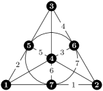
		$M=\left[\begin{smallmatrix}1&1&1&0&0&0&0\\ 1&0&0&1&1&0&0\\ 0&1&0&1&0&1&0\\ 0&0&1&0&1&1&0\\ 0&1&0&0&1&0&1\\ 0&0&1&1&0&0&1\\ 1&0&0&0&0&1&1\end{smallmatrix}\right]$
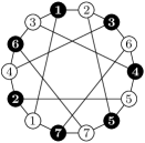
(i)		(ii)		(iii)

Figure 11.1. (i) The Fano plane. (ii) The incidence matrix $M$. (iii) The incidence graph of the Fano plane.

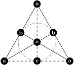
		$1234567$ $1234567$ $1234|56|7$ $16|2345|7$ $12|34|56|7$ $1|2345|6|7$ $(\mathcal{A}_{1},\mathcal{B}_{1})$ $(\mathcal{A}_{4},\mathcal{B}_{4})$ $(\mathcal{A}_{7},\mathcal{B}_{7})$ $123456|7$ $167|2345$ $1234|5|6|7$ $16|25|34|7$ $12|34|5|6|7$ $1|25|34|6|7$ $(\mathcal{A}_{2},\mathcal{B}_{2})$ $(\mathcal{A}_{5},\mathcal{B}_{5})$ $(\mathcal{A}_{8},\mathcal{B}_{8})$ $1234|567$ $123456|7$ $123|4|567$ $124|356|7$ $1|2|3|4|5|6|7$ $1|2|34|5|6|7$ $(\mathcal{A}_{3},\mathcal{B}_{3})$ $(\mathcal{A}_{6},\mathcal{B}_{6})$ $(\mathcal{A}_{9},\mathcal{B}_{9})$
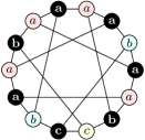
(i)		(ii)	(iii)

Figure 11.2. (i) The tactical decomposition $(\mathcal{A}_{4},\mathcal{B}_{4})$. (ii) Orbit representatives of the tactical decompositions of $M$. (iii) The tactical decomposition $(\mathcal{A}_{4},\mathcal{B}_{4})$ on the incidence graph.

The Fano plane is shown in Figure 11.1. The split and cir algorithm finds 100 tactical decompositions of the incidence matrix. Figure 11.2(ii) shows the orbit representatives. The self duality $\left(\begin{smallmatrix}1&2&3&4&5&6&7\\ 2&5&3&4&1&6&7\end{smallmatrix}\right)$ is visible as a horizontal reflection of the incidence graph. The two line notation means that each point in the first row is swapped with the corresponding line in the second row. This duality maps the tactical decomposition $(\mathcal{A}_{2},\mathcal{B}_{2})$ to $(\mathcal{A}_{3},\mathcal{B}_{3})$, maps $(\mathcal{A}_{5},\mathcal{B}_{5})$ to $(\mathcal{A}_{7},\mathcal{B}_{7})$, and maps $(\mathcal{A}_{i},\mathcal{B}_{i})$ to itself for $i\in\left\{1,4,8,9\right\}$. Finally, $(\mathcal{A}_{6},\mathcal{B}_{6})$ maps to itself by $\left(\begin{smallmatrix}1&2&3&4&5&6&7\\ 4&2&1&7&5&3&6\end{smallmatrix}\right)$. This self duality also acts as a reflection on the incidence graph.

For the tactical decomposition $(\mathcal{A}_{4},\mathcal{B}_{4})$, shown in Figure 11.2(i), the first duality maps points labeled $a$ to solid lines, points labeled $b$ to dashed lines, and the point labeled $c$ to the dotted line. This corresponds to the equitable partition of the incidence graph shown in Figure 11.2(iii).

References

- [1] Manuela A. D. Aguiar and Ana Paula S. Dias. The lattice of synchrony subspaces of a coupled cell network: characterization and computation algorithm. J. Nonlinear Sci., 24(6):949–996, 2014.
- [2] Manuela A. D. Aguiar and Ana Paula S. Dias. Synchronization and equitable partitions in weighted networks. Chaos, 28(7):073105, 8, 2018.
- [3] Manuela A. D. Aguiar, Ana Paula S. Dias, and Flora Ferreira. Patterns of synchrony for feed-forward and auto-regulation feed-forward neural networks. Chaos, 27(1):013103, 9, 2017.
- [4] Cesar O. Aguilar and Bahman Gharesifard. On almost equitable partitions and network controllability. American Control Conference (ACC), Boston, MA, pages 179–184, 2016.
- [5] Cesar O. Aguilar and Bahman Gharesifard. Almost equitable partitions and new necessary conditions for network controllability. Automatica J. IFAC, 80:25–31, 2017.
- [6] John W. Aldis. A polynomial time algorithm to determine maximal balanced equivalence relations. Internat. J. Bifur. Chaos Appl. Sci. Engrg., 18(2):407–427, 2008.
- [7] John William Aldis. On balance. PhD thesis, University of Warwick, 2010.
- [8] Oliver Bastert. Computing equitable partitions of graphs. Match, (40):265–272, 1999.
- [9] Igor Belykh and Martin Hasler. Mesoscale and clusters of synchrony in networks of bursting neurons. Chaos, 21(1):016106, 11, 2011.
- [10] Dieter Betten and Mathias Braun. A tactical decomposition for incidence structures. In Combinatorics ’90 (Gaeta, 1990), volume 52 of Ann. Discrete Math., pages 37–43. North-Holland, Amsterdam, 1992.
- [11] S. Bonaccorsi, S. Ottaviano, D. Mugnolo, and F. De Pellegrini. Epidemic outbreaks in networks with equitable or almost-equitable partitions. SIAM J. Appl. Math., 75(6):2421–2443, 2015.
- [12] Stanley Burris and H. P. Sankappanavar. A course in universal algebra, volume 78 of Graduate Texts in Mathematics. Springer-Verlag, New York-Berlin, 1981.
- [13] P. J. Cameron and R. A. Liebler. Tactical decompositions and orbits of projective groups. Linear Algebra Appl., 46:91–102, 1982.
- [14] Domingos M. Cardoso, Maria Aguieiras A. de Freitas, Enide Andrade Martins, and María Robbiano. Spectra of graphs obtained by a generalization of the join graph operation. Discrete Math., 313(5):733–741, 2013.
- [15] Domingos M. Cardoso, Charles Delorme, and Paula Rama. Laplacian eigenvectors and eigenvalues and almost equitable partitions. European J. Combin., 28(3):665–673, 2007.
- [16] Peter Dembowski. Verallgemeinerungen von Transitivitätsklassen endlicher projektiver Ebenen. Math. Z., 69:59–89, 1958.
- [17] Peter Dembowski. Finite geometries. Classics in Mathematics. Springer-Verlag, Berlin, 1997. Reprint of the 1968 original.
- [18] Magnus Egerstedt, Simone Martini, Ming Cao, Kanat Camlibel, and Antonio Bicchi. Interacting with networks: How does structure relate to controllability in single-leader, consensus networks? IEEE Control Systems Magazine, 32(4):66–73, 8 2012. Relation: https://www.rug.nl/research/jbi/ Rights: University of Groningen, Johann Bernoulli Institute for Mathematics and Computer Science.
- [19] Lucia Valentina Gambuzza and Mattia Frasca. A criterion for stability of cluster synchronization in networks with external equitable partitions. Automatica J. IFAC, 100:212–218, 2019.
- [20] A. Gerbaud. Spectra of generalized compositions of graphs and hierarchical networks. Discrete Math., 310(21):2824–2830, 2010.
- [21] David Gillis and Martin Golubitsky. Patterns in square arrays of coupled cells. J. Math. Anal. Appl., 208(2):487–509, 1997.
- [22] C. D. Godsil. Algebraic combinatorics. Chapman and Hall Mathematics Series. Chapman & Hall, New York, 1993.
- [23] C. D. Godsil. Equitable partitions. In Combinatorics, Paul Erdős is eighty, Vol. 1, Bolyai Soc. Math. Stud., pages 173–192. János Bolyai Math. Soc., Budapest, 1993.
- [24] I. Gohberg, P. Lancaster, and L. Rodman. Invariant subspaces of matrices with applications. Canadian Mathematical Society Series of Monographs and Advanced Texts. John Wiley & Sons, Inc., New York, 1986. A Wiley-Interscience Publication.
- [25] Martin Golubitsky, Ian Stewart, and Andrei Török. Patterns of synchrony in coupled cell networks with multiple arrows. SIAM J. Appl. Dyn. Syst., 4(1):78–100, 2005.
- [26] George Grätzer. Lattice theory: foundation. Birkhäuser/Springer Basel AG, Basel, 2011.
- [27] Hiroko Kamei and Peter J. A. Cock. Computation of balanced equivalence relations and their lattice for a coupled cell network. SIAM J. Appl. Dyn. Syst., 12(1):352–382, 2013.
- [28] Xianzhu Liu, Zhijian Ji, and Ting Hou. Graph partitions and the controllability of directed signed networks. Sci. China Inf. Sci., 62(4):042202, 11, 2019.
- [29] Yang-Yu Liu, Jean-Jacques Slotine, and Albert-Laszlo Barabasi. Controllability of complex networks. Nature, 473:167–73, 05 2011.
- [30] Simone Martini, Magnus Egerstedt, and Antonio Bicchi. Controllability decomposition of networked systems through quotient graphs. pages 5244–5249, 01 2008.
- [31] Brendan D. McKay. Backtrack Programming and the Graph Isomorphism Problem. Master’s thesis, Unversity of Melbourne, 1976.
- [32] Brendan D. McKay. Practical graph isomorphism. Numerical mathematics and computing, Proc. 10th Manitoba Conf., Winnipeg/Manitoba 1980, Congr. Numerantium 30, 45-87 (1981)., 1981.
- [33] Salvatore Monaco and Lorenzo Ricciardi Celsi. On multi-consensus and almost equitable graph partitions. Automatica J. IFAC, 103:53–61, 2019.
- [34] John M. Neuberger, Nándor Sieben, and James W. Swift. Computing eigenfunctions on the Koch snowflake: a new grid and symmetry. J. Comput. Appl. Math., 191(1):126–142, 2006.
- [35] John M. Neuberger, Nándor Sieben, and James W. Swift. Symmetry and automated branch following for a semilinear elliptic PDE on a fractal region. SIAM J. Appl. Dyn. Syst., 5(3):476–507 (electronic), 2006.
- [36] John M. Neuberger, Nándor Sieben, and James W. Swift. Automated bifurcation analysis for nonlinear elliptic partial difference equations on graphs. Internat. J. Bifur. Chaos Appl. Sci. Engrg., 19(8):2531–2556, 2009.
- [37] John M. Neuberger, Nándor Sieben, and James W. Swift. Newton’s method and symmetry for semilinear elliptic PDE on the cube. SIAM J. Appl. Dyn. Syst., 12(3):1237–1279, 2013.
- [38] John M. Neuberger, Nándor Sieben, and James W. Swift. Invariant Synchrony Subspaces of Sets of Matrices (companion web site), 2019. http://jan.ucc,nau.edu/ns46/invariant.
- [39] John M. Neuberger, Nándor Sieben, and James W. Swift. Synchrony and Antisynchrony for Difference-Coupled Vector Fields on Graph Network Systems. SIAM J. Appl. Dyn. Syst., 18(2):904–938, 2019.
- [40] Louis M. Pecora, Francesco Sorrentino, Aaron M. Hagerstrom, Thomas E. Murphy, and Rajarshi Roy. Cluster synchronization and isolated desynchronization in complex networks with symmetry. Nature Communications, 5(5079):1–8, 2014.
- [41] Amirreza Rahmani, Meng Ji, Mehran Mesbahi, and Magnus Egerstedt. Controllability of multi-agent systems from a graph-theoretic perspective. SIAM J. Control Optim., 48(1):162–186, 2009.
- [42] Aparna Rai, Priodyuti Pradhan, Jyothi Nagraj, Lohitesh Kovooru, Rajdeep Chowdhury, and Sarika Jalan. Understanding cancer complexome using networks, spectral graph theory and multilayer framework. Scientific Reports, 7:41676, 02 2017.
- [43] Michael T. Schaub, Neave O’Clery, Yazan N. Billeh, Jean-Charles Delvenne, Renaud Lambiotte, and Mauricio Barahona. Graph partitions and cluster synchronization in networks of oscillators. Chaos, 26(9):094821, 14, 2016.
- [44] Francesco Sorrentino, Louis M. Pecora, Aaron M. Hagerstrom, Thomas E. Murphy, and Rajarshi Roy. Complete characterization of the stability of cluster synchronization in complex dynamical networks. Sci. Adv., 2:1–8, 2016.
- [45] Ian Stewart. The lattice of balanced equivalence relations of a coupled cell network. Math. Proc. Cambridge Philos. Soc., 143(1):165–183, 2007.
- [46] Ian Stewart, Martin Golubitsky, and Marcus Pivato. Symmetry groupoids and patterns of synchrony in coupled cell networks. SIAM J. Appl. Dyn. Syst., 2(4):609–646, 2003.
- [47] The Sage Developers. SageMath, the Sage Mathematics Software System (Version 8.7), 2019. https://www.sagemath.org.
- [48] Shuo Zhang, M. Kanat Camlibel, and Ming Cao. Controllability of diffusively-coupled multi-agent systems with general and distance regular coupling topologies. In Proceedings of the 50th IEEE Conference on Decision and Control and European Control Conference (CDC-ECC), pages 759–764. University of Groningen, Research Institute of Technology and Management, 2011. Relation: https://www.rug.nl/fmns-research/itm/index Rights: University of Groningen, Research Institute of Technology and Management.
- [49] Shuo Zhang, Ming Cao, and M. Kanat Camlibel. Upper and lower bounds for controllable subspaces of networks of diffusively coupled agents. IEEE Trans. Automat. Control, 59(3):745–750, 2014.