Task Bench: A Parameterized Benchmark for Evaluating Parallel Runtime Performance

Abstract

We present Task Bench, a parameterized benchmark designed to explore the performance of distributed programming systems under a variety of application scenarios. Task Bench dramatically lowers the barrier to benchmarking and comparing multiple programming systems by making the implementation for a given system orthogonal to the benchmarks themselves: every benchmark constructed with Task Bench runs on every Task Bench implementation. Furthermore, Task Bench’s parameterization enables a wide variety of benchmark scenarios that distill the key characteristics of larger applications.

To assess the effectiveness and overheads of the tested systems, we introduce a novel metric, minimum effective task granularity (METG). We conduct a comprehensive study with 15 programming systems on up to 256 Haswell nodes of the Cori supercomputer. Running at scale, 100µs-long tasks are the finest granularity that any system runs efficiently with current technologies. We also study each system’s scalability, ability to hide communication and mitigate load imbalance.

I Introduction

The challenge of parallel and distributed computation has led to a wide variety of proposals for programming models, languages, and runtime systems. While these systems are well-represented in the literature, comprehensive and comparative performance evaluations remain difficult to find. Our goal in this paper is to develop a useful framework for comparing the performance of parallel and distributed programming systems, to help users and developers evaluate the performance tradeoffs of these systems.

Existing approaches to this problem focus on proxy-/mini-apps or microbenchmarks. These smaller codes distill key computational characteristics of larger applications: mini-apps are often derived from a larger code, and thus inherit some subset of its properties, while benchmarks are typically chosen to reflect a more narrow set of behavior(s). In either case, while a variety of insight can be gained, the overall programming effort required is proportional to the product of the number of systems and behaviors being evaluated. Few published studies compare more than a handful of systems [1, 2].

We present Task Bench, a parameterized benchmark for exploring the performance of parallel and distributed programming systems under a variety of conditions. The key property of Task Bench is that it completely separates the system-specific implementation from the implementation of the benchmarks themselves. In all previous benchmarks we know of, the effort to implement $m$ benchmarks on $n$ systems is $\mathcal{O}(mn)$. Task Bench’s design reduces this work to $\mathcal{O}(m+n)$, enabling dramatically more systems and benchmarks to be explored for the same amount of programming effort. New benchmarks created with Task Bench immediately run on all systems, and new systems that implement the Task Bench interface immediately run all benchmarks.

Benchmarks in Task Bench are based on the observation that regardless of the programming system in which an application is written, many applications can be modeled as coarse-grain units of work, called tasks, with dependencies between tasks representing the communication and synchronization required for parallel and distributed execution. By explicitly modeling the task graph (with tasks as vertices and dependencies as edges), we make it possible to explore a wide variety of patterns relevant to parallel and distributed computing: trivial parallelism, halo exchanges (as in structured and unstructured mesh codes), sweeps (as in the discrete ordinates method of simulating radiation), FFTs, trees (for divide and conquer), DNNs, graph analytics, etc. Tasks execute kernels with a variety of computational properties, including compute- and memory-bound loops of varying duration. Dependencies can be configured to carry communication payloads of varying size. Finally, multiple (potentially heterogeneous) task graphs can be executed concurrently to introduce task parallelism into the workload. Together, these elements enable the exploration of a large space of application behaviors—and make it easy to explore cases limited by runtime overhead as well as ones where computation or communication is dominant.

Adding a system to Task Bench involves implementing a set of standard services, such as executing a task or data transfer. Though benchmarks are described in terms of task graphs, this is simply a convenient representation of the computation, and the underlying system need not provide any native support for tasks. We provide Task Bench implementations in systems as diverse as MPI and Spark. Task Bench provides a core API that encapsulates functionality shared among systems, which reduces implementation effort and makes it much easier to achieve truly apples-to-apples comparisons between systems.

This approach has allowed us to benchmark 15 very different parallel and distributed programming systems (see Table 4). By running all systems on common benchmarks we were able to quantify phenomena that have never before been measured. Most strikingly, the overheads of systems we examine vary by more than five orders of magnitude, with popular, widely used systems at both ends of the spectrum! Clearly, slower systems have “good enough” performance for some applications, while presumably providing advantages in programmer productivity.

How does one predict whether performance will be good enough for a given application? The most commonly reported measures, weak and strong scaling, do not directly characterize the performance of the underlying programming system. Weak scaling can hide arbitrary amounts of runtime system overhead by using sufficiently large problem sizes, and strong scaling does not separate runtime system overhead from application costs (such as communication) that scale with the number of nodes when using progressively larger portions of a machine.

To characterize the contribution of runtime overheads to application performance, and as an example of the novel studies that can be done with Task Bench, we introduce a new metric called minimum effective task granularity (METG). Intuitively, for a given workload, METG(50%) is the smallest task granularity that maintains at least 50% efficiency, meaning that the application achieves at least 50% of the highest performance (in FLOP/s, B/s, or other application-specific measure) achieved on a given machine. The efficiency bound in METG is a key innovation over previous approaches, such as tasks per second (TPS), that fail to consider the amount of useful work performed (if tasks are non-empty [3, 4]) or to perform useful work at all (if tasks are empty [5]).

METG captures the important essence of a weak or strong scaling study, the behavior at the limit of scalability. For weak scaling, METG(50%) corresponds to the smallest problem size that can be weak-scaled with 50% efficiency. For strong scaling, METG(50%) can be used to compute the scale at which efficiency can be expected to dip below 50%. We note that METG(50%) for a given runtime system will vary with the application and the underlying hardware—i.e., METG(50%) is not a constant for a given system, but we find that systems have a characteristic range of METG(50%) values and that there is additional insight in the reasons that METG can vary.

A lower METG does not necessarily mean that performance for a particular workload is significantly better. Two systems with METG(50%) of 100 µs and 1 ms, respectively, running an application with 10 ms average task granularity, are both likely to perform well. Only when task granularity approaches (or drops below) METG(50%) will they likely diverge. METG identifies the regime in which a given system can deliver good performance, and explains how different systems coexist with runtime overheads that vary by orders of magnitude.

We conduct a comprehensive study of all 15 Task Bench implementations on up to 256 Haswell nodes of the Cori supercomputer [6]. Using METG, we find that a number of factors—node count, accelerators, and complex dependencies, among others—individually or in combination contribute to an order of magnitude or greater increase in METG, even in systems with the lowest overheads. While some systems can achieve sub-microsecond METG(50%) in best-case scenarios, we show that a more realistic bound for running nearly any application at scale is 100 µs with current technologies. Our study includes several asynchronous systems designed to provide benefits such as overlapped computation and communication. While small-scale benchmarks of these systems suffer from increased overhead, we find that the benefits of these systems become tangible at scale (provided the runtime overhead doesn’t increase beyond about 100 µs per task).

Beyond comparative study, the ability to explore a large configuration space also enables the discovery of bugs in the underlying systems. We found five performance issues, ranging from communication efficiency (Chapel, Realm), to the efficiency of task pruning, analysis and constant folding (PaRSEC, Dask and TensorFlow). Three have been fixed and all have been acknowledged by the developers of the respective systems. (All were either fixed or worked around in our experiments.) In some cases these correspond to order of magnitude or even asymptotic improvements in the performance of the underlying systems—benefits which apply well beyond Task Bench to all classes of applications. The bugs are described in more detail in Section VI.

The paper is organized as follows: Section II describes the Task Bench design. Section III discusses implementations in 15 systems. Section IV defines METG and its relationship to quantities of interest to application developers. Section V provides a comprehensive evaluation on Cori. Section VI describes bugs found with Task Bench. Section VII relates to previous efforts; Section VIII concludes.

II Task Bench

Parameter	Values	Purpose
height	height of graph	number of timesteps
width	width of graph	degree of parallelism
dependence	trivial, stencil, etc.	communication pattern
$\llcorner$ radix	(for nearest pattern)	dependencies per task
kernel	compute, memory, etc.	type of kernel
$\llcorner$ iter.	(for all kernels)	task duration
$\llcorner$ span	(for memory kernel)	bytes used per task per iter.
$\llcorner$ scratch	(for memory kernel)	total working set size
$\llcorner$ imbal.	(for load imbalance)	degree of imbalance
output	bytes per dependency	degree of comm.

Table 1: Task Bench parameters.

To explore as broad a space of application scenarios as possible, Task Bench provides a large number of configuration parameters. These parameters are described in Table 1, and control the size and structure of the task graph, the type and duration of kernels associated with each task, and the amount of data associated with each dependence edge in the graph.

Task graphs are a combination of an iteration space (with a task for each point in the space) with a dependence relation. For simplicity, but without loss of generality, the iteration space in Task Bench is constrained to be 2-dimensional, with time along the vertical axis and parallel tasks along the horizontal. Tasks may depend only on tasks from the immediately preceding time step. Figure 1 shows a number of sample task graphs that can be implemented with Task Bench. Note that layout is significant: generally speaking each column will be assigned to execute on a different processor core.

Dependencies between tasks are determined by a dependence relation. The dependence relation identifies the tasks from the previous time step each task depends on, permitting a wide variety of patterns to be implemented that are relevant to real applications: stencils, sweeps, FFTs, trees, etc. Dependence relations may be parameterized, such as picking the $K$ nearest neighbors, or $K$ distant neighbors. They may also vary over time, such as in the FFT pattern. The set of dependence relations is extensible, making it easy to add patterns to represent new classes of applications. Table 2 shows equations for the dependence relations of the patterns in Figure 1, where $t$ is timestep, $i$ is column, and $W$ is the width of the task graph.

(a) Trivial.

(b) Stencil.

(c) FFT.

(d) Sweep.

(e) Tree.

(f) Random.

Figure 1: Sample task graphs.

Pattern	Dependence Relation
Trivial	$D(t,i):=\emptyset$
Stencil	$D(t,i):=\{i,i-1,i+1\}$
FFT	$D(t,i):=\{i,i-2^{t},i+2^{t}\}$
Sweep	$D(t,i):=\{i,i-1\}$
Tree	$D(t,i):=\left\{\!\!\!\!\begin{array}[]{l l}\{i-2^{-t}W(i\operatorname{mod}2^{-t+1}W)\}&\text{if }t\leq\operatorname{log}_{2}W\\ \{i,i+2^{t-1}W^{-1}\}&\text{otherwise}\end{array}\right.\!\!\!\!$
Rand.	$D(t,i):=\{i|0\leq i<W\wedge\operatorname{random}()<0.5\}$

Table 2: Dependence relations for sample task graphs.

Listing 2 shows an excerpt from the Task Bench implementation in MPI. Methods of the Graph object g are provided by Task Bench’s core API and are shared among all implementations. These methods are summarized in Table 3. The MPI implementation follows the style of communicating sequential processes (CSP) [7], and executes a set of send and receive calls (lines 24 and 16, respectively) followed by executing the task body (line 32). Despite MPI having no notion of task, the execution of a task graph maps into the CSP style in a straightforward way. The implementation is both simple and efficient, but due to the choice of CSP makes no attempt to exploit task parallelism, and leaves performance on the table when executing task graphs with load imbalance or significant communication. Note the excerpt is simplified for presentation and the full implementation is more general and provides additional optimizations.

In addition to specifying the shape of the task graph, the core API also provides implementations of the kernels executed by each task as well as other utility routines (to parse inputs and display results). An excerpt from the core API compute kernel is shown in Listing 1. In addition to reducing the effort required to implement Task Bench, providing central implementations of these services ensures that all Task Bench implementations can be scripted uniformly and eliminates a potential source of performance disparity that can be a pitfall for other benchmarks.

The Task Bench core library is fully self-validating: The output of each task is a tuple $\langle\textrm{row, col}\rangle$ and is unique for a given task graph. Inputs are verified by checking the expected dependencies against those received, and an assertion is thrown if validation fails. These checks ensure that every execution of Task Bench is correct. Note that the graph representation is concise, making these checks very inexpensive. An evaluation of the performance impact of validation showed it to be less than 3% at the smallest task granularities in any Task Bench implementation, with a negligible effect on overall results.

Method	Purpose
Graph::contains_point(t,i)	is task(t,i) contained in the graph?
Graph::deps(t,i)	predecessors of task(t,i)
Graph::reverse_deps(t,i)	successors of task(t,i)
Graph::execute_point(t,i, …)	execute the body of task(t,i)

Table 3: Subset of the core API used in code samples below.

⬇

1void compute_kernel(long iterations) {

2 double A[64];

3 for (int i = 0; i < 64; i++) A[i] = 1.2345;

4 for (long iter = 0; iter < iterations; iter++)

5 for (int i = 0; i < 64; i++)

6 A[i] = A[i] * A[i] + A[i];

7}

Listing 1: Core API implementation of compute kernel.

⬇

1void execute_task_graph(Graph g) {

2 char *output = (char *)malloc(g.output_bytes);

3 char *scratch = (char *)malloc(g.scratch_bytes);

4 char **inputs = (char **)malloc(/*...*/);

5 long rank;

6 // initialize data structures...

7

8 std::vector<MPI_Request> requests;

9 for (long t = 0; t < g.height; ++t) {

10 if (g.contains_point(t, rank)) {

11 long idx = 0;

12 requests.clear();

13

14 for (long dep : g.deps(t, rank)) {

15 MPI_Request req;

16 MPI_Irecv(inputs[idx], g.output_bytes, MPI_BYTE,

17 dep, 0, MPI_COMM_WORLD, &req);

18 requests.push_back(req);

19 idx++;

20 }

21

22 for (long dep : g.reverse_deps(t, rank)) {

23 MPI_Request req;

24 MPI_Isend(output, g.output_bytes, MPI_BYTE,

25 dep, 0, MPI_COMM_WORLD, &req);

26 requests.push_back(req);

27 }

28

29 MPI_Waitall(requests.size(), requests.data(),

30 MPI_STATUSES_IGNORE);

31

32 g.execute_point(t, rank, output, inputs, scratch);

33 }

34 }

35}

Listing 2: Excerpt from Task Bench implementation in MPI.

Task Bench provides two main kernels that can be called from tasks: compute- and memory-bound. The compute-bound kernel executes a tight loop and is hand-written using AVX2 FMA intrinsics. The memory-bound kernel performs sequential reads and writes over an array, again with AVX2 intrinsics. The duration of both kernels can be configured by setting the number of iterations to execute; we use this ability to simulate the effects of varying application problem sizes. The memory-bound kernel is carefully written to keep the working set size constant as the number of iterations decreases, to avoid unwanted speedups due to cache effects.

III Implementations

We have implemented Task Bench in the 15 parallel and distributed programming systems listed in Table 4. These include traditional HPC programming models (MPI and MPI+X), PGAS and actor models (Chapel, Charm++ and X10), task-based systems (OmpSs, OpenMP 4.0, PaRSEC, Realm, Regent, and StarPU) and systems for large scale data analytics, machine learning and workflows (Dask, Spark, Swift/T, and TensorFlow). Implementing Task Bench in such a wide range of systems is possible because the separation between core API (in Table 3) and system implementation enables an overall effort of $\mathcal{O}(m+n)$ (for $m$ benchmarks on $n$ systems) rather than $\mathcal{O}(mn)$ as has been the case for all previous benchmarks that we know of. We briefly describe the systems and implementations below.

One challenge in targeting such a wide variety of systems is that the capabilities of the systems vary considerably. For example, some systems are implicitly parallel, and provide some form of parallelism discovery from sequential programs, whereas others are explicitly parallel and require users to specify the parallelism in the program. For systems that provide both implicit and explicit parallelism, the form of parallelism used in Task Bench is emphasized in Table 4.

In all cases, members of the programming systems’ teams were consulted in the development and evaluation of the corresponding Task Bench implementations. Where assistance was provided, the insights helped ensure that we provide the highest quality implementations for each system.

III-A Traditional HPC Programming Models

MPI [8] is a message-passing API for HPC. We provide an MPI implementation written in the style of communicating sequential processes (CSP). An excerpt is shown in Listing 2.

We provide two MPI+X implementations to evaluate hierarchical programming models. Our MPI+OpenMP implementation uses forall-style parallel loops to execute tasks, but otherwise follows the CSP implementation above. The code uses shared memory for data movement within a rank. Our MPI+CUDA implementation follows an offload model where data is copied to and from the GPU on every timestep.

III-B PGAS and Actor Models

PGAS and actor models, such as Chapel [9], Charm++ [10] and X10 [11] offer asynchronous tasks, making them amenable to a straightforward implementation of task bench. Synchronization is explicit and may be provided by messages (in actor models) or other primitives, such as locks or atomics (in PGAS models). PGAS models such as Chapel and X10 provide global references to data anywhere in the machine, but vary in whether data can be accessed remotely or not (Chapel allows this, X10 does not). Chapel also provides support for implicit parallelism which we do not evaluate in this paper.

III-C Task-Based Programming Models

Task-based systems include OmpSs [12], OpenMP 4.0 [13], PaRSEC [14, 15], Realm [16], Regent [17], and StarPU [18]. Though the details vary, these systems typically provide implicit parallelism, where tasks are enumerated sequentially (in program order) and the dependencies between tasks are analyzed automatically to construct a dependence graph that guides the execution of tasks. PaRSEC provides two modes, dynamic task discovery (DTD) [15], which operates as above, and parameterized task graphs (PTG) [14], where the dependence graph is constructed automatically from an analytical representation of the task graph. Realm (unlike the others above) is explicitly parallel and requires tasks to be connected explicitly via events. Realm is the low-level execution engine for Regent and thus serves as a limit study of what can be achieved with Regent. StarPU, in addition to its usual, implicitly parallel mode, also provides a mode where MPI is used for synchronization (and is thus explicitly parallel).

Among implicitly parallel, distributed task-based systems, there can be a scalability bottleneck due to enumerating tasks sequentially. PaRSEC and StarPU allow users to manually prune the task graph, skipping tasks not mapped for execution onto a given node, plus a “halo” consisting of tasks connected via dependencies to the set of node-local tasks. Because the dynamic checks to see if a task should be executed are not free of cost, we also provide versions of the PaRSEC and StarPU implementations (labeled shard and expl, respectively) hand-written to minimize such costs. PaRSEC shard uses the DTD mode but manually minimizes dynamic checks. StarPU expl uses the MPI integration described above. We see in Section V-D that such modifications are needed to achieve optimal scalability. Regent performs an equivalent optimization at compile time [19] that does not require user intervention and preserves the original, implicitly parallel programming model of the language.

System	Paradigm	Parallelism	Distrib.	Network
Chapel	multi-resolution	expl., impl.	yes	uGNI
Charm++	actor model	explicit	yes	uGNI
Dask	task-based	implicit	yes	sockets
MPI	message passing	explicit	yes	uGNI
MPI+X	hybrid	explicit	yes	MPI
OmpSs	loop-, task-based	expl., impl.	no
OpenMP	loop-, task-based	expl., impl.	no
PaRSEC	task-based	implicit	yes	MPI
Realm	task-based	explicit	yes	GASNet
Regent	task-based	implicit	yes	GASNet
Spark	functional	implicit	yes	sockets
StarPU	task-based	expl., impl.	yes	MPI
Swift/T	dataflow	implicit	yes	MPI
TensorFlow	dataflow	explicit	yes	sockets
X10	place-based	explicit	yes	MPI

Table 4: Systems for which we implemented Task Bench.

III-D Data Analytics, Machine Learning and Workflows

Dask [20], Spark [21] and TensorFlow [22] are programming models for large scale data analytics and machine learning. Dask and TensorFlow provide domain-specific abstractions built on top of task-based runtimes. Our implementations directly create tasks and are similar to other task-based systems above.

Spark provides support for functional operators that implicitly map to tasks. We use flatMap and groupByKey to generate dependencies and mapPartitions to execute tasks. An explicit hash partitioner ensures the correct task granularity.

Swift/T [23] is a parallel scripting language with dataflow semantics, used primarily for workflow automation. Our implementation is straightforward.

IV METG

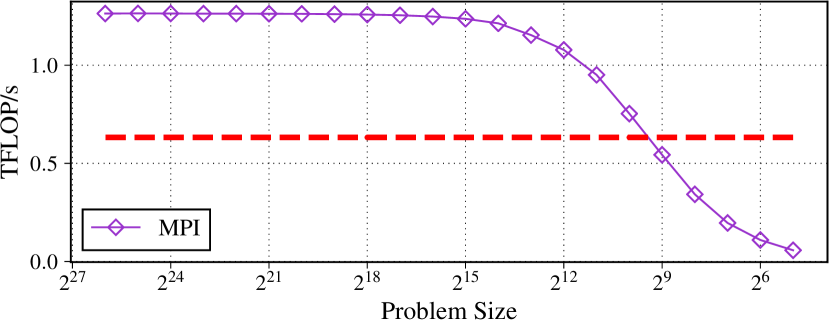
Figure 2: MPI FLOP/s vs problem size (stencil, 1 node).

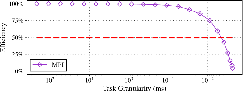
Figure 3: MPI efficiency vs task granularity (stencil, 1 node).

Since Task Bench permits rapid exploration of a large space of application scenarios, one question is how to characterize the performance and efficiency of systems under study. As noted above, the overheads of the systems we consider vary by more than five orders of magnitude, making it challenging to extract useful information from weak and strong scaling runs.

Existing studies of system efficiency typically report tasks per second (TPS). TPS results are difficult to interpret and apply, because efficiency (and thus the amount of useful work) is not constrained. With empty tasks [5], the resulting upper bound on task scheduling throughput fails to represent useful work within a realistic application. With non-empty tasks, since the efficiency of the overall application is typically not reported [3, 4], TPS is not a measurement of runtime-limited performance. Large tasks may be used to hide any amount of runtime overhead, while small tasks may result in a drop in total application throughput even as TPS increases.

We introduce minimum effective task granularity, or METG, an efficiency-constrained metric for runtime-limited performance. METG(50%) for an application $A$ is the smallest average task granularity (i.e., task duration) such that $A$ achieves overall efficiency of at least 50%. Note that METG is parameterized by the efficiency metric. For example, in compute-bound applications efficiency can be measured as the percentage of the available FLOP/s achieved. On Cori with 1.26 TFLOP/s available per Haswell node, METG(50%) corresponds to the smallest task granularity achieved while maintaining at least 0.63 TFLOP/s per node. However, METG is not tied to peak performance, and in applications not amenable to being characterized in this way, another application-specific measure of performance can be used. For example, a simulation on a mesh might use the number of mesh cells processed per second (i.e., total number of cells divided by wall clock time per iteration of the main simulation loop).

The choice of 50% is a parameter and not fundamental to METG. We use 50% in our studies to avoid pathologies associated with lower thresholds (see Section V-A), and also because it aligns with what we observe in practice. For example, one supercomputer center instructs users applying for projects to run a strong scaling study and then “select the most parallel efficient job size,” i.e., the largest number of nodes with a “ratio of benchmark speed-up vs. linear speed-up above 50%” [24], which corresponds to METG(50%).

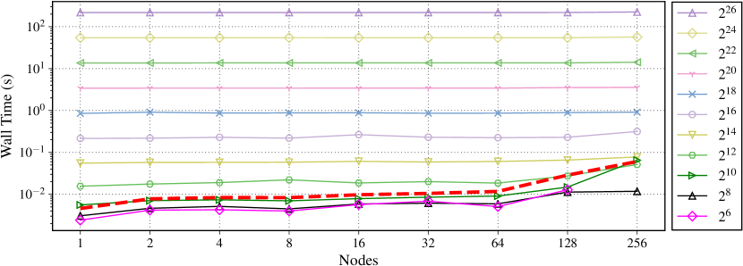
Figure 4: MPI weak scaling with problem size per node (stencil).

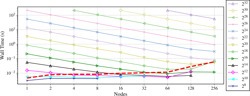
Figure 5: MPI strong scaling with problem size (stencil).

Figure 2 shows how METG is measured. We run the application (MPI Task Bench) on a Cori Haswell node with a problem size large enough that runtime is dominated by kernel execution. This result confirms that the application is properly configured and that the efficiency metric is achievable. The problem size is then repeatedly reduced while maintaining exactly the same hardware and software configuration (in particular, the same number of nodes and tasks). The expectation is that as problem size shrinks, performance will begin to drop and eventually approach zero. Systems with lower runtime overheads maintain higher performance at smaller problem sizes compared to systems with higher overheads.

To calculate METG, the data is replotted along axes of efficiency (i.e., as a percentage of the peak FLOP/s achieved) and task granularity (i.e., $\text{wall time}\times\text{num.~{}cores}/\text{num.~{}tasks}$), as shown in Figure 3. Note that a task is defined broadly to be any continuously-executing unit of application code, and thus it makes sense to discuss tasks even in systems with no explicit notion of tasking, such as MPI. In this case, the tasks run the compute-bound kernel shown in Section II.

In Figure 3, efficiency starts at 100%. Initially task granularity shrinks with minimal change in efficiency. As tasks shrink further, efficiency drops more rapidly, approaching a vertical asymptote as overhead comes to dominate useful work.

METG(50%) is the intersection of the curve at 50% efficiency, as shown by the red, dashed lines in Figures 2 and 3. At 50% efficiency, MPI achieves an average task granularity of 4.6 µs, thus the METG(50%) of MPI is 4.6 µs in this configuration.

METG has a well-defined relationship with quantities of interest such as weak and strong scaling. Figures 4 and 5 show the weak and strong scaling of MPI Task Bench running a stencil pattern at a variety of problem sizes. In these figures, the vertical axis is shown as wall time to emphasize the relationship to time-to-solution, but it could equivalently be shown as task granularity (as the number of tasks per execution is fixed). Intuitively, at larger problem sizes MPI is perfectly efficient. This can be seen at the top of each figure, with flat lines when weak scaling and ideally-sloped downward lines when strong scaling. Inefficiency begins to appear at smaller problem sizes, towards the bottom of the graph, where lines become more compressed. At the very bottom, the lines compress together as running time becomes dominated by overhead. Note that the contour of the bottom of each graph is identical and conforms to the METG curve (marked by the red, dashed line).

System	Version	Notes
Chapel	1.18.0	--fast
Charm++	6.9.0	-optimize
Dask	1.1.5
MPI(+X)	Cray MPICH 7.7.3	-O3
OmpSs	2, release 2020.06	-O3
OpenMP	Intel KMP 18.0.1.163	-O3
PaRSEC	Git master (242498d)	-O3
Realm	Git subgraph (5e9dcfa)	-O3
Regent	Git subgraph (5e9dcfa)	-fflow-spmd 1
Spark	2.3.0 (Scala 2.11.8, Java 8)
StarPU	1.3.4	-O3
Swift/T	1.4	-O3
TensorFlow	2.1.0
X10	Git master (9212dc2)	-O3 -NO_CHECKS

Table 5: System version and configuration notes.

METG therefore has a direct relationship with the smallest problem size that can be weak scaled to a given node count with a given level of efficiency. Using the formula for task granularity above, each run is 32 tasks wide and 1000 timesteps long, so task granularity is wall time divided by 1000 (since Cori has 32 cores per node). The $2^{12}$ problem size in Figure 4 scales well initially because the task granularity of 20 µs is greater than the METG(50%) of MPI at small node counts (which is about 4.6-12 µs from 1-64 nodes) but not at higher node counts (which rises to 28 µs at 128 nodes and 61 µs at 256). Similarly, METG corresponds to the point at which strong scaling can be expected to stop. In Figure 5 the problem size $2^{18}$ strong scales to 64 nodes, the point at which the scaling curve intersects METG(50%).

The METG metric has another useful property. Because METG is measured “in place” (i.e., without changing the number of nodes or cores available to the application), METG isolates effects due to shrinking problem size from effects due to increased communication and other resource issues as progressively larger portions of the machine are used.

V Evaluation

We present a comprehensive evaluation of our Task Bench implementations on up to 256 Haswell nodes of the Cori supercomputer [6], a Cray XC40 machine. Cori Haswell nodes have 2 sockets with Intel Xeon E5-2698 v3 processors (a total of 32 physical cores per node), 128 GB RAM, and a Cray Aries interconnect. We use GCC 7.3.0 for all Task Bench implementations, and (where applicable) the system default MPI implementation, Cray MPICH 7.7.3. Versions and flags for the various systems are shown in Table 5.

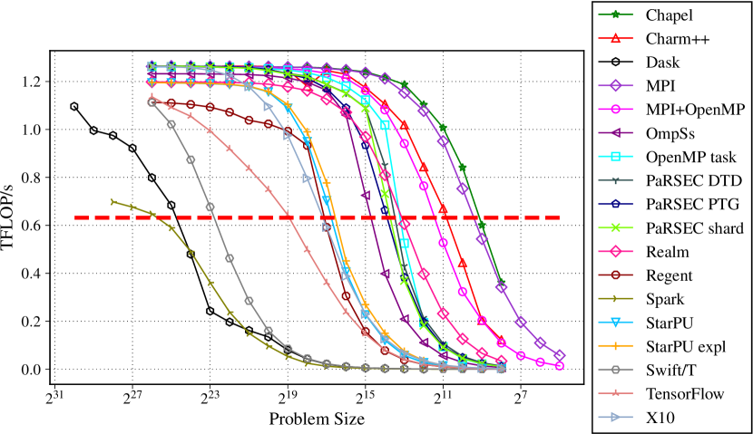
Figure 6: FLOPS vs problem size (stencil, 1 node). Higher is better.

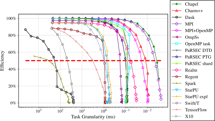
Figure 7: Efficiency vs task granularity (stencil, 1 node). Higher is better.

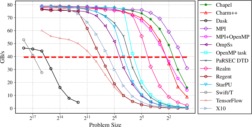
Figure 8: B/s vs problem size (stencil, 1 node). Higher is better.

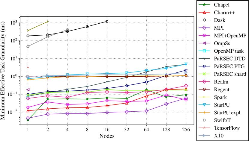
(a) Stencil pattern.

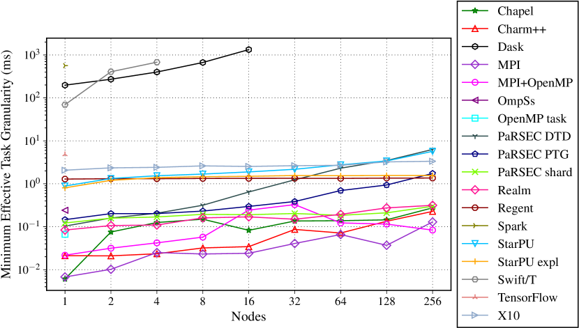
(b) Nearest pattern, 5 deps/task.

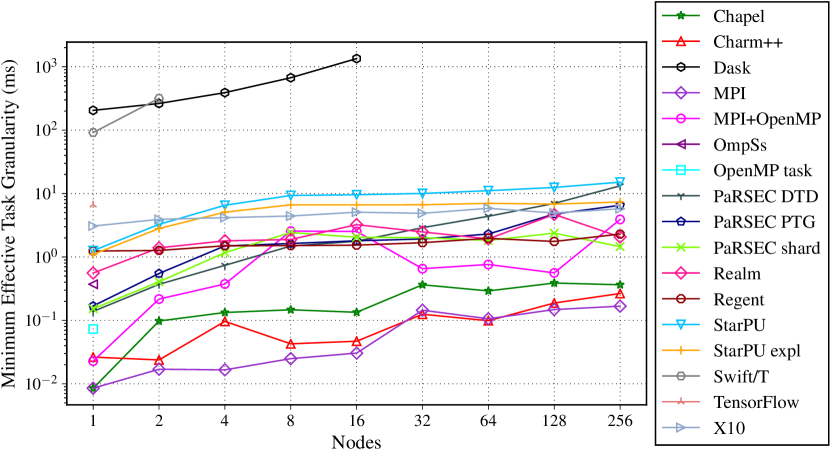
(c) Spread pattern, 5 deps/task.

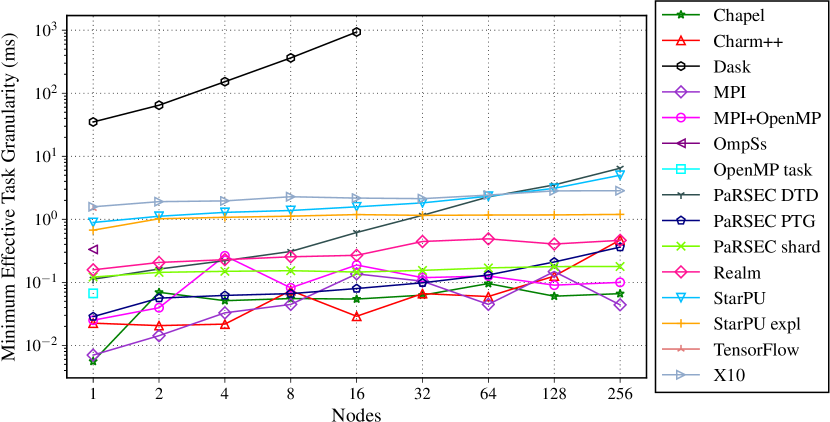
(d) Nearest pattern, 5 deps/task, 4 independent graphs.

Figure 9: METG vs node count for different dependence patterns. Lower is better.

For GPU experiments we use Piz Daint [25], a Cray XC50 with a Intel Xeon E5-2690 v3 (12 physical cores) and one NVIDIA Tesla P100 per node. We use GCC 6.2.0, Cray MPICH 7.7.2, and CUDA 9.1.85.

V-A Compute Kernel Performance

We first consider the peak performance achieved by each system. There should exist some task granularity which is sufficient to offset the runtime overheads of any system, regardless of how large those are. Even so, a variety of issues can lead to performance loss (e.g. due to not using all available cores). Verifying that peak performance is achieved ensures that there are no such flaws in our configuration.

Figure 6, which is the full version of Figure 2, shows the FLOP/s achieved with a compute-bound kernel with varying problem sizes (simulated by running the kernel for varying numbers of iterations). Each data point in the graph is a mean of 5 runs, with Task Bench configured to execute 1000 time steps of the stencil pattern. In the best case, we measure peak FLOP/s of $1.26\times 10^{12}$, which compares favorably with the officially reported number of $1.2\times 10^{12}$ [6]. We use our empirically determined number as the baseline for 100% efficiency below.

Most systems achieve or nearly achieve peak FLOP/s. Some systems reserve a number of cores (usually 1 or 2) for internal use (see below); these systems take a minor hit in peak FLOP/s compared to systems that share all cores between application and runtime. Some higher-overhead systems struggle to achieve peak FLOP/s, though in most cases the curves suggest that performance would continue to improve if we were to run larger problem sizes. Unfortunately, the excessive computational cost of running such tests makes this prohibitively expensive. For example, the Spark job in this case ran for over 6 hours.

Figure 7 plots efficiency (as a percentage of peak FLOP/s) vs. task granularity. As described in Section IV, this is used to calculate METG(50%). The red, dashed line indicates 50% efficiency. In most cases, task granularity asymptotes prior to this point, though some systems continue to improve at lower values. Accounting for this effect is one of the main arguments in favor of using reasonable efficiency thresholds for METG instead of empty tasks (i.e., METG(0%)). Empty tasks reward strategies, such as devoting 100% of system resources to the runtime system, that make no sense for real applications.

V-B Memory Kernel Performance

Figure 8 shows performance with a memory-bound kernel. We measure a peak memory bandwidth of 79 GB/s, using a working set size of 0.5 GB. As discussed in Section II, the kernels are designed to keep the working set constant as the number of iterations decrease to avoid noisy, superlinear effects in the results. For comparison, the OpenMP-enabled STREAM benchmarks [26] report up to 98 GB/s on the same hardware.

Not all cores are required to saturate memory bandwidth. This reduces the impact of reserving cores for system use (e.g. task-based systems that perform dependence analysis). Nearly all systems hit 100% of peak, unlike the compute-bound case.

The remaining experiments use compute-bound kernels.

V-C Baseline Overhead

One question when considering different programming systems is: How much overhead does the system add? This question is tricky to answer directly because some systems introduce overhead inline (i.e., by running system internal processes on the same cores as application tasks), while other systems introduce overhead out-of-line (i.e., by dedicating one or more cores solely to runtime use). Some systems, like Charm++, PaRSEC, Realm, and Regent, support both configurations.

To answer this question, we use METG as a proxy for overhead. Figure 9 shows how METG(50%) varies with node count for a subset of dependence patterns supported by Task Bench. METG(50%) is calculated separately at each node count, to distinguish runtime system behavior from changes in communication latency and topology when using progressively larger portions of the machine.

We consider the following configurations of Task Bench: Figure 9a is a 1D stencil where each task depends on 3 other tasks (including the same point in the previous timestep). Figure 9b is a pattern where each task depends on 5 others, chosen to be as close as possible. Figure 9c is a pattern where each task depends on 5 others, spread as widely as possible. And Figure 9d shows 4 identical copies of the nearest dependence pattern executing concurrently.

We observe that overheads vary by over 5 orders of magnitude. The most efficient systems are explicitly parallel and provide very lightweight mechanisms for parallelism. Task-based systems for HPC tend to be next most efficient, and provide additional features such as automatic dependency discovery and data movement. Higher overhead systems tend to be designed primarily for large-scale data analysis or workflows. It is worth remembering that these are minimum effective task granularities. Applications with an average task granularity of at least this value can usually be expected to execute efficiently. Typical task granularities will generally be determined by the application domain being considered. Most notably, for large-scale data analytics workloads, the higher METG values observed for Spark are sufficient. In contrast, for high-performance scientific simulations, task granularities in the millisecond range are useful, as such applications communicate (e.g., for halo exchanges) much more frequently.

The least complicated pattern (stencil) is most favorable to MPI, as it provides no opportunity for task parallelism. The dominating factor in this case is the overhead of executing a task, which is minimal for MPI as the code simply executes tasks in alternation with communication. The asynchrony of other systems is pure overhead in this scenario. MPI’s advantage shrinks as complexity grows, and even reverses as task parallelism is added in the form of multiple task graphs.

We omit Spark and Swift/T with more complicated dependencies, as their higher overheads require excessive problem sizes (beyond what completes in 6 hours) to reach 50% efficiency.

V-D Scalability

METG summarizes system overheads in a single number. This makes it possible to evaluate how communication topology and latency impact METG at different node counts, as shown in Figure 9. We find that systems with the smallest METG on one node have roughly an order of magnitude higher METG at 256 nodes. Increased communication latencies require significantly larger tasks to achieve the same level of efficiency, so apparent differences in overhead at small node counts can matter much less or not at all at larger node counts.

Most systems for HPC are highly scalable, but this is not true of all the systems included in this evaluation. Lower is better in Figure 9, and flat is ideal. Lines that rise with node count indicate less than ideal scaling. Most notably, Spark is primarily intended for industrial data center applications with task granularities measured in seconds. Spark uses a centralized controller, which limits throughput, and this is visible in the figure as the line for Spark immediately rises with node count. Keep in mind that Spark is being evaluated here with a nontrivial dependence pattern that is relatively unrepresentative of Spark’s normal use cases. Spark is more efficient with trivial parallelism, as described in Section V-E.

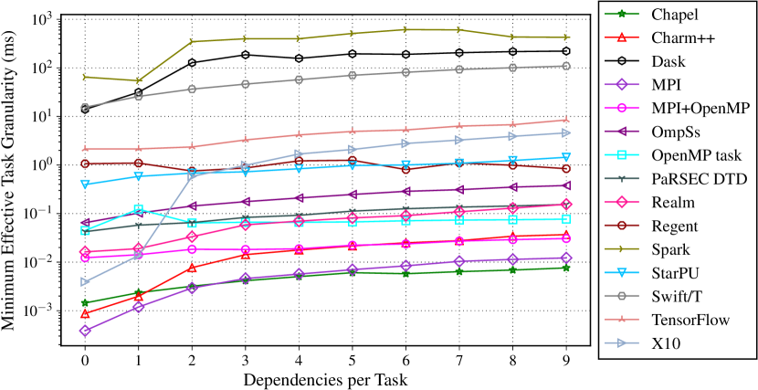
Figure 10: METG vs deps/task (nearest, 1 node). Lower is better.

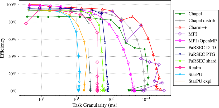
(a) 16 bytes per task dependency.

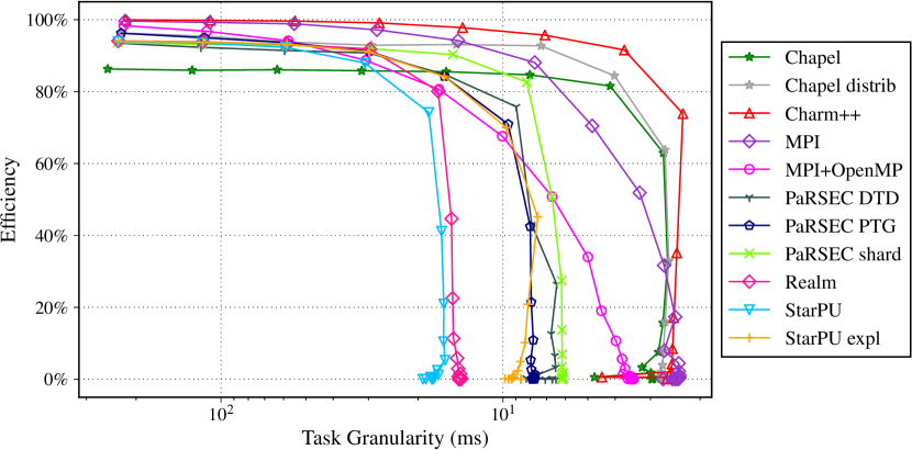
(b) 65536 bytes per task dependency.

Figure 11: Efficiency vs task granularity for varying communication (spread, 5 deps/task, 4 independent graphs, 64 nodes). Higher is better.

PaRSEC, StarPU and Regent rely on runtime analysis that can suffer from scalability bottlenecks if every node must consider the tasks executing on all other nodes. Although all three systems offer ways to improve scalability, these methods are not equally effective. PaRSEC DTD and StarPU allow users to manually prune tasks to reduce overhead; however the checks are not reduced to zero. Similarly, PaRSEC PTG uses compile-time optimizations to avoid the need for manual pruning, but still targets the PaRSEC DTD runtime and thus incurs some overhead. Figure 9 shows that these models do not provide ideal scalability, as seen by METG values that rise with increasing node count. Regent uses a compile-time optimization to generate code with a constant overhead per node [19]. Of the three systems, Regent is the only one that achieves ideal scalability while preserving its original, implicitly parallel programming model. The others can achieve ideal scalability but require increasing levels of manual intervention. PaRSEC shard includes additional manual optimizations over DTD to completely eliminate dynamic checks. StarPU expl is written in an explicitly parallel style using MPI for communication, and thus avoids any analysis bottleneck. These results indicate that the underlying systems are capable of scalable execution, but that the dynamic checks incurred by the implicitly parallel programming models hinder that scalability.

V-E Number of Dependencies

The number of dependencies per task has a strong influence on overhead, as shown in Figure 10. This plot shows METG(50%) for the nearest dependence pattern, when varying the number of dependencies per task from 0 to 9.

The ratio in METG between 0 and 3 dependencies per task ranges from $0.82\times$ to $250\times$ (mean $21\times$, std. dev. $64$). The large standard deviation shows that the sensitivity of system overhead to the dependency pattern varies widely. The largest ratios are among systems that perform runtime work inline. For example, MPI achieves an METG of 390 ns with 0 dependencies, but this rises to 4.6 µs with 3 dependencies, a $12\times$ increase. This is unsurprising, as with 0 dependencies no MPI_Isend calls are issued at all. Clearly, choosing a representative dependence pattern is important when estimating the performance of a workload or class of workloads.

V-F Overlapping Communication and Computation

Also of interest is the ability to hide communication latency in the presence of task parallelism. Figure 11 plots efficiency with varying amounts of communication, determined by the number of bytes produced by each task (and therefore communicated with each task dependency).

Asynchronous systems such as Charm++ demonstrate two benefits in these plots. First, by overlapping communication with computation, such systems execute smaller task granularities at higher levels of efficiency compared to the MPI implementations. Second, the asynchrony and scheduling flexibility from executing multiple graphs also makes the curves smoother, as spikes in latency due to interference from other jobs can be mitigated, leading to more predictable performance, especially at smaller message sizes.

The effectiveness of such overlap can be influenced by the scheduling policies of the underlying system. For example, Chapel’s default scheduler uses a round-robin policy; we see in Figure 11 that this approach fails to take full advantage of the available task parallelism. A work-stealing scheduler (Chapel distrib) is able to recover this performance.

V-G Load Imbalance

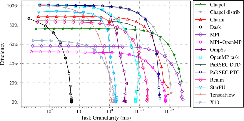
Figure 12: Efficiency vs task granularity under load imbalance (nearest pattern, 5 deps/task, 4 task graphs, 1 node). Higher is better.

One advantage of asynchronous execution is the ability to mitigate load imbalance with little or no additional programmer effort, especially in the presence of task parallelism. To quantify this effect, Figure 12 plots task granularity vs. efficiency under load imbalance where each task’s duration is multiplied by a uniform random variable in [0, 1). Task durations are generated with a deterministic pseudo random number generator with a consistent seed to ensure identical durations for all systems.

The MPI Task Bench, with its distinct computation and communication phases, suffers the most under load imbalance. The biggest difference is at large task granularities, where the imbalance effectively puts an upper bound on efficiency. At smaller task granularities the effect shrinks and may even reverse as systems hit their fundamental limits due to overhead.

The remaining differences are due primarily to different scheduling behaviors. The execution of 4 simultaneous task graphs only partially mitigates the load imbalance between tasks. Systems that provide an additional on-node work stealing capability (such as Chapel with the distrib scheduler) see additional gains in efficiency at large task granularities. However, the use of work-stealing queues can also impact throughput at small task granularities. For example, Chapel’s default (non-work-stealing) scheduler outperforms distrib at very small task granularities. We do not consider Charm++ load balancers because the imbalance is non-persistent (i.e., timestep $t$ is uncorrelated with timestep $t+1$). We leave analysis of persistent load imbalance to future work.

V-H Heterogeneous Processors

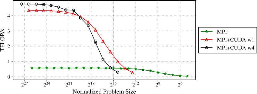
Figure 13: GPU FLOP/s vs normalized problem size (stencil, 1 node). Higher is better.

To determine the cost of scheduling tasks on GPUs, Figure 13 compares MPI and MPI+CUDA on Piz Daint [25]. The CUDA compute kernel achieves $4.759\times 10^{12}$ FLOP/s, which is very close to the officially reported number $4.761\times 10^{12}$. The CPU achieves $5.726\times 10^{11}$ FLOP/s. Note that the kernels perform different numbers of operations as the GPU requires more work to reach peak performance. The x-axis in Figure 13 is normalized to keep FLOPs constant for a given problem size.

Our MPI+CUDA code uses an offload model with data copied to/from the GPU every step. In our tests, w1 uses 1 task per GPU, whereas w4 overdecomposes, using 4 MPI ranks per GPU to push work to the GPU in parallel. w4 achieves higher FLOP/s but drops more rapidly at small problem sizes, due to the overhead of running $4\times$ as many CUDA kernels. Either way, GPUs require more work to achieve high performance, and the overhead of copying data dominates at small task granularities, where CPUs achieve higher performance. While Figure 13 is not couched in terms of METG (as peak performance on CPU and GPU are very different), the conclusion here is similar to Section V-D: the cost of sending data and tasks to GPUs imposes a floor on task granularity relative to CPUs, reducing the advantage at small task granularities of very lightweight mechanisms such as those in MPI.

V-I Validating METG with Time to Solution

We can use METG to predict the scalability of a code. Figure 14 shows strong scaling for three Task Bench implementations with the stencil pattern. Lines marked “actual” represent strong scaling measurements, while ones marked “limit 50%” are computed by multiplying METG(50%) by tasks per core (in this case, 1000) to obtain wall clock time. Intuitively, “limit” is the smallest time to solution that can be achieved for any problem size at that node count, while maintaining 50% efficiency. Data points where “actual” falls below “limit” mark points where strong scaling parallel efficiency is less than 50%.

There are two points of interest on each “limit 50%” curve: the point where it intersects “actual” and the point where it intersects an ideal scaling curve, computed by taking the initial time to solution and assuming linear scaling. These points are marked for Charm++ in Figure 14 with a black square and black circle, respectively. Notably, the ideal-limit intersection (black circle) requires only a run of the application on one node, combined with METG(50%) measurements, to estimate the strong scalability of the code: i.e., the smallest time to solution, and the number of nodes at which that time is achieved, while maintaining at least 50% efficiency. In Figure 14, the error in the estimate is the distance between the black square and circle; these are separated by a factor of $1.22\times$ in node count, and $1.27\times$ in time to solution.

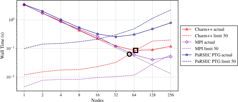
Figure 14: Strong scaling vs efficiency-limited time to solution with problem size $2^{20}$ (stencil). Lower is better.

	Nodes		Time to Solution
Pattern	mean	std. dev.	mean	std. dev.
stencil	$1.64\times$	0.278	$1.26\times$	0.246
nearest	$1.75\times$	0.268	$1.15\times$	0.331
spread	$1.43\times$	0.288	$1.29\times$	0.206
nearest, 4 graphs	$1.96\times$	0.680	$1.26\times$	0.702

Table 6: Factor of separation between limit-ideal and limit-actual intersections across all 12 programming systems tested in Section V-D.

Table 6 expands this comparison to the 4 patterns tested in Section V-D for all 12 programming systems that scale well enough to evaluate the separation between the limit-ideal and limit-actual intersections. We see that overall, the mean separation is at most $1.96\times$ in node count and at most $1.29\times$ in time to solution, making this a useful way to predict strong scaling in the 4 patterns we tested in Section V-D.

VI Performance Issues Discovered

Task Bench is useful not only as a tool for evaluating programming system performance, but also for discovering potential areas for improvement. During the development of Task Bench, we identified a number of performance issues in the underlying programming systems. These discoveries were possible because of the flexibility of Task Bench, and our ability to rapidly run new experiments with a variety of application scenarios. All issues were reported to and acknowledged by the respective system’s developers, and are either fixed or worked around in our experiments. We describe them below.

Realm and Chapel both use DMA subsystems optimized for large copies. Early Task Bench experiments revealed high METG values, diagnosed by the Realm/Chapel developers as overhead due to the cost of scheduling small copies. Subsequent improvements in Realm and Chapel improved small copy overheads (and thus METG) by over an order of magnitude in the case of Realm, and by $2\times$ in the case of Chapel. These improvements affect any application where fine-grained data movement is needed, which is particularly relevant in strong scaling regimes when running on large numbers of nodes.

Further analysis of Realm efficiency indicated many overheads due to dynamic graph construction. The Realm developers implemented a new “subgraph” API in response to this feedback to amortize the cost of repeatedly constructing isomorphic task graphs. This API is used in Task Bench to achieve further speedups in the Realm implementation.

Chapel uses a naive round-robin scheduler by default, which can lead to unexpected load balance issues because certain language features (such as remote array assignment) implicitly generate tasks. This resulted in poor peak performance, even at large task granularities, which in some cases made it impossible to measure METG (because peak efficiency did not exceed 50%). Chapel’s other schedulers add overhead, resulting in higher METGs. Based on guidance from the Chapel team, we worked around this with a serial block.

PaRSEC uses task pruning to reduce analysis work performed on each node, and thus improve scalability at large node counts. Initial Task Bench results achieved less than the expected scalability: METG was rising too quickly with node count. The PaRSEC developers diagnosed a bug in task pruning—the optimization was failing to trigger—and it was subsequently fixed. We also implemented a version of the PaRSEC code, shard, which uses manual pruning to demonstrate that additional gains may still be possible.

Early Task Bench results for Dask revealed that the cost of scheduling a task was $\mathcal{O}(N)$ where $N$ is the number of tasks in a task graph, causing overall cost for a task graph with $N$ nodes to be $\mathcal{O}(N^{2})$. This issue was reported to and confirmed by the Dask developers; the bug is suspected to be in optimizations performed on the task graph by Dask. As a workaround, our results in the paper use a lower-level interface which does not suffer from this asymptotic slowdown.

TensorFlow performs optimizations on task graphs prior to execution, including a constant folding pass. The Task Bench implementation uses aggressive loop unrolling to minimize overheads, resulting in the task graph being marked as constant. Because TensorFlow optimizations are performed on a single core, this resulted in sequential execution of the entire graph, and Task Bench experiments timed out. As a workaround, additional inputs are fed to nodes in the graph to make them non-constant, forcing them to be executed by TensorFlow’s parallel scheduler. Though this was exacerbated by Task Bench’s approach to unrolling loops, it affects any task graph with constants that are expensive to compute where the users may wish to perform constant-folding in parallel.

In all cases, we found bugs that are applicable outside of Task Bench and that impact metrics other than METG. Notably, the scalability issues and asymptotic complexity have a growing impact with larger node counts and will eventually become visible with nearly any application. In other cases, Task Bench and METG made it possible to identify performance degradation at the extremes of application configurations which might remain hidden with full-size applications, particularly when evaluated with weak and strong scaling alone. The improvements motivated by our findings are nonetheless relevant in strong-scaling regimes in a variety of applications, particularly as node and core counts grow.

VII Related Work

Parallel and distributed programming systems are often evaluated using proxy- or mini-apps, or microbenchmarks. Mini-apps are explicitly derived from larger applications and hence have the advantage of bearing some relationship to the original. This advantage typically does not hold for microbenchmarks.

Though smaller than full applications, mini-apps can be challenging to implement to a level of quality sufficient for conducting comparative studies between programming systems. The largest studies we know of consider at most 7 and 6 programming systems, respectively [1, 2], and the latter only considers on-node programming models. In both cases, the mini-apps under study require a separate, tuned implementation (in contrast to Task Bench). Other studies usually lack a comprehensive evaluation, even if multiple implementations are available:

• The PENNANT reference implementation supports MPI/OpenMP/MPI+OpenMP [27]. A follow-up paper presents a Regent implementation [17].

• One follow-up paper for the mini-app CoMD describes a Chapel implementation [28] (comparison against reference only). Additional follow-up papers consider aspects of the reference implementation only [29, 30].

• A report on the Mantevo project [31] describes a number of mini-apps, but only includes self-comparisons based on reference implementations.

• A report on MiniAero [32] describes four implementations of the mini-app, but only includes performance results for three, of which only two can be compared in an apples-to-apples manner as the last implementation uses structured rather than unstructured meshes. A follow-up describes another implementation in Regent [17] (comparison vs. reference only).

Microbenchmarks can be easier to implement, but do not address the asymptotic costs of implementation. PRK Stencil [33] contains a 2D stencil and is evaluated on implementations in MPI, SHMEM, UPC, Charm++, and Grappa [34]. The NAS benchmark suite [35, 36] consists mostly of small kernels for dense or sparse matrix computations and has implementations in OpenMP [37], MPI and MPI+OpenMP [38], and Charm++ [39]. PRK requires $\mathcal{O}(n)$ effort to implement (for $n$ systems) by virtue of being only a single computational pattern, while NAS requires $\mathcal{O}(mn)$ overall effort (for $m$ patterns and $n$ systems). In contrast, Task Bench requires $\mathcal{O}(m+n)$ effort and is easily extended to cover new systems or patterns with $\mathcal{O}(1)$ effort for each additional system or pattern.

System-specific benchmarks quantify specific aspects of system performance, such as MPI communication or collective latency [40, 41]. These measurements typically do not generalize beyond the immediate system they measure.

coNCePTuaL [42] is a domain-specific language for writing network performance tests. coNCePTuaL and Task Bench both enable the easy creation of new benchmarks, though coNCePTuaL does so via scripting whereas Task Bench provides a set of configurable parameters. coNCePTuaL also targets a lower level of abstraction, optimized more for testing messaging layers, whereas Task Bench is closer to application level and therefore enables comparisons of a broader set of parallel and distributed programming systems.

Limit studies of task scheduling throughput in various runtime systems often make additional assumptions. A popular assumption is the use of trivially parallel tasks [3, 4], which as shown in Section V-E underestimates (often substantially) the cost of scheduling a task and can also impact scalability.

VIII Conclusion

Task Bench is a new approach for evaluating the performance of parallel and distributed programming systems. By separating the specification of a benchmark from implementations in various programming systems, Task Bench reduces overall developer effort to $\mathcal{O}(m+n)$ (for $m$ benchmarks on $n$ systems) rather than $\mathcal{O}(mn)$ as has been the case for all previous benchmarks that we know of. This has enabled us to explore a broad space of application scenarios and to do so with a large number of programming systems. Our experiments have enabled the following insights:

• Evaluations of programming system performance should avoid using TPS, or strong or weak scaling to characterize overheads, as these metrics do not constrain the useful work achieved. Instead a metric with constrained efficiency, such as METG(50%), is needed to ensure that measurements are representative and fair.

• METG for current distributed programming systems varies by over 5 orders of magnitude. Clearly understanding the needed task granularity is an important consideration in choosing a programming system for a new application.

• While some systems support METG(50%) as small as 390 ns, this applies only to trivial dependencies and small CPU-based clusters. A number of factors (nontrivial dependencies, accelerators and cluster sizes in the hundreds of nodes) raise the METGs that can be achieved by over an order of magnitude: 100 µs is a reasonable bound for most applications running at scale with current technologies.

• Systems that support asynchronous execution show benefits under balanced computation and communication, and load imbalance. However, these gains can be nullified by high baseline overheads.

• Task-based systems that rely on runtime analysis for the discovery of parallelism can suffer from sequential bottlenecks that limit scaling. Existing, dynamic task pruning techniques are not sufficient to fully mitigate this bottleneck, while static, compile-time approaches are able to do so.

• Systems for large scale data analysis require very large tasks (tens of seconds) to scale beyond small node counts, reflecting the very coarse tasks and lack of need for strong scaling in current workloads.

• Task Bench has proven effective in finding performance issues and has lead to substantial improvements in several systems we study.

Not considered in our analysis is the impact of programming system features on programmer productivity and performance portability. Most applications do not operate at the absolute extreme of runtime-limited performance, and thus may choose to trade overhead for usability. Our study helps to quantify the performance side of that tradeoff so that users can be better informed and developers can see the impact that features have on the performance of their programming systems.

References

- [1] I. Karlin, A. Bhatele, J. Keasler, B. L. Chamberlain, J. Cohen, Z. Devito, R. Haque, D. Laney, E. Luke, F. Wang, D. Richards, M. Schulz, and C. H. Still, “Exploring traditional and emerging parallel programming models using a proxy application,” in International Parallel and Distributed Processing Symposium (IPDPS). IEEE, 2013.
- [2] T. Deakin, S. McIntosh-Smith, J. Price, A. Poenaru, P. Atkinson, C. Popa, and J. Salmon, “Performance portability across diverse computer architectures,” in Workshop on Performance, Portability and Productivity in HPC (P3HPC). IEEE, 2019, pp. 1–13.
- [3] H. Qu, O. Mashayekhi, D. Terei, and P. Levis, “Canary: A scheduling architecture for high performance cloud computing,” CoRR, vol. abs/1602.01412, 2016. [Online]. Available: http://arxiv.org/abs/1602.01412
- [4] T. G. Armstrong, J. M. Wozniak, M. Wilde, and I. T. Foster, “Compiler techniques for massively scalable implicit task parallelism,” in Supercomputing (SC), 2014.
- [5] W. Lee, E. Slaughter, M. Bauer, S. Treichler, T. Warszawski, M. Garland, and A. Aiken, “Dynamic Tracing: Memoization of task graphs for dynamic task-based runtimes,” in Supercomputing (SC), 2018.
- [6] “Cori Configuration,” https://www.nersc.gov/users/computational-systems/cori/configuration/, 2015.
- [7] C. A. R. Hoare, “Communicating sequential processes,” Communications of the ACM, vol. 21, no. 8, pp. 666–677, 1978.
- [8] M. Snir, S. Otto, S. Huss-Lederman, D. Walker, and J. Dongarra, MPI-The Complete Reference. MIT Press, 1998.
- [9] B. L. Chamberlain, “Chapel,” in Programming Models for Parallel Computing, P. Balaji, Ed. MIT Press, 2015, pp. 129–159.
- [10] L. V. Kalé and S. Krishnan, “CHARM++: A portable concurrent object oriented system based on C++,” in OOPSLA, 1993, pp. 91–108.
- [11] P. Charles, C. Grothoff, V. Saraswat, C. Donawa, A. Kielstra, K. Ebcioglu, C. Von Praun, and V. Sarkar, “X10: An object-oriented approach to non-uniform cluster computing,” in OOPSLA, 2005.
- [12] A. Duran, E. Ayguadé, R. M. Badia, J. Labarta, L. Martinell, X. Martorell, and J. Planas, “OmpSs: A proposal for programming heterogeneous multi-core architectures,” Parallel Processing Letters, vol. 21, no. 02, pp. 173–193, 2011.
- [13] “OpenMP application program interface,” http://www.openmp.org/wp-content/uploads/OpenMP4.0.0.pdf, 2013.
- [14] G. Bosilca, A. Bouteiller, A. Danalis, M. Faverge, T. Hérault, and J. J. Dongarra, “PaRSEC: Exploiting heterogeneity to enhance scalability,” Computing in Science & Engineering, vol. 15, no. 6, pp. 36–45, 2013.
- [15] R. Hoque, T. Herault, G. Bosilca, and J. Dongarra, “Dynamic task discovery in PaRSEC: A data-flow task-based runtime,” in Proceedings of the 8th Workshop on Latest Advances in Scalable Algorithms for Large-Scale Systems, ser. ScalA ’17. New York, NY, USA: ACM, 2017, pp. 6:1–6:8. [Online]. Available: http://doi.acm.org/10.1145/3148226.3148233
- [16] S. Treichler, M. Bauer, and A. Aiken, “Realm: An event-based low-level runtime for distributed memory architectures,” in Parallel Architectures and Compilation Techniques (PACT), 2014.
- [17] E. Slaughter, W. Lee, S. Treichler, M. Bauer, and A. Aiken, “Regent: A high-productivity programming language for HPC with logical regions,” in Supercomputing (SC), 2015.
- [18] C. Augonnet, S. Thibault, R. Namyst, and P.-A. Wacrenier, “StarPU: A unified platform for task scheduling on heterogeneous multicore architectures,” Concurrency and Computation: Practice and Experience, vol. 23, pp. 187–198, Feb. 2011.
- [19] E. Slaughter, W. Lee, S. Treichler, W. Zhang, M. Bauer, G. Shipman, P. McCormick, and A. Aiken, “Control Replication: Compiling implicit parallelism to efficient SPMD with logical regions,” in Supercomputing (SC), 2017.
- [20] M. Rocklin, “Dask: Parallel computation with blocked algorithms and task scheduling,” in Python in Science Conference (SciPy), no. 130-136. Citeseer, 2015.
- [21] M. Zaharia, M. Chowdhury, M. J. Franklin, S. Shenker, and I. Stoica, “Spark: Cluster computing with working sets,” HotCloud, vol. 10, pp. 10–10, 2010.
- [22] M. Abadi, A. Agarwal, P. Barham, E. Brevdo, Z. Chen, C. Citro, G. S. Corrado, A. Davis, J. Dean, M. Devin, S. Ghemawat, I. Goodfellow, A. Harp, G. Irving, M. Isard, Y. Jia, R. Jozefowicz, L. Kaiser, M. Kudlur, J. Levenberg, D. Mané, R. Monga, S. Moore, D. Murray, C. Olah, M. Schuster, J. Shlens, B. Steiner, I. Sutskever, K. Talwar, P. Tucker, V. Vanhoucke, V. Vasudevan, F. Viégas, O. Vinyals, P. Warden, M. Wattenberg, M. Wicke, Y. Yu, and X. Zheng, “TensorFlow: Large-scale machine learning on heterogeneous systems,” http://tensorflow.org/, 2015.
- [23] J. M. Wozniak, T. G. Armstrong, M. Wilde, D. S. Katz, E. Lusk, and I. T. Foster, “Swift/T: Large-scale application composition via distributed-memory dataflow processing,” in Cluster, Cloud and Grid Computing (CCGrid), 2013.
- [24] “Technical Report - CSCS,” https://user.cscs.ch/access/report, 2019.
- [25] “Piz Daint - CSCS,” http://www.cscs.ch/computers/piz_daint, 2016.
- [26] J. D. McCalpin, “STREAM benchmark,” https://www.cs.virginia.edu/stream/, 1995.
- [27] C. R. Ferenbaugh, “PENNANT: an unstructured mesh mini-app for advanced architecture research,” Concurrency and Computation: Practice and Experience, 2014.
- [28] R. Haque and D. Richards, “Optimizing PGAS overhead in a multi-locale Chapel implementation of CoMD,” in PGAS Applications Workshop (PAW). IEEE, 2016, pp. 25–32.
- [29] O. Pearce, H. Ahmed, R. W. Larsen, P. Pirkelbauer, and D. F. Richards, “Exploring dynamic load imbalance solutions with the comd proxy application,” Future Generation Computer Systems, 2017.
- [30] P. Cicotti, S. M. Mniszewski, and L. Carrington, “An evaluation of threaded models for a classical md proxy application,” in Workshop on Hardware-Software Co-Design for High Performance Computing. IEEE Press, 2014, pp. 41–48.
- [31] M. A. Heroux, D. W. Doerfler, P. S. Crozier, J. M. Willenbring, H. C. Edwards, A. Williams, M. Rajan, E. R. Keiter, H. K. Thornquist, and R. W. Numrich, “Improving Performance via Mini-applications,” Sandia National Laboratories, Tech. Rep. SAND2009-5574, 2009.
- [32] J. Bennett, R. Clay, G. Baker, M. Gamell, D. Hollman, S. Knight, H. Kolla, G. Sjaardema, N. Slattengren, K. Teranishi, J. Wilke, M. Bettencourt, S. Bova, K. Franko, P. Lin, R. Grant, S. Hammond, S. Olivier, L. Kale, N. Jain, E. Mikida, A. Aiken, M. Bauer, W. Lee, E. Slaughter, S. Treichler, M. Berzins, T. Harman, A. Humphrey, J. Schmidt, D. Sunderland, P. McCormick, S. Gutierrez, M. Schulz, A. Bhatele, D. Boehme, P.-T. Bremer, and T. Gamblin, “ASC ATDM Level 2 milestone #5325: Asynchronous many-task runtime system analysis and assessment for next generation platforms,” no. SAND2015-8312, 2015.
- [33] R. F. Van der Wijngaart and T. G. Mattson, “The parallel research kernels,” in HPEC, 2014, pp. 1–6.
- [34] R. F. Van der Wijngaart, A. Kayi, J. R. Hammond, G. Jost, T. S. John, S. Sridharan, T. G. Mattson, J. Abercrombie, and J. Nelson, “Comparing runtime systems with exascale ambitions using the parallel research kernels,” in International Conference on High Performance Computing. Springer, 2016, pp. 321–339.
- [35] D. H. Bailey, E. Barszcz, J. T. Barton, D. S. Browning, R. L. Carter, L. Dagum, R. A. Fatoohi, P. O. Frederickson, T. A. Lasinski, R. S. Schreiber, and H. D. Simon, “The NAS parallel benchmarks summary and preliminary results,” in Supercomputing (SC), 1991.
- [36] D. Bailey, T. Harris, W. Saphir, R. Van Der Wijngaart, A. Woo, and M. Yarrow, “The NAS parallel benchmarks 2.0,” Technical Report NAS-95-020, NASA Ames Research Center, Tech. Rep., 1995.
- [37] H.-Q. Jin, M. Frumkin, and J. Yan, “The OpenMP implementation of NAS parallel benchmarks and its performance,” 1999.
- [38] F. Cappello and D. Etiemble, “MPI versus MPI+OpenMP on IBM SP for the NAS benchmarks,” in Supercomputing (SC), 2000, p. 12.
- [39] S. Krishnan, M. Bhandarkar, and L. V. Kalé, “Object-oriented implementation of the NAS parallel benchmarks using Charm++,” 1996.
- [40] W. Gropp and E. L. Lusk, “Reproducible measurements of MPI performance characteristics,” in Recent Advances in Parallel Virtual Machine and Message Passing Interface, 6th European PVM/MPI Users’ Group Meeting, 1999, pp. 11–18.
- [41] D. Grove, P. Coddington et al., “Precise MPI performance measurement using mpibench,” in Proceedings of HPC Asia. Citeseer, 2001, pp. 24–28.
- [42] S. Pakin, “The design and implementation of a domain-specific language for network performance testing,” IEEE Transactions on Parallel and Distributed Systems, vol. 18, no. 10, pp. 1436–1449, 2007.