The impact of the observed baryon distribution in haloes on the total matter power spectrum

Abstract

The interpretation of upcoming weak gravitational lensing surveys depends critically on our understanding of the matter power spectrum on scales $k<$10\text{\,}$\mathrm{\mathit{h}}\,\mathrm{M}\mathrm{pc}^{-1}$$$, where baryonic processes are important. We study the impact of galaxy formation processes on the matter power spectrum using a halo model that treats the stars and gas separately from the dark matter distribution. We use empirical constraints from X-ray observations (hot gas) and halo occupation distribution modelling (stars) for the baryons. Since X-ray observations cannot generally measure the hot gas content outside $r_{\mathrm{500c}}$, we vary the gas density profiles beyond this radius. Compared with dark matter only models, we find a total power suppression of $1\text{\,}\mathrm{\char 37\relax}$ ($5\text{\,}\mathrm{\char 37\relax}$) on scales $0.21\text{\,}$\mathrm{\mathit{h}}\,\mathrm{M}\mathrm{pc}^{-1}$$ ($0.52\text{\,}$\mathrm{\mathit{h}}\,\mathrm{M}\mathrm{pc}^{-1}$$), where lower baryon fractions result in stronger suppression. We show that groups of galaxies ($${10}^{13}$<m_{\mathrm{500c}}/($$\mathrm{\mathit{h}}^{-1}\,$Msun{\mathrm{M_{\odot}}}$$$)<${10}^{14}$$) dominate the total power at all scales $k\lesssim$10\text{\,}$\mathrm{\mathit{h}}\,\mathrm{M}\mathrm{pc}^{-1}$$$. We find that a halo mass bias of $30\text{\,}\mathrm{\char 37\relax}$ (similar to what is expected from the hydrostatic equilibrium assumption) results in an underestimation of the power suppression of up to $4\text{\,}\mathrm{\char 37\relax}$ at $k=$1\text{\,}$\mathrm{\mathit{h}}\,\mathrm{M}\mathrm{pc}^{-1}$$$, illustrating the importance of measuring accurate halo masses. Contrary to work based on hydrodynamical simulations, our conclusion that baryonic effects can no longer be neglected is not subject to uncertainties associated with our poor understanding of feedback processes. Observationally, probing the outskirts of groups and clusters will provide the tightest constraints on the power suppression for $k\lesssim$1\text{\,}$\mathrm{\mathit{h}}\,\mathrm{M}\mathrm{pc}^{-1}$$$.

1 Introduction

Since the discovery of the Cosmic Microwave Background (CMB) (Penzias & Wilson, 1965; Dicke et al., 1965), cosmologists have continuously refined the values of the cosmological parameters. This resulted in the discovery of the accelerated expansion of the Universe (Riess et al., 1998; Perlmutter et al., 1999) and the concordance Lambda cold dark matter ($\Lambda$CDM) model. Future surveys such as Euclid, the Large Synoptic Survey Telescope (LSST), and the Wide Field Infra-Red Survey Telescope (WFIRST) aim to constrain the nature of this mysterious acceleration to establish whether it is caused by a cosmological constant or dark energy. This is one of the largest gaps in our current understanding of the Universe.

To probe the physical cause of the accelerated expansion, and to discern between different models for dark energy or even a modified theory of gravity, we require precise measurements of the growth of structure and the expansion history over a range of redshifts. This is exactly what future galaxy surveys aim to do, e.g. using a combination of weak gravitational lensing and galaxy clustering. Weak lensing measures the correlation in the distortion of galaxy shapes for different redshift bins, which depends on the matter distribution in the Universe, and thus on the matter power spectrum (for reviews, see e.g. Hoekstra & Jain, 2008; Kilbinger, 2015; Mandelbaum, 2018). The theoretical matter power spectrum is thus an essential ingredient for a correct interpretation of weak lensing observations.

The matter power spectrum can still not be predicted well at small scales ($k\gtrsim$0.3\text{\,}$\mathrm{\mathit{h}}\,\mathrm{M}\mathrm{pc}^{-1}$$$) because of the uncertainty introduced by astrophysical processes related to galaxy formation (Rudd et al., 2008; van Daalen et al., 2011; Semboloni et al., 2011). In order to provide stringent cosmological constraints with future surveys, the prediction of the matter power spectrum needs to be accurate at the sub-percent level (Hearin et al., 2012).

Collisionless N-body simulations, i.e. dark matter only (DMO) simulations, can provide accurate estimates of the non-linear effects of gravitational collapse on the matter power spectrum. They can be performed using a large number of particles, and in big cosmological boxes for many different cosmologies (e.g. Heitmann et al., 2009, 2010; Lawrence et al., 2010; Angulo et al., 2012). The distribution of baryons, however, does not perfectly trace that of the dark matter: baryons can cool and collapse to high densities, sparking the formation of galaxies. Galaxy formation results in violent feedback that can redistribute gas to large scales. Furthermore, these processes induce a back-reaction on the distribution of dark matter (e.g. van Daalen et al., 2011; van Daalen et al., 2019; Velliscig et al., 2014). Hence, the redistribution of baryons and dark matter modifies the power spectrum relative to that from DMO simulations.

Weak lensing measurements obtain their highest signal-to-noise ratio on scales $k\approx$1\text{\,}$\mathrm{\mathit{h}}\,\mathrm{M}\mathrm{pc}^{-1}$$$ (see §1.8.5 in Amendola et al., 2018). van Daalen et al. (2011) used the OWLS suite of cosmological simulations (Schaye et al., 2010) to show that the inclusion of baryon physics, particularly feedback from Active Galactic Nuclei (AGN), influences the matter power spectrum at the $110\text{\,}\mathrm{\char 37\relax}$ level between $0.3<k/($$\mathrm{\mathit{h}}\,\mathrm{M}\mathrm{pc}^{-1}$$)<1$ in their most realistic simulation that reproduced the hot gas properties of clusters of galaxies. Further studies (e.g. Vogelsberger et al., 2014b; Hellwing et al., 2016; Springel et al., 2017; Chisari et al., 2018; Peters et al., 2018; van Daalen et al., 2019) have found similar results. Semboloni et al. (2011) have shown, also using the OWLS simulations, that ignoring baryon physics in the matter power spectrum results in biased weak lensing results, reaching a bias of up to $40\text{\,}\mathrm{\char 37\relax}$ in the dark energy equation of state parameter $w_{0}$ for a Euclid-like survey.

Current state-of-the-art hydrodynamical simulations allow us to study the influence of baryons on the matter power spectrum, but cannot predict it from first principles. Due to their computational cost, these simulations need to include baryon processes such as star formation and AGN feedback as “subgrid” recipes, as they cannot be directly resolved. The accuracy of the subgrid recipes can be tested by calibrating simulations to a fixed set of observed cosmological scaling relations, and subsequently checking whether other scaling relations are also reproduced (see e.g. Schaye et al., 2015; McCarthy et al., 2017; Pillepich et al., 2017). However, this calibration strategy may not result in a unique solution, since other subgrid implementations or different parameter values can provide similar predictions for the calibrated relation but may differ in some other observable. Thus, the calibrated relations need to be chosen carefully depending on what we want to study.

A better option is to calibrate hydrodynamical simulations using the observations that are most relevant for the power spectrum, such as cluster gas fractions and the galaxy mass function (McCarthy et al., 2017) and to include simulations that span the observational uncertainties (McCarthy et al., 2018). The calibration against cluster gas fractions is currently only implemented in the bahamas suite of simulations (McCarthy et al., 2017). Current high-resolution hydrodynamical simulations, such as e.g. EAGLE (Schaye et al., 2015), Horizon-AGN (Chisari et al., 2018) and IllustrisTNG (Springel et al., 2017), do not calibrate against this observable. Moreover, the calibrated subgrid parameters required to reproduce their chosen observations result in gas fractions that are too high in their most massive haloes (Schaye et al., 2015; Barnes et al., 2017; Chisari et al., 2018). This is a problem, because both halo models (Semboloni et al., 2013) and hydrodynamical simulations (van Daalen et al., 2019) have been used to demonstrate the existence of a strong link between the suppression of the total matter power spectrum on large scales and cluster gas fractions. As a result, these state-of-the-art simulations of galaxy formation are not ideal to study the baryonic effects on the matter power spectrum.

Focussing purely on simulation predictions risks underestimating the possible range of power suppression due to baryons, since the simulations generally do not cover the full range of possible physical models. Hence, given our limited understanding of the astrophysics of galaxy formation and the computational expense of hydrodynamical simulations, it is important to develop other ways to account for baryonic effects and observational constraints upon them.

One possibility is to make use of phenomenological models that take the matter distribution as input without making assumptions about the underlying physics. Splitting the matter into its dark matter and baryonic components allows observations to be used as the input for the baryonic component of the model. This bypasses the need for any model calibrations but may require extrapolating the baryonic component outside of the observed range. Such models can be implemented in different ways. For instance, Schneider & Teyssier (2015) and Schneider et al. (2019) use a “baryon correction model” to shift the particles in DMO simulations under the influence of hydrodynamic processes which are subsumed in a combined density profile including dark matter, gas and stars with phenomenological parameters for the baryon distribution that are fit to observations. Consequently, the influence of a change in these parameters on the power spectrum can be investigated. Since this model relies only on DMO simulations, it is less computationally expensive while still providing important information on the matter distribution.

We will take a different phenomenological approach and use a modified version of the halo model to predict how baryons modify the matter power spectrum. We opt for this approach because it gives us freedom in varying the baryon distribution at little computational expense. We do not aim to make the most accurate predictor for baryonic effects on the power spectrum, but our goal is to systematically study the influence of changing the baryonic density profiles on the matter power spectrum and to quantify the uncertainty of the baryonic effects on the power spectrum allowed by current observational constraints.

The halo model describes the clustering of matter in the Universe starting from the matter distribution of individual haloes. We split the halo density profiles into a dark matter component and baryonic components for the gas and the stars. We assume that the abundance and clustering of haloes can be modelled using DMO simulations, but that their density profiles, and hence masses, change due to baryonic effects. This assumption is supported by the findings of van Daalen et al. (2014), who used OWLS to show that matched sets of subhaloes cluster identically on scales larger than the virial radii in DMO and hydrodynamical simulations. We constrain the gas component with X-ray observations of groups and clusters of galaxies. These observations are particularly relevant since the matter power spectrum is dominated by groups and clusters on the scales affected by baryonic physics and probed by upcoming surveys $0.3\lesssim k/($\mathrm{\mathit{h}}\,\mathrm{M}\mathrm{pc}^{-1}$)\lesssim 10$, (e.g. van Daalen & Schaye, 2015). For the stellar component, we assume the distribution from Halo Occupation Distribution (HOD) modelling.

Earlier studies have used extensions to the halo model to include baryon effects, either by adding individual matter components from simulations (e.g. White, 2004; Zhan & Knox, 2004; Rudd et al., 2008; Guillet et al., 2010; Semboloni et al., 2011; Semboloni et al., 2013; Fedeli, 2014; Fedeli et al., 2014), or by introducing empirical parameters inspired by the predicted physical effects of galaxy formation (see Mead et al., 2015, 2016). However, these studies were based entirely on data from cosmological simulations, whereas we stay as close as possible to the observations and thus do not depend on the uncertain assumptions associated with subgrid models for feedback processes.

There is still freedom in our model because the gas content of low-mass haloes and the outskirts of clusters cannot currently be measured. We thus study the range of baryonic corrections to the dark matter only power spectrum by assuming different density profiles for the unobserved regions. Our model gives us a handle on the uncertainty in the matter power spectrum and allows us to quantify how different mass profiles of different mass haloes contribute to the total power for different wavenumbers, whilst simultaneously matching observations of the matter distribution. Moreover, we can study the impact of observational uncertainties and biases on the resulting power spectrum.

We start of by describing our modified halo model in § 2. We describe the observations and the relevant halo model parameters in § 3. We show our resulting model density components in § 4 and report our results in § 5. We discuss our model and compare it to the literature in § 6. Finally, we conclude and provide some directions for future research in § 7. This work assumes the WMAP 9 year (Hinshaw et al., 2013) cosmological parameters $\{\Omega_{\mathrm{m}},\Omega_{\mathrm{b}},\Omega_{\Lambda},\sigma_{8},n_{\mathrm{s}},h\}=\{0.2793,0.0463,0.7207,0.821,0.972,0.7\}$ and all of our results are computed for $z=0$. All of the observations that we compare to assumed $h=0.7$, so we quote their results in units of $H_{0}=70$\mathrm{\mathit{h}_{70}}\,\mathrm{k}\mathrm{m}\,\mathrm{s}^{-1}\,$megaparsec{\mathrm{Mpc}}$^{-1}$$ with $h_{70}=1$. Whenever we quote units without any $\mathrm{\mathit{h}}$ or $\mathrm{\mathit{h}_{70}}$ scaling, we assume $$\mathrm{\mathit{h}}$=0.7$ or, equivalently, $$\mathrm{\mathit{h}_{70}}$=1$ (for a good reference and arguments on making definitions explicit, see Croton, 2013). When fitting our model to observations, we always use $$\mathrm{\mathit{h}}$=0.7$ to ensure a fair comparison between model and observations.

2 Halo Model

2.1 Theory

The halo model (e.g. Peacock & Smith, 2000; Seljak, 2000; but the basis was already worked out in McClelland & Silk, 1977 and Scherrer & Bertschinger, 1991; review in Cooray & Sheth, 2002) is an analytic prescription to model the clustering properties of matter for a given cosmology through the power spectrum (for a clear pedagogical exposition, see van den Bosch et al., 2013). It gives insight into non-linear structure formation starting from the linear power spectrum and a few simplifying assumptions.

The spherical collapse model of non-linear structure formation tells us that any over-dense, spherical region will collapse into a virialized dark matter halo, with a final average density $\left\langle\rho_{\mathrm{f}}\right\rangle=\Delta_{\mathrm{vir}}\rho_{\mathrm{c}}(z_{\mathrm{vir}})$, where $\Delta_{\mathrm{vir}}$ in general depends on cosmology, but is usually taken as $\Delta_{200}=200$, rounded from the Einstein-de Sitter value of $\Delta_{\mathrm{vir}}=18\pi^{2}$, with $\rho_{\mathrm{c}}(z_{\mathrm{vir}})$ the critical density of the Universe at the redshift of virialization. The fundamental assumption of the halo model is that all matter in the Universe has collapsed into virialized dark matter haloes that grow hierarchically in time through mergers. Throughout the paper we will adhere to the notation $m_{\mathrm{500c}}$ and $m_{\mathrm{200m}}$ to indicate regions enclosing an average density $\left\langle\rho\right\rangle_{\mathrm{500c}}=500\rho_{\mathrm{c}}(z)$ and $\left\langle\rho\right\rangle_{\mathrm{200m}}=200\bar{\rho}_{\mathrm{m}}(z)$, with $\bar{\rho}_{\mathrm{m}}(z)=\Omega_{\mathrm{m}}\rho_{\mathrm{c}}(z=0)(1+z)^{3}$, respectively.

At a given time, the halo mass function $n(m_{\mathrm{h}},z)$ determines the co-moving number density of dark matter haloes in a given halo mass bin centered on $m_{\mathrm{h}}$. This function can be derived from analytic arguments, like for instance the Press-Schechter and Extended Press-Schechter (EPS) theories (e.g. Press & Schechter, 1974; Bond et al., 1991; Lacey & Cole, 1993), or by using DMO simulations (e.g. Sheth & Tormen, 1999; Jenkins et al., 2001; Tinker et al., 2008). Furthermore, assuming that the density profile of a halo is completely determined by its mass and redshift, i.e. $\rho(r)=\rho(r|m_{\mathrm{h}},z)$, we can then calculate the statistics of the matter distribution in the Universe, captured by the power spectrum, by looking at the correlations between matter in different haloes (the two-halo or 2h term which probes large scales) and between matter within the same halo (the one-halo or 1h term which probes small scales).

Splitting the contributions to the power spectrum up into the 1h and 2h terms, we can rewrite

$$P(k,z) =V_{\mathrm{u}}\left\langle|\hat{\delta}_{\mathrm{m}}(k,z)|^{2}\right\rangle$$ (1)

$$=P_{\mathrm{1h}}(k,z)+P_{\mathrm{2h}}(k,z)\,.$$ (2)

Here $V_{\mathrm{u}}$ is the volume under consideration and $\hat{\delta}_{\mathrm{m}}(k,z)$ is the Fourier transform of the matter overdensity field $\delta_{\mathrm{m}}(\mathbf{x},z)\equiv\rho(\mathbf{x},z)/\bar{\rho}_{\mathrm{m}}(z)-1$, with $\bar{\rho}_{\mathrm{m}}(z)$ the mean matter background density at redshift $z$. We define the Fourier transform of a halo as

$$\hat{\rho}(k|m_{\mathrm{h}},z) =4\pi\int_{0}^{r_{\mathrm{h}}}\mathrm{d}r\,\rho(r|m_{\mathrm{h}},z)r^{2}\frac{\sin(kr)}{kr}\,.$$ (3)

The 1h and 2h terms are given by (for detailed derivations, see Cooray & Sheth, 2002; Mo et al., 2010)

$$P_{\mathrm{1h}}(k,z) =\int\mathrm{d}m_{\mathrm{200m,dmo}}\,\begin{aligned} &n_{\mathrm{dmo}}(m_{\mathrm{200m,dmo}}(z),z)\\ \times&\frac{|\hat{\rho}(k|m_{\mathrm{h}}(m_{\mathrm{200m,dmo}}),z)|^{2}}{\bar{\rho}_{\mathrm{m}}^{2}(z)}\\ \end{aligned}$$ (4)

$$P_{\mathrm{2h}}(k,z) =P_{\mathrm{lin}}(k,z)\begin{aligned} \Bigg{[}\int\mathrm{d}m_{\mathrm{200m,dmo}}\,&n_{\mathrm{dmo}}(m_{\mathrm{200m,dmo}}(z),z)\\ \times&b_{\mathrm{dmo}}(m_{\mathrm{200m,dmo}}(z),z)\\ \times&\frac{\hat{\rho}(k|m_{\mathrm{h}}(m_{\mathrm{200m,dmo}}),z)}{\bar{\rho}_{\mathrm{m}}(z)}\Bigg{]}^{2}\end{aligned}$$

$$\simeq P_{\mathrm{lin}}(k,z)\,.$$ (5)

Our notation makes explicit that because our predictions rely on the halo mass function and the bias obtained from DMO simulations, we need to correct the true halo mass $m_{\mathrm{h}}$ to the DMO equivalent mass $m_{\mathrm{200m,dmo}}$, as we will explain further in § 2.2. The 2h term contains the bias $b_{\mathrm{dmo}}(m,z)$ between haloes and the underlying density field. For the 2h term, we simply use the linear power spectrum, which we get from CAMB for our cosmological parameters. For the halo mass function, we assume the functional form given by Tinker et al. (2008), which is calibrated for the spherical overdensity halo mass $m_{\mathrm{200m,dmo}}$.

We assume $P_{\mathrm{2h}}\approx P_{\mathrm{lin}}$ since not all of our haloes will be baryonically closed. This would result in Eq. 5 not returning to the linear power spectrum at large scales for models that have missing baryons within the halo radius. Assuming that the 2h term follows the linear power spectrum is equivalent to assuming that all of the missing baryons will be accounted for in the cosmic web, which we cannot accurately capture with our simple halo model.

We will use our model to predict the quantity

$$R_{i}(k,z)\equiv\frac{P_{i}(k,z)}{P_{i,\mathrm{dmo}}(k,z)}\,,$$ (6)

the ratio between the power spectrum of baryonic model $i$ and the corresponding DMO power spectrum assuming the same cosmological parameters. This ratio has been given various names in the literature, e.g. the “response” (Mead et al., 2016), the “reaction” (Cataneo et al., 2019), or just the “suppression” (Schneider et al., 2019). We will refer to it as the power spectrum response to the presence of baryons. It quantifies the suppression or increase of the matter power spectrum due to baryons. If non-linear gravitational collapse and galaxy formation effects were separable, and baryonic effects were insensitive to the underlying cosmology, knowledge of this ratio would allow us to reconstruct a matter power spectrum from any DMO prediction. These last two assumptions can only be tested by comparing large suites of cosmological N-body and hydrodynamical simulations. We do not attempt to address them in this paper. However, van Daalen et al. (2011); van Daalen et al. (2019), Mummery et al. (2017), McCarthy et al. (2018), and Stafford et al. (2019) have investigated the cosmology dependence of the baryonic suppression. Mummery et al. (2017) find that a separation of the cosmology and baryon effects on the power spectrum is accurate at the $3\text{\,}\mathrm{\char 37\relax}$ level between $$1\text{\,}$\mathrm{\mathit{h}}\,\mathrm{M}\mathrm{pc}^{-1}$$\lesssim k\lesssim$10\text{\,}$\mathrm{\mathit{h}}\,\mathrm{M}\mathrm{pc}^{-1}$$$ for cosmologies varying the neutrino masses between $0<M_{\nu}/$\mathrm{eV}$<0.48$. Similarly, van Daalen et al. (2019) find that varying the cosmology between WMAP 9 and Planck 2013 results in at most a $4\text{\,}\mathrm{\char 37\relax}$ difference for $k<$10\text{\,}$\mathrm{\mathit{h}}\,\mathrm{M}\mathrm{pc}^{-1}$$$.

Our model does not include any correction to the power spectrum due to halo exclusion. Halo exclusion accounts for the fact that haloes cannot overlap by canceling the 2h term at small scales (Smith et al., 2011). It also cancels the shot-noise contribution from the 1h term at large scales. In our model, the important effect occurs at scales where the 1h and 2h terms are of similar magnitude, since the halo exclusion would suppress the 2h term. However, since we look at the power spectrum response to baryons $R_{i}(k)$, which is the ratio of the power spectrum including baryons to the power spectrum in the DMO case, our model should not be significantly affected, since the halo exclusion term modifies both of these terms in a similar way. We have checked that subtracting a halo exclusion term that interpolates between the 1h term at large scales and the 2h term at small scales only affects our predictions for $R_{i}(k)$ by at most $1\text{\,}\mathrm{\char 37\relax}$ at $k\approx$3\text{\,}$\mathrm{\mathit{h}}\,\mathrm{M}\mathrm{pc}^{-1}$$$.

2.2 Linking observed halo masses to abundances

Our model is similar to the traditional halo model as described by Cooray & Sheth (2002). We make two important changes, however. Firstly, we split up the density profile into a dark matter, a hot gas, and a stellar component

$$\rho(r|m_{\mathrm{h}},z) =\rho_{\mathrm{dm}}(r|m_{\mathrm{h}},z)+\rho_{\mathrm{gas}}(r|m_{\mathrm{h}},z)+\rho_{\mathrm{\star}}(r|m_{\mathrm{h}},z)\,.$$ (7)

We will detail our specific profile assumptions in § 2.3. Secondly, we include a mapping from the observed halo mass $m_{\mathrm{h}}$ to the dark matter only equivalent halo mass $m_{\mathrm{200m,dmo}}$, as shown in Eqs. 4 and 5.

This second step is necessary for two reasons. First, the masses of haloes change in hydrodynamical simulations. In simulations with the same initial total density field, haloes can be linked between the collisionless and hydrodynamical simulations, thus enabling the study of the impact of baryon physics on individual haloes. Sawala et al. (2013), Velliscig et al. (2014) and Cui et al. (2014) found that even though the abundance of individual haloes does not change, their mass does, especially for low-mass haloes (see Fig. 10 in Velliscig et al., 2014). Feedback processes eject gas from haloes, lowering their mass at fixed radius. However, once this mass change is accounted for, the clustering of the matched haloes is nearly identical in the DMO and hydrodynamical simulations (van Daalen et al., 2014). Since the halo model relies on prescriptions for the halo mass function that are calibrated on dark matter only simulations, we need to correct our observed halo masses to predict their abundance.

Second, observed halo masses are not equivalent to the underlying true halo mass. Every observational determination of the halo mass carries its own intrinsic biases. Masses from X-ray measurements are generally obtained under the assumption of spherical symmetry and hydrostatic equilibrium, for example. However, due to the recent assembly of clusters of galaxies, sphericity and equilibrium assumptions break down in the halo outskirts (see Pratt et al., 2019, and references therein). In most weak lensing measurements, the halo is modeled assuming a Navarro-Frenk-White (NFW) profile (Navarro et al., 1996) with a concentration-mass relation $c(m)$ from simulations. This profile does not necessarily accurately describe the density profile of individual haloes due to asphericity and the large scatter in the concentration-mass relation at fixed halo mass.

In our model, each halo will be labeled with four different halo masses. We indicate the cumulative mass profile of the observed and DMO equivalent halo with $m_{\mathrm{obs}}(\leq r)$ and $m_{\mathrm{dmo}}(\leq r)$, respectively. Firstly, we define the total mass inside $r_{\mathrm{500c,obs}}$ inferred from observations

$$m_{\mathrm{500c,obs}} \equiv m_{\mathrm{obs}}(\leq r_{\mathrm{500c,obs}})\,.$$ (8)

This mass will provide the link between our model and the observations. We work with $r_{\mathrm{500c,obs}}$ in this paper because it is similar to the radius up to which X-ray observations are able to measure the halo mass. However, any other radius can readily be used in all of the following definitions. Secondly, we have the true total mass inside the halo radius $r_{\mathrm{h}}$ for our extrapolated profiles

$$m_{\mathrm{h}} \equiv m_{\mathrm{obs}}(\leq r_{\mathrm{h}})\,.$$ (9)

Thirdly, we define the total mass in our extrapolated profiles such that the mean enclosed density is $\left\langle\rho\right\rangle_{\mathrm{200m}}$

$$m_{\mathrm{200m,obs}} \equiv m_{\mathrm{obs}}(\leq r_{\mathrm{200m,obs}})\,.$$ (10)

We differentiate between $r_{\mathrm{h}}$ and $r_{\mathrm{200m,obs}}$ because for some of our models we will extrapolate the density profile further than $r_{\mathrm{200m,obs}}$. Fourthly, we define the dark matter only equivalent mass for the halo

$$m_{\mathrm{200m,dmo}} \equiv m_{\mathrm{dmo}}(\leq r_{\mathrm{200m,dmo}}(m_{\mathrm{500c,obs}},c_{\mathrm{dmo}}(m_{\mathrm{200m,dmo}})))\,,$$ (11)

which depends on the observed halo mass $m_{\mathrm{500c,obs}}$ and the assumed DMO concentration-mass relation $c_{\mathrm{dmo}}(m_{\mathrm{200m,dmo}})$, as we will discuss below. In each of our models for the baryonic matter distribution there is a unique monotonic mapping between all four of these halo masses. In the rest of the paper we will thus express all dependencies as a function of $m_{\mathrm{h}}$, unless our calculation explicitly depends on one of the three other masses (as we indicate in Eqs. 4 and 5 where the halo mass function requires the DMO equivalent mass from Eq. 11 as an input).

The DMO equivalent mass, Eq. 11, requires more explanation. We determine it from the following, simplifying but overall correct, assumption: the inclusion of baryon physics does not significantly affect the distribution of the dark matter. This assumption is corroborated by the findings of Duffy et al. (2010), Velliscig et al. (2014) and Schaller et al. (2015), who all find that in hydrodynamical simulations that are able to reproduce many observables related to the baryon distribution, the baryons do not significantly impact the dark matter distribution. This assumption breaks down on galaxy scales where the dark matter becomes more concentrated due to the condensation of baryons at the center of the halo. However, these scales are smaller than the scales of interest for upcoming weak lensing surveys. Moreover, at these scales the stellar component typically dominates over the dark matter. Assuming that the dark matter component will have the same scale radius as its DMO equivalent halo, we can convert the observed halo mass into its DMO equivalent. The first step is to compute the dark matter mass in the observed halo,

$$m_{\mathrm{500c,dm}} =m_{\mathrm{500c,obs}}\begin{aligned} (1&-f_{\mathrm{gas,500c,obs}}(m_{\mathrm{500c,obs}})\\ &-f_{\mathrm{\star,500c,obs}}(m_{\mathrm{200m,dmo}}(m_{\mathrm{500c,obs}}))\,.\end{aligned}$$ (12)

The dark matter mass is obtained by subtracting the observed gas and stellar mass inside $r_{\mathrm{500c,obs}}$ from the observed total halo mass. The stellar fraction depends on the DMO equivalent halo mass since we take the stellar profiles from the iHOD model by Zu & Mandelbaum (2015, hereafter ZM15), which also uses a halo model that is based on the Tinker et al. (2008) halo mass function. This requires us to iteratively solve for the DMO equivalent mass $m_{\mathrm{200m,dmo}}$. Next, we assume that the DMO equivalent halo mass at the radius $r_{\mathrm{500c,obs}}$ is given by $m_{\mathrm{500c,dmo}}=(1-\Omega_{\mathrm{b}}/\Omega_{\mathrm{m}})^{-1}m_{\mathrm{500c,dm}}$, which is consistent with our assumption that baryons do not change the distribution of dark matter. Subsequently, we can determine the halo mass $m_{\mathrm{200m,dmo}}$ by assuming a DMO concentration-mass relation, an NFW density profile, and solving $m_{\mathrm{dmo}}(\leq r_{\mathrm{500c,obs}};c_{\mathrm{dmo}}(m_{\mathrm{200m,dmo}}))=m_{\mathrm{500c,dmo}}$ for $m_{\mathrm{200m,dmo}}$. Thus, we determine $m_{\mathrm{200m,dmo}}$ (Eq. 11) by solving the following equation:

$$4\pi\int_{0}^{r_{\mathrm{500c,obs}}}\rho_{\mathrm{NFW}}(r;c_{\mathrm{dmo}}(m_{\mathrm{200m,dmo}}(m_{\mathrm{500c,obs}})))r^{2}\mathrm{d}r$$ (13)

$$=\frac{m_{\mathrm{500c,obs}}}{1-\Omega_{\mathrm{b}}/\Omega_{\mathrm{m}}}\begin{aligned} (1&-f_{\mathrm{gas,500c,obs}}(m_{\mathrm{500c,obs}})\\ &-f_{\mathrm{\star,500c,obs}}(m_{\mathrm{200m,dmo}}(m_{\mathrm{500c,obs}})))\,.\end{aligned}$$

We determine the stellar fraction at $r_{\mathrm{500c,obs}}$ by assuming the stellar profiles detailed in § 2.3.3. Finally, we obtain the relation $m_{\mathrm{200m,dmo}}(m_{\mathrm{500c,obs}})$ that assigns a DMO equivalent mass to each observed halo with mass $m_{\mathrm{500c,obs}}$.

We initiate our model on an equidistant log-grid of halo masses $${10}^{10}\text{\,}$\mathrm{\mathit{h}}^{-1}\,$Msun{\mathrm{M_{\odot}}}$$$\leq m_{\mathrm{500c,obs}}\leq${10}^{15}\text{\,}$\mathrm{\mathit{h}}^{-1}\,$Msun{\mathrm{M_{\odot}}}$$$$, which we sample with 101 bins. We show that our results are converged with respect to our chosen mass range and binning in App. A. For each halo mass, we get the DMO equivalent mass $m_{\mathrm{200m,dmo}}$, the stellar fraction $f_{\star,i}(m_{\mathrm{200m,dmo}})$, with $i\in\{\mathrm{cen,sat}\}$, and the concentration of the DMO equivalent halo $c_{\mathrm{dmo}}(m_{\mathrm{200m,dmo}})$. We will specify all of our different matter component profiles in § 2.3.

2.3 Matter density profiles

In this section, we give the functional forms of the density profiles that we use in our halo model. We assume three different matter components: dark matter, gas and stars. The dark matter and stellar profiles are taken directly from the literature, whereas we obtain the gas profiles by fitting to observations from the literature. In our model, we only include the hot, X-ray emitting gas with $T>${10}^{7}\text{\,}\mathrm{K}$$, thus neglecting the interstellar medium (ISM) component of the gas. The ISM component is confined to the scale of individual galaxies, where it can provide a similar contribution to the total baryonic mass as the stars. The only halo masses for which the total baryonic mass of the galaxy may be similar to that of the surrounding diffuse circum-galactic medium (CGM) are Milky Way-like galaxies, or even lower-mass haloes (Catinella et al., 2010; Saintonge et al., 2011). However, these do not contribute significantly to the total power at our scales of interest, as we will show in § 5.3.

2.3.1 Hot gas

For the density profiles of hot gas, we assume traditionally used beta profiles (Cavaliere & Fusco-Femiano, 1978) inside $r_{\mathrm{500c,obs}}$ where we have observational constraints. We will extrapolate the beta profile as a power-law with slope $-\gamma$ outside $r_{\mathrm{500c,obs}}$. In our models with $r_{\mathrm{h}}>r_{\mathrm{200m,obs}}$, we will assume a constant density outside $r_{\mathrm{200m,obs}}$ until $r_{\mathrm{h}}$, which will then be the radius where the halo reaches the cosmic baryon fraction. This results in the following density profile for the hot gas:

$$\rho_{\mathrm{gas}}(r|m_{\mathrm{h}})=\begin{cases}\rho_{0}\left(1+(r/r_{\mathrm{c}})^{2}\right)^{-3\beta/2},&r<r_{\mathrm{500c,obs}}\\ \rho_{\mathrm{500c,obs}}\left(\frac{r}{r_{\mathrm{500c,obs}}}\right)^{-\gamma},&r_{\mathrm{500c,obs}}\leq r<r_{\mathrm{200m,obs}}\\ \rho_{\mathrm{500c,obs}}\left(\frac{r_{\mathrm{200m,obs}}}{r_{\mathrm{500c,obs}}}\right)^{-\gamma},&r_{\mathrm{200m,obs}}\leq r<r_{\mathrm{h}}\\ 0,&r\geq r_{\mathrm{h}}\,.\end{cases}$$ (14)

The normalisation $\rho_{0}$ is determined by the gas fractions inferred from X-ray observations and normalises the profile to $m_{\mathrm{gas,500c,obs}}$ at $r_{\mathrm{500c,obs}}$:

$$\rho_{0} =\frac{m_{\mathrm{gas,500c,obs}}}{4/3\pi r_{\mathrm{500c,obs}}^{3}{}_{2}F_{1}(3/2,3\beta/2;5/2;-(r_{\mathrm{500c,obs}}/r_{\mathrm{c}})^{2})}$$

$$=\frac{500\rho_{\mathrm{c}}f_{\mathrm{gas,500c,obs}}(m_{\mathrm{500c,obs}})}{{}_{2}F_{1}(3/2,3\beta/2;5/2;-(r_{\mathrm{500c,obs}}/r_{\mathrm{c}})^{2})}\,.$$ (15)

Here ${}_{2}F_{1}(a,b;c;d)$ is the Gauss hypergeometric function. The values for the core radius $r_{\mathrm{c}}$, the slope $\beta$, and the hot gas fraction $f_{\mathrm{gas,500c,obs}}(m_{\mathrm{500c,obs}})$ are obtained by fitting observations, as we explain in § 3. The outer power-law slope $\gamma$ is in principle a free parameter of our model, but as we explain below, it is constrained by the total baryon content of the halo. We choose a parameter range of $0\leq\gamma\leq 3$.

For each halo, we determine $r_{\mathrm{200m,obs}}$ by determining the mean enclosed density for the total mass profile (i.e. dark matter, hot gas and stars). In the most massive haloes, a large part of the baryons is already accounted for by the observed hot gas profile. As a result, we need to assume a steep slope in these systems, since otherwise their baryon fraction would exceed the cosmic one before $r_{\mathrm{200m,obs}}$ is reached. Since the parameters of both the dark matter and the stellar components are fixed, the only way to prevent this is by setting a maximum value for the slope $-\gamma$ once the observational best-fit parameters for the hot gas profile have been determined. For each $\rho(r|m_{\mathrm{h}})$ we can calculate the value of $\gamma$ such that the cosmic baryon fraction is reached at $r_{\mathrm{200m,obs}}$. This will be the limiting value and only equal or steeper slopes will be allowed. We will show the resulting $\gamma(m_{\mathrm{500c,obs}})$-relation in § 4, since it depends on the best-fit density profile parameters from the observations that we will describe in § 3. Being the only free parameter in our model, $\gamma$ provides a clear connection to observations. Deeper observations that can probe further into the outskirts of haloes, can thus be straightforwardly implemented in our model.

We will look at two different cases for the size of the haloes, motivated by the observed hot gas fractions in § 3 and by the lack of observational constraints outside $r_{\mathrm{500c,obs}}$. We aim to include enough freedom in the halo outskirts such that the actual baryon distribution will be encompassed by the models. In both cases, we leave the power-law slope $\gamma$ free outside $r_{\mathrm{500c,obs}}$. The models differ outside $r_{\mathrm{200m,obs}}$ since there are no firm observational constraints on the extent of the baryonic distribution around haloes. In the first case, we will truncate the power-law as soon as $r_{\mathrm{200m,obs}}$ is reached, thus enforcing $r_{\mathrm{h}}=r_{\mathrm{200m,obs}}$. This corresponds to the halo definition that is used by Tinker et al. (2008) in constructing their halo mass function. For the least massive haloes in our model, this will result in haloes that are missing a significant fraction of their baryons at $r_{\mathrm{200m,obs}}$, with lower baryon fractions $f_{\mathrm{bar,200m,obs}}$ for steeper slopes, i.e. higher values of $\gamma$. Since we assume the linear power spectrum for the 2h term, we will still get the clustering predictions on the large scales right. We will denote this case with the quantifier $\mathtt{nocb}$, since the cosmic baryon fraction $f_{\mathrm{b}}=\Omega_{\mathrm{b}}/\Omega_{\mathrm{m}}$ is not reached for most haloes in this case. In the second case, we will set $r_{\mathrm{h}}=r_{\mathrm{f_{\mathrm{b}}}}>r_{\mathrm{200m,obs}}$ such that all haloes reach the cosmic baryon fraction at $r_{\mathrm{h}}$, we will denote this case with the quantifier $\mathtt{cb}$.

The $\mathtt{nocb}$ and the $\mathtt{cb}$ cases for each $\gamma$ result in the same halo mass $m_{\mathrm{200m,obs}}$, since they only differ for $r>r_{\mathrm{200m,obs}}$. Thus, they have the same DMO equivalent halo mass and the same abundance $n(m_{\mathrm{200m,dmo}}(m))$ in Eq. 4. The difference between the two models is the normalization and the shape of the Fourier density profile $\hat{\rho}(k|m)$ which depends on the total halo mass $m_{\mathrm{h}}$ and the distribution of the hot gas. The halo mass $m_{\mathrm{h}}$ will be higher in the $\mathtt{cb}$ case due to the added baryons between $r_{\mathrm{200m,obs}}<r<r_{\mathrm{h}}$, resulting in more power from the 1h term. Since the baryons in the $\mathtt{cb}$ case are added outside $r_{\mathrm{200m,obs}}$ there will also be an increase in power on larger scales.

For our parameter range $0\leq\gamma\leq 3$, the $\mathtt{nocb}$ and $\mathtt{cb}$ cases encompass the possible power suppression in the Universe. For massive systems, we have observational constraints on the total baryon content inside $r_{\mathrm{500c,obs}}$ and our model variations capture the possible variation in the outer density profiles. The distribution of the baryons in the hot phase outside $r_{\mathrm{500c,obs}}$ is not known observationally. However, it most likely depends on the halo mass. For the most massive haloes, Sunyaev-Zel’dovich (SZ) measurements of the hot baryons indicate that most baryons are accounted for inside $5\,r_{\mathrm{500c,obs}}\approx 2\,r_{\mathrm{200m,obs}}$ (e.g. Planck Collaboration et al., 2013; Le Brun et al., 2015). This need not be the case for lower-mass systems where baryons can be more easily ejected out to even larger distances. Moreover, there are also baryons that never make it into haloes and that are distributed on large, linear scales. The main uncertainty in the power suppression at large scales stems from the baryonic content of the low-mass systems. The 1h term of low-mass haloes becomes constant for $k\lesssim$1\text{\,}$\mathrm{\mathit{h}}\,\mathrm{M}\mathrm{pc}^{-1}$$$. Hence, on large scales we capture the extreme case where the low-mass systems retain no baryons ($\mathtt{nocb}$ and $\gamma=3$) and all the missing halo baryons are distributed on large, linear scales in the cosmic web. We can also capture the other extreme where the low-mass systems retain all of their baryons in the halo outskirts ($\mathtt{cb}$ and $\gamma=0$), since the details of the density profile do not matter on scales $k<$1\text{\,}$\mathrm{\mathit{h}}\,\mathrm{M}\mathrm{pc}^{-1}$$$. Thus, the matter distribution in the Universe will lie somewhere in between these two extremes captured by our model.

2.3.2 Dark matter

We assume that the dark matter follows a Navarro-Frenk-White (NFW) profile (Navarro et al., 1996) with the concentration determined by the $c_{\mathrm{200c,dmo}}(m_{\mathrm{200c,dmo}}(m_{\mathrm{500c,obs}}))$ relation from Correa et al. (2015), which is calculated using commah, assuming Eq. 11 to get the DMO equivalent mass. We assume a unique $c(m)$ relation with no scatter. We discuss the influence of shifting the concentration-mass relation within its scatter in App. B.

The concentration in commah is calculated with respect to $r_{\mathrm{200c,dmo}}$ (the radius where the average enclosed density of the halo is $200\,\rho_{\mathrm{c}}$), so we convert the concentration to our halo definition by multiplying by the factor $r_{\mathrm{200m,dmo}}/r_{\mathrm{200c,dmo}}$ (for the DMO equivalent halo). This needs to be solved iteratively for haloes with different concentration $c_{\mathrm{200m,dmo}}(m_{\mathrm{200m,dmo}})$, since for each input mass $m_{\mathrm{200c,dmo}}$ and resulting concentration $c_{\mathrm{200c,dmo}}$, we need to find the corresponding $m_{\mathrm{200m,dmo}}$ to convert $c_{\mathrm{200c,dmo}}$ to $c_{\mathrm{200m,dmo}}$. We thus have for the dark matter component in Eq. 7

$$\rho_{\mathrm{dm}}(r|m_{\mathrm{h}})=\begin{cases}\frac{m_{\mathrm{x}}}{4\pi r_{\mathrm{x}}^{3}}\frac{c_{\mathrm{x}}^{3}}{Y(c_{\mathrm{x}})}\left(\frac{c_{\mathrm{x}}r}{r_{\mathrm{x}}}\right)^{-1}\left(1+\frac{c_{\mathrm{x}}r}{r_{\mathrm{x}}}\right)^{-2},&r\leq r_{\mathrm{h}}\\ 0,&r>r_{\mathrm{h}}\,.\end{cases}$$ (16)

The halo radius $r_{\mathrm{h}}$ depends on the hot gas density profile and is either $r_{\mathrm{h}}=r_{\mathrm{200m,obs}}$ in the case $\mathtt{nocb}$, or $r_{\mathrm{h}}=r_{\mathrm{f_{\mathrm{b}}}}$, the radius where the cosmic baryon fraction is reached, in the case $\mathtt{cb}$. We define $Y(c_{\mathrm{x}})=\log(1+c_{\mathrm{x}})-c_{\mathrm{x}}/(1+c_{\mathrm{x}})$ and the concentration $c_{\mathrm{x}}=r_{\mathrm{x}}/r_{\mathrm{s}}$ with the scale radius $r_{\mathrm{s}}$ indicating the radius at which the NFW profile has logarithmic slope $-2$. The subscript ‘x’ indicates the radius at which the concentration is calculated, e.g. $\mathrm{x=200m}$. All of the subscripted variables are a function of the halo mass $m_{\mathrm{500c,obs}}$. The normalization factor in our definition ensures that the NFW profile has mass $m_{\mathrm{x}}$ at radius $r_{\mathrm{x}}$. For the dark matter component in our baryonic model, we require the mass at $r_{\mathrm{500c,obs}}$ to equal the dark matter fraction of the total observed mass $m_{\mathrm{500c,obs}}$

$$m_{\mathrm{x}} =m_{\mathrm{500c,obs}}\begin{aligned} (1&-f_{\mathrm{gas,500c,obs}}(m_{\mathrm{500c,obs}})\\ &-f_{\mathrm{\star,500c,obs}}(m_{\mathrm{200m,dmo}}(m_{\mathrm{500c,obs}})))\,.\end{aligned}$$ (17)

We require the scale radius for the dark matter to be the same as the scale radius of the equivalent DMO halo, thus

$$c_{\mathrm{x}} =c_{\mathrm{200m,dmo}}(m_{\mathrm{200m,dmo}}(m_{\mathrm{500c,obs}}))\cdot\frac{r_{\mathrm{500c,obs}}}{r_{\mathrm{200m,dmo}}}\,.$$ (18)

For the DMO power spectrum that we compare to in Eq. 6, we assume $\mathrm{x=200m,dmo}$ in Eq. 16 and we use both the halo mass and the concentration derived for Eq. 11. The halo radius for the dark matter only case is the same as in the corresponding baryonic model. This is the logical choice since this means that in the case where our model accounts for all of the baryons inside $r_{\mathrm{h}}$, the DMO halo and the halo including baryons will have the same total mass, only the matter distributions will be different. In the case where not all the baryons are accounted for, we can then see the influence on the power spectrum of baryons missing from the haloes.

2.3.3 Stars

For the stellar contribution we do not try to fit density profiles to observations. We opt for this approach since it allows for a clear separation between centrals and satellites. Moreover, it provides the possibility of a self-consistent framework that is also able to fit the galaxy stellar mass function and the galaxy clustering. Our model can be straightforwardly modified to take stellar fractions and profiles from observations, as we did for the hot gas. We implement stars similarly to HOD methods, specifically the iHOD model by ZM15. We will assume their stellar-to-halo mass relations for both centrals and satellites. The iHOD model can reproduce the clustering and lensing of a large sample of SDSS galaxies spanning 4 decades in stellar mass by self-consistently modelling the incompleteness of the observations. Moreover, the model independently predicts the observed stellar mass functions. In our case, since we have assumed a different cosmology, these results will not necessarily be reproduced. However, we have checked that shifting the halo masses at fixed abundance between the cosmology of ZM15 and ours only results in relative shifts of the stellar mass fractions of $\approx$10\text{\,}\mathrm{\char 37\relax}$$ at fixed halo mass.

We split up the stellar component into centrals and satellites

$$\rho_{\mathrm{\star}}(r|m_{\mathrm{h}})=\rho_{\mathrm{cen}}(r|m_{\mathrm{h}})+\rho_{\mathrm{sat}}(r|m_{\mathrm{h}})\,.$$ (19)

The size of typical central galaxies in groups and clusters is much smaller than our scales of interest, so we can safely assume them to follow delta profile density distributions, as is done in ZM15

$$\rho_{\mathrm{cen}}(r|m_{\mathrm{h}})=f_{\mathrm{cen,200m,dmo}}(m_{\mathrm{200m,dmo}})\,m_{\mathrm{200m,dmo}}\,\delta^{\mathrm{D}}(\mathbf{r})\,,$$ (20)

here $f_{\mathrm{cen}}(m)$ is taken directly from the iHOD fit and $\delta^{\mathrm{D}}(\mathbf{r})$ is the Dirac delta function.

For the satellite galaxies, we assume the same profile as ZM15 and put the stacked satellite distribution at fixed halo mass in an NFW profile

$$\rho_{\mathrm{sat}}(r|m_{\mathrm{h}})=\begin{cases}\frac{m_{\mathrm{x}}}{4\pi r_{\mathrm{x}}^{3}}\frac{c_{\mathrm{x}}^{3}}{Y(c_{\mathrm{x}})}\left(\frac{c_{\mathrm{x}}r}{r_{\mathrm{x}}}\right)^{-1}\left(1+\frac{c_{\mathrm{x}}r}{r_{\mathrm{x}}}\right)^{-2},&r\leq r_{\mathrm{h}}\\ 0,&r>r_{\mathrm{h}}\,,\end{cases}$$ (21)

which is the same NFW definition as Eq. 16. The profile also becomes zero for $r>r_{\mathrm{h}}$. Clearly, there will still be galaxies outside of this radius in the Universe. However, in the halo-based picture, we need to truncate the halo somewhere. Since the stellar contribution is always subdominant to the gas and the dark matter at the largest scales, we can safely truncate the profiles without affecting our predictions at the percent level. We will take our reference values in Eq. 21 at $\mathrm{x=200m,dmo}$. As in ZM15, the satellites are less concentrated than the parent dark matter halo by a factor $0.86$

$$m_{\mathrm{x}} =f_{\mathrm{sat}}(m_{\mathrm{200m,dmo}})\,m_{\mathrm{200m,dmo}}$$ (22)

$$c_{\mathrm{x}} =f_{\mathrm{c,sat}}\,c_{\mathrm{200m,dmo}}(m_{\mathrm{200m,dmo}})$$

$$=0.86\,c_{\mathrm{200m,dmo}}(m_{\mathrm{200m,dmo}})\,.$$ (23)

We take the stellar fraction from the best fit model of ZM15.

This less concentrated distribution of satellites is also found in observations for massive systems in the local Universe (Lin et al., 2004; Budzynski et al., 2012; van der Burg et al., 2015). However, the observations generally find a concentration of $c_{\mathrm{sat}}\approx$23$$ for group and cluster mass haloes, which is about a factor 2 lower than the dark matter concentration. Similar results are found in the bahamas simulations (McCarthy et al., 2017). In low-mass systems, on the other hand, the satellites tend to track the underlying dark matter profile quite closely (Wang et al., 2014) with $c_{\mathrm{sat}}(m)\approx c(m)$. The value of $f_{\mathrm{c,sat}}=0.86$ is thus a good compromise between these two regimes. We have checked that assuming $f_{\mathrm{c,sat}}=1$ results in differences $<$0.03\text{\,}\mathrm{\char 37\relax}$$ at all $k$, with the maximum difference reached at $k\approx$30\text{\,}$\mathrm{\mathit{h}}\,\mathrm{M}\mathrm{pc}^{-1}$$$.

3 X-ray observations

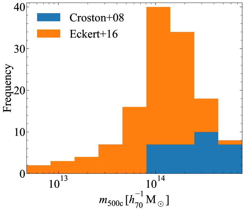
Figure 1: Stacked histogram for the masses of the haloes in our sample. The XXL-100-GC (Eckert et al., 2016) data probe lower masses than the REXCESS (Croston et al., 2008) data set, but it is clear that most of the haloes are clusters of galaxies with $m_{\mathrm{500c,obs}}>${10}^{14}\text{\,}$Msun{\mathrm{M_{\odot}}}$$$.

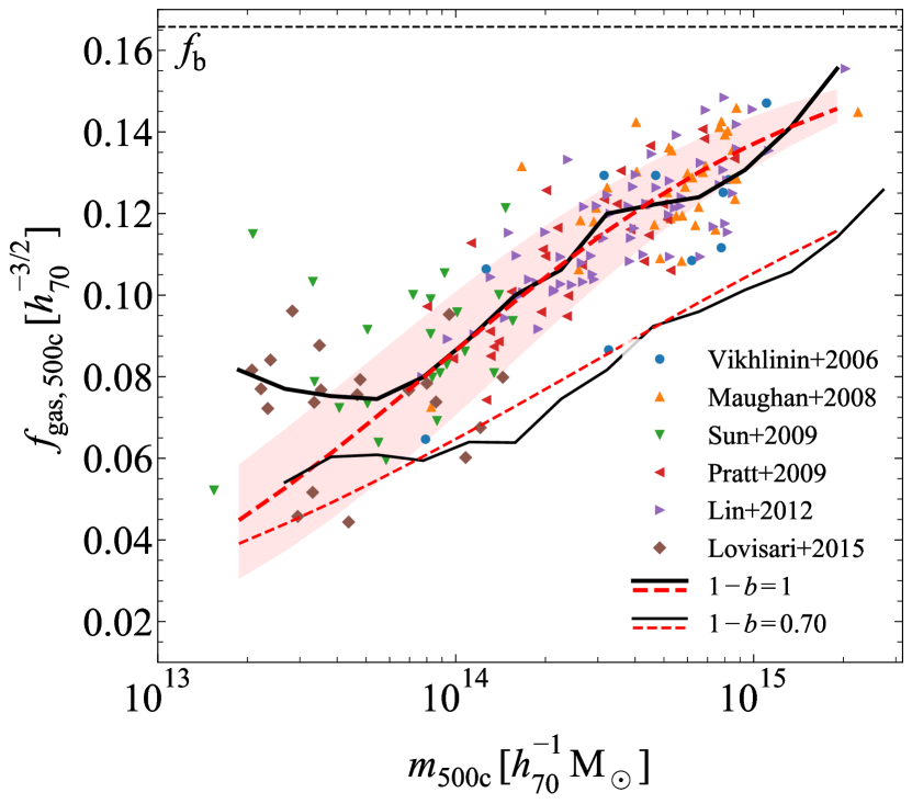
Figure 2: The X-ray hydrostatic gas fractions as a function of halo mass. The different data sets are explained in the text. The median $f_{\mathrm{gas,500c}}-m_{\mathrm{500c,obs}}$ relation (black, solid lines) and the best fit (red, dashed lines) using Eq. 25 are shown. We indicate the 15^th and 85^th percentile range by the red shaded region. We show the hydrostatic (thick lines) and bias corrected ($1-b=0.7$, thin lines) relations. Since, in the latter case, halo masses increase more than the gas masses, under the assumption of the best-fit beta profile to the hot gas density profiles, the gas fractions shift down. The fits deviate at low masses because we force $f_{\mathrm{gas,500c}}\to 0$ for $m_{\mathrm{500c,obs}}\to 0$.

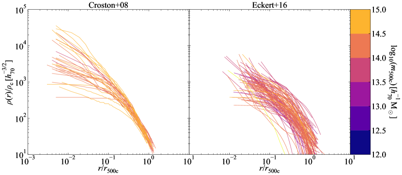
Figure 3: The hot gas density profiles inferred from the X-ray observations colour-coded by $m_{\mathrm{500c,obs}}$. The left-hand panel shows the profiles from the REXCESS sample (31 nearby clusters with $${10}^{14}$\lesssim m_{\mathrm{500c,obs}}/$$Msun{\mathrm{M_{\odot}}}$$\lesssim${10}^{15}$$, Croston et al., 2008) and the right-hand panel from the XXL survey (100 bright clusters with $${10}^{13}$\lesssim m_{\mathrm{500c,obs}}/$$Msun{\mathrm{M_{\odot}}}$$\lesssim${10}^{15}$$, Eckert et al., 2016).

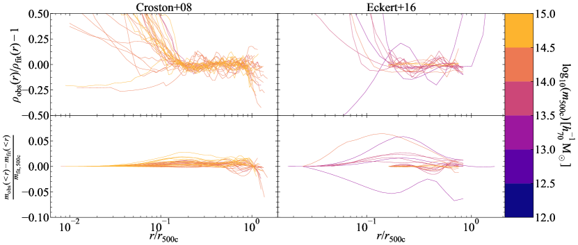
Figure 4: Top row Residual of beta profile fits to the hot gas density profiles in Fig. 3. The left-hand panel shows the residuals for the REXCESS sample (Croston et al., 2008) and the right-hand panel for the XXL-100-GC sample (Eckert et al., 2016). The fits are accurate within $\sim$10\text{\,}\mathrm{\char 37\relax}$$ for the range $0.1<r/r_{\mathrm{500c,obs}}<1$, with larger scatter in the inner region, where the beta profile generally underestimates the total mass. For the XXL-100-GC sample (Eckert et al., 2016) we binned the profiles into 20 mass bins since there is a large scatter in the individual ones. We only fit the profile at radial ranges where there is data for all the individual profiles in the bin. Bottom row Residual of beta profile fits to the cumulative mass fraction. The total amount of mass within the inner region is negligible compared to the total mass in the profile. In the inner regions the observed profiles always yield higher masses than the fits because of the core of the beta profile. We reproduce the total mass $m_{\mathrm{gas,500c}}$ of the individual density profiles by construction.

We choose to constrain the halo model using observations of the hot, X-ray emitting gas in groups and clusters of galaxies, since these objects provide the dominant contribution to the power spectrum at our scales of interest and their baryon content is dominated by hot plasma.

We combine two data sets of X-ray observations with XMM-Newton of clusters for which the individually measured electron density profiles were available, namely REXCESS (Croston et al., 2008) and the XXL survey (more specifically the XXL-100-GC subset, Pacaud et al., 2016; Eckert et al., 2016). This gives a total of 131 ($31+100$) unique groups and clusters (there is no overlap between the two data sets) with masses ranging from $m_{\mathrm{500c,obs}}\approx$1\text{\times}{10}^{13}\text{\,}$Msun{\mathrm{M_{\odot}}}$$$ to $m_{\mathrm{500c,obs}}\approx$2\text{\times}{10}^{15}\text{\,}$Msun{\mathrm{M_{\odot}}}$$$, with the XXL sample probing lower masses, as can be seen in Fig. 1. We extend our data with more sets of observations for the hydrostatic gas fraction of groups and clusters of galaxies, as shown in Fig. 2. We use a set of hydrostatic masses determined from Chandra archival data (Vikhlinin et al., 2006; Maughan et al., 2008; Sun et al., 2009; Lin et al., 2012) and from the NORAS and REFLEX (of which REXCESS is a subset) surveys (Pratt et al., 2009; Lovisari et al., 2015).

REXCESS consists of a representative sample of clusters from the REFLEX survey (Böhringer et al., 2007). It includes clusters of all dynamical states and aims to provide a homogeneous sampling in X-ray luminosity of clusters in the local Universe ($z<0.2$). Since all of the redshift bins are approximately volume limited (Böhringer et al., 2007), we do not expect significant selection effects for the massive systems ($m_{\mathrm{500c}}>${10}^{14}\text{\,}$\mathrm{\mathit{h}}^{-1}\,$Msun{\mathrm{M_{\odot}}}$$$$) as it has been shown by Chon & Böhringer (2017) that the lack of disturbed clusters in X-ray samples (Eckert et al., 2011) is generally due to their flux-limited nature. The XXL-100-GC sample is flux-limited (Pacaud et al., 2016) and covers a wider redshift range ($z\lesssim 1$). Since it is flux-limited, there is a bias to selecting more massive objects. At low redshifts, however, there is a lack of massive objects due to volume effects (Pacaud et al., 2016). From Chon & Böhringer (2017) we would also expect the sample to be biased to select relaxed systems.

Assuming an optically thin, collisionally-ionized plasma with a temperature $T$ and metallicity $Z$, the deprojected surface brightness profile can be converted into a 3-D electron density profile $n_{e}$, which is the source of the thermal bremsstrahlung emission (Sarazin, 1986). For the REXCESS sample, the spectroscopic temperature within $r_{\mathrm{500c,obs}}$ was chosen with the metallicity also deduced from a spectroscopic fit, whereas for the XXL sample the average temperature within $r<$300\text{\,}\mathrm{k}\mathrm{p}\mathrm{c}$$ was used with a metallicity of $Z=$0.3\text{\,}\mathrm{Z_{\odot}}$$. We get the corresponding hydrogen and helium abundances by interpolating between the sets of primordial abundances, $(X_{0},Y_{0},Z_{0})=(0.75,0.25,0)$, and of solar abundances, $(\mathrm{X_{\odot}},\mathrm{Y_{\odot}},\mathrm{Z_{\odot}})=(0.7133,0.2735,0.0132)$. We then find $(X,Y,Z)=(0.73899,0.25705,0.00396)$ for $Z=$0.3\text{\,}\mathrm{Z_{\odot}}$$. To convert this electron density into the total density, we will assume these interpolated abundances, since in general for clusters the metallicity $Z\approx$0.3\text{\,}\mathrm{Z_{\odot}}$=0.00396$ (Voit, 2005; Grevesse et al., 2007). This is also approximately correct for the Croston et al. (2008) data, since for their systems the median metallicity (bracketed by 15^th and 85^th percentiles) is $Z/$\mathrm{Z_{\odot}}$=0.27\begin{subarray}{c}+0.09\\ -0.05\end{subarray}$. Moreover, we assume the gas to be fully ionized. We know that the total gas density is given by

$$\rho_{\mathrm{gas}} =\mu m_{\text{H\,{}}}(n_{e}+n_{\text{H\,{}}}+n_{\text{He\,{}}})$$

$$=\frac{1+Y/X}{2+3Y/(4X)}\frac{2+3Y/(4X)}{1+Y/(2X)}m_{\text{H\,{}}}n_{e}$$

$$\approx 0.6\cdot 1.93\,m_{\text{H\,{}}}n_{e}$$ (24)

This results in the gas density profiles shown in Fig. 3. It is clear that at large radii the scatter is smaller for more massive systems. We bin the XXL data in 20 mass bins as the individual profiles have a large scatter at fixed radius. For each mass bin we only include the radial range where each profile in the bin is represented.

The two surveys derived the halo mass $m_{\mathrm{500c,obs}}$ differently. For REXCESS, the halo masses for the whole sample were determined from the $m_{\mathrm{500c,obs}}-Y_{\mathrm{X}}$ relation of Arnaud et al. (2007), where $Y_{\mathrm{X}}=m_{\mathrm{gas,500c}}\,T_{\mathrm{X}}$ is the thermal energy content of the intracluster medium (ICM). Arnaud et al. (2007) determined $m_{\mathrm{500c,obs}}$ under the assumption of spherical symmetry and hydrostatic equilibrium (see e.g. Voit, 2005). Eckert et al. (2016) take a different route. They determine halo masses using the $m_{\mathrm{500c,obs}}-T_{\mathrm{X}}$ relation calibrated to weak lensing mass measurements of 38 clusters that overlap with the CFHTLenS shear catalog, as described in Lieu et al. (2016). As a result, the REXCESS halo mass estimates rely on the assumption of hydrostatic equilibrium, whereas Eckert et al. (2016) actually find a hydrostatic bias $m_{\mathrm{X-ray}}/m_{\mathrm{WL}}=1-b=0.72$, consistent with the analyses of Von der Linden et al. (2014) and Hoekstra et al. (2015). Recently, Umetsu et al. (2019) used the Hyper Suprime-Cam (HSC) survey shear catalog, which overlaps the XXL-North field almost completely, to measure weak lensing halo masses with a higher limiting magnitude and, hence, number density of source galaxies than CHFTLenS. They do not rederive the gas fractions of Eckert et al. (2016), but they note that their masses are systematically lower by a factor $\approx 0.75$ than those derived in Lieu et al. (2016), a finding which is consistent with Lieu et al. (2017), who find a factor $\approx 0.72$. These lower weak lensing halo masses result in a hydrostatic bias of $b<0.1$.

To obtain a consistent analysis, we scale the halo masses from Eckert et al. (2016) back onto the hydrostatic $f_{\mathrm{gas,500c}}-m_{\mathrm{500c,obs}}$ relation, which we show in Fig. 2. We thus assume halo masses derived from the assumption of hydrostatic equilibrium. It might seem strange to take the biased result as the starting point of our analysis. However, we argue that this is an appropriate starting point. First, current estimates for the hydrostatic bias range from $0.58\pm 0.04\lesssim 1-b\lesssim 0.71\pm 0.10$ corresponding to the results from Planck SZ cluster counts (Planck Collaboration et al., 2016b; Zubeldia & Challinor, 2019), or $0.688\pm 0.072\lesssim 1-b\lesssim 0.80\pm 0.14$ from weak lensing mass measurements of Planck clusters (Von der Linden et al., 2014; Hoekstra et al., 2015; Medezinski et al., 2018). Second, we are not able to determine the mass dependence of the relation for groups of galaxies from current observations. We will check how our results change when assuming a constant hydrostatic bias of $1-b=0.7$ in § 5.5. The thin, black line in Fig. 2 shows the shift in the $f_{\mathrm{gas,500c}}(m_{\mathrm{500c,obs}})$ relation when assuming this constant hydrostatic bias.

We fit the cluster gas density profiles with beta profiles, following Eq. 14, within $[0.15,1]\,r_{\mathrm{500c,obs}}$, excising the core as usual in the literature, since it can deviate from the flat slope in the beta profile. In observations, it is common to assume a sum of different beta profiles to capture the slope in the inner $0.15r_{\mathrm{500c,obs}}$. However, we correct for the mass that we miss in the core by fixing the normalization to reproduce the total gas mass of the profile, which is captured by the gas fraction $f_{\mathrm{gas,500c}}$. (This is equivalent to redistributing the small amount of mass that we would miss in the core to larger scales.) The slope at large radii, $\beta$, and the core radius, $r_{\mathrm{c}}$, are the final two parameters determining the profile. We show the residuals of the profile fits in Fig. 4 where we also include the residuals of the cumulative mass profile. It is clear from the residuals in the top panels of Fig. 4 that the beta profile cannot accurately capture the inner density profile of the hot gas. Arnaud et al. (2010) show that the inner slope can vary from shallow to steep in going from disturbed to relaxed or cool-core clusters. This need not concern us because the deviations from the fit occur at such small radii that they will not be able to significantly affect the power at our scales of interest where the normalization of $\hat{\rho}_{\mathrm{gas}}(k)$ and, thus, the total mass of the hot gas component is the important parameter. In the bottom panel of Fig. 4 we show the residuals for the cumulative mass. The left-hand panel of the figure clearly shows that we force $m_{\mathrm{gas,500c}}$ in the individual profiles to equal the observed mass.

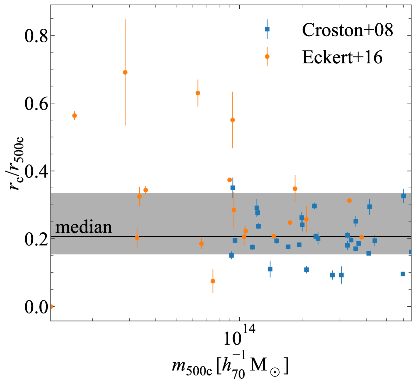
Figure 5: The mass dependence of the core radius $r_{\mathrm{c}}$ of the beta hot gas density profile fits, Eq. 14. We indicate the 15^th and 85^th percentiles with the gray shaded region and the median by the solid line. The error bars indicate the standard deviation in the best-fit parameter. We have binned the Eckert et al. (2016) sample into 20 mass bins. There is no clear mass dependence.

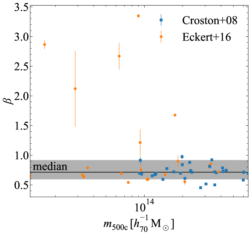
Figure 6: As Fig. 5 but for the slope $\beta$ of the beta hot gas density profile fits, Eq. 14.

We show the core radii, $r_{\mathrm{c}}$, and slopes, $\beta$, that we fit to our data set in Figs. 5 and 6, respectively. There is no clear mass dependence in the both of the fit parameters. Thus, we decided to use the median value for both parameters for all halo masses. This significantly simplifies the model, keeping the total number of parameters low.

We show the hydrostatic gas fractions from our observational data in Fig. 2. We fit the median $f_{\mathrm{gas,500c}}-m_{\mathrm{500c,obs}}$ relation with a sigmoid-like function given by

$$f_{\mathrm{gas,500c}}(m_{\mathrm{500c,obs}})=\frac{\Omega_{\mathrm{b}}/\Omega_{\mathrm{m}}}{2}\left(1+\tanh\left(\frac{\log_{10}(m_{\mathrm{500c,obs}}/m_{\mathrm{t}})}{\alpha}\right)\right)\,,$$ (25)

under the added constraint

$$f_{\mathrm{gas,500c}}(m_{\mathrm{500c,obs}})\leq f_{\mathrm{b}}-f_{\mathrm{\star,500c}}(m_{\mathrm{500c,obs}})\,.$$ (26)

The function has as free parameters the turnover mass, $m_{\mathrm{t}}$, and the sharpness of the turnover, $\alpha$. We fix the gas fraction for $m_{\mathrm{500c,obs}}\to\infty$ to the cosmic baryon fraction $f_{\mathrm{b}}=\Omega_{\mathrm{b}}/\Omega_{\mathrm{m}}\approx$0.166$$, which is what we expect for deep potential wells and what we also see for the highest-mass clusters. However, we shift down the final $f_{\mathrm{gas,500c}}(m_{\mathrm{500c,obs}})$ relation at halo masses where the cosmic baryon fraction would be exceeded after including the stellar contribution. We also fix the gas fraction for $m\to 0$ to 0 since we know that low-mass dwarfs eject their baryons easily and are mainly dark matter dominated (e.g. Silk & Mamon, 2012; Sawala et al., 2015). Moreover, their virial temperatures are too low for them to contain X-ray emitting gas. Fixing $f_{\mathrm{gas,500c}}(m\to 0)=0$ is probably not optimal, especially since we know that the lower mass haloes will contain a significant warm gas ($${10}^{4}\text{\,}\mathrm{K}$\lesssim T\lesssim${10}^{6}\text{\,}\mathrm{K}$$) component which should increase their baryonic mass. However, since we will use our freedom in correcting the gas fraction at $r_{\mathrm{h}}$ by assuming profiles outside $r_{\mathrm{500c,obs}}$, this choice should not significantly impact our results as we already discussed at the end of § 2.3.1. For our scales of interest, the shape of the profiles of low-mass systems will not matter as much as their total mass. Forcing the gas fraction to go to 0 for low halo masses causes a deviation from the observations at low halo masses. However, at low halo mass the X-ray observations will always be biased to systems with high gas masses, since these will have the highest X-ray luminosities.

In Fig. 2 we also show fits to the data $f_{\mathrm{gas,500c}}-m_{\mathrm{500c,obs}}$ relation assuming a constant hydrostatic mass bias of $\frac{m_{\mathrm{hydro}}}{m_{\mathrm{true}}}=1-b=0.7$. In § 5.5 we discuss how we compute this relation and the influence of this assumption on our results.

4 Model density components

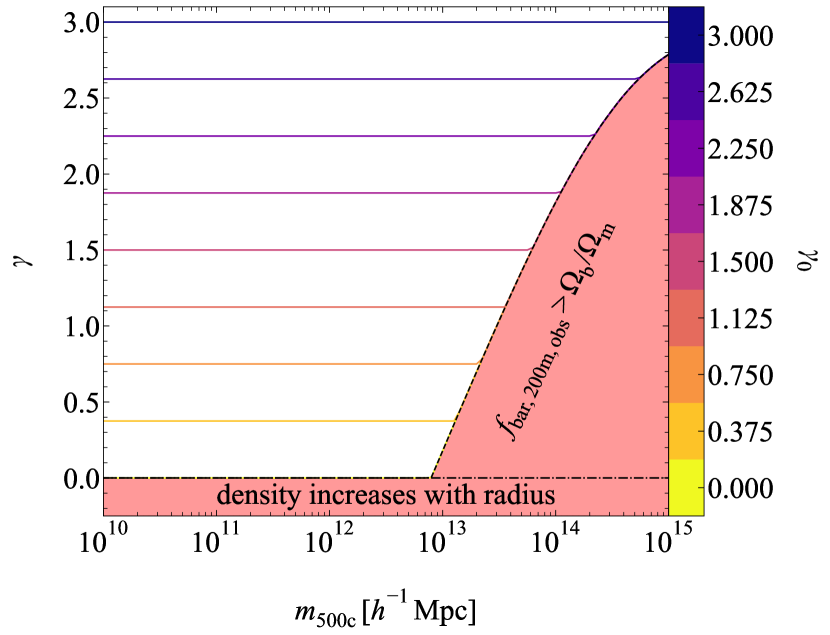
Figure 7: The allowed values for the extrapolated slope $\gamma$ of the beta density profile, Eq. 14, as a function of halo mass $m_{\mathrm{500c,obs}}$. We colour each line by the value $\gamma_{0}=\gamma(m_{\mathrm{500c,obs}}\to 0)$. Since we extrapolate haloes to $r_{\mathrm{200m,obs}}$, the most massive haloes would contain too many baryons if $\gamma$ would be too small. Hence, for each halo mass, we compute the limiting $\gamma$ for which the halo is baryonically closed at $r_{\mathrm{200m,obs}}$. This limit is indicated by the dashed line. For each halo mass only slopes steeper than this limit are allowed.

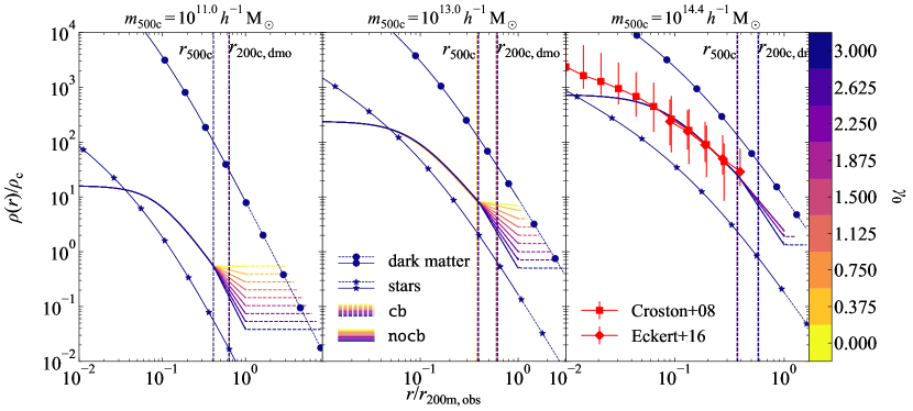
Figure 8: Model density profiles for $m_{\mathrm{500c,obs}}=${10}^{11}\text{\,}$\mathrm{\mathit{h}}^{-1}\,$Msun{\mathrm{M_{\odot}}}$$$$ (left panel), $m_{\mathrm{500c,obs}}=${10}^{13}\text{\,}$\mathrm{\mathit{h}}^{-1}\,$Msun{\mathrm{M_{\odot}}}$$$$ (middle panel), and $m_{\mathrm{500c,obs}}=$e14.4\text{\,}$\mathrm{\mathit{h}}^{-1}\,$Msun{\mathrm{M_{\odot}}}$$$$ (right panel). In the right panel, we also show the median hot gas density profiles inferred from REXCESS (red, connected squares, Croston et al., 2008) and XXL-100-GC (red, connected diamonds, Eckert et al., 2016) for a sample with the same median halo mass. The error bars indicate the 15^th and 85^th percentile range for each radial bin. The lines are colour-coded by $\gamma_{0}\equiv\gamma(m_{\mathrm{500c}}\to 0)$, the extrapolated power-law slope of the hot gas density profiles between $r_{\mathrm{500c,obs}}$ and $r_{\mathrm{200m,obs}}$, with lower values of $\gamma_{0}$ corresponding to flatter slopes. All profiles assume the best-fit beta profile up to $r_{\mathrm{500c,obs}}$. Between $r_{\mathrm{500c,obs}}$ and $r_{\mathrm{200m,obs}}$ the profiles are extrapolated with a power-law slope of $\gamma$. In the case of $\mathtt{nocb}$ (solid, coloured lines), we cut off the profiles at the halo definition $r_{\mathrm{200m,obs}}$, at which point the halo baryon fraction may be smaller than $\Omega_{\mathrm{b}}/\Omega_{\mathrm{m}}$. For the case $\mathtt{cb}$ (dashed, coloured lines), we extrapolate the hot gas density profile with a uniform profile until the cosmic baryon fraction is reached. For the case $\mathtt{cb}$ of the dark matter (dashed, connected circles) and stellar satellite (dashed, connected stars) profiles, we only show the models with $\gamma_{0}=3$, for the other values of $\gamma_{0}$ the maximum radius equals that of the corresponding hot gas profile.

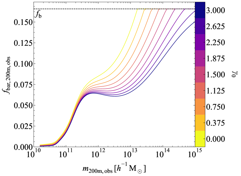
Figure 9: The halo baryon fraction at $r_{\mathrm{200m,obs}}$ as a function of halo mass $m_{\mathrm{200m,obs}}$. The baryon fraction $f_{\mathrm{bar,200m,obs}}$ is the same for both model $\mathtt{nocb}$, which effectively assumes that the missing halo baryons are redistributed far beyond $r_{\mathrm{200m,obs}}$ on linear scales, and model $\mathtt{cb}$, which adds the missing halo baryons in a uniform profile outside but near $r_{\mathrm{200m,obs}}$. The lines are colour-coded by $\gamma_{0}\equiv\gamma(m_{\mathrm{500c}}\to 0)$, the extrapolated power-law slope of the hot gas density profiles between $r_{\mathrm{500c,obs}}$ and $r_{\mathrm{200m,obs}}$, with lower values of $\gamma_{0}$ corresponding to flatter slopes. The shape is set by the observed constraints on the baryon fractions at $r_{\mathrm{500c,obs}}$. As $\gamma_{0}$ decreases to 0, the halo baryon fractions increase. The knee at $m_{\mathrm{200m,obs}}\approx${10}^{12}\text{\,}$\mathrm{\mathit{h}}^{-1}\,$Msun{\mathrm{M_{\odot}}}$$$$ is caused by the peak of the stellar mass fractions. The decreased range of possible baryon fractions for low-mass haloes is the consequence of their low gas fractions and the fixed prescription for the stellar component.

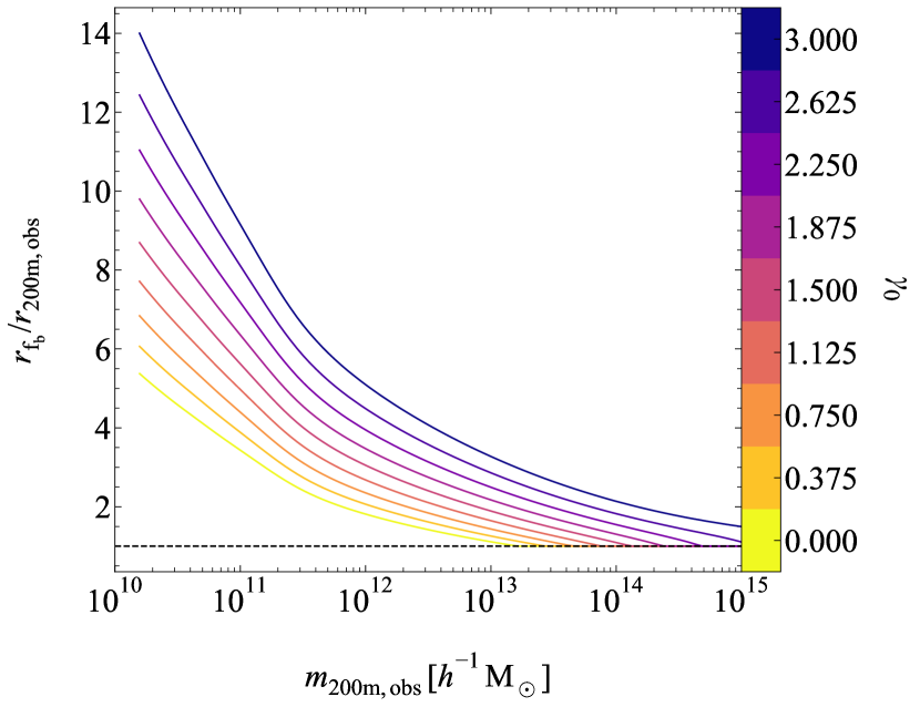
Figure 10: The radius where the cosmic baryon fraction is reached in units of $r_{\mathrm{200m,obs}}$ as a function of halo mass $m_{\mathrm{200m,obs}}$ for model $\mathtt{cb}$, which adds the missing halo baryons in a uniform profile outside $r_{\mathrm{200m,obs}}$. The lines are colour-coded by $\gamma_{0}\equiv\gamma(m_{\mathrm{500c}}\to 0)$, the extrapolated power-law slope of the hot gas density profiles between $r_{\mathrm{500c,obs}}$ and $r_{\mathrm{200m,obs}}$, with lower values of $\gamma_{0}$ corresponding to flatter slopes. As $\gamma_{0}$ decreases to 0, the cosmic baryon fraction is reached closer to the halo radius $r_{\mathrm{200m,obs}}$.

We determined the best-fit parameters for the beta profile, Eq. 14, in § 3. The only remaining free parameter in our model is now the slope $\gamma$ of the extrapolated profile outside $r_{\mathrm{500c,obs}}$. As we explained in § 3, not all values of $\gamma$ are allowed for each halo mass $m_{\mathrm{500c,obs}}$, since the most massive haloes contain a significant fraction of their total baryon budget inside $r_{\mathrm{500c,obs}}$. Consequently, these haloes need steeper slopes $\gamma$, since otherwise they would exceed the cosmic baryon fraction before they reach the halo radius $r_{\mathrm{200m,obs}}$. We thus determine the relation $\gamma_{\mathrm{min}}(m_{\mathrm{500c,obs}})$ that limits the extrapolated slope such that, given the best-fit beta profile parameters, the halo reaches exactly the cosmic baryon fraction at $r_{\mathrm{200m,obs}}$. For each halo mass only slopes steeper than this limiting value are allowed. We show the resulting relation $\gamma_{\mathrm{min}}(m_{\mathrm{500c,obs}})$ in Fig. 7. We colour the curves by $\gamma_{0}=\gamma(m_{\mathrm{500c,obs}}\to 0)$. Since low-mass haloes have low baryon fractions at $r_{\mathrm{500c,obs}}$, we find that all values of $\gamma_{0}$ are allowed. For the most massive haloes, only the steepest slopes $\gamma\gtrsim 2.8$ are allowed. The handful of observations that are able to probe clusters out to $r_{\mathrm{200m,obs}}$ indeed find that the slope steepens in the outskirts (Ghirardini et al., 2019).

Now we have all of the ingredients of our model at hand. We show the resulting profiles for our different matter components for 3 halo masses in Fig. 8. We show both the $\mathtt{nocb}$ and $\mathtt{cb}$ models, where the latter are just the former extended beyond $r_{\mathrm{200m,obs}}$ until the cosmic baryon fraction is reached. We colour the curves by $\gamma_{0}$. Given $\gamma_{0}$, the actual value of the slope $\gamma$ for each halo mass can be determined by following the tracks in Fig. 7 from low to high halo masses, e.g. for the $m_{\mathrm{500c,obs}}=${10}^{15}\text{\,}$\mathrm{\mathit{h}}^{-1}\,$Msun{\mathrm{M_{\odot}}}$$$$ halo all slopes $\gamma_{0}\leq 2.8$ correspond to the actual slope $\gamma=2.8$. Besides the hot gas profiles, we also show the dark matter and stellar (satellite, since the central is modelled as a delta function) profiles. These profiles only depend on the value $\gamma_{0}$ through their maximum radius, since the halo radius $r_{\mathrm{h}}$ is determined by how fast the cosmic baryon fraction is reached and thus depends on $\gamma_{0}$.

It is clear that models with flatter slopes reach their baryon budget at smaller radii. These models will thus capture the influence of a compact baryon distribution on the matter power spectrum. We show the halo baryon fraction at $r_{\mathrm{200m,obs}}$ for different values of $\gamma_{0}$ in Fig. 9. The main shape of the gas fractions at $r_{\mathrm{200m,obs}}$ is set by the constraints on the gas fractions at $r_{\mathrm{500c,obs}}$. The group-size haloes have the largest spread in baryon fraction with changing slope $\gamma_{0}$. Our model is thus able to capture a large range of different baryon contents for haloes that all reproduce the observations at $r_{\mathrm{500c,obs}}$. The baryon fractions rise steeply between $${10}^{11}$<m_{\mathrm{200m,obs}}/($$\mathrm{\mathit{h}}^{-1}\,$Msun{\mathrm{M_{\odot}}}$$$)<${10}^{12}$$ due to the peak in the stellar mass fraction in this halo mass range. For the low-mass haloes, the spread in baryon fraction is smaller at $r_{\mathrm{200m,obs}}$ because we hold the stellar component fixed in our model and their gas fractions are low. As a result, the low-mass systems do not differ much in the $\mathtt{nocb}$ model. (In the $\mathtt{cb}$ model they will differ due to the different halo radii $r_{\mathrm{h}}$ where the cosmic baryon fraction is reached.) For the slope $\gamma$ between $03$ we will have $\approx$2050\text{\,}\mathrm{\char 37\relax}$$ of the total baryons in the Universe outside haloes in the $\mathtt{nocb}$ model.

We have checked that the density profiles with varying $\gamma_{0}$ for for haloes with $${10}^{14}$<m_{\mathrm{500c,obs}}/$$\mathrm{\mathit{h}}^{-1}\,$Msun{\mathrm{M_{\odot}}}$$$<${10}^{15}$$ only cause a maximum deviation of $\approx\pm$5\text{\,}\mathrm{\char 37\relax}$$ in the surface brightness profiles for projected radii $R<r_{\mathrm{500c,obs}}$ compared to the fiducial model with $\gamma_{0}=3\beta$. This variation is within the error on the surface brightness counts and the density profiles with varying $\gamma_{0}$ are thus indistinguishable from the fiducial model in the investigated mass range. For haloes with $m_{\mathrm{500c,obs}}\leq${10}^{14}\text{\,}$\mathrm{\mathit{h}}^{-1}\,$Msun{\mathrm{M_{\odot}}}$$$$, the deviations increase for lower values of $\gamma_{0}$, reaching $10\text{\,}\mathrm{\char 37\relax}$ for $\gamma_{0}=1.5$ and $m_{\mathrm{500c,obs}}=${10}^{13}\text{\,}$\mathrm{\mathit{h}}^{-1}\,$Msun{\mathrm{M_{\odot}}}$$$$, but the observed hot gas density profiles at these halo masses also show a larger scatter.

We also have the $\mathtt{cb}$ model where we force all haloes to include all of the missing baryons in their outskirts. In Fig. 10 we show how extended the baryon distribution needs to be in the $\mathtt{cb}$ case as a function of the slope $\gamma_{0}$. The variations in the power-law slope paired with the $\mathtt{cb}$ and $\mathtt{nocb}$ models allow us to investigate the influence on the matter power spectrum of a wide range of possible baryon distributions that all reproduce the available X-ray observations for clusters with $m_{\mathrm{500c,obs}}\geq${10}^{14}\text{\,}$\mathrm{\mathit{h}}^{-1}\,$Msun{\mathrm{M_{\odot}}}$$$$.

5 Results

In this section we show the results and predictions of our model for the matter power spectrum and we discuss their implications for future observational constraints. First, we show the influence of assuming different distributions for the unobserved hot gas in § 5.1. We show the influence of correcting observed halo masses to the dark matter only equivalent halo masses in order to obtain the correct halo abundances in § 5.2. In § 5.3, we show which halo masses dominate the power spectrum for which wavenumbers. Finally, we show the influence of varying the best-fit observed profile parameters in § 5.4 and we investigate the effects of a hydrostatic bias in the halo mass determination in § 5.5.

5.1 Influence of the unobserved baryon distribution

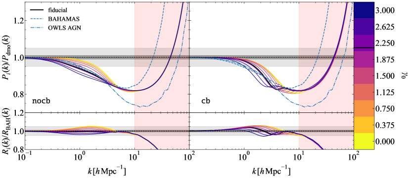
Figure 11: Top row The ratio of our halo model power spectra with baryons to the corresponding dark matter only prediction. The dark and light gray bands indicate the $1\text{\,}\mathrm{\char 37\relax}$ and $5\text{\,}\mathrm{\char 37\relax}$ intervals. The left-hand panel shows model $\mathtt{nocb}$, which effectively assumes that the baryons missing from haloes are redistributed far beyond $r_{\mathrm{200m,obs}}$ on linear scales. The right-hand panel shows model $\mathtt{cb}$, which adds the missing halo baryons in a uniform profile outside but near $r_{\mathrm{200m,obs}}$. The red, lightly-shaded region for $k>$10\text{\,}$\mathrm{\mathit{h}}\,\mathrm{M}\mathrm{pc}^{-1}$$$ indicates the scales where our model is is not a good indicator of the uncertainty because the stellar component is not varied. We indicate our fiducial model, which simply extrapolates the best-fit beta profile to the hot gas density profiles of clusters, with a thick black line. The lines are colour-coded by $\gamma_{0}\equiv\gamma(m_{\mathrm{500c}}\to 0)$, the extrapolated power-law slope of the hot gas density profiles between $r_{\mathrm{500c,obs}}$ and $r_{\mathrm{200m,obs}}$, with lower values of $\gamma_{0}$ corresponding to flatter slopes. The clear difference between the $\mathtt{nocb}$ and $\mathtt{cb}$ models on large scales indicates that it is very important to know where the missing halo baryons end up. Placing the missing halo baryons in the vicinity of the haloes increases the power on large scales significantly for fixed $\gamma_{0}$. Our model is flexible enough, especially in the $\mathtt{nocb}$ case, to encompass the behaviour of both the bahamas (blue, dashed line) and OWLS (blue, dash-dotted line) simulations on large scales. Bottom row The ratio between the matter power spectra responses to baryons predicted by our models and the bahamas simulation. Both our fiducial models are within $\approx$5\text{\,}\mathrm{\char 37\relax}$$ of bahamas for $k<$10\text{\,}$\mathrm{\mathit{h}}\,\mathrm{M}\mathrm{pc}^{-1}$$$.

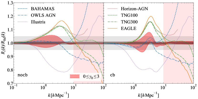
Figure 12: The ratio between the power spectrum response to baryons predicted by hydrodynamical simulations from the literature and our fiducial halo model, which simply extrapolates the best-fit beta profile to the hot gas density profiles of clusters. The dark and light gray bands indicate the $1\text{\,}\mathrm{\char 37\relax}$ and $5\text{\,}\mathrm{\char 37\relax}$ intervals. The left-hand panel shows model $\mathtt{nocb}$, which effectively assumes that the baryons missing from haloes are redistributed far beyond $r_{\mathrm{200m,obs}}$ on linear scales. The right-hand panel shows model $\mathtt{cb}$, which adds the missing halo baryons in a uniform profile outside but near $r_{\mathrm{200m,obs}}$. The red, lightly-shaded region for $k>$10\text{\,}$\mathrm{\mathit{h}}\,\mathrm{M}\mathrm{pc}^{-1}$$$ indicates the scales where our model is is not a good indicator of the uncertainty because the stellar component is not varied. The shaded red region shows the spread in our models for all values of $\gamma_{0}$, i.e. the extrapolated power-law slope of the hot gas density profiles between $r_{\mathrm{500c,obs}}$ and $r_{\mathrm{200m,obs}}$, with red lines indicating $\gamma_{0}=0$ (red, dashed line) and $\gamma_{0}=3$ (red, solid line). The blue lines indicate simulations that reproduce the hot gas fractions of clusters, i.e. bahamas (blue, dashed line, McCarthy et al., 2017) and OWLS AGN (blue, dash-dotted line, van Daalen et al., 2011). We show the higher-resolution but smaller-volume simulations which predict too large cluster gas fractions, i.e. EAGLE (orange, solid line, Hellwing et al., 2016), IllustrisTNG-100 and 300 (green, dashed and dash-dotted lines, respectively, Springel et al., 2017), Horizon-AGN (red, dotted line, Chisari et al., 2018). We also show the original Illustris result (purple, dotted line, Vogelsberger et al., 2014b), which underpredicts cluster gas fractions. Our empirical model encompasses the simulations that reproduce the cluster hot gas fractions on all scales $k\lesssim$5\text{\,}$\mathrm{\mathit{h}}\,\mathrm{M}\mathrm{pc}^{-1}$$$, but the other simulations fall outside of the allowed range.

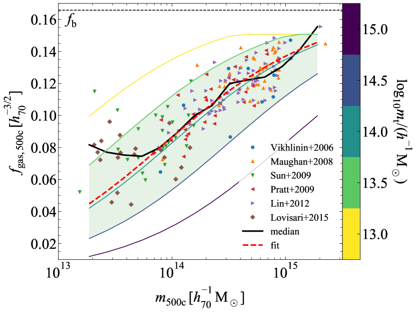
Figure 13: The X-ray hydrostatic gas fractions as a function of halo mass, as in Fig. 2. The curves show the sigmoid-like fit from Eq. (25) with the best-fit value for $\alpha=1.35$, coloured by the value $\log_{10}m_{\mathrm{t}}/($$\mathrm{\mathit{h}}^{-1}\,$Msun{\mathrm{M_{\odot}}}$$$)\in\{13,13.5,14,14.5,15\}$ (the best-fit value is 13.94). The shaded green region indicates the area that is broadly in agreement with observations.

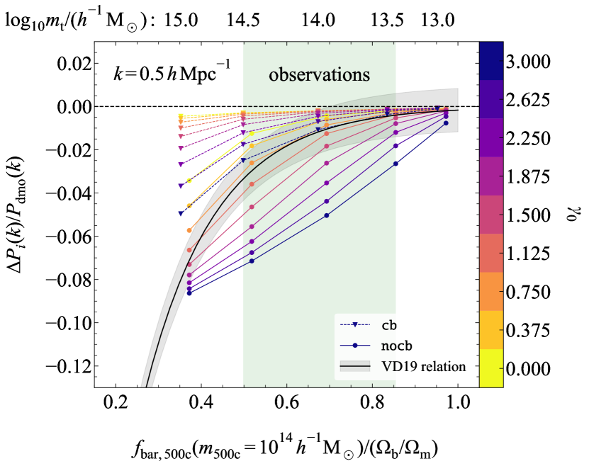
Figure 14: The power suppression due to the inclusion of baryons at the fixed scale $k=$0.5\text{\,}$\mathrm{\mathit{h}}\,\mathrm{M}\mathrm{pc}^{-1}$$$ as a function of the baryon fraction of haloes with $m_{\mathrm{500c,obs}}=${10}^{14}\text{\,}$\mathrm{\mathit{h}}^{-1}\,$Msun{\mathrm{M_{\odot}}}$$$$. The shaded green region indicates the gas fractions that broadly agree with observations. The $\mathtt{cb}$ (dashed, connected triangles) and $\mathtt{nocb}$ (connected circles) models are coloured by $\gamma_{0}$, i.e. the value of the extrapolated power-law slope of the hot gas density profiles between $r_{\mathrm{500c,obs}}$ and $r_{\mathrm{200m,obs}}$. We show the relation found by van Daalen et al. (2019) for hydrodynamical simulations and its $\pm$1\text{\,}\mathrm{\char 37\relax}$$ variation (black line with grey, shaded region). We indicate the value of $\log_{10}m_{\mathrm{t}}/($$\mathrm{\mathit{h}}^{-1}\,$Msun{\mathrm{M_{\odot}}}$$$)$ in Eq. (25) along the top x-axis. Both our model and VD19 predict a positive correlation between the power suppression at fixed scale and the halo baryon fraction at fixed halo mass. However, it is clear that our model allows for a larger range in possible power suppression at fixed halo baryon fraction than is found in the simulations.

In this section, we will investigate the influence of the distribution of the unobserved baryons inside and outside haloes on the matter power spectrum. Since we currently have only a very tenuous grasp of the whereabouts of the missing baryons, it is important to explore how their possible distribution impacts the matter power spectrum.

As stated in § 2.3.1, our model is characterized by the extrapolated power-law slope $-\gamma$ for the hot gas density profile and by whether we assume the missing halo baryons to reside in the vicinity of the halo (model $\mathtt{cb}$) or not (model $\mathtt{nocb}$). As explained in § 2.3.1, these two types of models only differ in $\hat{\rho}(k|m)$ due to the inclusion of more mass outside the traditional halo definition of $r_{\mathrm{200m,obs}}$ in the $\mathtt{cb}$ case (see Figs. 8, 10). When discussing our model predictions for the power spectrum, we consider the range $$0.1\text{\,}$\mathrm{\mathit{h}}\,\mathrm{M}\mathrm{pc}^{-1}$$\leq k\leq$5\text{\,}$\mathrm{\mathit{h}}\,\mathrm{M}\mathrm{pc}^{-1}$$$ to be the vital regime since future surveys will gain their optimal signal-to-noise for $k\approx$1\text{\,}$\mathrm{\mathit{h}}\,\mathrm{M}\mathrm{pc}^{-1}$$$ (Amendola et al., 2018).

We show the response of the matter power spectrum to baryons for the $\mathtt{nocb}$ and $\mathtt{cb}$ models in, respectively, the top-left and top-right panels of Fig. 11. The lines are coloured by the assumed value of $\gamma_{0}$. We indicate our fiducial model, which extrapolates the best-fit $\beta=0.71^{+0.20}_{-0.12}$, i.e. $\gamma_{0}=3\beta=2.14$, from the X-ray observations, with the thick, black line. All models show a suppression of power on large scales with respect to the DMO prediction. All of our models have an upturn in the response for $k\gtrsim$10\text{\,}$\mathrm{\mathit{h}}\,\mathrm{M}\mathrm{pc}^{-1}$$$ and and enhancement of power for $k\gtrsim$50\text{\,}$\mathrm{\mathit{h}}\,\mathrm{M}\mathrm{pc}^{-1}$$$ due to the stellar component. This upturn is not present in other halo model approaches that only modify the dark matter profiles (e.g. Smith et al., 2003; Mead et al., 2015). We shade the region $k>$10\text{\,}$\mathrm{\mathit{h}}\,\mathrm{M}\mathrm{pc}^{-1}$$$ in red because the range in responses of our model does not span the range allowed by observations there. On the contrary, on these small scales all of our models behave the same, since the hot gas is completely determined by the best-fit beta profile to the X-ray observations, and the stellar component is held fixed.

The total amount of power suppression at large scales depends sensitively on the halo baryon fractions, since models with the highest values of $\gamma_{0}$ also have the lowest baryon fractions $f_{\mathrm{bar,200m,obs}}$ at all halo masses (see Fig. 9). Our results confirm the predictions from hydrodynamical simulations, which have shown similar trends (van Daalen et al., 2011; van Daalen et al., 2019; Hellwing et al., 2016; McCarthy et al., 2017; Springel et al., 2017; Chisari et al., 2018). However, our results do not rely on the uncertain assumptions associated with subgrid models for feedback processes. Our phenomenological model simply requires that we reproduce the density profiles of clusters without any assumptions about the underlying physics that resulted in the profiles.

The $\mathtt{nocb}$ model, shown in the left-hand panel of Fig. 11, results in a larger spread of possible responses because the final total halo mass is not fixed to account for all the baryons as in $\mathtt{cb}$. The $\mathtt{nocb}$ models with the steepest extrapolated density profiles, i.e. the highest values for $\gamma_{0}$, function as upper limits on the response, since the missing halo baryons are in reality likely to reside in the vicinity of the haloes and because low-mass haloes likely contain more gas than predicted by our extrapolated relation. However, this gas may not be well described by our beta profile assumption derived from the hot gas properties of clusters. On the other hand, the $\mathtt{cb}$ models with flatter slopes (lower values for $\gamma_{0}$), shown in the right-hand panel of Fig. 11, function as lower limits on the response of the power spectrum to baryons, since it is likely that a significant fraction of the baryons does not reside inside haloes but rather in the diffuse, warm-hot, intergalactic medium (WHIM, as has been predicted by simulations and recently inferred from observations, see e.g. Cen & Ostriker, 1999; Dave et al., 2001; Nicastro et al., 2018). Hence, we find that the (minimum, fiducial, maximum) value of the minimum wavenumber for which the baryonic effect reaches $1\text{\,}\mathrm{\char 37\relax}$ is ($0.2$, $0.3$, $0.9$) $\mathrm{\mathit{h}}\,\mathrm{M}\mathrm{pc}^{-1}$ in the $\mathtt{nocb}$ models and ($0.5$, $0.8$, $1$) $\mathrm{\mathit{h}}\,\mathrm{M}\mathrm{pc}^{-1}$ in the $\mathtt{cb}$ models. The $5\text{\,}\mathrm{\char 37\relax}$ threshold is reached for ($0.5$, $0.8$, $2$) $\mathrm{\mathit{h}}\,\mathrm{M}\mathrm{pc}^{-1}$ and ($1$, $1.4$, $2$) $\mathrm{\mathit{h}}\,\mathrm{M}\mathrm{pc}^{-1}$, respectively, for the $\mathtt{nocb}$ and $\mathtt{cb}$ models.

We indicate the results from the bahamas simulation run $\mathtt{AGN\_TUNED\_nu0\_L400N1024\_WMAP9}$, which has been shown to reproduce a plethora of observations for massive systems (McCarthy et al., 2017; Jakobs et al., 2018), and the result for the OWLS AGN simulation (Schaye et al., 2010; van Daalen et al., 2011) which has been widely used as a reference model in weak lensing analyses and is also consistent with the observed cluster gas fractions (McCarthy et al., 2010). We show the ratio between our models and the bahamas prediction of the power spectrum response to the presence of baryons in the bottom row of Fig. 11. Our models encompass both the bahamas and OWLS predictions for $k\lesssim$5\text{\,}$\mathrm{\mathit{h}}\,\mathrm{M}\mathrm{pc}^{-1}$$$, which is the range of interest here. In the $\mathtt{cb}$ case, our models all predict less power suppression than the simulations on large scales $k\lesssim$1\text{\,}$\mathrm{\mathit{h}}\,\mathrm{M}\mathrm{pc}^{-1}$$$, which is most likely due to the fact that in the simulations there are actually baryons in the cosmic web that should not be accounted for by haloes, thus suggesting that models $\mathtt{nocb}$ may be more realistic. However, since there are no observational constraints on the location of the missing halo baryons, we cannot exclude the models $\mathtt{cb}$. We stress that we did not fit our model to reproduce these simulations. The overall similarity is caused by the simulations reproducing the measured X-ray hot gas fractions that we fit our model to.

In Fig. 12, we compare predictions for the power spectrum response to baryons from a large set of higher-resolution, but smaller-volume, cosmological simulations to the prediction of our fiducial model. We compare the EAGLE (Schaye et al., 2015; Hellwing et al., 2016), IllustrisTNG (Springel et al., 2017), Horizon-AGN (Chisari et al., 2018), and Illustris (Vogelsberger et al., 2014a) simulations. We can see that in all of these simulations, except for Illustris, which is known to have AGN feedback that is too violent on group and cluster scales (Weinberger et al., 2017), the baryonic suppression becomes significant only at much smaller scales than in OWLS, bahamas and our own model. From the halo model it is clear that the total baryon content of haloes, and thus the cluster gas fractions, are the dominant cause of baryonic power suppression on large scales $k\lesssim$1\text{\,}$\mathrm{\mathit{h}}\,\mathrm{M}\mathrm{pc}^{-1}$$$, since $\hat{\rho}(k|m)\to m$ there. Indeed, van Daalen et al. (2019) explicitly demonstrated the link between cluster gas fractions and power suppression on large scales for a large set of hydrodynamical simulations including these. Since bahamas and OWLS AGN reproduce the cluster hot gas fractions, they predict the same large-scale behaviour for the power spectrum response to baryons. However, the other small-volume, high-resolution simulations overpredict the baryon content of groups and clusters as was shown for EAGLE, IllustrisTNG, and Horizon-AGN by, respectively, Barnes et al. (2017), Barnes et al. (2018), and Chisari et al. (2018). We thus stress the importance of using simulations that are calibrated towards the relevant observations when training or comparing models aimed at predicting the matter power spectrum.

The small-scale behaviour of the power spectrum response to baryons is very sensitive to the stellar density profiles and as a result we see a large variation between the different simulation predictions in Fig. 12. As is shown by van Daalen et al. (2019), the small-scale power turnover in the simulations depends strongly on the resolution and subgrid physics of the simulation. We mentioned earlier that our model is fixed at these scales by the best-fit beta profiles to the X-ray observations and the fixed stellar component.

Recently, van Daalen et al. (2019) analyzed 92 hydrodynamical simulations, including all the ones shown in Fig. 12, and showed that there is a strong correlation between the total power suppression at a fixed scale $k\lesssim$1\text{\,}$\mathrm{\mathit{h}}\,\mathrm{M}\mathrm{pc}^{-1}$$$ and the baryon fraction at $r_{\mathrm{500c}}$ of haloes with $m_{\mathrm{500c}}=${10}^{14}\text{\,}$\mathrm{\mathit{h}}^{-1}\,$Msun{\mathrm{M_{\odot}}}$$$$. We investigate the same relation with our model. We show the different relations that we assume for the gas fraction $f_{\mathrm{gas,500c}}(m_{\mathrm{500c,obs}})$ in Fig. 13. For these relations we assume the best-fit value $\alpha=1.35$ from our fit to the observed gas fractions in Eq. (25), but we vary the turnover mass from its best-fit value of $\log_{10}m_{\mathrm{t}}/($$\mathrm{\mathit{h}}^{-1}\,$Msun{\mathrm{M_{\odot}}}$$$)=13.94$. Thus, we can capture a large range of possible gas fractions at $r_{\mathrm{500c,obs}}$, allowing us to encompass both the observed and the simulated gas fractions of $m_{\mathrm{500c,obs}}=${10}^{14}\text{\,}$\mathrm{\mathit{h}}^{-1}\,$Msun{\mathrm{M_{\odot}}}$$$$ haloes. For all these relations we then compute the power spectrum response due to the inclusion of baryons at the fixed scale $k=$0.5\text{\,}$\mathrm{\mathit{h}}\,\mathrm{M}\mathrm{pc}^{-1}$$$. We show the power suppression at this scale as a function of the halo baryon fraction in $m_{\mathrm{500c,obs}}=${10}^{14}\text{\,}$\mathrm{\mathit{h}}^{-1}\,$Msun{\mathrm{M_{\odot}}}$$$$ haloes in Fig. 14. Similarly to van Daalen et al. (2019), we find that higher baryon fractions at fixed halo mass result in smaller power suppression at fixed scale. In the $\mathtt{nocb}$ ($\mathtt{cb}$) case, the model with $\gamma_{0}=1.125$ ($\gamma_{0}=3$) most closely tracks the prediction from the hydrodynamical simulations. However, since our model has complete freedom for the gas density profile in the halo outskirts, the range of possible power suppression is much larger than that found in the simulations analyzed by van Daalen et al. (2019). The matter distribution in simulations is constrained by the subgrid physics that is assumed. Hence, relying only on simulation predictions might result in an overly constrained and model-dependent parameter space, since other subgrid recipes might result in differences in the matter distribution at large scales.

We conclude that the total baryon fraction of massive haloes is of crucial importance to the baryonic suppression of the power spectrum. Our model and hydrodynamical simulations that reproduce the cluster gas fractions are in general agreement about the total amount of suppression at scales $k\lesssim$5\text{\,}$\mathrm{\mathit{h}}\,\mathrm{M}\mathrm{pc}^{-1}$$$, with the exact amplitude depending on the details of the missing baryon distribution and varying by $\approx\pm$5\text{\,}\mathrm{\char 37\relax}$$ around our fiducial model. Observations of the total baryonic mass for a large sample of groups and clusters would provide a powerful constraint on the effects of baryons on the matter power spectrum, provided we are able to reliably measure the cluster masses. Cluster gas masses can be determined with X-ray observations and their outskirts can be probed with SZ measurements. Groups are subject to a significant Malmquist bias in the X-ray regime and SZ measurements from large surveys like Planck (Planck Collaboration et al., 2016a), the Atacama Cosmology Telescope (ACTPol, Hilton et al., 2018), and the South Pole Telescope (SPT, Bleem et al., 2015) generally do not reach a high enough Signal-to-Noise ratio (SNR) to reliably measure the hot gas properties of group-mass haloes. Constraining the total baryon fraction of these haloes is thus challenging. However, progress could be made by adopting cross-correlation approaches between SZ maps and large redshift surveys as in Lim et al. (2018). Finally, accurately determining the baryon fraction relies on accurate halo mass determinations for the observed systems. Halo masses can be determined from scaling relations between observed properties (e.g. the hot gas mass, the X-ray temperature, or the X-ray luminosity) and the total halo mass. However, these relations need to be calibrated to a direct measurement of the halo mass through e.g. a weak lensing total mass profile. We will investigate the influence of a hydrostatic bias in the halo mass determination in § 5.5.

5.2 Influence of halo mass correction due to baryonic processes

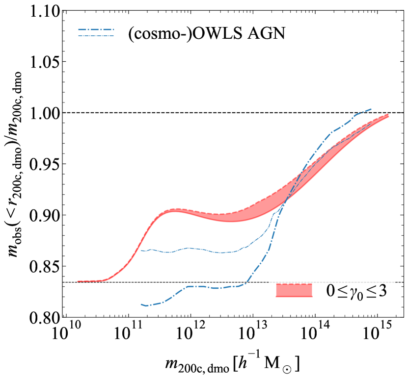
Figure 15: The ratio of the enclosed observed halo mass to the dark matter only equivalent mass at the fixed radius $r_{\mathrm{200c,dmo}}$ as a function of $m_{\mathrm{200c,dmo}}$. The shaded red region shows the spread in our models for all values of $\gamma_{0}$, i.e. the extrapolated power-law slope of the hot gas density profiles between $r_{\mathrm{500c,obs}}$ and $r_{\mathrm{200m,obs}}$, with red lines indicating $\gamma_{0}=0$ (red, dashed line) and $\gamma_{0}=3$ (red, solid line). The thin, black, dotted line indicates the ratio $1-f_{\mathrm{b}}$ that our model converges to when the halo baryon fraction reaches 0. The mass ratios at fixed radius $r_{\mathrm{200c,dmo}}$ converge towards high halo masses since not all values of $\gamma$ are allowed for massive haloes. For low masses, the ratios converge because the stellar component is held fixed and the gas fractions are low. The thick, blue, dash-dotted line shows the same relation at fixed radius $r_{\mathrm{200c,dmo}}$ in the (cosmo-)OWLS AGN simulation (Velliscig et al., 2014). The thin, blue, dash-dotted line shows the simulation relation corrected for changes in the dark matter mass profiles at $r_{\mathrm{200c,dmo}}$ with respect to the DMO equivalent haloes, since our model assumes that baryons do not affect the dark matter profile. The remaining difference in the mass ratio is due to differing baryon fractions between our model and the simulations.

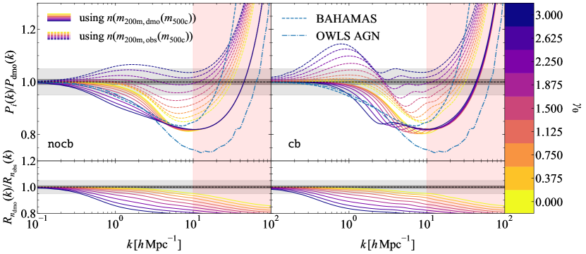
Figure 16: Top row The influence of correcting the halo abundance for the halo mass decrease due to baryonic processes. The dark and light gray bands indicate the $1\text{\,}\mathrm{\char 37\relax}$ and $5\text{\,}\mathrm{\char 37\relax}$ intervals. The left-hand panel shows model $\mathtt{nocb}$, which effectively assumes that the baryons missing from haloes are redistributed far beyond $r_{\mathrm{200m,obs}}$ on linear scales. The right-hand panel shows model $\mathtt{cb}$, which adds the missing halo baryons in a uniform profile outside but near $r_{\mathrm{200m,obs}}$. The red, lightly-shaded region for $k>$10\text{\,}$\mathrm{\mathit{h}}\,\mathrm{M}\mathrm{pc}^{-1}$$$ indicates the scales where our model is is not a good indicator of the uncertainty because the stellar component is not varied. The lines are colour-coded by $\gamma_{0}\equiv\gamma(m_{\mathrm{500c}}\to 0)$, the extrapolated power-law slope of the hot gas density profiles between $r_{\mathrm{500c,obs}}$ and $r_{\mathrm{200m,obs}}$, with lower values of $\gamma_{0}$ corresponding to flatter slopes. We show the power spectrum response with (our fiducial models, solid lines) and without (dashed lines) the correction for the halo masses applied. In the latter case, we find more power than in the DMO case at large scales because the abundance of low-mass haloes is overestimated due to not accounting for their mass loss compared to their DMO equivalents. Bottom row The ratio of the power spectrum with and without correction for the halo masses. Models with flatter slopes, i.e. lower values of $\gamma_{0}$, reach the cosmic baryon fraction at $r_{\mathrm{200m,obs}}$ for lower halo masses, resulting in the same total mass-abundance relation as the DMO equivalent halo for a larger range of halo masses and thus more similar power spectra.

Since halo abundances are generally obtained from N-body simulations, it is crucial that we are able to correctly link observed haloes to their dark matter only equivalents. However, astrophysical feedback processes result in the ejection of gas and, consequently, a modification of the halo profile and the halo mass $m_{\mathrm{200m}}$ (e.g. Sawala et al., 2013; Velliscig et al., 2014; Schaller et al., 2015). Thus, not accounting for the change in halo mass due to baryonic feedback would result in the wrong relation between halo density profiles and halo abundances in our model. Generally, feedback results in lower extrapolated halo masses $m_{\mathrm{200m,obs}}$ for the observed haloes than the DMO equivalent halo masses $m_{\mathrm{200m,dmo}}$. Thus, using the observed mass instead of the DMO equivalent mass in the halo mass function would result in an overprediction of the abundance of the observed halo since $n(m)$ decreases with increasing halo mass.

We described how we link $m_{\mathrm{200m,obs}}$ to $m_{\mathrm{200m,dmo}}$ in § 2.2. We remind the reader that we assume that baryons do not significantly alter the distribution of dark matter. Thus, the dark matter component of the observed halo has the same scale radius as its DMO equivalent and a mass that is a factor $1-\Omega_{\mathrm{b}}/\Omega_{\mathrm{m}}$ lower. The baryonic component of the observed halo is determined by the observations and our different extrapolations for $r>r_{\mathrm{500c,obs}}$. Then, from the total and rescaled DM density profiles of the observed halo, we can determine the masses $m_{\mathrm{200m,obs}}$ and $m_{\mathrm{200m,dmo}}$, respectively. These two masses will differ because the baryons do not follow the dark matter. The haloes have the abundance $n(m_{\mathrm{200m,dmo}}(m_{\mathrm{200m,obs}}))$ for which we use the halo mass function determined by Tinker et al. (2008). In this section, we test how this correction, i.e. using $n(m_{\mathrm{200m,dmo}}(m_{\mathrm{200m,obs}}))$ instead of $n(m_{\mathrm{200m,obs}})$, modifies our results.

We show the ratio of the observed halo mass to the DMO equivalent halo mass at fixed radius $r_{\mathrm{200c,dmo}}$ in Fig. 15. This ratio does not depend on the model type, i.e. $\mathtt{cb}$ or $\mathtt{nocb}$, since their density profiles are the same for $r<r_{\mathrm{200m,obs}}$. We indicate the range spanned by our models with $0\leq\gamma_{0}\leq 3$ by the red shaded region. They converge at the high-mass end because not all slopes $\gamma$ are allowed for high-mass haloes, as shown in § 4. At the low-mass end, our models converge because the stellar component is fixed and hence does not depend on $\gamma_{0}$, and the gas fractions approach 0. The thin, black, dotted line indicates the ratio $1-f_{\mathrm{b}}$ that our model converges to when the halo baryon fraction reaches 0.

We also show the same relation found in the OWLS AGN (low-mass haloes, Schaye et al., 2010) and cosmo-OWLS (high-mass haloes, Le Brun et al., 2014) simulations from Velliscig et al. (2014). There are systematic differences between the predictions from the simulations and our model. These differences occur for two reasons. First, our assumption that the baryons do not alter the distribution of the dark matter with respect to the DMO equivalent halo, does not hold in detail. Velliscig et al. (2014) show that at the fixed radius $r_{\mathrm{200c,dmo}}$ there is a difference of up to $4\text{\,}\mathrm{\char 37\relax}$ between the dark matter mass of the observed halo and the dark matter mass of the DMO equivalent halo, rescaled to account for the cosmic baryon fraction. The dark matter in low-mass haloes expands due to feedback expelling baryons outside $r_{\mathrm{200c,dmo}}$. In the highest-mass haloes, feedback is less efficient and the dark matter contracts in response to the cooling baryons. The thin, blue, dash-dotted line shows the relation in OWLS AGN when forcing the dark matter mass of the halo to equal the rescaled DMO equivalent halo mass. Hence, the contraction due to the presence of baryons of the dark matter component for high-mass haloes explains the difference between our model and the simulations. For the low-mass end, the expansion of the dark matter component is not sufficient to explain all of the difference. The remaining discrepancy results from the higher baryons fractions in our model compared to the simulations.

We will neglect the response of the DM to the redistribution of baryons throughout the rest of the paper. We have checked that scaling the halo density profiles of the DMO equivalent haloes to match the mass ratios from the OWLS AGN simulation only affects our predictions of the power suppression at the $\approx$1\text{\,}\mathrm{\char 37\relax}$$ level at our scales of interest (i.e. $k<$10\text{\,}$\mathrm{\mathit{h}}\,\mathrm{M}\mathrm{pc}^{-1}$$$). However, even this small correction is an upper limit because we have assumed a fixed ratio between the DM and rescaled DMO density profiles that exceeds the correction for the cosmic baryon fraction. Hence, even at large distances $r\gg r_{\mathrm{200c,dmo}}$ the mass ratio between the halo and its DMO equivalent does not converge, whereas the mass difference between hydrodynamical haloes and their DMO equivalents eventually decreases to 0 (see e.g. Velliscig et al., 2014; van Daalen et al., 2014). We find such a small effect because the low-mass haloes, whose mass ratio differs the most between our model and the OWLS AGN simulation, only have a small effect on the total power at large scales, as we will show in § 5.3.

We show how the correction of the halo abundance for the change in halo mass due to baryonic processes affects the predicted power spectrum response to baryons in Fig. 16. In the top row, we show the power spectrum response for both the $\mathtt{nocb}$ (left panel) and $\mathtt{cb}$ models (right panel) with (our fiducial models, solid lines) and without (dashed lines) the halo mass correction. When not correcting the halo abundance for the change in halo mass (i.e. when using $n(m_{\mathrm{200m,obs}})$), we actually find an increase in power with respect to the DMO model at scales $k\lesssim$1\text{\,}$\mathrm{\mathit{h}}\,\mathrm{M}\mathrm{pc}^{-1}$$$, i.e. $R_{i}(k)>1$, for both the $\mathtt{nocb}$ and $\mathtt{cb}$ models, since the inferred abundances for observed haloes with masses $m_{\mathrm{200m,obs}}\lesssim${10}^{14}\text{\,}$\mathrm{\mathit{h}}^{-1}\,$Msun{\mathrm{M_{\odot}}}$$$$ are too high. At these scales, the Fourier profiles become constant in the 1h term, i.e. $\hat{\rho}(k|m_{\mathrm{h}})\to m_{\mathrm{h}}$ in Eq. 4, and the power spectrum behaviour is thus dictated entirely by the halo abundance. Hence, the power suppression that we find in our fiducial models at these scales is the consequence of correcting the DMO equivalent halo masses to account for the ejection of matter due to feedback. We stress that our implementation of this effect is purely empirical and does not rely on any assumptions about the physics involved in baryonic feedback processes.

In the bottom row of Fig. 16, we show the ratio between the power spectrum response to the inclusion of baryons with and without the DMO equivalent halo mass correction. The correction is most significant for the steepest extrapolated density profile slopes, i.e. the highest values of $\gamma_{0}$, for which we see the smallest ratios. For $\gamma_{0}=3$, even the most massive haloes do not reach the cosmic baryon fraction inside $r_{\mathrm{200m,obs}}$ (see Fig. 9), and, hence, even their abundances would be calculated wrongly if the observed total mass was used, instead of the rescaled, observed DM mass, to compute the halo abundance. In the case of the $\mathtt{cb}$ models, there is an extra increase in power for scales $k\lesssim$1\text{\,}$\mathrm{\mathit{h}}\,\mathrm{M}\mathrm{pc}^{-1}$$$ due to the more extended baryon distribution.

It is striking how the halo mass correction modifies the suppression of power in the way required to encompass the simulation predictions at large scales. The correction to the DMO equivalent halo masses is necessary for this match.

5.3 Contribution of different halo masses

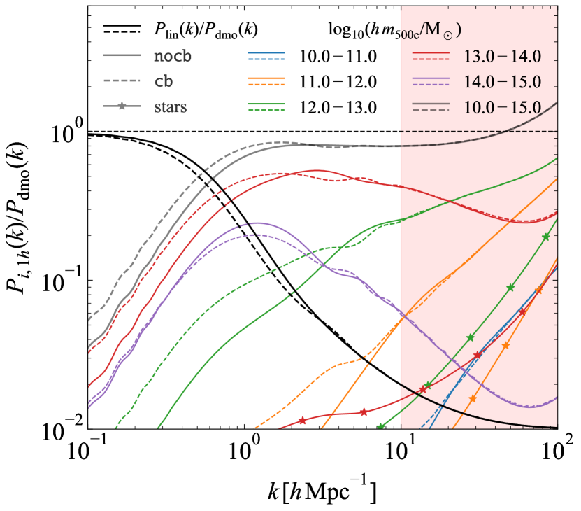
Figure 17: The contribution of the 1-halo term for different halo mass ranges to the total power spectrum at all scales for our fiducial models. The $\mathtt{nocb}$ (solid lines) and $\mathtt{cb}$ (dashed lines) models are shown and the mass ranges are indicated by the colours. We also show the contribution of the 2-halo term, i.e. the linear power spectrum (black lines). The stellar contribution (1h term and all cross-correlations between matter and stars, connected stars) is also included, but only for the $\mathtt{nocb}$ case, since the $\mathtt{cb}$ case traces the $\mathtt{nocb}$ lines. The red, lightly-shaded region for $k>$10\text{\,}$\mathrm{\mathit{h}}\,\mathrm{M}\mathrm{pc}^{-1}$$$ indicates the scales where our model is is not a good indicator of the uncertainty because the stellar component is not varied. The 1h term dominates the total power for $k\gtrsim$0.5\text{\,}$\mathrm{\mathit{h}}\,\mathrm{M}\mathrm{pc}^{-1}$$$. For the scales of interest here ($k\lesssim$5\text{\,}$\mathrm{\mathit{h}}\,\mathrm{M}\mathrm{pc}^{-1}$$$), most of the power is contributed by groups and clusters with $${10}^{13}\text{\,}$\mathrm{\mathit{h}}^{-1}\,$Msun{\mathrm{M_{\odot}}}$$$\leq m_{\mathrm{500c,obs}}\leq${10}^{15}\text{\,}$\mathrm{\mathit{h}}^{-1}\,$Msun{\mathrm{M_{\odot}}}$$$$. For the $\mathtt{cb}$ models, low-mass ($\approx${10}^{13}\text{\,}$\mathrm{\mathit{h}}^{-1}\,$Msun{\mathrm{M_{\odot}}}$$$$) haloes contribute more and clusters ($>${10}^{14}\text{\,}$\mathrm{\mathit{h}}^{-1}\,$Msun{\mathrm{M_{\odot}}}$$$$) less compared with the $\mathtt{nocb}$ models. The total stellar contribution to the power response is $\lesssim$1\text{\,}\mathrm{\char 37\relax}$$ for all scales $k\lesssim$5\text{\,}$\mathrm{\mathit{h}}\,\mathrm{M}\mathrm{pc}^{-1}$$$ and only exceeds $2\text{\,}\mathrm{\char 37\relax}$ for $k\gtrsim$10\text{\,}$\mathrm{\mathit{h}}\,\mathrm{M}\mathrm{pc}^{-1}$$$.

To determine the observables that best constrain the matter power spectrum at different scales, it is important to know which haloes dominate the suppression of power at those scales. The dominant haloes will be determined by the interplay between the total mass of the halo and its abundance.

The halo model linearly adds the contributions from haloes of all masses to the power at each scale. We show the contributions for five decades in mass in Fig. 17 for our fiducial model in the $\mathtt{nocb}$ and $\mathtt{cb}$ cases. We integrate the 1-halo term, Eq. 4, over 5 different decades in mass, spanning $${10}^{10}\text{\,}$\mathrm{\mathit{h}}^{-1}\,$Msun{\mathrm{M_{\odot}}}$$$<m_{\mathrm{500c,obs}}<${10}^{15}\text{\,}$\mathrm{\mathit{h}}^{-1}\,$Msun{\mathrm{M_{\odot}}}$$$$, and then divide each by the DMO power spectrum, showing the contribution of different halo masses to the power spectrum. We also show the contribution of the 2-halo term, i.e. the linear power spectrum. The mass dependence of our model comes entirely from the 1h term, which dominates the total power for $k\gtrsim$0.5\text{\,}$\mathrm{\mathit{h}}\,\mathrm{M}\mathrm{pc}^{-1}$$$.

We want to quantify the stellar contribution to the power spectrum to gauge whether we are allowed to neglect the ISM component of the gas. As explained in the beginning of § 2.3, we can safely neglect the ISM if the stellar component contributes negligibly to the total power at our scales of interest ($k\lesssim$5\text{\,}$\mathrm{\mathit{h}}\,\mathrm{M}\mathrm{pc}^{-1}$$$). To this end, we also include the 1h term for the stellar component with all cross-correlations $|\rho_{\star}(k|m_{\mathrm{h}})\rho_{i}(k|m_{\mathrm{h}})|$ in Eq. (4) with $i\in\{\mathrm{dm,gas}\}$. We only show this contribution for the $\mathtt{nocb}$ case, since the $\mathtt{cb}$ results are nearly identical. Fig. 17 clearly shows that the stellar component contributes negligibly to the power for all scales $k\lesssim$5\text{\,}$\mathrm{\mathit{h}}\,\mathrm{M}\mathrm{pc}^{-1}$$$ and, hence, we are justified in neglecting the contributions of the ISM to the gas component. However, for making predictions at the $1\text{\,}\mathrm{\char 37\relax}$ level on small scales ($k\gtrsim$5\text{\,}$\mathrm{\mathit{h}}\,\mathrm{M}\mathrm{pc}^{-1}$$$), the ISM and stellar components will become important and will need to be modelled more accurately.

At all scales $k\lesssim$10\text{\,}$\mathrm{\mathit{h}}\,\mathrm{M}\mathrm{pc}^{-1}$$$, the total power is dominated by groups ($${10}^{13}\text{\,}$\mathrm{\mathit{h}}^{-1}\,$Msun{\mathrm{M_{\odot}}}$$$\leq m_{\mathrm{500c,obs}}\leq${10}^{14}\text{\,}$\mathrm{\mathit{h}}^{-1}\,$Msun{\mathrm{M_{\odot}}}$$$$) and clusters ($${10}^{14}\text{\,}$\mathrm{\mathit{h}}^{-1}\,$Msun{\mathrm{M_{\odot}}}$$$\leq m_{\mathrm{500c,obs}}\leq${10}^{15}\text{\,}$\mathrm{\mathit{h}}^{-1}\,$Msun{\mathrm{M_{\odot}}}$$$$) of galaxies, with groups providing a similar or greater contribution than clusters. Similar results have been found in DMO simulations by van Daalen & Schaye (2015). Group-mass haloes have the largest range in possible baryon fractions in our model, depending on the slope $\gamma_{0}$ of the gas density profile for $r>r_{\mathrm{500c,obs}}$. We conclude that groups are crucial contributors to the power at large scales and thus measuring the baryon content of group-mass haloes will provide the main observational constraint on predictions of the baryonic suppression of the matter power spectrum.

5.4 Influence of density profile fitting parameters

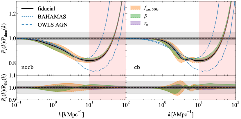
Figure 18: Top row The variation in the power suppression due to baryonic effects when varying the best-fit hot gas density profile parameters independently within their $15^{\mathrm{th}}$ (dashed lines) and $85^{\mathrm{th}}$ (solid lines) percentile ranges (shaded regions) and keeping all other parameters fixed. The dark and light gray bands indicate the $1\text{\,}\mathrm{\char 37\relax}$ and $5\text{\,}\mathrm{\char 37\relax}$ intervals. The left-hand panel shows model $\mathtt{nocb}$, which effectively assumes that the baryons missing from haloes are redistributed far beyond $r_{\mathrm{200m,obs}}$ on linear scales. The right-hand panel shows model $\mathtt{cb}$, which adds the missing halo baryons in a uniform profile outside but near $r_{\mathrm{200m,obs}}$. The red, lightly-shaded region for $k>$10\text{\,}$\mathrm{\mathit{h}}\,\mathrm{M}\mathrm{pc}^{-1}$$$ indicates the scales where our model is is not a good indicator of the uncertainty because the stellar component is not varied. The thick, solid, black line indicates our fiducial model with $\gamma_{0}=3\beta=2.14$. Bottom row The ratio between the region enclosed by the $15^{\mathrm{th}}-85^{\mathrm{th}}$ percentiles for each fit parameter and the fiducial model. The parameters $\beta$ and $f_{\mathrm{gas,500c}}$ determine the behaviour in the outer regions and are most important. The same trends are present for both the $\mathtt{nocb}$ and $\mathtt{cb}$ cases, but the $\mathtt{nocb}$ case is sensitive to variations in the best-fit parameters out to larger scales. The uncertainty in any of the best-fit parameters allows at most a $\pm$5\text{\,}\mathrm{\char 37\relax}$$ variation in the power suppression for any scale.

So far, we have shown the impact of the baryon distribution and haloes of different masses on the matter power spectrum for different wavenumbers when assuming our model that best fits the observations. However, since we assume the median values for the parameters $r_{\mathrm{c}}$ and $\beta$, and the median relation $f_{\mathrm{gas,500c}}-m_{\mathrm{500c,obs}}$ for the observed hot gas density profiles and there is a significant scatter around these medians, it is important to see how sensitive our predictions are to variations in the parameter values. In this section, we investigate the isolated effect of each observational parameter on the predicted matter power spectrum.

We remind the reader of the beta profile in Eq. 14 and the best fits for its parameters determined from the observations in Figs. 2, 5, and 6. In those figures, we indicated the median relations, which are used in our model, and the $15^{\mathrm{th}}$ and $85^{\mathrm{th}}$ percentiles of the observed values. We will test the model response to variations in the hot gas observations by varying each of the best-fit parameters between its $15^{\mathrm{th}}$ and $85^{\mathrm{th}}$ percentiles while keeping all other parameters fixed.

We show the result of these parameter variations for our fiducial model ($\gamma_{0}=2.14$) in the $\mathtt{nocb}$ and $\mathtt{cb}$ cases in Fig. 18. We indicate the $15^{\mathrm{th}}$ ($85^{\mathrm{th}}$) percentile envelope with a dashed (solid), coloured line and shade the region enclosed by these percentiles. For both the $\mathtt{cb}$ and $\mathtt{nocb}$ cases, the parameters $\beta$ and $f_{\mathrm{gas,500c}}$ are the most important at large scales. Flatter outer slopes for the hot gas density profile, i.e. smaller values of $\beta$, will result in more baryons out to $r_{\mathrm{200m,obs}}$, yielding a smaller suppression of power on large scales. Higher gas fractions within $r_{\mathrm{500c,obs}}$ will result in haloes that are more massive and contain more of the baryons, again yielding a smaller suppression of power on large scales. The core radius $r_{\mathrm{c}}$ is the least important parameter. Increasing the size of the core requires a lower density in the core to reach the same gas fraction at $r_{\mathrm{500c,obs}}$ and yields more baryons in the halo outskirts. Hence, we see more power at large scales and less power on small scales when increasing the value of $r_{\mathrm{c}}$ similarly to decreasing the value $\beta$. However, the core is relatively close to the cluster center and thus has no impact on the matter distribution at large scales.

There is an important difference between the $\mathtt{nocb}$ and $\mathtt{cb}$ cases, however. The fit parameters only start having an effect on the power suppression at scales $k\gtrsim$1\text{\,}$\mathrm{\mathit{h}}\,\mathrm{M}\mathrm{pc}^{-1}$$$ in the $\mathtt{cb}$ case, whereas in the $\mathtt{nocb}$ case they already start mattering around $k\approx$0.3\text{\,}$\mathrm{\mathit{h}}\,\mathrm{M}\mathrm{pc}^{-1}$$$. If all baryons are accounted for in the halo outskirts, as in the $\mathtt{cb}$ case, the details of the baryon distribution do not matter for the power at the largest scales, since here the 1h term is fully determined by the mass inside $r_{\mathrm{h}}$, which does not change for different values of $\beta$ and $f_{\mathrm{gas,500c}}$. The $\mathtt{nocb}$ model is a lot more sensitive to the baryon distribution within the halo, since depending on the value of $\beta$, or how many baryons can already be accounted for inside $r_{\mathrm{500c,obs}}$, the haloes can have large variations in mass $m_{\mathrm{200m,obs}}$.

In conclusion, the most important parameter to pin down is the gas fraction of the halo, as we already concluded in § 5.1 and § 5.3. It has the largest effect on all scales in both the $\mathtt{nocb}$ and $\mathtt{cb}$ cases and varying its value within the observed scatter results in a $\approx\pm$5\text{\,}\mathrm{\char 37\relax}$$ variation around the power spectrum response predicted by our fiducial model. At the scales of interest to future surveys, the effect of $\beta$ is of similar amplitude. However, this parameter will be harder to constrain observationally than the gas content of the halo, especially for group-mass haloes, because X-ray observations cannot provide an unbiased sample and SZ observations cannot observe the density profile directly.

5.5 Influence of hydrostatic bias

Figure 19: Top row The response of the matter power spectrum to the presence of baryons with (dashed lines) and without (solid lines) accounting for a hydrostatic bias of $1-b=0.7$ in the halo mass. The dark and light gray bands indicate the $1\text{\,}\mathrm{\char 37\relax}$ and $5\text{\,}\mathrm{\char 37\relax}$ intervals. The left-hand panel shows model $\mathtt{nocb}$, which effectively assumes that the baryons missing from haloes are redistributed far beyond $r_{\mathrm{200m,obs}}$ on linear scales. The right-hand panel shows model $\mathtt{cb}$, which adds the missing halo baryons in a uniform profile outside but near $r_{\mathrm{200m,obs}}$. The red, lightly-shaded region for $k>$10\text{\,}$\mathrm{\mathit{h}}\,\mathrm{M}\mathrm{pc}^{-1}$$$ indicates the scales where our model is is not a good indicator of the uncertainty because the stellar component is not varied. Bottom row The ratio between the corrected and the uncorrected models. Haloes with lower values of $\gamma_{0}$ are less strongly affected by the bias since they can add more baryons outside $r_{\mathrm{500c,obs}}$. Without correcting for the bias, we underestimate the suppression of power by up to $\approx$4\text{\,}\mathrm{\char 37\relax}$$ at $k=$1\text{\,}$\mathrm{\mathit{h}}\,\mathrm{M}\mathrm{pc}^{-1}$$$.

All of our results so far assumed gas fractions based on halo masses derived from X-ray observations under the assumption of hydrostatic equilibrium (HE) and pure thermal pressure. Under the HE assumption non-thermal pressure and large-scale gas motions are neglected in the Euler equation (see e.g. the discussion in §2.3 of Pratt et al., 2019). However, in massive systems in the process of assembly, there is no a priori reason to assume that simplifying assumption to hold. We expect the most massive clusters to depart from HE, since we know from the hierarchical structure formation paradigm, that they have only recently formed. Moreover, the pressure can have a non-negligible contribution from non-thermal sources such as turbulence (Eckert et al., 2019).

Investigating the relation between hydrostatically derived halo masses and the true halo mass requires hydrodynamical simulations (e.g. Nagai et al., 2007; Rasia et al., 2012; Biffi et al., 2016; Le Brun et al., 2017; McCarthy et al., 2017; Henson et al., 2017) or weak gravitational lensing observations (Mahdavi et al., 2013; Von der Linden et al., 2014; Hoekstra et al., 2015; Medezinski et al., 2018). In both cases, the pressure profile of the halo is derived from observations of the hot gas. Under the assumption of spherical symmetry and HE, this pressure profile is then straightforwardly related to the total mass profile of the halo. Subsequently, this hydrostatic halo mass can be compared to an unbiased estimate of the halo mass, i.e. the true mass in hydrodynamical simulations, or the mass derived from weak lensing observations.

The picture arising from both simulations and observations is that hydrostatic masses, $m_{\mathrm{HE}}$, are generally biased low with respect to the weak lensing or true halo mass, $m_{\mathrm{WL}}$, with $m_{\mathrm{HE}}/m_{\mathrm{WL}}=1-b\simeq$0.60.9$$ (e.g. Mahdavi et al., 2013; Von der Linden et al., 2014; Hoekstra et al., 2015; Le Brun et al., 2017; Henson et al., 2017; Medezinski et al., 2018). The detailed behaviour of this bias depends on the deprojected temperature and density profiles, with more spherical systems being less biased.

Correcting for the observationally determined bias would result in higher halo masses and, consequently, a shift in the gas fractions away from the assumed best-fit $f_{\mathrm{gas,500c}}-m_{\mathrm{500c,obs}}$ relation. We argued previously that this is the most relevant observable to determine the suppression of power at scales $k\lesssim$1\text{\,}$\mathrm{\mathit{h}}\,\mathrm{M}\mathrm{pc}^{-1}$$$. Thus, it is important to investigate how the HE assumption affects our predictions. Previously, Schneider et al. (2019) have shown for three different levels of hydrostatic bias ($1-b\in\{0.71,0.83,1\}$) that the predicted power suppression at large scales $k<$1\text{\,}$\mathrm{\mathit{h}}\,\mathrm{M}\mathrm{pc}^{-1}$$$ can vary by up to $5\text{\,}\mathrm{\char 37\relax}$.

Staying in tune with § 5.4, we adopt a single value for the bias to investigate its influence on our predictions. We will take $1-b=0.7$ which is consistent with both Von der Linden et al. (2014) and Hoekstra et al. (2015). Moreover, although the bias tends to be higher for higher-mass systems because of the presence of cooler gas in their outskirts (Henson et al., 2017), we conservatively adopt this value for all halo masses. Correcting for the bias will influence our model in two ways. First, the inferred gas masses will increase slightly, since the true $r_{\mathrm{500c,obs}}$ will be larger than the value assumed from the hydrostatic estimate. We thus recompute the gas masses from our best-fit beta models to the observations. Second, the halo mass will increase by the bias factor which will result in new estimates for the gas fractions, which we show as the thin, solid, black line in Fig. 2. We then fit the median $f_{\mathrm{gas,500c}}-m_{\mathrm{500c,obs}}$ relation again, assuming Eq. 25, resulting in the thin, red, dashed line.

We show the resulting effect on the baryonic suppression of the power spectra in Fig. 19. The results are similar to varying $f_{\mathrm{gas,500c}}$ in Fig. 18, since the bias-corrected relation is similar to the 15^th percentile $f_{\mathrm{gas,500c}}-m_{\mathrm{500c,obs}}$ relation, but with a more dramatic suppression of the baryonic mass for clusters and hence more suppression of the power at large scales. In the bottom panels of Fig. 19, we find a maximum extra suppression of $\approx$4\text{\,}\mathrm{\char 37\relax}$$ due to the hydrostatic bias at $k=$1\text{\,}$\mathrm{\mathit{h}}\,\mathrm{M}\mathrm{pc}^{-1}$$$ in both the $\mathtt{nocb}$ and $\mathtt{cb}$ cases, which is consistent with the findings of Schneider et al. (2019). The magnitude of the suppression is lower for lower values of $\gamma_{0}$ since these models compensate for the lower baryon fraction within $r_{\mathrm{500c,obs}}$ by adding baryons between $r_{\mathrm{500c,obs}}$ and $r_{\mathrm{h}}$.

Accounting for the bias breaks the overall agreement with the simulations on large scales for the models with high values of $\gamma_{0}$. However, in bahamas and OWLS AGN, a hydrostatic bias of $1-b=0.84$ and $1-b=0.8$ is found, respectively, for groups and clusters (McCarthy et al., 2017; Le Brun et al., 2014). When we assume $1-b=0.8$, we find a maximum extra suppression of $\approx$2\text{\,}\mathrm{\char 37\relax}$$ at $k=$1\text{\,}$\mathrm{\mathit{h}}\,\mathrm{M}\mathrm{pc}^{-1}$$$ instead of $\approx$4\text{\,}\mathrm{\char 37\relax}$$. At other scales the effect of the hydrostatic bias is similarly reduced.

In conclusion, it is crucial to obtain robust constraints on the hydrostatic bias of groups and clusters of galaxies. Current measurements of this bias suggest that hydrostatic halo masses underestimate the true masses and that this bias results in a downward shift of the cluster gas fractions that is more severe than the observational scatter in the relation. Because the shift affects cluster-mass haloes, it results in an additional power suppression of up to $\approx$4\text{\,}\mathrm{\char 37\relax}$$ at $k=$1\text{\,}$\mathrm{\mathit{h}}\,\mathrm{M}\mathrm{pc}^{-1}$$$, depending on how our model distributes the outer baryons. There are ways of measuring halo masses that do not rely on making the hydrostatic assumption, such as weak lensing observations, but these also carry their own intrinsic biases (Henson et al., 2017). Making mock observations in simulations allows us to characterize these separate biases (e.g. Henson et al., 2017; Le Brun et al., 2017), but the simulations still do not make a full like-for-like comparison with the observations. Finally, joint constraints on X-ray, SZ, and weak lensing halo mass scaling relations, including possible biases, as was done in Bocquet et al. (2019), could provide more robust halo mass estimates.

6 Discussion

We have presented an observationally constrained halo model to estimate the power suppression due to baryons without any reliance on subgrid recipes for the unresolved physics of baryons in hydrodynamical simulations. We reiterate that our main goal is not to provide the most accurate predictions of the matter power spectrum, but to investigate the possibility of using observations to constrain it. The fact that the clustering of matched haloes does not change between DMO and hydrodynamical simulations (van Daalen et al., 2014) implies that changes in the density profiles due to the baryons determine the change of the matter power spectrum. Hence, even though the halo model does not accurately predict the matter power spectrum, it can accurately predict the relative effect of baryonic processes on the power spectrum. The overall agreement between our model and hydrodynamical simulations that reproduce the observed distribution of baryons in groups and clusters, confirms that our model captures the first-order impact of baryons simply by reproducing the observed baryon content for groups and clusters.

In conclusion, the main strength of the model is that it allows us to quantify the impact of different halo masses, different halo baryon density distributions and observational biases and uncertainties on the baryonic suppression of the matter power spectrum without any necessity for uncertain subgrid recipes for feedback processes. This in turn allows us to provide a less model-dependent estimate of the range of possible baryonic suppression and to predict which observations would provide the strongest constraints on the matter power spectrum.

There are other models in the literature that aim to model the effect of baryon physics on the matter power spectrum. HMcode by Mead et al. (2015) is widely used to include baryon effects in weak lensing analyses. Although HMcode is also based on the halo model, its aim is different from ours. Mead et al. (2015) modify the dark matter halo profiles and subsequently fit the parameters of their halo model to hydrodynamical simulations to provide predictions for the baryonic response of the power spectrum that are accurate at the $\sim$5\text{\,}\mathrm{\char 37\relax}$$ level for $k\lesssim$5\text{\,}$\mathrm{\mathit{h}}\,\mathrm{M}\mathrm{pc}^{-1}$$$ with 2 free parameters related to the baryonic feedback (for a similar approach, see Semboloni et al., 2013). These feedback parameters can then be jointly constrained with the cosmology using cosmic shear data. However, even though the modifications to the dark matter profile are phenomenologically inspired, there is no guarantee that the final best-fit parameters correspond to the actual physical state of the haloes. We obtain similar accuracy in the predicted power response when viewing $\gamma_{0}$ as a fitting parameter and comparing to hydrodynamical simulations. However, in our case, fitting $\gamma_{0}$ preserves the agreement with observations. Indeed, the most important difference between our approach and that of Mead et al. (2015) is that we fit to observations instead of simulations.

The investigation of Schneider et al. (2019) most closely matches our goal. Schneider & Teyssier (2015) and Schneider et al. (2019) developed a baryon correction model to investigate the influence of baryon physics on the matter power spectrum. Their model shifts particles in DMO simulations according to the physical expectations from baryonic feedback processes. Since the model only relies on DMO simulations, it is not as computationally expensive as models that require hydrodynamical simulations to calibrate their predictions. Our simple analytic halo model is cheaper still to run, but it only results in a statistical description of the matter distribution, whereas the baryon correction model predicts the total matter density field for the particular realization that was simulated. Because our model combines the universal DMO halo mass function with observed density profiles, it can easily be applied to a wide variety of cosmologies without having to run an expensive grid of DMO simulations.

In the baryon correction model, the link to observations can also be made, making it similar to our approach. Schneider et al. (2019) fit a mass-dependent slope of the gas profile, $\beta$ (note that their slope is not defined the same way as our slope $\beta$), and the maximum gas ejection radius, $\theta_{\mathrm{ej}}$, to the observed hot gas profiles of the XXL sample of Eckert et al. (2016) and a compendium of X-ray gas fraction measurements. They also include a stellar component that is fit to abundance matching results, similar to our iHOD implementation. They show that their model can reproduce the observed relations as well as hydrodynamical simulations when fit to their gas fractions. Schneider et al. (2019) use the observations to set a maximum range on their model parameters to then predict both the matter power spectrum and the shear correlation function. Our work, on the other hand, focusses on the impact of isolated properties of the baryon distribution on the power spectrum. Similarly to Schneider et al. (2019), we find that the power suppression on large scales is very sensitive to the baryon distribution in the outskirts of the halo. However, our model allows us to clearly show that the halo baryon fractions are the crucial ingredient in setting the total power suppression at large scales, $k\lesssim$1\text{\,}$\mathrm{\mathit{h}}\,\mathrm{M}\mathrm{pc}^{-1}$$$. Also similarly to Schneider et al. (2019), we find that the hydrostatic mass bias significantly affects the total power suppression at large scales.

So far, we have not included redshift evolution. Schneider et al. (2019) have found that the most important evolution of clusters and groups in cosmological simulations stems from the change in their abundance due to the evolution of the halo mass function in time, and not due to the change of the density profiles with time. This evolution can be readily implemented into our halo model.

7 Summary and conclusions

Future weak lensing surveys will be limited in their accuracy by how well we can predict the matter power spectrum on small scales (e.g. Semboloni et al., 2011; Copeland et al., 2018; Huang et al., 2019). These scales contain a wealth of information about the underlying cosmology of our Universe, but the interpretation of the signal is complicated by baryon effects. Our current theoretical understanding of the impact of baryons on the matter power spectrum stems from hydrodynamical simulations that employ uncertain subgrid recipes to model astrophysical feedback processes. This uncertainty can be bypassed by adopting an observational approach to link the observed distribution of matter to the matter power spectrum.

We have provided a detailed study of the constraints that current observations of groups and clusters of galaxies impose on the possible influence of the baryon distribution on the matter power spectrum. We introduced a modified halo model that includes dark matter, hot gas, and stellar components. We fit the hot gas to X-ray observations of clusters of galaxies and we assumed different distributions for the missing baryons outside $r_{\mathrm{500c,obs}}$, the maximum radius probed by X-ray observations of the hot gas distribution. Subsequently, we quantified (i) how the outer, unobserved baryon distribution modifies the matter power spectrum (Fig. 11). We also investigated (ii) how the change in halo mass due to baryonic effects can be incorporated into the halo model (Fig. 16). We showed (iii) the contributions to the matter power spectrum of haloes of different masses at different spatial scales (Fig. 17), (iv) the influence of varying the individual best-fit parameters to the observed density profiles within their allowed range (Fig. 18), and (v) the influence of a hydrostatic mass bias on the matter power spectrum (Fig. 19).

Our model has one free parameter, $\gamma_{0}$, related to the slope of the hot gas density profile for $r_{\mathrm{500c,obs}}\leq r\leq r_{\mathrm{200m,obs}}$, where observational constraints are very poor. We considered two extreme cases for the baryons. First, the $\mathtt{nocb}$ models assume that haloes of size $r_{\mathrm{200m,obs}}$ do not necessarily reach the cosmic baryon fraction at this radius and that any missing baryons are located at such large distances that they only contribute to the 2-halo term. Second, in the $\mathtt{cb}$ models the missing baryons inside $r_{\mathrm{200m,obs}}$ are distributed with an assumed uniform density profile outside this radius until the cosmic baryon fraction is reached. These cases provide, respectively, the maximum and minimum power suppression of large-scale power due to baryonic effects.

All of our observationally constrained models predict a significant amount of suppression on the scales of interest to future surveys ($$0.2$\lesssim k/($$\mathrm{\mathit{h}}\,\mathrm{M}\mathrm{pc}^{-1}$$)\lesssim$5$$). We find a total suppression of $1\text{\,}\mathrm{\char 37\relax}$ ($5\text{\,}\mathrm{\char 37\relax}$) on scales $0.20.9\text{\,}$\mathrm{\mathit{h}}\,\mathrm{M}\mathrm{pc}^{-1}$$ ($0.52\text{\,}$\mathrm{\mathit{h}}\,\mathrm{M}\mathrm{pc}^{-1}$$) in the $\mathtt{nocb}$ case and on scales $0.51\text{\,}$\mathrm{\mathit{h}}\,\mathrm{M}\mathrm{pc}^{-1}$$ ($12\text{\,}$\mathrm{\mathit{h}}\,\mathrm{M}\mathrm{pc}^{-1}$$) in the $\mathtt{cb}$ case for values $\gamma_{0}=$30$$ (Fig. 11), where $\gamma_{0}$ is the low-mass limit of the power-law slope $\gamma$ between $r_{\mathrm{500c,obs}}$ and $r_{\mathrm{200m,obs}}$, i.e. $\gamma_{0}=\gamma(m_{\mathrm{500c,obs}}\to 0)$. This large possible range of scales corresponding to a fixed suppression factor for each case illustrates the importance of the baryon distribution outside $r_{\mathrm{500c,obs}}$ (which is parameterised by $\gamma_{0}$) in setting the total power suppression.

We found that massive groups of galaxies ($${10}^{13}\text{\,}$\mathrm{\mathit{h}}^{-1}\,$Msun{\mathrm{M_{\odot}}}$$$<m_{\mathrm{500c,obs}}<${10}^{14}\text{\,}$\mathrm{\mathit{h}}^{-1}\,$Msun{\mathrm{M_{\odot}}}$$$$) provide a larger contribution than clusters to the total power at all scales (Fig. 17). This is unfortunate, since we have shown that the baryonic content of group- and cluster-sized haloes, which is set by the observed gas fractions $f_{\mathrm{gas,500c}}$, determines the large-scale ($k\lesssim$1\text{\,}$\mathrm{\mathit{h}}\,\mathrm{M}\mathrm{pc}^{-1}$$$) power suppression (Figs. 14 and 18). However, observations of the hot gas content of groups are scarcer than those of clusters and are also subject to a considerable Malmquist bias. Current X-ray telescopes cannot solve this problem, but a combined approach with Sunyaev-Zel’dovich or gravitational lensing observations could provide a larger sample of lower mass objects.

We found that our observationally constrained models only encompass the predictions of hydrodynamical simulations that reproduce the hot gas content of groups and clusters of galaxies (Fig. 12). Thus, we stress the importance of using simulations that reproduce the relevant observations when using such models to predict the baryonic effects on the matter distribution.

We found that accurately measuring the halo masses is of vital importance when trying to place observational constraints on the matter power spectrum. An unrecognized hydrostatic halo mass bias of $1-b=0.7$ would result in an underestimate of the total power suppression by as much as $4\text{\,}\mathrm{\char 37\relax}$ at $k=$1\text{\,}$\mathrm{\mathit{h}}\,\mathrm{M}\mathrm{pc}^{-1}$$$ (Fig. 19). In addition, it is critical to correct the observed halo masses for the redistribution of baryons when estimating their abundance using halo mass functions based on DM only simulations (Fig. 16).

All in all, it is encouraging that we are able to quantify the baryonic suppression of the matter power spectrum with a simple, flexible but physical approach such as our modified halo model. Our investigation allows us to predict the observations that will be most constraining for the impact of baryonic effects on the matter power spectrum.

Appendix A Influence of the halo mass range

In this section, we investigate how our choice of mass grid influences our predictions. We have chosen an equidistant log-grid of halo masses $${10}^{11}\text{\,}$\mathrm{\mathit{h}}^{-1}\,$Msun{\mathrm{M_{\odot}}}$$$\leq m_{\mathrm{500c,obs}}\leq${10}^{15}\text{\,}$\mathrm{\mathit{h}}^{-1}\,$Msun{\mathrm{M_{\odot}}}$$$$, sampled with 101 bins. Doubling or halving the number of bins only affects our predictions at the $<$0.1\text{\,}\mathrm{\char 37\relax}$$ level for all $k$. Similarly, increasing the maximum halo mass to $m_{\mathrm{500c,max}}=${10}^{16}\text{\,}$\mathrm{\mathit{h}}^{-1}\,$Msun{\mathrm{M_{\odot}}}$$$$ only results in changes at the $<$0.1\text{\,}\mathrm{\char 37\relax}$$ level for all $k$. The only significant change occurs when decreasing the minimum halo mass to $m_{\mathrm{500c,min}}=${10}^{6}\text{\,}$\mathrm{\mathit{h}}^{-1}\,$Msun{\mathrm{M_{\odot}}}$$$$, but this only affects scales smaller than of interest here. In this case, our baryonic models predict less power compared to the higher minimum mass case, since the low-mass haloes have no stars and gas. Hence, they will always contain less matter than their DMO equivalents and the DMO power will be boosted relative to the baryonic one. However, our predictions only change at the $1\text{\,}\mathrm{\char 37\relax}$ level for $k\gtrsim$60\text{\,}$\mathrm{\mathit{h}}\,\mathrm{M}\mathrm{pc}^{-1}$$$, thus our fiducial mass range is converged for our scales of interest, $k<$10\text{\,}$\mathrm{\mathit{h}}\,\mathrm{M}\mathrm{pc}^{-1}$$$.

Appendix B Influence of concentration-mass relation

In this section, we investigate how changes in the concentration at fixed halo mass influences our predictions. While the concentration-mass relation does not show a strong mass dependence, the scatter about the median relation is significant (Jing, 2000; Bullock et al., 2001; Duffy et al., 2008; Dutton & Macciò, 2014). To investigate the potential influence of this scatter, we tested how our predictions for the power response due to baryons change when assuming the $c(m)$ relation shifted up and down by its log-normal scatter $\sigma_{\log_{10}c}=0.15$ (Duffy et al., 2008; Dutton & Macciò, 2014). Increasing the concentration results in more (less) power at small (large) scales and thus a lower (higher) power suppression. Adopting this extreme shift in the concentration-mass relation results in a maximum variation of $\pm$3\text{\,}\mathrm{\char 37\relax}$$ in suppression at scales $k\lesssim$20\text{\,}$\mathrm{\mathit{h}}\,\mathrm{M}\mathrm{pc}^{-1}$$$. This variation is smaller than any of the hot gas density profile best-fit parameter variations in § 5.4.

References

- Amendola et al. (2018) Amendola L., et al., 2018, Living Rev. Relativ., 21, 2
- Angulo et al. (2012) Angulo R. E., Springel V., White S. D. M., Jenkins A., Baugh C. M., Frenk C. S., 2012, Mon. Not. R. Astron. Soc., 426, 2046
- Arnaud et al. (2007) Arnaud M., Pointecouteau E., Pratt G. W., 2007, Astron. Astrophys., 474, L37
- Arnaud et al. (2010) Arnaud M., Pratt G. W., Piffaretti R., Böhringer H., Croston J. H., Pointecouteau E., 2010, Astron. Astrophys., 517, A92
- Barnes et al. (2017) Barnes D. J., et al., 2017, Mon. Not. R. Astron. Soc., 471, 1088
- Barnes et al. (2018) Barnes D. J., Kannan R., Vogelsberger M., Marinacci F., 2018, preprint, 21, 1 (arXiv:1812.01611)
- Biffi et al. (2016) Biffi V., et al., 2016, Astrophys. J., 827, 112
- Bleem et al. (2015) Bleem L. E., et al., 2015, Astrophys. Journal, Suppl. Ser., 216
- Bocquet et al. (2019) Bocquet S., et al., 2019, Astrophys. J., 878, 55
- Böhringer et al. (2007) Böhringer H., et al., 2007, Astron. Astrophys., 469, 363
- Bond et al. (1991) Bond J. R., Cole S., Efstathiou G., Kaiser N., 1991, Astrophys. J., 379, 440
- Budzynski et al. (2012) Budzynski J. M., Koposov S. E., McCarthy I. G., McGee S. L., Belokurov V., 2012, Mon. Not. R. Astron. Soc., 423, 104
- Bullock et al. (2001) Bullock J. S., Kolatt T. S., Sigad Y., Somerville R. S., Kravtsov A. V., Klypin A. A., Primack J. R., Dekel A., 2001, Mon. Not. R. Astron. Soc., 321, 559
- Cataneo et al. (2019) Cataneo M., Lombriser L., Heymans C., Mead A. J., Barreira A., Bose S., Li B., 2019, Mon. Not. R. Astron. Soc., 488, 2121
- Catinella et al. (2010) Catinella B., et al., 2010, Mon. Not. R. Astron. Soc., 403, 683
- Cavaliere & Fusco-Femiano (1978) Cavaliere A., Fusco-Femiano R., 1978, Astron. Astrophys., 70, 677
- Cen & Ostriker (1999) Cen R., Ostriker J. P., 1999, Astrophys. J., 514, 1
- Chisari et al. (2018) Chisari N. E., et al., 2018, Mon. Not. R. Astron. Soc., 480, 3962
- Chon & Böhringer (2017) Chon G., Böhringer H., 2017, Astron. Astrophys., 606, L4
- Cooray & Sheth (2002) Cooray A., Sheth R. K., 2002, Phys. Rep., 372, 1
- Copeland et al. (2018) Copeland D., Taylor A., Hall A., 2018, Mon. Not. R. Astron. Soc., 480, 2247
- Correa et al. (2015) Correa C. A., Wyithe J. S. B., Schaye J., Duffy A. R., 2015, Mon. Not. R. Astron. Soc., 452, 1217
- Croston et al. (2008) Croston J. H., et al., 2008, Astron. Astrophys., 487, 431
- Croton (2013) Croton D. J., 2013, Publ. Astron. Soc. Aust., 30
- Cui et al. (2014) Cui W., Borgani S., Murante G., 2014, Mon. Not. R. Astron. Soc., 441, 1769
- Dave et al. (2001) Dave R., et al., 2001, Astrophys. J., 552, 473
- Dicke et al. (1965) Dicke R. H., Peebles P. J. E., Roll P. G., Wilkinson D. T., 1965, Astrophys. J., 142, 414
- Duffy et al. (2008) Duffy A. R., Schaye J., Kay S. T., Dalla Vecchia C., 2008, Mon. Not. R. Astron. Soc. Lett., 390, L64
- Duffy et al. (2010) Duffy A. R., Schaye J., Kay S. T., Vecchia C. D., Battye R. A., Booth C. M., 2010, Mon. Not. R. Astron. Soc., 405, 2161
- Dutton & Macciò (2014) Dutton A. A., Macciò A. V., 2014, Mon. Not. R. Astron. Soc., 441, 3359
- Eckert et al. (2011) Eckert D., Molendi S., Paltani S., 2011, Astron. Astrophys., 526, A79
- Eckert et al. (2016) Eckert D., et al., 2016, Astron. Astrophys., 592, A12
- Eckert et al. (2019) Eckert D., et al., 2019, Astron. Astrophys., 621, A40
- Fedeli (2014) Fedeli C., 2014, J. Cosmol. Astropart. Phys., 2014, 028
- Fedeli et al. (2014) Fedeli C., Semboloni E., Velliscig M., van Daalen M. P., Schaye J., Hoekstra H., 2014, J. Cosmol. Astropart. Phys., 2014, 028
- Ghirardini et al. (2019) Ghirardini V., et al., 2019, Astron. Astrophys., 621, A41
- Grevesse et al. (2007) Grevesse N., Asplund M., Sauval A. J., 2007, Space Sci. Rev., 130, 105
- Guillet et al. (2010) Guillet T., Teyssier R., Colombi S., 2010, Mon. Not. R. Astron. Soc., 405, 525
- Hearin et al. (2012) Hearin A. P., Zentner A. R., Ma Z., 2012, J. Cosmol. Astropart. Phys., 2012, 034
- Heitmann et al. (2009) Heitmann K., Higdon D., White M., Habib S., Williams B. J., Lawrence E., Wagner C., 2009, Astrophys. J., 705, 156
- Heitmann et al. (2010) Heitmann K., White M., Wagner C., Habib S., Higdon D., 2010, Astrophys. J., 715, 104
- Hellwing et al. (2016) Hellwing W. A., Schaller M., Frenk C. S., Theuns T., Schaye J., Bower R. G., Crain R. A., 2016, Mon. Not. R. Astron. Soc. Lett., 461, L11
- Henson et al. (2017) Henson M. A., Barnes D. J., Kay S. T., McCarthy I. G., Schaye J., 2017, Mon. Not. R. Astron. Soc., 465, 3361
- Hilton et al. (2018) Hilton M., et al., 2018, Astrophys. J. Suppl. Ser., 235, 20
- Hinshaw et al. (2013) Hinshaw G., et al., 2013, Astrophys. J. Suppl. Ser., 208, 19
- Hoekstra & Jain (2008) Hoekstra H., Jain B., 2008, Annu. Rev. Nucl. Part. Sci., 58, 99
- Hoekstra et al. (2015) Hoekstra H., Herbonnet R., Muzzin A., Babul A., Mahdavi A., Viola M., Cacciato M., 2015, Mon. Not. R. Astron. Soc., 449, 685
- Huang et al. (2019) Huang H.-j., Eifler T., Mandelbaum R., Dodelson S., 2019, Mon. Not. R. Astron. Soc., 488, 1652
- Jakobs et al. (2018) Jakobs A., et al., 2018, Mon. Not. R. Astron. Soc., 480, 3338
- Jenkins et al. (2001) Jenkins A., Frenk C. S., White S. D. M., Colberg J. M., Cole S., Evrard A. E., Couchman H. M. P., Yoshida N., 2001, Mon. Not. R. Astron. Soc., 321, 372
- Jing (2000) Jing Y. P., 2000, Astrophys. J., 535, 30
- Kilbinger (2015) Kilbinger M., 2015, Reports Prog. Phys., 78, 086901
- Lacey & Cole (1993) Lacey C. G., Cole S., 1993, Mon. Not. R. Astron. Soc., 262, 627
- Lawrence et al. (2010) Lawrence E., Heitmann K., White M., Higdon D., Wagner C., Habib S., Williams B., 2010, Astrophys. J., 713, 1322
- Le Brun et al. (2014) Le Brun A. M., McCarthy I. G., Schaye J., Ponman T. J., 2014, Mon. Not. R. Astron. Soc., 441, 1270
- Le Brun et al. (2015) Le Brun A. M. C., McCarthy I. G., Melin J. B., 2015, Mon. Not. R. Astron. Soc., 451, 3868
- Le Brun et al. (2017) Le Brun A. M., McCarthy I. G., Schaye J., Ponman T. J., 2017, Mon. Not. R. Astron. Soc., 466, 4442
- Lieu et al. (2016) Lieu M., et al., 2016, Astron. Astrophys., 592, A4
- Lieu et al. (2017) Lieu M., Farr W. M., Betancourt M., Smith G. P., Sereno M., McCarthy I. G., 2017, Mon. Not. R. Astron. Soc., 468, 4872
- Lim et al. (2018) Lim S. H., Mo H. J., Li R., Liu Y., Ma Y.-Z., Wang H., Yang X., 2018, Astrophys. J., 854, 181
- Lin et al. (2004) Lin Y.-t., Mohr J. J., Stanford S. A., 2004, Astrophys. J., 610, 745
- Lin et al. (2012) Lin Y.-T., Stanford S. A., Eisenhardt P. R. M., Vikhlinin A., Maughan B. J., Kravtsov A., 2012, Astrophys. J., 745, L3
- Lovisari et al. (2015) Lovisari L., Reiprich T. H., Schellenberger G., 2015, Astron. Astrophys., 573, A118
- Mahdavi et al. (2013) Mahdavi A., Hoekstra H., Babul A., Bildfell C., Jeltema T., Henry J. P., 2013, Astrophys. J., 767
- Mandelbaum (2018) Mandelbaum R., 2018, Annu. Rev. Astron. Astrophys., 56, 393
- Maughan et al. (2008) Maughan B. J., Jones C., Forman W., Van Speybroeck L., 2008, Astrophys. J. Suppl. Ser., 174, 117
- McCarthy et al. (2010) McCarthy I. G., et al., 2010, Mon. Not. R. Astron. Soc., 406, 822
- McCarthy et al. (2017) McCarthy I. G., Schaye J., Bird S., Le Brun A. M., 2017, Mon. Not. R. Astron. Soc., 465, 2936
- McCarthy et al. (2018) McCarthy I. G., Bird S., Schaye J., Harnois-Deraps J., Font A. S., van Waerbeke L., 2018, Mon. Not. R. Astron. Soc., 476, 2999
- McClelland & Silk (1977) McClelland J., Silk J., 1977, Astrophys. J., 217, 331
- Mead et al. (2015) Mead A. J., Peacock J. A., Heymans C., Joudaki S., Heavens A. F., 2015, Mon. Not. R. Astron. Soc., 454, 1958
- Mead et al. (2016) Mead A. J., Heymans C., Lombriser L., Peacock J. A., Steele O. I., Winther H. A., 2016, Mon. Not. R. Astron. Soc., 459, 1468
- Medezinski et al. (2018) Medezinski E., et al., 2018, Publ. Astron. Soc. Japan, 70, 1
- Mo et al. (2010) Mo H., van den Bosch F., White S. D. M., 2010, Galaxy Formation and Evolution., doi:10.1017/CBO9780511807244.
- Mummery et al. (2017) Mummery B. O., McCarthy I. G., Bird S., Schaye J., 2017, Mon. Not. R. Astron. Soc., 471, 227
- Nagai et al. (2007) Nagai D., Vikhlinin A., Kravtsov A. V., 2007, Astrophys. J., 655, 98
- Navarro et al. (1996) Navarro J. F., Frenk C. S., White S. D. M., 1996, Astrophys. J., 462, 563
- Nicastro et al. (2018) Nicastro F., et al., 2018, Nature, 558, 406
- Pacaud et al. (2016) Pacaud F., et al., 2016, Astron. Astrophys., 592, A2
- Peacock & Smith (2000) Peacock J. A., Smith R. E., 2000, Mon. Not. R. Astron. Soc., 318, 1144
- Penzias & Wilson (1965) Penzias A. A., Wilson R. W., 1965, Astrophys. J., 142, 419
- Perlmutter et al. (1999) Perlmutter S., et al., 1999, Astrophys. J., 517, 565
- Peters et al. (2018) Peters A., Brown M. L., Kay S. T., Barnes D. J., 2018, Mon. Not. R. Astron. Soc., 474, 3173
- Pillepich et al. (2017) Pillepich A., et al., 2017, Mon. Not. R. Astron. Soc.
- Planck Collaboration et al. (2013) Planck Collaboration et al., 2013, Astron. Astrophys., 557, A52
- Planck Collaboration et al. (2016a) Planck Collaboration et al., 2016a, Astron. Astrophys., 594, A13
- Planck Collaboration et al. (2016b) Planck Collaboration et al., 2016b, Astron. Astrophys., 594, A24
- Pratt et al. (2009) Pratt G. W., Croston J. H., Arnaud M., Böhringer H., 2009, Astron. Astrophys., 498, 361
- Pratt et al. (2019) Pratt G. W., Arnaud M., Biviano A., Eckert D., Ettori S., Nagai D., Okabe N., Reiprich T. H., 2019, Space Sci. Rev., 215, 25
- Press & Schechter (1974) Press W. H., Schechter P., 1974, Astrophys. J., 187, 425
- Rasia et al. (2012) Rasia E., et al., 2012, New J. Phys., 14
- Riess et al. (1998) Riess A. G., et al., 1998, Astron. J., 116, 1009
- Rudd et al. (2008) Rudd D. H., Zentner A. R., Kravtsov A. V., 2008, Astrophys. J., 672, 19
- Saintonge et al. (2011) Saintonge A., et al., 2011, Mon. Not. R. Astron. Soc., 415, 32
- Sarazin (1986) Sarazin C. L., 1986, Rev. Mod. Phys., 58, 1
- Sawala et al. (2013) Sawala T., Frenk C. S., Crain R. A., Jenkins A., Schaye J., Theuns T., Zavala J., 2013, Mon. Not. R. Astron. Soc., 431, 1366
- Sawala et al. (2015) Sawala T., et al., 2015, Mon. Not. R. Astron. Soc., 448, 2941
- Schaller et al. (2015) Schaller M., et al., 2015, Mon. Not. R. Astron. Soc., 451, 1247
- Schaye et al. (2010) Schaye J., et al., 2010, Mon. Not. R. Astron. Soc., 402, 1536
- Schaye et al. (2015) Schaye J., et al., 2015, Mon. Not. R. Astron. Soc., 446, 521
- Scherrer & Bertschinger (1991) Scherrer R. J., Bertschinger E., 1991, Astrophys. J., 381, 349
- Schneider & Teyssier (2015) Schneider A., Teyssier R., 2015, J. Cosmol. Astropart. Phys., 2015, 049
- Schneider et al. (2019) Schneider A., Teyssier R., Stadel J., Chisari N. E., Brun A. M. L., Amara A., Refregier A., 2019, J. Cosmol. Astropart. Phys., 2019, 020
- Seljak (2000) Seljak U., 2000, Mon. Not. R. Astron. Soc., 318, 203
- Semboloni et al. (2011) Semboloni E., Hoekstra H., Schaye J., Van Daalen M. P., McCarthy I. G., 2011, Mon. Not. R. Astron. Soc., 417, 2020
- Semboloni et al. (2013) Semboloni E., Hoekstra H., Schaye J., 2013, Mon. Not. R. Astron. Soc., 434, 148
- Sheth & Tormen (1999) Sheth R. K., Tormen G., 1999, Mon. Not. R. Astron. Soc., 308, 119
- Silk & Mamon (2012) Silk J., Mamon G. A., 2012, Res. Astron. Astrophys., 12, 917
- Smith et al. (2003) Smith R. E., et al., 2003, Mon. Not. R. Astron. Soc., 341, 1311
- Smith et al. (2011) Smith R. E., Desjacques V., Marian L., 2011, Phys. Rev. D - Part. Fields, Gravit. Cosmol., 83, 1
- Springel et al. (2017) Springel V., et al., 2017, Mon. Not. R. Astron. Soc.
- Stafford et al. (2019) Stafford S. G., McCarthy I. G., Crain R. A., Salcido J., Schaye J., Font A. S., Kwan J., Pfeifer S., 2019, preprint, 24, 1 (arXiv:1907.09497)
- Sun et al. (2009) Sun M., Voit G. M., Donahue M., Jones C., Forman W., Vikhlinin A., 2009, Astrophys. J., 693, 1142
- Tinker et al. (2008) Tinker J., Kravtsov A. V., Klypin A., Abazajian K., Warren M., Yepes G., Gottlöber S., Holz D. E., 2008, Astrophys. J., 688, 709
- Umetsu et al. (2019) Umetsu K., et al., 2019, preprint (arXiv:1909.10524)
- Velliscig et al. (2014) Velliscig M., van Daalen M. P., Schaye J., McCarthy I. G., Cacciato M., Le Brun A. M., Vecchia C. D., 2014, Mon. Not. R. Astron. Soc., 442, 2641
- Vikhlinin et al. (2006) Vikhlinin A., Kravtsov A., Forman W., Jones C., Markevitch M., Murray S. S., Van Speybroeck L., 2006, Astrophys. J., 640, 691
- Vogelsberger et al. (2014a) Vogelsberger M., et al., 2014a, Mon. Not. R. Astron. Soc., 444, 1518
- Vogelsberger et al. (2014b) Vogelsberger M., et al., 2014b, Nature, 509, 177
- Voit (2005) Voit G., 2005, Rev. Mod. Phys., 77, 207
- Von der Linden et al. (2014) Von der Linden A., et al., 2014, Mon. Not. R. Astron. Soc., 439, 2
- Wang et al. (2014) Wang W., Sales L. V., Henriques B. M. B., White S. D. M., 2014, Mon. Not. R. Astron. Soc., 442, 1363
- Weinberger et al. (2017) Weinberger R., et al., 2017, Mon. Not. R. Astron. Soc., 465, 3291
- White (2004) White M., 2004, Astropart. Phys., 22, 211
- Zhan & Knox (2004) Zhan H., Knox L., 2004, Astrophys. J., 616, L75
- Zu & Mandelbaum (2015) Zu Y., Mandelbaum R., 2015, Mon. Not. R. Astron. Soc., 454, 1161
- Zubeldia & Challinor (2019) Zubeldia Í., Challinor A., 2019, Mon. Not. R. Astron. Soc.
- van Daalen & Schaye (2015) van Daalen M. P., Schaye J., 2015, Mon. Not. R. Astron. Soc., 452, 2247
- van Daalen et al. (2011) van Daalen M. P., Schaye J., Booth C. M., Dalla Vecchia C., 2011, Mon. Not. R. Astron. Soc., 415, 3649
- van Daalen et al. (2014) van Daalen M. P., Schaye J., McCarthy I. G., Booth C. M., Vecchia C. D., 2014, Mon. Not. R. Astron. Soc., 440, 2997
- van Daalen et al. (2019) van Daalen M. P., McCarthy I. G., Schaye J., 2019, preprint, 25, 1 (arXiv:1906.00968)
- van den Bosch et al. (2013) van den Bosch F. C., More S., Cacciato M., Mo H., Yang X., 2013, Mon. Not. R. Astron. Soc., 430, 725
- van der Burg et al. (2015) van der Burg R. F. J., Hoekstra H., Muzzin A., Sifón C., Balogh M. L., McGee S. L., 2015, Astron. Astrophys., 577, A19