On identifiability and consistency of the nugget in Gaussian spatial process models

Abstract.

Spatial process models popular in geostatistics often represent the observed data as the sum of a smooth underlying process and white noise. The variation in the white noise is attributed to measurement error, or micro-scale variability, and is called the “nugget”. We formally establish results on the identifiability and consistency of the nugget in spatial models based upon the Gaussian process within the framework of in-fill asymptotics, i.e. the sample size increases within a sampling domain that is bounded. Our work extends results in fixed domain asymptotics for spatial models without the nugget. More specifically, we establish the identifiability of parameters in the Matérn covariogram and the consistency of their maximum likelihood estimators in the presence of discontinuities due to the nugget. We also present simulation studies to demonstrate the role of the identifiable quantities in spatial interpolation.

Keywords. Asymptotic normality; consistency; interpolation; Matérn covariogram; nugget; spatial statistics.

1. Introduction

The analysis of point-referenced spatial data relies heavily on stationary Gaussian processes for modelling spatial dependence. Let $y(s)$ be the outcome measured at a location $s\in{\mathcal{}S}\subset\mathbb{R}^{d}$, where ${\mathcal{}S}$ is a bounded region within $\mathbb{R}^{d}$. The outcome is customarily modelled as

(1) $$y(s)=\mu(s)+w(s)+\epsilon(s),\quad s\in S\subset\mathbb{R}^{d}\;,$$

where $\mu(s)$ models the trend, $w(s)$ is a Gaussian process capturing spatial dependence, and $\epsilon(s)$ is a white noise process modelling measurement error or micro-scale variation. Matérn (1986) introduced a flexible class of covariance functions for modelling $w(s)$ that has been widely used in spatial modelling ever since it was recommended in Stein (1999). The finite dimensional realizations of $\epsilon(s)$ are modelled independently and identically as $N(0,\tau^{2})$ over any finite collection of locations. The variance parameter $\tau^{2}$ is called the “nugget”.

Our intended contribution in this article is to formally establish the identifiability and consistency of the process parameters in (1) in the presence of an unknown nugget under infill or fixed domain asymptotics, where the sample size increases with increasing numbers of locations within a domain that is fixed and does not expand. This distinguishes the article from existing results on inference for process parameters in Matérn models that have, almost exclusively, been studied without the presence of an unknown nugget. Zhang and Zimmerman (2005) compared infill and expanding domain asymptotic paradigms and elucidate a preference for the former for analysing the limiting distributions of parameters in the Matérn family. Zhang (2004) showed that not all parameters in the Matérn family can be consistently estimated under infill asymptotics, but certain microergodic parameters, which play a crucial role in the identifiability of Gaussian processes with the Matérn covariogram (see Section 2.1 for further details), are consistently estimable. Du et al. (2009) derived the asymptotic normality of the maximum likelihood estimator for such microergodic parameters. Kaufman and Shaby (2013) extended these asymptotic results to the case of jointly estimating the spatial range and the variance parameters in the Matérn family, and explored the effect of a prefixed range verses a joint estimated range on inference when having relatively small sample size. Recently Bevilacqua et al. (2019) and Ma and Bhadra (2019) considered more general classes of covariance functions outside of the Matérn family and studied the consistency and asymptotic normality of the maximum likelihood estimator for the corresponding microergodic parameters.

These studies have focused upon settings without the presence of a nugget. In practice, modelling the measurement error, or nugget effect, in (1) is prevalent in geostatistical modelling. The main difference between the model without a nugget and that with a nugget hinges on the rate of asymptotic normality of the maximum likelihood estimator of microergodic parameters: the former has a universal rate of $n^{1/2}$, while the latter, as shown in Theorem 2.5, has a rate of $n^{1/(2+4\nu/d)}$ which depends on the model parameters. We also note that deriving the rate of $n^{1/(2+4\nu/d)}$ for a Matérn model with a nugget effect is not an obvious consequence of any aforementioned results for Matérn or Matérn-like models without a nugget effect. Previous to this work, Zhang and Zimmerman (2005) offered some heuristic arguments for the consistency and asymptotic normality of the maximum likelihood estimators of microergodic parameters in (1). Chen et al. (2000) demonstrated that the presence of measurement error can have a big impact on the parameter estimates for Ornstein-Uhlenbeck processes, i.e., Matérn processes with $\nu=1/2$ and $d=1$, over bounded intervals. Their proof exploits the Markovian property and the explicit formula for the maximum likelihood estimator of the one-dimensional Ornstein-Uhlenbeck process that are not available in the case of the Matérn model over $\mathbb{R}^{d}$ with $d\geq 2$.

Returning to (1), it will be sufficient for our subsequent development to assume that $\mu(s)=0$, i.e., the data have been de-trended. We specify $\{w(s):s\in{\mathcal{}S}\subset\mathbb{R}^{d}\}$ as a zero-centered stationary Gaussian process with isotropic Matérn covariogram,

(2) $$K_{w}(x;\,\sigma^{2},\phi,\nu):=\frac{\sigma^{2}(\phi\|x\|)^{\nu}}{\Gamma(\nu)2^{\nu-1}}K_{\nu}(\phi\|x\|),\quad\|x\|\geq 0\;,$$

where $\sigma^{2}>0$ is called the partial sill or spatial variance, $\phi>0$ is the scale or decay parameter, $\nu>0$ is a smoothness parameter, $\Gamma(\cdot)$ is the Gamma function, and $K_{\nu}(\cdot)$ is the modified Bessel function of the second kind of order $\nu$ (Abramowitz and Stegun, 1965, Section 10). The corresponding spectral density is

(3) $$f_{K_{w}}(u)=C\frac{\sigma^{2}\phi^{2\nu}}{(\phi^{2}+u^{2})^{\nu+d/2}}\quad\mbox{for some }C>0.$$

When $\nu=1/2$, the covariogram (2) simplifies to the exponential (Ornstein-Uhlenbeck in one-dimension) kernel

$$K_{w}(x;\,\sigma^{2},\phi):=\sigma^{2}\exp(-\phi\|x\|).$$

For the measurement error, we assume $\{\epsilon(s):s\in{\mathcal{}S}\subset\mathbb{R}^{d}\}$ is Gaussian white noise with covariogram $K_{\epsilon}(y;\,\tau^{2}):=\tau^{2}\delta_{0}$, where $\delta_{0}$ is the indicator function at $0$ and $\tau^{2}$ is the nugget. The processes $\{w(s),\,s\in D\subset\mathbb{R}^{d}\}$ and $\{\epsilon(s),\,s\in D\subset\mathbb{R}^{d}\}$ are independent. Hence, a Matérn model with measurement error is a stationary Gaussian process with covariogram

(4) $$K(x;\,\tau^{2},\sigma^{2},\phi,\nu):=K_{w}(x;\,\sigma^{2},\phi,\nu)+K_{\epsilon}(x;\,\tau^{2}).$$

Our approach will depend upon identifying microergodic parameters in the above model. The remainder of the article evolves as follows. We review the discussion in Zhang (2004) for the Matérn model with measurement error, claiming that only $\theta=\{\sigma^{2}\phi^{2\nu},\tau^{2}\}$ can have infill consistent estimators when $d\leq 3$. Subsequently, we establish that the maximum likelihood estimates for $\theta$ are consistent and are asymptotically normal. This extends the main results in Chen et al. (2000) to the case with dimension $d\leq 3$. The asymptotic properties of interpolation are explored mainly through simulations, and we demonstrate the role of $\theta$ in interpolation. We conclude with some insights and directions for future work.

2. Asymptotic theory for estimation and prediction

2.1. Identifiability

Zhang (2004) showed that for the Matérn model without measurement error, when fixing the smoothness parameter $\nu>0$ and $d\leq 3$, there are no (weakly) infill consistent estimators for either the partial sill $\sigma^{2}$ or the scale parameter $\phi$. Such results rely upon the equivalence and orthogonality of Gaussian measures. Two probability measures $P_{1}$ and $P_{2}$ on a measurable space $(\Omega,{\mathcal{}F})$ are said to be equivalent, denoted $P_{1}\equiv P_{2}$, if they are absolutely continuous with respect to each other. Thus, $P_{1}\equiv P_{2}$ implies that for all $A\in{\mathcal{}F}$, $P_{1}(A)=0$ if and only if $P_{2}(A)=0$. On the other hand, $P_{1}$ and $P_{2}$ are orthogonal, denoted $P_{1}\perp P_{2}$, if there exists $A\in{\mathcal{}F}$ for which $P_{1}(A)=1$ and $P_{2}(A)=0$. While measures may be neither equivalent nor orthogonal, Gaussian measures are one or the other. For a Gaussian probability measure $P_{\theta}$ indexed by a set of parameters $\theta$, we say that $\theta$ is microergodic if $P_{\theta_{1}}\equiv P_{\theta_{2}}$ if and only if $\theta_{1}=\theta_{2}$. For further background, see Chapter 6 in Stein (1999) and Zhang (2012). Furthermore, two Gaussian probability measures defined by Matérn covariograms $K_{w}(\cdot;\,\sigma_{1}^{2},\phi_{1},\nu)$ and $K_{w}(\cdot;\,\sigma_{2}^{2},\phi_{2},\nu)$ are equivalent if and only if $\sigma_{1}^{2}\phi_{1}^{2\nu}=\sigma_{2}^{2}\phi_{2}^{2\nu}$ (Theorem 2 in Zhang, 2004) and, consequently, one cannot consistently estimate $\sigma^{2}$ or $\phi$ in the Matérn model (2) (Corollary 1 in Zhang, 2004).

We first characterise identifiability for the Matérn model with measurement error, i.e., with covariogram given by (4). Over a closed set $S\subset\mathbb{R}^{d}$, let $G_{S}(m,K)$ denote the Gaussian measure of the random field on $S$ with mean function $m$ and covariance function $K$. Consider two different specifications for $w(s)$ in (1) corresponding to mean $m_{i}$ and covariogram $K_{i}$ for $i=1,2$. The respective measures on the realizations of $w(s)$ over $S$ will be denoted by $G_{S}(m_{i},K_{i})$ for $i=1,2$. If ${\chi}=\{s_{1},s_{2},\ldots\}$ is a sequence of points in $S$, then the probability measure for the sequence of outcomes over $\chi$, i.e., $\{y(s_{j}):s_{j}\in\chi\}$, is denoted $G_{\chi}(m_{i},K_{i},\tau_{i}^{2})$ under model $i$. The following lemma is familiar.

Lemma 1.

Let $S$ be a closed set, $w(s)$ be a mean square continuous process on $S$ under $G_{S}(m_{1},K_{1})$, and ${\chi}$ be a dense sequence of points in $S$. Then, (i) if $\tau_{1}^{2}\neq\tau_{2}^{2}$, then $G_{\chi}(m_{1},K_{1},\tau_{1}^{2})\perp G_{\chi}(m_{2},K_{2},\tau_{2}^{2})$; and (ii) if $\tau_{1}^{2}=\tau_{2}^{2}$, then $G_{\chi}(m_{1},K_{1},\tau_{1}^{2})\equiv G_{\chi}(m_{2},K_{2},\tau_{2}^{2})$ if and only if $G_{S}(m_{1},K_{1})\equiv G_{S}(m_{2},K_{2})$.

Proof.

See Theorem 6 in Chapter 4 of Stein (1999). ∎

According to Stein (1999, p.121) (or (Ibragimov and Rozanov, 1978, III.4.1)), two Gaussian measures $G_{S}(m,K)\equiv G_{S}(0,K)$ if and only if the mean function $m(\cdot)$ can be extended to a square-integrable function on $\mathbb{R}^{d}$ whose Fourier transform $\widehat{m}(\omega)$ satisfies $\displaystyle\int_{\mathbb{R}^{d}}\frac{|\widehat{m}(\omega)|^{2}}{f_{K}(\omega)}d\omega<\infty$, where $f_{K}$ denotes the spectral density of the covariance function $K$. In such a situation, the mean function $m(\cdot)$ of the Gaussian process is not identifiable. A specific example is the Gaussian measure with $m(x)=\beta^{\top}x$, where $\beta\in\mathbb{R}^{d}$ and $K$ is the Matérn covariogram. From a practical inferential standpoint, most of the insights obtained from the subsequent theoretical developments will apply to de-trended processes. The following result adapts Lemma 1 to the Matérn model with measurement error and summarizes the identifiability issue with measurement error.

Theorem 2.1.

Let $S\subset\mathbb{R}^{d}$ be a compact set. For $i=1,2$, let $P_{i}$ be the probability measure of the Gaussian process on $S$ with mean zero and covariance $K(\cdot;\tau_{i}^{2},\sigma_{i}^{2},\phi_{i},\nu)$ defined by (4). Then, (i) if $\tau_{1}^{2}\neq\tau_{2}^{2}$, then $P_{1}\perp P_{2}$; and (ii) if $\tau_{1}^{2}=\tau_{2}^{2}$, then for $d\leq 3$, $P_{1}\equiv P_{2}$ if and only if $\sigma_{1}^{2}\phi_{1}^{2\nu}=\sigma_{2}^{2}\phi_{2}^{2\nu}$, and for $d\geq 5$, $P_{1}\equiv P_{2}$ if and only if $(\sigma_{1}^{2},\phi_{1})=(\sigma_{2}^{2},\phi_{2})$.

Proof.

Denote $K_{i}$ for $K_{w}(\cdot;\,\sigma_{i}^{2},\phi_{i},\nu)$. It is easy to see that $w(s)$ is mean square continuous on $S$ under $G_{S}(0,K_{i})$. From Lemma 1, we know that if $\tau_{1}^{2}\neq\tau_{2}^{2}$, for any dense sequence ${\chi}$, $G_{\chi}(0,K_{1},\tau_{1}^{2})\perp G_{\chi}(0,K_{2},\tau_{2}^{2})$. Therefore, $P_{1}\perp P_{2}$. This proves (i).

Next, suppose $\tau_{1}^{2}=\tau_{2}^{2}$. From Theorem 2 in Zhang (2004), we know that for $d\leq 3$ $G_{S}(0,K_{1})\equiv G_{S}(0,K_{2})$ if and only if $\sigma_{1}^{2}\phi_{1}^{2\nu}=\sigma_{2}^{2}\phi_{2}^{2\nu}$. Corollary 3 in Anderes (2010) shows that, for $d\geq 5$, $G_{S}(0,K_{1})\perp G_{S}(0,K_{2})$ if $\{\sigma_{1}^{2},\phi_{1}\}\neq\{\sigma_{2}^{2},\phi_{2}\}$. A straightforward application of Lemma 1 proves (ii). ∎

Theorem 2.1 characterizes equivalence and orthogonality of Matérn based Gaussian measures in terms of their parameters. Here it is instructive to distinguish between $d\leq 3$ and $d\geq 5$. The results in Zhang (2004) emerge as special cases when $\tau_{1}^{2}=\tau_{2}^{2}=0$ and $\sigma_{1}^{2}\phi_{1}^{2\nu}=\sigma_{2}^{2}\phi_{2}^{2\nu}$ for $d\leq 3$. Combining Theorem 2.1 with the argument provided in Corollary 1 of Zhang (2004), we can conclude that $\sigma^{2}$ and $\phi$ are not consistently estimable. We provide this as an immediate corollary to Theorem 2.1.

Corollary 1.

Let $y(s)$, $s\in S\subset\mathbb{R}^{d},d\leq 3$ be a Gaussian process with a covariogram as in (4), and $S_{n}$, $n\geq 1$ be an increasing sequence of subsets of $S$. Given observations of $y(s)$, $s\in S_{n}$, there do not exist estimates $\widehat{\sigma}_{n}^{2}$ and $\widehat{\phi}_{n}$ that are consistent.

Consequently, the joint maximum likelihood estimators of $\{\sigma^{2},\phi\}$ are not consistent estimators. In contrast to $\{\sigma^{2},\phi\}$, we show in Theorem 2.4 that the maximum likelihood estimator of the nugget $\tau^{2}$ is consistent.

Turning to $d\geq 5$, it follows from Theorem 2.1 that there exist joint estimates $(\widehat{\tau}_{n}^{2},\widehat{\sigma}_{n}^{2},\widehat{\phi}_{n})$ which converge to $(\tau^{2},\sigma^{2},\phi)$. For instance, letting $t_{i,n}=\frac{i}{n}1_{d}$, where $1_{d}$ denotes the vector of $1$’s in $\mathbb{R}^{d}$, we can take $\widehat{\tau}_{n}^{2}=\frac{1}{2|\mathcal{I}|}\sum_{i\in\mathcal{I}}(y(t_{i+1,n})-y(t_{i,n}))^{2}$, where $\mathcal{I}=\{i\in\mathbb{Z}:t_{i+1,n},t_{i,n}\in S\}$ and $|\mathcal{I}|$ is the cardinality of $\mathcal{I}$. Further, Anderes (2010) constructed consistent estimators of $(\sigma^{2},\phi)$ based on higher order increments of $y$. However, it is currently unknown whether the joint maximum likelihood estimators of $(\tau^{2},\sigma^{2},\phi)$ are consistent. Even for the Matérn model without a nugget ($\tau^{2}=0$), the consistency of the joint maximum likelihood estimators of $(\sigma^{2},\phi)$ remains unresolved.

The characterization of equivalence and orthogonality of $P_{1}$ and $P_{2}$ is also open in the critical dimension $d=4$. The balance of this paper focuses on the asymptotic properties of the maximum likelihood estimates and predictions for the Matérn model with nugget when $d\leq 3$ with additional discussions and results for $d\geq 5$ in Section 2.5.

2.2. Parameter estimation

Theorem 2.1 implies that if $\nu$ is fixed in the specification of $w(s)$ in (1), then $\sigma^{2}\phi^{2\nu}$ and the nugget $\tau^{2}$ will be identifiable. In view of this, we consider the estimation of the microergodic parameter $\kappa:=\sigma^{2}\phi^{2\nu}$ and the nugget $\tau^{2}$ with fixed decay $\phi$. Our main results concern the consistency and the asymptotic normality of the maximum likelihood estimators of $\kappa$ and $\tau^{2}$ when the observations are taken from $y(\cdot)$ modelled by (1).

To proceed further, we need some notations. Let $\chi_{n}=\{s_{1},\ldots,s_{n}\}$ be the sampled points in $S$, $y_{i}:=y(s_{i})$, $i=1,\ldots,n$ be the corresponding observations, and let $\displaystyle K_{n}:=\left\{K_{w}(s_{i}-s_{j};\,\sigma^{2},\phi,\nu)\right\}_{1\leq i,j\leq n}$ denote the $n\times n$ Matérn covariance matrix over locations $\chi_{n}$. Let $\{\lambda_{i}^{(n)},\;i=1,\ldots,n\}$ be the eigenvalues of ${\frac{1}{\sigma^{2}}}K_{n}$ in decreasing order. The covariance matrix of the observations $y=(y_{1},\ldots,y_{n})^{\top}$ is $V_{n}=\tau^{2}I_{n}+K_{n}$, the likelihood is denoted by $\mathcal{L}(\tau^{2},\sigma^{2},\phi)$, and the (rescaled) negative log-likelihood is

(5) $$\ell(\tau^{2},\sigma^{2},\phi):=\log\det V_{n}+y^{\top}V_{n}^{-1}y.$$

Let $\{\sigma_{0}^{2},\phi_{0},\tau_{0}^{2}\}$ be the true generating values of $\{\sigma^{2},\phi,\tau^{2}\}$, $\kappa_{0}=\sigma_{0}^{2}\phi_{0}^{2\nu}$. Assume that the smoothness parameter $\nu>0$ is known. For any fixed $\phi_{1}>0$, let $(\widehat{\tau}^{2}_{n}(\phi_{1}),\widehat{\sigma}^{2}_{n}(\phi_{1}))$ be the maximum likelihood estimators of $\{\tau^{2},\sigma^{2}\}$. That is,

(6) $$(\widehat{\tau}^{2}_{n}(\phi_{1}),\widehat{\sigma}^{2}_{n}(\phi_{1})): =\operatorname{argmax}_{(\tau^{2},\sigma^{2})\in D}\mathcal{L}(\tau^{2},\sigma^{2},\phi_{1})=\operatorname{argmin}_{(\tau^{2},\sigma^{2})\in D}\ell(\tau^{2},\sigma^{2},\phi_{1})$$

where $D=[a,b]\times[c,d]$ with $0<a<b<\infty$ and $0<c<d<\infty$. To simplify notations, write $\widehat{\tau}_{n}^{2}$, $\widehat{\sigma}_{n}^{2}$ for $\widehat{\tau}^{2}_{n}(\phi_{1})$, $\widehat{\sigma}^{2}_{n}(\phi_{1})$. Unlike the Matérn model (2), there is no explicit formula for $\widehat{\tau}_{n}^{2}$ and $\widehat{\sigma}_{n}^{2}$ in the Matérn model with measurement error. Another difficulty of the analysis is that $\mathcal{L}$ is not concave, so the (rescaled) negative log-likelihood $\ell(\tau^{2},\sigma^{2},\phi_{1})$ may have local minima and stationary points. Nevertheless, we are able to establish the theorems regarding the consistency and asymptotic normality at these stationary points under some assumptions of the eigenvalue asymptotics.

2.2.1. Eigenvalue decay

We first give an upper bound for the eigenvalues $\lambda^{(n)}_{i}$, which is of independent interest. The argument we provide below works for a large class of covariograms, including the Matérn model. In the sequel, the symbol $\asymp$ indicates asymptotically bounded from below and above. We follow closely the presentation of Belkin (2018). Let $\Omega$ be a domain of $\mathbb{R}^{d}$, and $K(\cdot)$ be a positive definite radial basis kernel on $\mathbb{R}^{d}$. Denote $\mathcal{H}$ to be the Reproducing Kernel Hilbert Space corresponding to the kernel $K$, which is also the native space associated to the kernel $K$. Given a probability measure $\mu$ on $\Omega$, define the integral operator $\mathcal{K}_{\mu}:L^{2}_{\mu}\to L^{2}_{\mu}$ by

$$\mathcal{K}_{\mu}f(x):=\int_{\Omega}K(x-z)f(z)\mu(dz).$$

In particular, if $\mu=\frac{1}{n}\sum_{i=1}^{n}\delta_{s_{i}}$, $\mathcal{K}_{\mu}$ corresponds to the kernel matrix $\{\frac{1}{n}K(s_{i}-s_{j})\}_{1\leq i,j\leq n}$. It is well known that $\mathcal{K}_{\mu}f\in\mathcal{H}$ for $f\in L^{2}_{\mu}$, and any function in $\mathcal{H}$ induces a function in $L^{2}_{\mu}$ by restricting it to the support of $\mu$ (see Section 2 of Belkin (2018)). Call $\mathcal{R}_{\mu}:\mathcal{H}\to L^{2}_{\mu}$ the restriction operator.

The key idea of Belkin (2018) is to get a measure-independent upper bound for the eigenvalues of $\mathcal{K}_{\mu}$ for infinitely smooth kernels, while the argument can carry over to kernels with limited smoothness; that is, the spectral density of $K$ satisfies $f(u)\asymp u^{-\beta-d}$ ($\beta$-smooth). By (3), the Matérn covariogram is $2\nu$-smooth. Given $\chi=\{s_{1},\ldots,s_{n}\}\subset\Omega$, let $S_{\chi}:\mathcal{H}\to\mathcal{H}$ be the interpolation operator defined by

$$S_{\chi}f(x)=\sum_{i=1}^{n}\alpha_{i}K(x_{i}-x),$$

where $(\alpha_{1},\ldots,\alpha_{n})^{\top}=K_{n}^{-1}(f(x_{1}),\ldots,f(x_{n}))^{\top}$ with $K_{n}=\{K(s_{i}-s_{j})\}_{1\leq i,j\leq n}$. By letting $h=\max_{s\in S}\min_{1\leq i\leq n}\|s-s_{i}\|$, Santin and Schaback (2016, p985) proved that there exists $C>0$ (independent of $n$) such that

(7) $$\|\mathcal{R}_{\mu}-S_{\chi}\|_{\mathcal{H}\to L^{2}_{\mu}}\leq Ch^{(\beta+d)/2}.$$

Here $\|\cdot\|_{\mathcal{H}\to L^{2}_{\mu}}$ denotes the operator norm. So (7) is a limited smoothness version of Belkin (2018, Theorem A). The following result is adapted from Theorem 1 in Belkin (2018) to the $\beta$-smooth kernel.

Theorem 2.2.

Suppose $\mathcal{T}:V\to\mathcal{H}$ is a map from a Banach space $V$ to a Reproducing Kernel Hilbert Space of functions on $\mathbb{R}^{d}$, $\mathcal{H}$ corresponding to a $\beta$-smooth radial basis kernel. Then there exists a map $\mathcal{T}_{n}$ from $V$ to an $n$-dimensional linear subspace $\mathcal{H}_{n}\subset\mathcal{H}$, such that

$$\|\mathcal{T}-\mathcal{T}_{n}\|_{V\to L_{\mu}^{2}}\leq C\|\mathcal{T}\|_{V\to\mathcal{H}}\,n^{-\frac{\beta+d}{d}}$$

for $C>0$ indepedent of $\mathcal{T}$ and $\mu$. Moreover, (1) the subspace $\mathcal{H}_{n}$ is independent of $\mathcal{T}$; (2) if $\mathcal{T}$ is linear operator, $\mathcal{T}_{n}$ is also a linear operator.

Proof.

The proof follows immediately from Theorem 1 in Belkin (2018) by substituting Theorem A therein with the bound in (7). ∎

The following theorem is adapted from Theorem $2$ in Belkin (2018) for $\beta$-smooth kernels.

Theorem 2.3.

Let $K$ be a $\beta$-smooth radial basis kernel, and $\lambda_{i}(\mathcal{K_{\mu}})$ be the $i^{th}$ largest eigenvalue of $\mathcal{K}_{\mu}$. Then there exists $C>0$ such that

$$\lambda_{i}(\mathcal{K}_{\mu})\leq Ci^{-\frac{\beta+d}{d}}.$$

Proof.

The proof follows by combining Theorem 2.2 above with Lemma 1 in Belkin (2018). ∎

Corollary 2.

Assume that $\max_{s\in S}\min_{1\leq i\leq n}\|s-s_{i}\|\asymp n^{-1/d}$. There exists $C>0$ independent of $n$ such that

(8) $$\lambda_{i}^{(n)}\leq Cni^{-2\nu/d-1}\quad\mbox{ for all }\,i=1,\ldots,n.$$

Proof.

This follows immediately from applying Theorem 2.3 with $\mu=\frac{1}{n}\sum_{i=1}^{n}\delta_{s_{i}}$ and $\beta=2\nu$. ∎

Here, it is natural to enquire about a matching lower-bound for the eigenvalues $\lambda^{(n)}_{i}$ under a suitable condition on the sampled point locations. To develop a rigorous framework, we lay down the following assumptions and provide heuristics and numerical evidence to show why these assumptions are expected to be true.

Assumption 1.

Assume that $\min_{1\leq i\neq j\leq n}||s_{i}-s_{j}||\asymp n^{-1/d}$. There exists $c>0$ such that

(9) $$\lambda_{i}^{(n)}\geq cni^{-2\nu/d-1}\quad\mbox{ for all }\,i=1,\ldots,n.$$

The lower bound (9) holds for the largest eigenvalues. A lesser known result of Schaback (1995) shows that (9) also holds for the smallest eigenvalues with $i\asymp n$. However, there is no rigorous result for the lower bound of eigenvalues in full generality. Particularly interesting cases are $i\asymp n^{\alpha}$ for $0<\alpha<1$, which leave the lower bound (9) open. In Figure 1, we plot the values of $\lambda_{i}^{(n)}/(ni^{-2\nu-1})$ with sampled points on the regular grid $[0,1)\cap n^{-1}\mathbb{Z}$ for $\nu=0.9,1.5$, $n$ ranging from $100$ to $3000$, and $i=n^{0.5}$, $n^{0.75}$, $n^{0.9}$. Consistent with Assumption 1, the profile plots of $\lambda_{i}^{(n)}/(ni^{-2\nu/d-1})$ get flat as $n$ increases. Furthermore, we see that when the points are sampled on $[0,1)\cap n^{-1}\mathbb{Z}$, the quantity $\lambda_{i}^{(n)}/(ni^{-2\nu-1})$ tends to converge as $n,i$ become large. This observation leads to the following stronger conjecture.

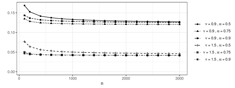
Figure 1. Trend of $\lambda_{i}^{(n)}/(ni^{-2\nu/d-1})$ for $i=n^{\alpha}$ when the points are sampled on the regular grid $[0,1)\cap n^{-1}\mathbb{Z}$. Parameters $\phi$ and $\sigma^{2}$ in Matérn covariogram are set to be $1.0$ and $1.0$, respectively.

Assumption 2.

Let $\chi_{n}=[0,1)^{d}\cap n^{-1/d}\mathbb{Z}^{d}$ be the regular grid. There exists $A=A(\phi,\nu,d)>0$ such that

(10) $$\lambda_{i}^{(n)}/(ni^{-2\nu/d-1})\to A\quad\mbox{ as }\,n,i\to\infty$$

Besides the numerical evidence, let us explain heuristics underlying this assumption from a theoretical viewpoint. First, Assumption 2 has been rigorously proved in Chen et al. (2000) for Ornstein–Uhlenbeck processes, corresponding to the case of $\nu=1/2$ and $d=1$. Furthermore, for the regular grid $\chi_{n}$, the scaled covariance matrix $\frac{1}{n{\sigma^{2}}}K_{n}$ is viewed as the discretization of the integral operator

$$\mathcal{K}f(x):=\int_{[0,1]^{d}}K_{w}(s-t;{1},\phi,\nu)f(t)dt,$$

where $f$ is a test function. The integral operator $\mathcal{K}$ has eigenvalues $\lambda_{1}\geq\lambda_{2}\geq\cdots>0$. Intuitively, $\lambda^{(n)}_{i}/n\approx\lambda_{i}$ which is at least true for fixed $i$. Santin and Schaback (2016) observed that $\lambda_{i}=h_{i-1}^{2}$, with ${h_{i}}$ the $i$-width of the unit Sobolev ball in the $L^{2}$ space. Using a differential operator approach, Jerome (1972) showed that $\lim_{i\rightarrow\infty}i^{\frac{2\nu+d}{2d}}{h_{i}}=C^{\prime}$. The above two results imply that $\lim_{i\rightarrow\infty}i^{2\nu/d+1}\lambda_{i}=C^{\prime 2}$. Thus, we expect that $\lambda^{(n)}_{i}/(ni^{-2\nu/d-1})\approx i^{2\nu/d-1}\lambda_{i}\approx C^{\prime 2}$ as $n,i\rightarrow\infty$, though the error $|\lambda^{(n)}_{i}/n-\lambda_{i}|$ is not easy to estimate.

To proceed further, we need the following lemma which is proved by elementary calculus.

Lemma 2.

Assume that $\max_{s\in S}\min_{1\leq i\leq n}\|s-s_{i}\|\asymp n^{-1/d}$ and $\min_{1\leq i\neq j\leq n}||s_{i}-s_{j}||\asymp n^{-1/d}$. Let $a_{ni}=1/(\widehat{\tau}^{2}_{n}+\widehat{\sigma}_{n}^{2}\lambda_{i}^{(n)})$, $b_{ni}=\lambda_{i}^{(n)}/(\tau^{2}_{0}+\widehat{\sigma}^{2}_{n}\lambda_{i}^{(n)})$, $a^{0}_{ni}=1/(\tau_{0}^{2}+\sigma^{2}\lambda_{i}^{(n)})$, and $b^{0}_{ni}=\lambda_{i}^{(n)}a_{ni}^{0}$.

(1) There exists $C>0$ such that

$$\sum_{i=1}^{n}a^{2}_{ni}\asymp n\;,\;\sum_{i=1}^{n}\lambda_{i}^{(n)}a^{2}_{ni}\leq Cn^{\frac{1}{2\nu/d+1}}\;,\;\sum_{i=1}^{n}b_{ni}\leq Cn^{\frac{1}{2\nu/d+1}}\;,\;\sum_{i=1}^{n}b_{ni}^{2}\leq Cn^{\frac{1}{2\nu/d+1}}\;.$$

(2) Under Assumption 1,

$$\sum_{i=1}^{n}\lambda_{i}^{(n)}a^{2}_{ni}\asymp n^{\frac{1}{2\nu/d+1}}\;,\;\sum_{i=1}^{n}b_{ni}\asymp n^{\frac{1}{2\nu/d+1}}\;,\;\sum_{i=1}^{n}b_{ni}^{2}\asymp n^{\frac{1}{2\nu/d+1}}\;.$$

(3) Under Assumption 2, there exist $c_{1}(\sigma),c_{2}(\sigma),c_{3}(\sigma)>0$ such that as $n\to\infty$,

$$\frac{1}{n}\sum_{i=1}^{n}(a_{ni}^{0})^{2}\to c_{1}(\sigma),\quad\frac{1}{n}\sum_{i=1}^{n}(a_{ni}^{0})^{4}\to c_{2}(\sigma),\quad\frac{1}{n^{1/(1+2\nu/d)}}\sum_{i=1}^{n}(b_{ni}^{0})^{2}\to c_{3}(\sigma).$$

2.2.2. Consistency of the maximum likelihood estimator

We begin our development of the consistency of the maximum likelihood estimator of the nugget $\widehat{\tau}^{2}_{n}$ and the microergodic parameter $\widehat{\sigma}_{n}^{2}\phi_{1}^{2\nu}$ under Assumption 1. We point out that the consistency of the nugget $\widehat{\tau}^{2}_{n}$ is true without Assumption 1 on the lower bound for eigenvalues, and $\widehat{\tau}^{2}_{n}$ remains consistent even when $\sigma^{2}$ and $\phi$ are misspecified.

Theorem 2.4.

Assume that $(\tau_{0}^{2},\sigma_{0}^{2})\in D$, $\chi_{n}:=\{s_{1},\ldots,s_{n}\}$ satisfy

$$\max_{s\in S}\min_{1\leq i\leq n}\|s-s_{i}\|\asymp n^{-1/d}\quad\mbox{and}\quad\min_{1\leq i\neq j\leq n}||s_{i}-s_{j}||\asymp n^{-1/d}.$$

Let $P_{0}$ be the probability measure of the Matérn model with covariogram $K(\cdot;\,\tau_{0}^{2},\sigma_{0}^{2},\phi_{0},\nu)$. Then $\widehat{\tau}_{n}^{2}\rightarrow\tau_{0}^{2}$ almost surely under $P_{0}$. Further assume that the conditions in Assumption 1 hold. Then $\widehat{\sigma}_{n}^{2}\phi_{1}^{2\nu}\rightarrow\kappa_{0}$ almost surely under $P_{0}$.

Proof.

Let $P_{1}$ be the probability measure corresponding to $K(\cdot;\,\tau_{0}^{2},\sigma_{1}^{2},\phi_{1},\nu)$, where $\sigma_{1}^{2}:=\kappa_{0}/\phi_{1}^{2\nu}$. We first prove that $\widehat{\tau}^{2}_{n}\rightarrow\tau^{2}_{0}$ almost surely under $P_{0}$. From Theorem 2.1 we know that $P_{0}\equiv P_{1}$. Hence, it suffices to prove that $\widehat{\tau}^{2}_{n}\rightarrow\tau^{2}_{0}$ almost surely under $P_{1}$. Under $P_{1}$, we can rewrite (5) as

(11) $$\ell(\tau^{2},\widehat{\sigma}_{n}^{2},\phi_{1})=\sum_{i=1}^{n}\frac{\tau^{2}_{0}+\sigma_{1}^{2}\lambda_{i}^{(n)}}{\tau^{2}+\widehat{\sigma}_{n}^{2}\lambda_{i}^{(n)}}W_{i}^{2}+\sum_{i=1}^{n}\log(\tau^{2}+\widehat{\sigma}_{n}^{2}\lambda_{i}^{(n)}),$$

where $W_{i}\stackrel{{\scriptstyle iid}}{{\sim}}\mathcal{N}(0,1)$. The maximum likelihood estimator $\widehat{\tau}_{n}^{2}$ of $\tau^{2}$ satisfies

(12) $$(\tau^{2}_{0}-\widehat{\tau}^{2}_{n})\cdot\sum_{i=1}^{n}W_{i}^{2}a_{ni}^{2}=\sum_{i=1}^{n}\widehat{\tau}^{2}_{n}(1-W_{i}^{2})a_{ni}^{2}+\sum_{i=1}^{n}(\widehat{\sigma}_{n}^{2}-\sigma_{1}^{2}W_{i}^{2})\lambda_{i}^{(n)}a_{ni}^{2}.$$

where $a_{ni}=1/(\widehat{\tau}^{2}_{n}+\widehat{\sigma}_{n}^{2}\lambda_{i}^{(n)})$. By Lemma 2 (1), we have $\sum_{i=1}^{n}a_{ni}^{2}\asymp n$ and $\sum_{i=1}^{n}\lambda_{i}^{(n)}a_{ni}^{2}\leq Cn^{1/(2\nu/d+1)}$ for some $C>0$. Using the results of Etemadi (2006), we obtain

(13) $$\frac{\sum_{i=1}^{n}W_{i}^{2}a_{ni}^{2}}{\sum_{i=1}^{n}a_{ni}^{2}}\rightarrow 1,\quad\frac{\sum_{i=1}^{n}\widehat{\tau}^{2}_{n}(1-W_{i}^{2})a_{ni}^{2}}{\sum_{i=1}^{n}a_{ni}^{2}}\rightarrow 0\quad\mbox{and}\quad\frac{\sum_{i=1}^{n}(\widehat{\sigma}_{n}^{2}-\sigma_{1}^{2}W_{i}^{2})\lambda_{i}^{(n)}a_{ni}^{2}}{\sum_{i=1}^{n}a_{ni}^{2}}\rightarrow 0.$$

Here we also give an elementary proof of the last convergence in (13). It is clear that

$$\mbox{l.h.s}=\frac{\sum_{i=1}^{n}\widehat{\sigma}_{n}^{2}\lambda_{i}^{(n)}a_{ni}^{2}}{\sum_{i=1}^{n}a_{ni}^{2}}-\sigma_{1}^{2}\frac{\sum_{i=1}^{n}\lambda_{i}^{(n)}a_{ni}^{2}W_{i}^{2}}{\sum_{i=1}^{n}a_{ni}^{2}}:=(a)-(b).$$

From (6) we know that $\widehat{\sigma}_{n}^{2}$ is bounded from above. So the term $(a)\lesssim\frac{\sum_{i=1}^{n}\lambda_{i}^{(n)}a_{ni}^{2}}{\sum_{i=1}^{n}a_{ni}^{2}}\to 0$ by Lemma 2 (1). Next

$$Z_{ni}:=\lambda_{i}^{(n)}a_{ni}^{2}=\frac{\lambda_{i}^{(n)}}{(\widehat{\tau}_{n}^{2}+\widehat{\sigma}_{n}^{2}\lambda_{i}^{(n)})^{2}}\leq\frac{\lambda_{i}^{(n)}}{4\widehat{\tau}_{n}^{2}\widehat{\sigma}_{n}^{2}\lambda_{i}^{(n)}}\leq C,$$

again, from (6) we note that $\widehat{\tau}_{n}^{2}$ and $\widehat{\sigma}_{n}^{2}$ are bounded away from $0$. Moreover, by Lemma 2 (1), $\sum_{i=1}^{n}Z_{ni}\lesssim n^{\theta}$ for some $\theta<1$ and so $\sum_{i=1}^{n}Z_{ni}^{2}\lesssim n^{\theta}$ (since $Z_{ni}\leq C$).

Let $S_{n}:=\sum_{i=1}^{n}\frac{Z_{ni}(W_{i}^{2}-1)}{n}$. Fix $\delta>0$. We have

$$\qquad\mathbb{P}\left(\sup_{m+1\leq k\leq n}|S_{k}-S_{m}|\geq\delta\right)\leq\mathbb{P}\left(\sup_{m+1\leq k\leq n}\left|\sum_{i=1}^{m}\left(\frac{Z_{ki}}{k}-\frac{Z_{mi}}{m}\right)(W_{i}^{2}-1)\right|\geq\frac{99}{100}\delta\right)$$

$$\qquad\qquad\qquad\qquad\qquad\qquad\qquad+\mathbb{P}\left(\sup_{m+1\leq k\leq n}\left|\sum_{i=m+1}^{k}\frac{Z_{ki}}{k}(W_{i}^{2}-1)\right|>\frac{\delta}{100}\right):=(c)+(d).$$

For the term $(c)$, we get for some $C^{\prime}>0$,

$$(c) \leq\mathbb{P}\left(\left|\sum_{i=1}^{m}\frac{Z_{mi}}{m}(W_{i}^{2}-1)\right|\geq\frac{99}{200}\delta\right)+\mathbb{P}\left(\sup_{m+1\leq k\leq n}\left|\sum_{i=1}^{m}\frac{Z_{ki}}{k}(W_{i}^{2}-1)\right|\geq\frac{99}{200}\delta\right)$$

$$\leq\mathbb{P}\left(\left|\sum_{i=1}^{m}\frac{Z_{mi}}{m}(W_{i}^{2}-1)\right|\geq\frac{99}{200}\delta\right)+\sum_{k=m+1}^{n}\mathbb{P}\left(\left|\sum_{i=1}^{m}\frac{Z_{ki}}{k}(W_{i}^{2}-1)\right|\geq\frac{99}{200}\delta\right)$$

$$\lesssim\frac{1}{\delta^{2}m^{2-\theta}}+\sum_{k=m+1}^{n}\frac{1}{\delta^{2}k^{2-\theta}}\leq\frac{C^{\prime}}{\delta^{2}m^{1-\theta}}.$$

For the term $(d)$, we have for some $C^{\prime\prime}>0$,

$$(d) \leq\sum_{k=m+1}^{n}\mathbb{P}\left(\left|\sum_{i=m+1}^{k}\frac{Z_{ki}}{k}(W_{i}^{2}-1)\right|>\frac{\delta}{100}\right)\lesssim\sum_{k=m+1}^{n}\frac{1}{\delta^{2}k^{2-\theta}}\leq\frac{C^{\prime\prime}}{\delta^{2}m^{1-\theta}}.$$

Combining the above estimates and passing $n\to\infty$ yield $\mathbb{P}\left(\sup_{n\geq m}|S_{n}-S_{m}|\geq\delta\right)\to 0$ as $m\to\infty$. It follows that $S_{n}$ converges almost surely (see the proof of Theorem 2.5.6 in Durrett (2019)). Since $\sum_{i=1}^{n}Z_{ni}/n\to 0$ by Lemma 2 (1), we have $\sum_{i=1}^{n}Z_{ni}W_{i}^{2}/n$ converges almost surely to some $U\geq 0$ almost surely. By the boundedness of $Z_{ni}$, we get $\sup_{n}\mathbb{E}\left[\left(\sum_{i=1}^{n}Z_{ni}W_{i}^{2}/n\right)^{2}\right]<\infty$ so $\sum_{i=1}^{n}Z_{ni}W_{i}^{2}/n$ is uniformly integrable. Thus, $\mathbb{E}U=\lim_{n\to\infty}\mathbb{E}\left(\sum_{i=1}^{n}Z_{ni}W_{i}^{2}/n\right)=\lim_{n\to\infty}\sum_{i=1}^{n}Z_{ni}/n=0$. So $U=0$ almost surely, and hence $\sum_{i=1}^{n}Z_{ni}W_{i}^{2}/n\to 0$ almost surely. The term $(b)=\frac{\sigma_{1}^{2}\sum_{i=1}^{n}Z_{ni}W_{i}^{2}}{\sum_{i=1}^{n}a_{ni}^{2}}\to 0$ since $\sum_{i=1}^{n}a_{ni}^{2}\asymp n$.

Combining the above with (12), we have $\widehat{\tau}^{2}_{n}\to\tau^{2}_{0}$ almost surely under $P_{1}$.

Next, we show that $\widehat{\sigma}_{n}^{2}\phi_{1}^{2\nu}\rightarrow\kappa_{0}$ almost surely under $P_{0}$. Since $\widehat{\tau}^{2}_{n}\rightarrow\tau^{2}_{0}$ almost surely under $P_{0}$ and $\sigma_{1}^{2}=\kappa_{0}/\phi_{1}^{2\nu}$, it suffices to show that $\widehat{\sigma}^{{}^{\prime}2}_{n}:=\operatorname{argmin}_{\sigma^{2}\in[c,d]}\ell(\tau^{2}_{0},\sigma^{2},\phi_{1})$ converges almost surely to $\sigma_{1}^{2}$ under $P_{0}$. Again, since $P_{0}\equiv P_{1}$, it suffices to show $\widehat{\sigma}^{{}^{\prime}2}_{n}\rightarrow\sigma_{1}^{2}$ almost surely under $P_{1}$. Under $P_{1}$,

(14) $$\ell(\tau^{2}_{0},\sigma^{2},\phi_{1})=\sum_{i=1}^{n}\frac{\tau^{2}_{0}+\sigma_{1}^{2}\lambda_{i}^{(n)}}{\tau^{2}_{0}+\sigma^{2}\lambda^{(n)}_{i}}W_{i}^{2}+\sum_{i=1}^{n}\log(\tau^{2}_{0}+\sigma^{2}\lambda^{(n)}_{i}).$$

Taking the derivative of (14) with respect to $\sigma^{2}$ and equating to zero, we obtain

(15) $$\sum_{i=1}^{n}b_{ni}(W_{i}^{2}-1)=(\widehat{\sigma}^{{}^{\prime}2}_{n}-\sigma_{1}^{2})\sum_{i=1}^{n}b_{ni}^{2}W_{i}^{2}.$$

with $b_{ni}=\lambda_{i}^{(n)}/(\tau^{2}_{0}+\widehat{\sigma}^{{}^{\prime}2}_{n}\lambda_{i}^{(n)})$. It suffices to prove that $\sum_{i=1}^{n}b_{ni}(W_{i}^{2}-1)/\sum_{i=1}^{n}b_{ni}^{2}W_{i}^{2}$ converges almost surely to $0$. Since

$$\frac{\sum_{i=1}^{n}b_{ni}(W_{i}^{2}-1)}{\sum_{i=1}^{n}b_{ni}^{2}W_{i}^{2}}=\frac{\sum_{i=1}^{n}b_{ni}(W_{i}^{2}-1)}{\sum_{i=1}^{n}b_{ni}}\cdot\frac{\sum_{i=1}^{n}b_{ni}}{\sum_{i=1}^{n}b_{ni}^{2}}\cdot\frac{\sum_{i=1}^{n}b_{ni}^{2}}{\sum_{i=1}^{n}b_{ni}^{2}W_{i}^{2}},$$

and $\sum_{i=1}^{n}b_{ni}\asymp n^{1/(2\nu/d+1)}$, $\sum_{i=1}^{n}b_{ni}^{2}\asymp n^{1/(2\nu/d+1)}$ by Lemma 2 (2), we get

$$\frac{\sum_{i=1}^{n}b_{ni}(W_{i}^{2}-1)}{\sum_{i=1}^{n}b_{ni}}\longrightarrow 0\quad\mbox{and}\quad\frac{\sum_{i=1}^{n}b_{ni}^{2}}{\sum_{i=1}^{n}b_{ni}^{2}W_{i}^{2}}\longrightarrow 1\quad a.s.$$

Combining the above estimates with (15), we have $\widehat{\sigma}^{{}^{\prime}2}_{n}\to\sigma_{1}^{2}$ almost surely under $P_{1}$. ∎

It is difficult to establish the consistency of the joint maximum likelihood estimates of $\{\kappa,\tau^{2},\phi\}$ (i.e., $\phi$ is not fixed). A related result can be found in Theorem 2 of Kaufman and Shaby (2013) without a nugget effect. In the presence of a nugget effect, constructing such a proof becomes difficult due to the analytic intractability of the maximum likelihood estimators for $\{\kappa,\tau^{2},\phi\}$. Nevertheless, our simulation studies in Section 3.3 seem to support consistent estimation of $\{\kappa,\tau^{2}\}$ even when $\phi$ is not fixed.

2.2.3. Asymptotic normality of the maxumum likelihood estimator

Given the consistency of the maximum likelihood estimators, we turn to their asymptotic distributions. For simplicity of presentation, we let $S=[0,1]^{d}$ in the following theorem. The asymptotic normality described below holds for any compact set $S\subset\mathbb{R}^{d}$.

Theorem 2.5.

Assume that $n$ is the $d^{th}$ power of some positive integer, $\chi_{n}=[0,1)^{d}\cap n^{-1/d}\mathbb{Z}^{d}$, and the conditions in Assumption 2 hold. Let

$$a^{0}_{ni}:=1/(\tau^{2}_{0}+\sigma_{1}^{2}\lambda_{i}^{(n)})\quad\mbox{and}\quad b^{0}_{ni}:=\lambda_{i}^{(n)}a_{ni}^{0}\quad\mbox{for }\,1\leq i\leq n.$$

There exist constants $c_{1},c_{2},c_{3}>0$ such that as $n\rightarrow\infty$,

(16) $$\frac{1}{n}\sum_{i=1}^{n}(a_{ni}^{0})^{2}\to c_{1},\quad\frac{1}{n}\sum_{i=1}^{n}(a_{ni}^{0})^{4}\to c_{2},\quad\frac{1}{n^{1/(1+2\nu/d)}}\sum_{i=1}^{n}(b_{ni}^{0})^{2}\to c_{3}.$$

We have

(17) $$\sqrt{n}(\widehat{\tau}^{2}_{n}-\tau^{2}_{0})\stackrel{{\scriptstyle(d)}}{{\longrightarrow}}\mathcal{N}(0,2\tau_{0}^{4}c_{2}/c_{1}^{2}),$$

and

(18) $$n^{1/(2+4\nu/d)}(\widehat{\sigma}_{n}^{2}\phi_{1}^{2\nu}-\kappa_{0})\stackrel{{\scriptstyle(d)}}{{\longrightarrow}}\mathcal{N}(0,2\phi_{1}^{4\nu}/c_{3}),$$

under $P_{1}$ corresponding to the Matérn model with covariogram $K(\cdot;\,\tau_{0}^{2},\sigma_{1}^{2},\phi_{1},\nu)$, with $\sigma_{1}^{2}:=\kappa_{0}/\phi_{1}^{2\nu}$.

Proof.

With Assumption 2, the limits in (16) follow from Lemma 2 (3). By (12) and Theorem 2.4, we have

(19) $$\sqrt{n}(\tau^{2}_{0}-\widehat{\tau}^{2}_{n})=(1+o(1))\,\frac{\tau^{2}_{0}\sqrt{n}\sum_{i=1}^{n}(1-W_{i}^{2})(a_{ni}^{0})^{2}+\sigma_{1}^{2}\sqrt{n}\sum_{i=1}^{n}(1-W_{i}^{2})\lambda^{n}_{i}(a^{0}_{ni})^{2}}{\sum_{i=1}^{n}W_{i}^{2}(a_{ni}^{0})^{2}}.$$

We know that $\sum_{i=1}^{n}W_{i}^{2}(a_{ni}^{0})^{2}/\sum_{i=1}^{n}(a_{ni}^{0})^{2}\longrightarrow 1$. In addition,

(20) $$\frac{\tau^{2}_{0}\sqrt{n}\sum_{i=1}^{n}(1-W_{i}^{2})(a_{ni}^{0})^{2}}{\sum_{i=1}^{n}(a_{ni}^{0})^{2}}=\frac{\sum_{i=1}^{n}(1-W_{i}^{2})(a_{ni}^{0})^{2}}{\sqrt{2\sum_{i=1}^{n}(a_{ni}^{0})^{4}}}\cdot\frac{\tau^{2}_{0}\sqrt{2n\sum_{i=1}^{n}(a_{ni}^{0})^{4}}}{\sum_{i=1}^{n}(a_{ni}^{0})^{2}}\stackrel{{\scriptstyle(d)}}{{\longrightarrow}}\mathcal{N}(0,2\tau_{0}^{4}c_{2}/c_{1}^{2}),$$

where the first term on the right hand side converges to $\mathcal{N}(0,1)$ by Lindeberg’s central limit theorem, and the second term converges to $\tau^{2}_{0}\sqrt{2c_{2}}/c_{1}$. Similarly,

(21) $$\frac{\sigma_{1}^{2}\sqrt{n}\sum_{i=1}^{n}(1-W_{i}^{2})\lambda^{n}_{i}(a^{0}_{ni})^{2}}{\sum_{i=1}^{n}(a_{ni}^{0})^{2}}=\frac{\sum_{i=1}^{n}(1-W_{i}^{2})\lambda^{n}_{i}(a^{0}_{ni})^{2}}{\sqrt{2\sum_{i=1}^{n}(\lambda_{i}^{n})^{2}(a^{0}_{ni})^{4}}}\cdot\frac{\sigma_{1}^{2}\sqrt{2n\sum_{i=1}^{n}(\lambda_{i}^{n})^{2}(a^{0}_{ni})^{4}}}{\sum_{i=1}^{n}(a_{ni}^{0})^{2}}\longrightarrow 0,$$

where the first term on the right hand side converges to $\mathcal{N}(0,1)$, and the second term converges to $0$ since $\sum_{i=1}^{n}(\lambda_{i}^{n})^{2}(a^{0}_{ni})^{4}\asymp n^{1/(1+2\nu/d)}$. Combining (19), (20) and (21) leads to (17).

By (15) and Theorem 2.4, we get

(22) $$n^{1/(2+4\nu/d)}(\widehat{\sigma}_{n}^{2}-\sigma_{1}^{2})=(1+o(1))\,\frac{n^{1/(2+4\nu/d)}\sum_{i=1}^{n}b_{ni}^{0}(W_{i}^{2}-1)}{\sum_{i=1}^{n}(b_{ni}^{0})^{2}W_{i}^{2}}.$$

Moreover,

$$\frac{n^{1/(2+4\nu/d)}\sum_{i=1}^{n}b_{ni}^{0}(W_{i}^{2}-1)}{\sum_{i=1}^{n}(b_{ni}^{0})^{2}W_{i}^{2}} =\frac{\sum_{i=1}^{n}b_{ni}^{0}(W_{i}^{2}-1)}{\sqrt{2\sum_{i=1}^{n}(b_{ni}^{0})^{2}}}\cdot\frac{\sqrt{2}n^{1/(2+4\nu/d)}}{\sqrt{\sum_{i=1}^{n}(b_{ni}^{0})^{2}}}\cdot\frac{\sum_{i=1}^{n}(b_{ni}^{0})^{2}}{\sum_{i=1}^{n}(b_{ni}^{0})^{2}W_{i}^{2}}$$

(23) $$\stackrel{{\scriptstyle(d)}}{{\longrightarrow}}\mathcal{N}(0,2/c_{3}),$$

where the first term on the right hand side converges to $\mathcal{N}(0,1)$, the second term converges to $\sqrt{2/c_{3}}$, and the third term converges to $1$. Combining (22) and (2.2.3) yields (18). ∎

Du et al. (2009) showed that for the Matérn model without measurement error, the maximum likelihood estimator $\widehat{\sigma}_{n}^{2}$ converges to $\sigma_{1}^{2}$ at a $\sqrt{n}$-rate. Theorem 2.5 shows that in the presence of measurement error, the maximum likelihood estimator $\widehat{\tau}^{2}_{n}$ has a $\sqrt{n}$-rate while $\widehat{\sigma}_{n}^{2}$ has a slower $n^{1/(2+4\nu/d)}$-rate. This echoes the results of Ying (1991), Chen et al. (2000) with $\nu=\frac{1}{2}$ and $d=1$ for the Ornstein-Uhlenbeck process, where the maximum likelihood estimator $\widehat{\sigma}_{n}^{2}$ converges at a $\sqrt{n}$-rate without measurement error, but at a $\sqrt[4]{n}$-rate in the presence of measurement error.

2.3. Interpolation at new locations

We now turn to predicting the value of the process at unobserved locations. Without the nugget (i.e., $\tau=0$ in (1)), Stein (1988, 1993, 1999) establish that predictions under different measures tend to agree as sample size $n\rightarrow\infty$. However, in the presence of a nugget effect, the predictive variance of $y(s)$ at an unobserved location may not decrease to zero with increasing sample size. In fact, the squared prediction error for any linear predictor is expected to be at least $\tau^{2}$. For example, let $\widehat{y}_{0}=v^{\top}y$ be a linear predictor of $y_{0}=y(s_{0})$ at the unobserved location $s_{0},s_{0}\not\in\chi_{n}$. Let $w=\{w(s_{1}),\ldots,w(s_{n})\}$, $\epsilon=\{\epsilon(s_{1}),\ldots,\epsilon(s_{n})\}$, $w_{0}=w(s_{0})$ and $\epsilon_{0}=\epsilon(s_{0})$. The expected squared prediction error satisfies

$$\mathbb{E}[(\widehat{y}_{0}-y_{0})^{2}] =\mathbb{E}[\{(v^{\top}w-w_{0})+(v^{\top}\epsilon-\epsilon_{0})\}^{2}]=\mathbb{E}[(v^{\top}w-w_{0})^{2}]+\mathbb{E}[(v^{\top}\epsilon-\epsilon_{0})^{2}]\geq\tau^{2}.$$

To see whether there can be a consistent linear (unbiased) estimate of the underlying process $w(\cdot)$ at unobserved locations, consider the universal kriging estimator at an unobserved location $s_{0}$ given by

(24) $$\widehat{Z}_{n}(\tau^{2},\sigma^{2},\phi):=\gamma_{n}(\sigma^{2},\phi)^{\top}\Gamma_{n}(\tau^{2},\sigma^{2},\phi)^{-1}y\;,$$

where $\{\gamma_{n}(\sigma^{2},\phi)\}_{i}:=K_{w}(s_{0}-s_{i};\,\sigma^{2},\phi,\nu)$, and $\{\Gamma_{n}(\tau^{2},\sigma^{2},\phi)\}_{ij}:=K_{w}(s_{i}-s_{j};\,\sigma^{2},\phi,\nu)+\tau^{2}\delta_{0}(i-j)$ for $i,j=1,\ldots,n$. The interpolant $\widehat{Z}_{n}(\tau^{2},\sigma^{2},\phi)$ provides a best linear unbiased estimate of $w_{0}$ under the Matérn model with measurement error (4). By letting $\{K_{n}(\phi)\}_{ij}:=K_{w}(s_{0}-s_{i};\,1,\phi,\nu)$, we have the mean squared error of the estimator (24) follows

(25) $$\operatorname{Var}_{\tau_{0}^{2},\sigma_{0}^{2},\phi_{0}}\{\widehat{Z}_{n}(\tau^{2},\sigma^{2},\phi)-w_{0}\}=\sigma_{0}^{2}\{1-2\gamma_{n}(\sigma^{2},\phi)^{\top}\Gamma_{n}(\tau^{2},\sigma^{2},\phi)^{-1}\gamma_{n}(\sigma_{0}^{2},\phi_{0})\\ +\gamma_{n}(\sigma^{2},\phi)^{\top}\Gamma_{n}(\tau^{2},\sigma^{2},\phi)^{-1}K_{n}(\phi_{0})\Gamma_{n}(\tau^{2},\sigma^{2},\phi)^{-1}\gamma_{n}(\sigma^{2},\phi)\}\\ +\tau_{0}^{2}\gamma_{n}(\sigma^{2},\phi)^{\top}\Gamma_{n}(\tau^{2},\sigma^{2},\phi)^{-2}\gamma_{n}(\sigma^{2},\phi)\;,$$

where $\{\tau_{0}^{2},\sigma_{0}^{2},\phi_{0}\}$ are the true generating values of $\{\sigma^{2},\phi,\tau^{2}\}$. Setting $(\tau^{2},\sigma^{2},\phi)=(\tau_{0}^{2},\sigma_{0}^{2},\phi_{0})$ in (25) yields

(26) $$\operatorname{Var}_{\tau_{0}^{2},\sigma_{0}^{2},\phi_{0}}\{\widehat{Z}_{n}(\tau_{0}^{2},\sigma_{0}^{2},\phi_{0})-w_{0}\}=\sigma_{0}^{2}\{1-\gamma_{n}(\sigma_{0}^{2},\phi_{0})^{\top}\Gamma_{n}(\tau_{0}^{2},\sigma_{0}^{2},\phi_{0})^{-1}\gamma_{n}(\sigma_{0}^{2},\phi_{0})\}$$

Theorem 8 in Chapter 3 of Stein (1999) characterizes the mean squared error of the best linear unbiased estimate at location $0$ as $\displaystyle\frac{(2\pi c)^{1/\alpha}}{\alpha\sin\left({\pi/\alpha}\right)}\left(\delta\tau^{2}\right)^{1-1/\alpha}$ with observations at $\delta j$ for $j\neq 0$. Here $\alpha:=2\nu+1$ and $c:=C\sigma^{2}\phi^{2\nu}$ with $C$ defined in (3). Following the same argument, it is not hard to see that the mean squared error of the best linear unbiased estimate (based on data in $\mathbb{R}^{d}$) is of order $\delta^{2\nu/(2\nu+d)}$. Stein (1999) proved this for observations on the whole line (with a typo in the expression $(44)$ of Stein (1999)). He also conjectured that the above expression for the mean-square error holds for data on any finite interval. We conduct simulations in Section 3.4 with the nugget effect to corroborate this.

2.4. Covariance tapering

Covariance tapering (Furrer et al., 2006; Kaufman et al., 2008; Du et al., 2009) approximates the likelihood by setting certain entries of the covariance matrix to zero to introduce sparsity and, hence, achieve computational benefits. In the presence of a nugget, we explore parameter estimation for the Matérn model (4) with covariance tapering, which, too, have been investigated without the nugget by Wang et al. (2011). Let $K_{\tiny taper}(x;\gamma)$ be a tapering function, which is an isotropic correlation function such that $K_{\tiny taper}(x;\gamma)=0$ for $|x|>\gamma$. The tapered covariogram of the Matérn model with measurement error is given by

(27) $$\widetilde{K}(x;\tau^{2},\sigma^{2},\phi,\nu,\gamma)=K(x;\tau^{2},\sigma^{2},\phi,\nu)\,K_{\tiny taper}(x;\gamma)\;,$$

where $K(x;\tau^{2},\sigma^{2},\phi,\nu)$ is defined in (4). Recalling the notations from Section 2.2, we obtain the tapered covariance matrix of the observations $y=(y_{1},\ldots,y_{n})^{\top}$ as

(28) $$\widetilde{V}_{n}=V_{n}\circ T(\gamma)=\tau^{2}I_{n}+K_{n}\circ T(\gamma),$$

and the (rescaled) negative log-likelihood is $\widetilde{\ell}(\tau,\sigma^{2},\phi):=\log\det\widetilde{V}_{n}+y^{\top}\widetilde{V}_{n}^{-1}y$, where $T(\gamma)$ is the $n\times n$ matrix with $(i,j)$-th entry $K_{\tiny taper}(s_{i}-s_{j};\gamma)$ and $\circ$ denotes the element-wise (Schur or Hadamard) matrix product. For any fixed $\phi_{1}>0$, let $(\widehat{\tau}^{2}_{{\tiny taper},n}(\phi_{1}),\widehat{\sigma}^{2}_{{\tiny taper},n}(\phi_{1}))$ be the maximum likelihood estimators of the tapered Matérn model, i.e.,

(29) $$(\widehat{\tau}^{2}_{{\tiny taper},n}(\phi_{1}),\widehat{\sigma}^{2}_{{\tiny taper},n}(\phi_{1}))=\operatorname{argmin}_{(\tau^{2},\sigma^{2})\in D}\widetilde{\ell}(\tau^{2},\sigma^{2},\phi_{1})\;.$$

To address the identifiability issue of the tapered Matérn model, we require the following assumption on the tapering function which is due to Kaufman et al. (2008).

Assumption 3.

The spectral density $f_{\tiny taper}(u)$ of the tapering function $K_{\tiny taper}(\cdot;\gamma)$ exists, and that there exist $\varepsilon>\max\{\frac{d}{4},1-\nu\}$ and $M_{\varepsilon}<\infty$ such that

(30) $$f_{\tiny taper}(u)\leq\frac{M_{\varepsilon}}{(1+u^{2})^{\nu+\frac{d}{2}+\varepsilon}},\quad u\geq 0.$$

Theorem 2.6.

For $d\leq 3$, let $S\subset\mathbb{R}^{d}$ be a compact set. For $i=1,2$, let $\widetilde{P}_{i}$ be the probability measure of the Gaussian process on $S$ with mean zero and covariance $\widetilde{K}(\cdot;\tau_{i}^{2},\sigma_{i}^{2},\phi_{i},\nu,\gamma)$ defined by (27). Under the conditions in Assumption 3, we have the following results: (i) if $\tau_{1}^{2}\neq\tau_{2}^{2}$, then $\widetilde{P}_{1}\perp\widetilde{P}_{2}$; and (ii) if $\tau_{1}^{2}=\tau_{2}^{2}$, then $\widetilde{P}_{1}\equiv\widetilde{P}_{2}$ if and only if $\sigma_{1}^{2}\phi_{1}^{2\nu}=\sigma_{2}^{2}\phi_{2}^{2\nu}$.

Proof.

We know (Kaufman et al., 2008, Theorem 1) that $\widetilde{P}_{i}\equiv P_{i}$ for $i=1,2$ under Assumption 3. Therefore, the proof is an immediate consequence of our Theorem 2.1 in Section 2. ∎

To progress further, we recall the crucial role of the eigenvalues of $\frac{1}{\sigma^{2}}K_{n}$ in analyzing the maximum likelihood estimators of the Matérn covariogram parameters with measurement error. With covariance tapering, we need estimates on the eigenvalues of $\frac{1}{\sigma^{2}}K_{n}\circ T(\gamma)$. Let $\{\widetilde{\lambda}_{i}^{(n)},i=1,\ldots,n\}$ be the eigenvalues of $\frac{1}{\sigma^{2}}K_{n}\circ T(\gamma)$ in decreasing order. Under Assumption 3, the spectral density $\widetilde{f}$ of the tapered Matérn model with covariogram (27) satisfies $\widetilde{f}(u)\asymp f(u)\asymp u^{-2\nu-d}$ ((B.1) in Kaufman et al. (2008)). By applying Theorem 2.3, we have for $\max_{s\in S}\min_{1\leq i\leq n}\|s-s_{i}\|\asymp n^{-1/d}$,

(31) $$\widetilde{\lambda}_{i}^{(n)}\leq Cni^{-2\nu/d-1}\quad\mbox{for all }i=1,\ldots,n.$$

In order to further study the maximum likelihood estimates of the tapered Matérn model, we need some assumptions on the eigenvalues $\{\widetilde{\lambda}_{i}^{(n)},i=1,\ldots,n\}$. The following two assumptions are analogues of Assumptions 1 and 2.

Assumption 4.

Assume that $\min_{1\leq i\neq j\leq n}||s_{i}-s_{j}||\asymp n^{-1/d}$. There exists $c>0$ such that

(32) $$\widetilde{\lambda}_{i}^{(n)}\geq cni^{-2\nu/d-1}\quad\mbox{ for all }\,i=1,\ldots,n.$$

Assumption 5.

Let $\chi_{n}=[0,1)^{d}\cap n^{-1/d}\mathbb{Z}^{d}$ be the regular grid. There exists $A=A(\phi,\nu,d)>0$ such that

(33) $$\widetilde{\lambda}_{i}^{(n)}/(ni^{-2\nu/d-1})\to A\quad\mbox{ as }\,n,i\to\infty$$

In Figure 2 we plot the values of $\widetilde{\lambda}_{i}^{(n)}/(ni^{-2\nu-1})$ with sampled points on the regular grid $[0,1)\cap n^{-1}\mathbb{Z}$ for $\nu=0.9,1.5$, $n$ ranging from $500$ to $4000$, and $i=n^{0.7}$, $n^{0.8}$, $n^{0.9}$. The tapering function for obtaining $\widetilde{\lambda}_{i}^{(n)}$ is a stationary Wendland function $K_{taper}(x;\gamma)=(1-|x|/\gamma)_{+}^{4}(1+4|x|/\gamma)$ where $\gamma=0.5$ (Wendland, 1995). Consistent with Assumption 4 & 5, the profile plots of $\widetilde{\lambda}_{i}^{(n)}/(ni^{-2\nu/d-1})$ flatten as $n$ increases and the quantity $\widetilde{\lambda}_{i}^{(n)}/(ni^{-2\nu-1})$ tends to converge as $n,i$ become large.

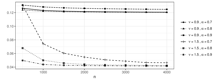
Figure 2. Trend of $\widetilde{\lambda}_{i}^{(n)}/(ni^{-2\nu/d-1})$ for $i=n^{\alpha}$ when the points are sampled on the regular grid $[0,1)\cap n^{-1}\mathbb{Z}$. Parameters $\phi$ and $\sigma^{2}$ in Matérn covariogram are set to be $1.0$ and $1.0$, respectively.

Now we state the consistency results for the maximum likelihood estimators of the tapered Matérn model.

Theorem 2.7.

Assume that $(\tau_{0}^{2},\sigma_{0}^{2})\in D$, $\chi_{n}:=\{s_{1},\ldots,s_{n}\}$ satisfy

$$\max_{s\in S}\min_{1\leq i\leq n}\|s-s_{i}\|\asymp n^{-1/d}\quad\mbox{and}\quad\min_{1\leq i\neq j\leq n}||s_{i}-s_{j}||\asymp n^{-1/d},$$

and the conditions in Assumption 3 hold. Let $\widetilde{P}_{0}$ be the probability measure of the tapered Matérn model with covariogram $\widetilde{K}(\cdot;\tau_{0}^{2},\sigma_{0}^{2},\phi_{0},\nu,\gamma)$.

1. We have $\widehat{\tau}_{{\tiny taper},n}^{2}\rightarrow\tau_{0}^{2}$ almost surely under $\widetilde{P}_{0}$.

2. Assume that the conditions in Assumption 4 hold. Then $\widehat{\sigma}_{{\tiny taper},n}^{2}\phi_{1}^{2\nu}\rightarrow\kappa_{0}$ almost surely under $\widetilde{P}_{0}$

3. Assume that $n$ is the $d^{th}$ power of some positive integer, $\chi_{n}=[0,1)^{d}\cap n^{-1/d}\mathbb{Z}^{d}$, and the conditions in Assumptions 3 and 5 hold. Let $\widetilde{a}^{0}_{ni}:=1/(\tau^{2}_{0}+\sigma_{1}^{2}\widetilde{\lambda}_{i}^{(n)})$ and $\widetilde{b}^{0}_{ni}:=\widetilde{\lambda}_{i}^{(n)}a_{ni}^{0}$ for $\,1\leq i\leq n$. Then, there exist constants $\widetilde{c}_{1},\widetilde{c}_{2},\widetilde{c}_{3}>0$ such that as $n\rightarrow\infty$,

   (34) $$\frac{1}{n}\sum_{i=1}^{n}(\widetilde{a}^{0}_{ni})^{2}\to\widetilde{c}_{1},\quad\frac{1}{n}\sum_{i=1}^{n}(\widetilde{a}^{0}_{ni})^{4}\to\widetilde{c}_{2},\quad\frac{1}{n^{1/(1+2\nu/d)}}\sum_{i=1}^{n}(\widetilde{b}^{0}_{ni})^{2}\to\widetilde{c}_{3}.$$

   We also have

   (35) $$\sqrt{n}(\widehat{\tau}^{2}_{{\tiny taper},n}-\tau^{2}_{0})\stackrel{{\scriptstyle(d)}}{{\longrightarrow}}\mathcal{N}(0,2\tau_{0}^{4}\widetilde{c}_{2}/\widetilde{c}_{1}^{2}),$$

   and

   (36) $$n^{1/(2+4\nu/d)}(\widehat{\sigma}_{{\tiny taper},n}^{2}\phi_{1}^{2\nu}-\kappa_{0})\stackrel{{\scriptstyle(d)}}{{\longrightarrow}}\mathcal{N}(0,2\phi_{1}^{4\nu}/\widetilde{c}_{3}).$$

   under $\widetilde{P}_{1}$ corresponding to the tapered Matérn model with covariogram $\widetilde{K}(\cdot;\,\tau_{0}^{2},\sigma_{1}^{2},\phi_{1},\nu,\gamma)$, with $\sigma_{1}^{2}:=\kappa_{0}/\phi_{1}^{2\nu}$.

Proof.

From Theorem 2.6, we know that $\widetilde{P}_{0}\equiv\widetilde{P}_{1}$. Under $\widetilde{P}_{1}$, the (rescaled) negative log-likelihood is written as

(37) $$\ell(\tau^{2},\widehat{\tau}^{2}_{{\tiny taper},n},\phi_{1})=\sum_{i=1}^{n}\frac{\tau^{2}_{0}+\sigma_{1}^{2}\widetilde{\lambda}_{i}^{(n)}}{\tau^{2}+\widehat{\sigma}^{2}_{{\tiny taper},n}\widetilde{\lambda}_{i}^{(n)}}W_{i}^{2}+\sum_{i=1}^{n}\log(\tau^{2}+\widehat{\sigma}^{2}_{{\tiny taper},n}\widetilde{\lambda}_{i}^{(n)})\;,$$

where $W_{i}\stackrel{{\scriptstyle iid}}{{\sim}}\mathcal{N}(0,1)$. The remainder of the proof follows analogously to Theorems 2.4 and 2.5 by using Assumptions 4 and 5 instead of Assumptions 1 and 2. ∎

2.5. Consistency and asymptotic normality for $d\geq 5$

In contrast to $d\leq 3$, the parameters $\{\tau^{2},\sigma^{2},\phi\}$ are consistently estimable for $d\geq 5$. It is, therefore, of interest to establish if the maximum likelihood estimators of $\{\tau^{2},\sigma^{2},\phi\}$ are consistent in $d\geq 5$. Here we consider a slightly weaker version of the problem which should offer sufficient insights into methods for Gaussian processes for $d\geq 5$.

Recall the development in Section 2.2. Since the scale parameter $\phi_{0}$ is consistently estimable, there exists an estimator $\widehat{\phi}^{\prime}_{n}$ such that $\widehat{\phi}^{\prime}_{n}\to\phi_{0}$ almost surely ($\widehat{\phi}^{\prime}_{n}$ can be any consistent estimator of $\phi_{0}$). Let $(\widehat{\tau}^{2}(\widehat{\phi}^{\prime}_{n}),\widehat{\sigma}^{2}_{n}(\widehat{\phi}^{\prime}_{n}))$ be the maximum likelihood estimators based on the estimator $\widehat{\phi}^{\prime}_{n}$:

(38) $$(\widehat{\tau}^{2}(\widehat{\phi}^{\prime}_{n}),\widehat{\sigma}^{2}_{n}(\widehat{\phi}^{\prime}_{n}))=\operatorname{argmin}_{(\tau^{2},\sigma^{2})\in D}\ell(\tau^{2},\sigma^{2},\widehat{\phi}^{\prime}_{n}).$$

The next theorem establishes consistency of the maximum likelihood estimators $(\widehat{\tau}^{2}(\widehat{\phi}^{\prime}_{n}),\widehat{\sigma}^{2}_{n}(\widehat{\phi}^{\prime}_{n}))$.

Theorem 2.8.

Assume that $(\tau_{0}^{2},\sigma_{0}^{2})\in D$ and the locations in $\chi_{n}:=\{s_{1},\ldots,s_{n}\}$ satisfy

$$\max_{s\in S}\min_{1\leq i\leq n}\|s-s_{i}\|\asymp n^{-1/d}\quad\mbox{and}\quad\min_{1\leq i\neq j\leq n}||s_{i}-s_{j}||\asymp n^{-1/d}.$$

Let $P_{0}$ be the probability measure of the tapered Matérn model with covariogram $K(\cdot;\tau_{0}^{2},\sigma_{0}^{2},\phi_{0},\nu)$.

1. We have $\widehat{\tau}^{2}(\widehat{\phi}^{\prime}_{n})\rightarrow\tau_{0}^{2}$ almost surely under $P_{0}$.

2. Under Assumption 1, $\widehat{\sigma}^{2}_{n}(\widehat{\phi}^{\prime}_{n})\rightarrow\sigma_{0}^{2}$ almost surely under $P_{0}$.

3. Let $n$ be the $d^{th}$ power of some positive integer, $\chi_{n}=[0,1)^{d}\cap n^{-1/d}\mathbb{Z}^{d}$, and suppose Assumption 2 holds. Let $\overline{a}^{0}_{ni}:=1/(\tau^{2}_{0}+\sigma_{0}^{2}\lambda_{i}^{(n)})$ and $\overline{b}^{0}_{ni}:=\lambda_{i}^{(n)}\overline{a}_{ni}^{0}$ for $1\leq i\leq n$. Then, there exist constants $\overline{c}_{1},\overline{c}_{2},\overline{c}_{3}>0$ such that as $n\rightarrow\infty$,

   (39) $$\frac{1}{n}\sum_{i=1}^{n}(\overline{a}_{ni}^{0})^{2}\to\overline{c}_{1},\quad\frac{1}{n}\sum_{i=1}^{n}(\overline{a}_{ni}^{0})^{4}\to\overline{c}_{2},\quad\frac{1}{n^{1/(1+2\nu/d)}}\sum_{i=1}^{n}(\overline{b}_{ni}^{0})^{2}\to\overline{c}_{3}.$$

   We also have

   (40) $$\sqrt{n}(\widehat{\tau}^{2}(\widehat{\phi}^{\prime}_{n})-\tau^{2}_{0})\stackrel{{\scriptstyle(d)}}{{\longrightarrow}}\mathcal{N}(0,2\tau_{0}^{4}\overline{c}_{2}/\overline{c}_{1}^{2}),$$

   and

   (41) $$n^{1/(2+4\nu/d)}(\widehat{\sigma}^{2}_{n}(\widehat{\phi}^{\prime}_{n})-\sigma_{0}^{2})\stackrel{{\scriptstyle(d)}}{{\longrightarrow}}\mathcal{N}(0,2/\overline{c}_{3}).$$

Proof.

To study the asymptotic properties of $(\widehat{\tau}^{2}(\widehat{\phi}^{\prime}_{n}),\widehat{\sigma}^{2}_{n}(\widehat{\phi}^{\prime}_{n}))$, it suffices to consider $(\widehat{\tau}^{2}(\phi_{0}),\widehat{\sigma}^{2}_{n}(\phi_{0}))=\operatorname{argmin}_{(\tau^{2},\sigma^{2})\in D}\ell(\tau^{2},\sigma^{2},\phi_{0})$. Recalling that $P_{0}$ is the probability measure of the Matérn model with covariogram $K(\cdot;\tau_{0}^{2},\sigma_{0}^{2},\phi_{0},\nu)$, the (rescaled) negative log-likelihood (5) is written as

(42) $$\ell(\tau^{2},\sigma^{2},\phi_{0})=\sum_{i=1}^{n}\frac{\tau^{2}_{0}+\sigma_{0}^{2}\lambda_{i}^{(n)}}{\tau^{2}+\sigma^{2}\lambda_{i}^{(n)}}W_{i}^{2}+\sum_{i=1}^{n}\log(\tau^{2}+\sigma^{2}\lambda_{i}^{(n)})$$

under $P_{0}$, where $W_{i}\stackrel{{\scriptstyle iid}}{{\sim}}\mathcal{N}(0,1)$. The reasoning in Theorems 2.4 and 2.5 shows that $(\widehat{\tau}^{2}(\phi_{0}),\widehat{\sigma}^{2}_{n}(\phi_{0}))$ are consistent and are asymptotically normal under various assumptions. As a result, the same holds for $(\widehat{\tau}^{2}(\widehat{\phi}^{\prime}_{n}),\widehat{\sigma}^{2}_{n}(\widehat{\phi}^{\prime}_{n}))$. This completes the proof. ∎

3. Simulations

3.1. Set-up

The preceding results help explain the behaviour of the inference from (1) as the sample size increases within a fixed domain. Here, we present some simulation experiments to illustrate statistical inference for finite samples. We simulate data sets based on (1) in a unit square setting $\nu=1/2$ and $\sigma^{2}=1$. We pick three different values of the nugget, $\tau^{2}\in\{0,0.2,0.8\}$, and choose the decay parameter $\phi$ so that the effective spatial range is $0.15$, $0.4$ or $1$, i.e., the correlation decays to $0.05$ at a distance of $0.15$, $0.4$ or $1$ units. Therefore, we consider $3\times 3=9$ different parameter settings. For each parameter setting, we simulate $1000$ realizations of the Gaussian process over $n=1600$ observed locations. The observed locations are chosen from a perturbed grid. We construct a $67\times 67$ regular grid with coordinates from 0.005 to 0.995 in increments of 0.015 in each dimension. We add a uniform $[-0.005,0.005]^{2}$ perturbation to each grid point to ensure at least 0.005 units separation from its nearest neighbour. We then choose $n=1600$ locations out of the perturbed grid. Codes for studies in this Section are available on https://github.com/LuZhangstat/nugget_consistency.

3.2. Likelihood comparisons

Theorem 2.1 suggests that it is difficult to distinguish between the two Matérn models with measurement error when their microergodic parameters $\{\kappa,\tau^{2}\}$ are close to each other. This property should be reflected in the behaviour of the likelihood function for a large finite sample. To see this, we plot interpolated maps of the log-likelihood among different grids of parameter values. We consider the three values of $\tau_{0}^{2}$ in Section 3.1 and $\phi_{0}=7.49$, which implies an effective spatial range of approximately $0.4$ units, and pick $n=900$ observations from the first realization generated from (1). This yields three different data sets corresponding to the three values of $\tau_{0}^{2}$. We map the negative one-half of the log-likelihood in (5).

The interpolated maps of the log-likelihood are provided in Fig. 3 as a function of $(\tau^{2},\phi)$ in the first two rows and of $(\sigma^{2},\phi)$ in the third row. The first column presents cases with $\tau_{0}=0$, while the second and the third columns are for $\tau_{0}=0.2$ and $0.8$, respectively. The grid for $\phi$ ranges from $2.5$ to $30$ so that the effective spatial ranges between $0.1$ and $1.2$. We specify the range of $\tau^{2}$ and $\sigma^{2}$ to be $(0.0,1.0)$ and $(0.2,4.2)$, respectively, so that the pattern of the log-likelihood map around the true generating values of parameters can be captured. All the interpolated maps, including the contour lines, are drawn to the same scale.

The first row of Figure 3 corresponds to $\sigma^{2}=\sigma^{2}_{0}=1$, the second row corresponds to $\kappa=\kappa_{0}$ and the third row corresponds to $\tau^{2}=\tau_{0}^{2}$. In the first row, we observe that similar log-likelihoods are located along parallel lines $\phi+\tau^{2}=Const$. This suggests that one can identify the maximum with either a fixed $\phi$ or $\tau^{2}$ when $\sigma^{2}=\sigma^{2}_{0}$. In the second row, we find that contours for high log-likelihood values are situated around the actual generating value of the nugget, supporting the identifiability of the nugget as provided in Theorem 2.1. The log-likelihood along the $\phi$-axis has a flat tail as $\phi$ decreases when fixing the nugget, which indicates having the same value of the microergodic parameter $\kappa=\sigma^{2}\phi^{2\nu}$ can result in equivalent probability measures (Theorem 2.1). Finally, the third row reveals that the log-likelihood closely follows the curve $\sigma^{2}\phi=Const$, thereby corroborating Theorem 2.1.

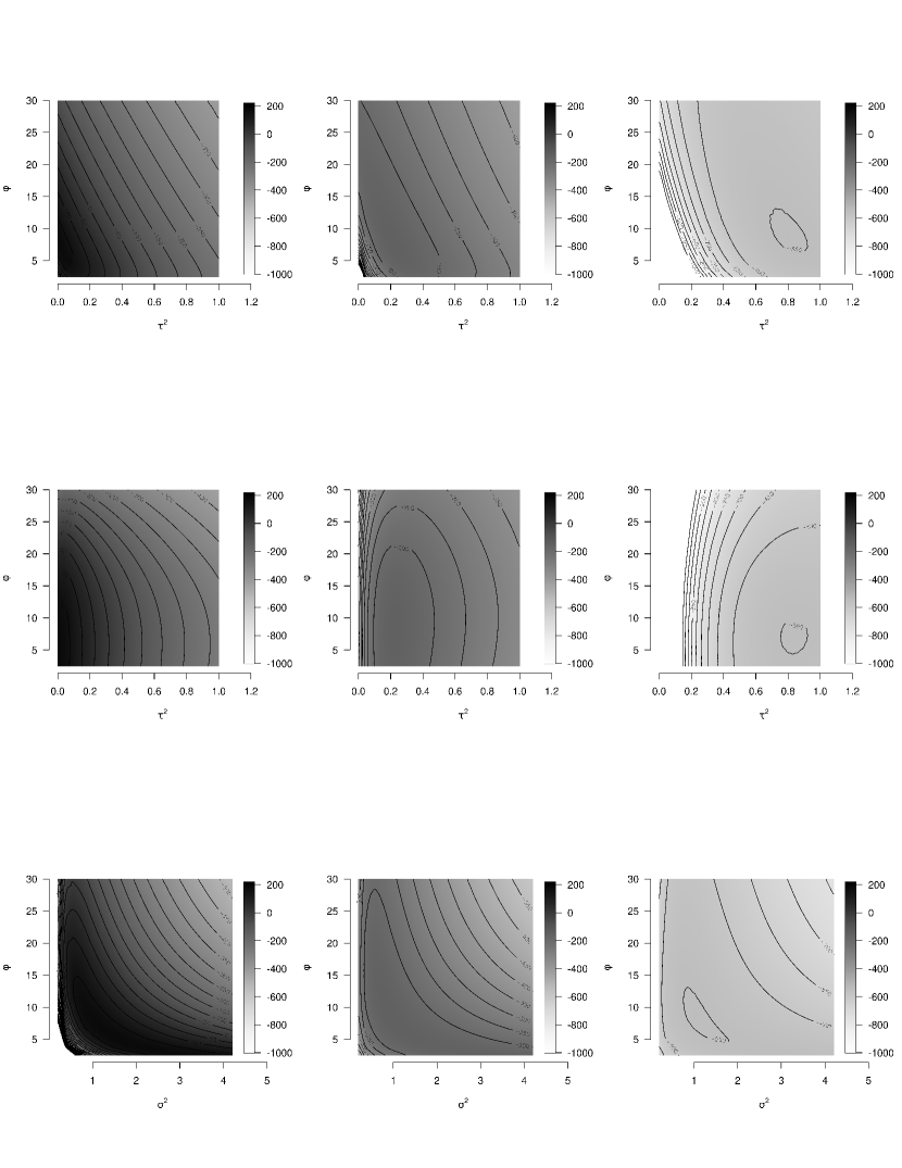
Figure 3. Interpolated maps of the log-likelihood. Darker shades indicate higher values. The first row corresponds to $\sigma^{2}=\sigma^{2}_{0}=1$, the second row corresponds to $\sigma^{2}\phi=\phi_{0}=7.49$, and the third row corresponds to $\tau_{0}=\tau^{2}_{0}$. The columns correspond to $\tau_{0}=0.0$, $\tau_{0}=0.2$, and $\tau_{0}=0.8$, respectively.

3.3. Parameter estimation

We use maximum likelihood estimators to illustrate the asymptotic properties of the parameter estimates. To find the maximum likelihood estimators of $\{\sigma^{2},\tau^{2},\phi,\kappa\}$, we use the log of the profile likelihood for $\phi$ and $\eta=\tau^{2}/\sigma^{2}$, given by

(43) $$\log\{\mathcal{PL}(\phi,\eta)\}\propto - \frac{1}{2}\log[\det\{\rho(\phi)+\eta I_{n}\}]-\frac{n}{2}$$

$$- \frac{n}{2}\log\left[\frac{1}{n}y^{\top}\{\rho(\phi)+\eta I_{n}\}^{-1}y\right]$$

where $\log\{\mathcal{PL}(\phi,\eta)\}=\log[\underset{\sigma^{2}}{\sup}\{\mathcal{L}(\sigma^{2},\phi,\eta)\}]$, $\rho(\phi)$ is the correlation matrix of the underlying process $w(\cdot)$ over observed locations $\chi_{n}$. We optimize (43) to obtain maximum likelihood estimators $\widehat{\phi}$ and $\widehat{\eta}$. The maximum likelihood estimator for $\sigma^{2}$ is $\widehat{\sigma}_{n}^{2}=y^{\top}\{\rho(\widehat{\phi})+\widehat{\eta}I_{n}\}^{-1}y/n$. Calculations were executed using the R function optimx using the Broyden-Fletcher-Goldfarb-Shanno algorithm (Fletcher, 2013) with $\phi>0$ and $\eta>0$, and $\eta=0$ for models without a nugget.

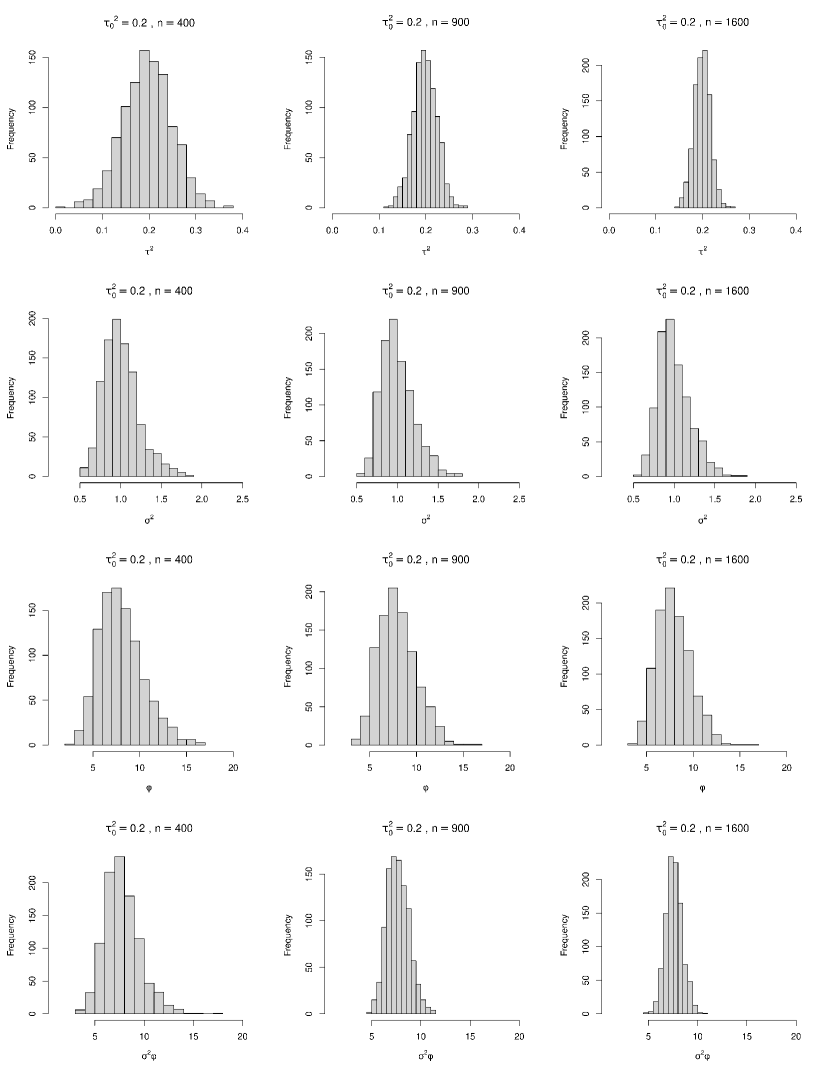
Figure 4. Histograms of $\tau^{2}$ (top row), $\sigma^{2}$ (second row), $\phi$ (third row) and $\kappa=\sigma^{2}\phi^{2\nu}$ (fourth row) obtained from simulation experiments with $\phi_{0}=7.49,\tau_{0}^{2}=0.2$.

We calculate estimators for $\{\tau^{2},\phi,\sigma^{2},\kappa\}$ for each realization with sample sizes 400, 900 and 1600. For each parameter setting and sample size, there are 1000 estimators for $\{\tau^{2},\phi,\sigma^{2}\}$ and $\kappa$. Figure 4 depicts the histograms for the maximum likelihood estimators for $\tau^{2}$, $\phi$, $\sigma^{2}$ and $\kappa$ obtained from simulations with the parameter setting $\{\phi_{0},\tau^{2}_{0}\}=\{7.49,0.2\}$. There is an obvious shrinkage of the variance of estimators for $\tau^{2}$ and $\kappa$ as we increase the sample size from 400 to 1600. We also observe that their distribution becomes more symmetric with an increasing sample size. In contrast, the variance of the estimators for $\sigma^{2}$ and $\phi$ do not have a significant decrease as sample size increases. This is supported by the infill asymptotic results. The maximum likelihood estimators for $\tau^{2}$ and $\kappa$ are consistent and asymptotically normal. The maximum likelihood estimators for $\phi$ and $\sigma^{2}$ are not consistent and, hence, their variances do not decrease to zero with increasing sample size.

Table 1–4 list percentiles, biases, and sample standard deviations for the estimates of $\tau^{2}$, $\phi$, $\sigma^{2}$ and $\kappa$ for each of the 9 parameter settings and offer further insights about the finite sample inference. When the spatial correlation is strong ($\phi$ is small), $\widehat{\tau}^{2}$ tends to be more precise, while $\widehat{\sigma}^{2}$ tends to have more variability. Unsurprisingly, the measurement error is easily distinguished from a less variable latent process $w(\cdot)$. Highly correlated realizations of $w(\cdot)$ results in less precise inference for $\sigma^{2}$. If the nugget is larger, then the estimators for $\phi$, $\sigma^{2}$ and $\kappa$ are less precise; the presence of measurement error weakens the precision of the estimates.

3.4. Interpolation

We use the kriging estimator in (24) and its mean squared prediction error (MSPE) in (25) to explore spatial interpolation in the presence of the nugget. We use (24) to predict the underlying process $w(\cdot)$ over unobserved locations. From Theorem 8 in Chapter 3 of Stein (1999), we expect a clear trend of convergence for $d=1$. Let $\nu=1/2$, $\tau_{0}^{2}=0.2$, $\sigma_{0}^{2}=1.0$ and $\phi_{0}=7.49$. We use (1) to generate observations over $12,000$ randomly picked locations in $[0,1]$. We compute the MSPE using 3 hold-out points $\{0.25,0.5,0.75\}\in[0,1]$ for different subsets of the data with sample sizes ranging from $500$ to $12,000$. Figure 5(a) shows that the MSPE tends to approach $0$ as sample size increases. This corroborates Stein’s conjecture that the underlying process $w(\cdot)$ in (1) can be consistently estimated on a finite interval.

Next, we use the simulated data set with $n=1600$ locations over the unit square used in Section 3.3. We calculate the MSPE using (25) and (26) over a $50\times 50$ regular grid of locations over $[0,1]^{2}$. This is repeated for different data sets with sample sizes varying between 400 and 1600. Figure 5(b) shows that the MSPE decreases as sample size increases. This trend still holds when the predictor is formed under misspecified models, a finding similar to those in Kaufman and Shaby (2013) without the nugget. If $\nu$ is fixed at the true generating value, then predictions under any parameter setting are consistent and asymptotically efficient with no nugget effect. The proof in Kaufman and Shaby (2013) is based on Stein (1993), hence their results do not carry over to our setting due to the discontinuity in our covariogram at $0$. (This technical difficulty was also pointed out by (Yakowitz and Szidarovszky, 1985, p.38)). However, their results suggest empirical studies to explore the asymptotic properties of interpolation.

To compare with results in Kaufman and Shaby (2013, Section 2.3), we examine two ratios

$$\mbox{i)}\quad\frac{\operatorname{Var}_{\tau_{0}^{2},\sigma_{0}^{2},\phi_{0}}\{\widehat{z}_{n}(\tau_{1}^{2},\sigma_{1}^{2},\phi_{1})-w_{0}\}}{\operatorname{Var}_{\tau_{0}^{2},\sigma_{0}^{2},\phi_{0}}\{\widehat{z}_{n}(\tau_{0}^{2},\sigma_{0}^{2},\phi_{0})-w_{0}\}},\quad\mbox{and ii)}\quad\frac{\operatorname{Var}_{\tau_{1}^{2},\sigma_{1}^{2},\phi_{1}}\{\widehat{z}_{n}(\tau_{0}^{2},\sigma_{1}^{2},\phi_{1})-w_{0}\}}{\operatorname{Var}_{\tau_{0}^{2},\sigma_{0}^{2},\phi_{0}}\{\widehat{z}_{n}(\tau_{0}^{2},\sigma_{1}^{2},\phi_{1})-w_{0}\}}.$$

Figure 5(c) compares the ratio defined by i). This ratio tends to approach 1 only when $\tau_{1}^{2}=\tau_{0}^{2}$ and $\kappa=\kappa_{0}$. Unlike the case with no nugget, asymptotic efficiency is only observed when the estimator is fitted under models with Gaussian measures equivalent to the generating Gaussian measure. Figure 5(d) plots the ratio defined by ii). As in Fig. 5(c), this ratio also tends to approach 1 only when $\tau_{1}^{2}=\tau_{0}^{2}$, $\kappa=\kappa_{0}$. Based on our simulation study, we posit that the asymptotic efficiency and asymptotically correct estimation of MSPE hold only when $\tau_{1}^{2}=\tau_{0}^{2}$, $\kappa=\kappa_{0}$.

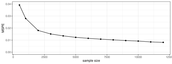
(a)

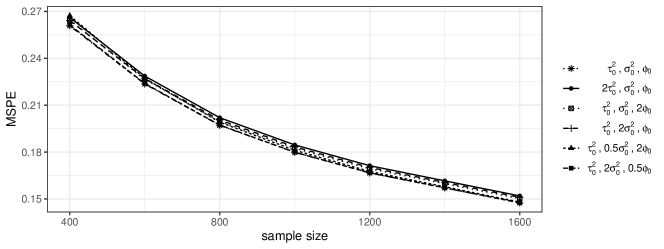
(b)

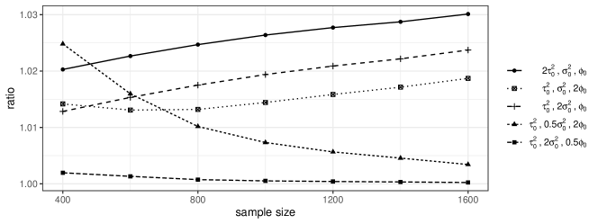
(c)

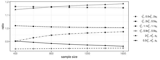
(d)

Figure 5. The MSPE for $w(\cdot)$ at (a) unobserved locations with study domain $[0,1]$ (b) a $50\times 50$ grid over $[0,1]^{2}$. The ratio of mean square predict error (ratio) for testing asymptotic efficiency (c) and asymptotically correct estimation of MSPE (d)

3.5. Bayesian inference from finite samples

The asymptotic results in the preceding sections imply that a misspecified value of $\phi$ does not violate the consistency and asymptotic normality of the maximum likelihood estimator of the nugget $\tau^{2}$ or of the microergodic parameter $\kappa=\sigma^{2}\phi^{2\nu}$. In order to assess the extent to which these asymptotic results can guide practical implementation of model fitting for finite samples, we conduct a sensitivity test to check the stability of the inferences of $\tau^{2}$ and $\kappa$ from finite samples under different specifications for $\phi$. Here, we present inferences for $\tau^{2}$ and $\kappa$ based on a Bayesian analysis using finite samples.

We generate data over $n=1,600$ observed locations situated on the perturbed grid described in Section 3.1. We use a zero-centered Matérn model with measurement error to generate the data, where $\nu=1/2$, $\sigma^{2}=1$, $\tau^{2}=0.5$ and $\phi=9.98$. We fit the simulated data through a zero-centered Matérn model with measurement error with $\textrm{IG}(2,1/2)$ and $\textrm{IG}(2,1)$ priors for $\tau^{2}$ and $\sigma^{2}$, respectively. When assuming $\phi$ is unknown, we use a Gamma prior with shape 2 and rate $2/\phi_{0}$ for $\phi$, where $\phi_{0}$ is the true value of $\phi$ for the simulated data. We specified prior distributions with means equal to the data generating parameter values. We also fit the model with $\phi$ equal to 0.2, 0.5, 1, 2, and 5 times the value of $\phi_{0}$. We randomly select $n=400$, $900$ and $1,600$ samples for model fitting. The posterior inferences are based on 4 MCMC chains, each with 500 iterations for burn-in and 500 iterations for sampling. All models are implemented in cmdstanr (Gabry and Češnovar, 2020). The reported $\hat{R}$ (R-hat) values for all parameters are no more than 1.02 and the reported effective sample size for all parameters are greater than 400, showing adequate convergence of all MCMC chains.

Figure 6 illustrates the posterior distributions of $\tau^{2}$ and $\kappa$. As expected from Theorem 7, the variance of the posterior distributions decrease with increasing values of $n$. The posterior distributions for $\kappa$ and $\tau^{2}$ approach the truth as $n$ increases, but the inference can be highly biased when $\phi$ is misspecified. The results for $\kappa$ are similar to those reported by Kaufman and Shaby (2013) for a zero-centered Matérn model without measurement error. We observe stabler posterior inference of $\tau^{2}$ than $\kappa$ for the cases when $\phi$ is unknown or fixed at values no more than $\phi_{0}$. The case when $\phi=5\phi_{0}$ calls for some additional remarks. Here, the effective spatial range (i.e., the distance beyond which the spatial correlation drops to $0.05$) is only about $4\%$ of the maximum inter-site distance in our domain. Hence, the spatial correlation is negligible making it difficult to distinguish the nugget $\tau^{2}$ from the “partial sill” $\sigma^{2}$ and inference is sensitive to the prior specification. This is a plausible explanation for the poorer estimates of $\tau^{2}$ when $\phi=5\phi_{0}$.

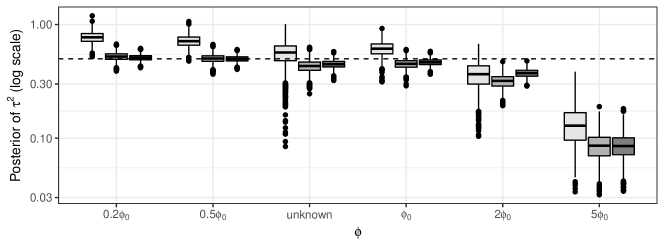
(a)

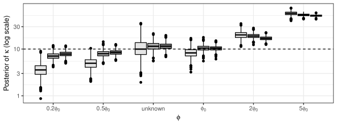
(b)

Figure 6. Posterior distributions for (a) $\tau^{2}$ and (b) $\kappa$ obtained from the simulation studies in Section 3.5. The decay parameter is either estimated via MCMC sampling (unknown), fixed at the true value $\phi_{0}$, or fixed at a multiples of $\phi_{0}$, viz. $\{0.2\phi_{0},\ldots,5\phi_{0}\}$. The three boxplots in each group correspond to sample sizes of $n=400$, $900$, and $1,600$ reading from left to right. The dashed line indicates the true value.

4. Discussion

We have developed insights into inference under infill asymptotics of Gaussian process parameters in the context of spatial or geostatistical analysis in the presence of the nugget effect. Our work can be regarded as an extension of similar investigations without the nugget effect. While geostatistical modelling usually applies to $\mathbb{R}^{d}$ with $d\leq 3$, we have also developed some new insights into $d\geq 5$, where consistency of the MLE’s for the Matérn model remains unresolved even without the nugget.

We have discussed the complications in establishing consistency and asymptotic efficiency in parameter estimation and spatial prediction due to the discontinuity introduced by the nugget. Tools in standard spectral analysis no longer work in this scenario. Understanding the behaviour of such processes will enhance our understanding of identifiability of process parameters. For example, the failure to consistently estimate certain (non-microergodic) parameters can also be useful for Bayesian inference where we can conclude that the effect of the likelihood will never overwhelm the prior when calculating the posterior distribution of non-microergodic parameters. Section 3.5 presented some insights into the behaviour of Bayesian estimates for the nugget in the presence of a misspecified range parameter. Formal investigations into the consistency of the posterior distributions of Matérn covariogram parameters are certainly of interest and can be built upon some of our developments in the current manuscript.

We anticipate further research in variants of geostatistical models with the nugget. For example, one can explore whether some results, such as Theorem 2 in Kaufman and Shaby (2013) where $\phi$ is estimated, will hold for the Matérn model with the nugget. Our simulations also suggest further research in asymptotic efficiency provided in Theorem 3 of Kaufman and Shaby (2013) in the presence of the nugget. With recent interest in scalable Gaussian process models, we can investigate asymptotic properties of approximations indicated on the lines of Vecchia (1988) and Section 10.5.3 in Zhang (2012); (also see Banerjee, 2017, for scalable spatial process models in Bayesian settings). In Bayesian contexts, understanding posterior consistency for the nugget will offer insights into classes of priors. Finally, we point out that the conditions in Assumptions 1 and 2 about eigenvalue estimates are expected and their rigorous proofs will constitute future research, as will further theoretical explorations on Gaussian processes in $\mathbb{R}^{d}$ for all values of $d$.. In particular, a rigorous proof of Assumption 2 is challenging and will be of interest in general kernel methods and bandit problems.

Table 1. Summary of estimates of $\tau^{2}$: percentiles, bias, and sample standard deviations (SD).

$\tau^{2}_{0}$	$\phi_{0}$	n	5%	25%	50%	75%	95%	BIAS	SD
0.200	19.972	400	0.000	0.111	0.189	0.269	0.382	-0.007	0.112
		900	0.102	0.159	0.197	0.235	0.289	-0.004	0.056
		1600	0.141	0.175	0.199	0.221	0.252	-0.002	0.035
	7.489	400	0.110	0.162	0.197	0.232	0.281	-0.003	0.053
		900	0.157	0.181	0.198	0.216	0.238	-0.002	0.025
		1600	0.170	0.187	0.199	0.211	0.227	-0.001	0.017
	2.996	400	0.152	0.177	0.196	0.217	0.248	-0.003	0.029
		900	0.173	0.188	0.199	0.212	0.227	0.000	0.017
		1600	0.182	0.191	0.200	0.208	0.219	0.000	0.012
0.800	19.972	400	0.321	0.619	0.777	0.903	1.090	-0.047	0.229
		900	0.615	0.725	0.792	0.861	0.974	-0.009	0.110
		1600	0.682	0.746	0.795	0.841	0.910	-0.006	0.069
	7.489	400	0.582	0.714	0.789	0.859	0.974	-0.015	0.114
		900	0.689	0.752	0.794	0.835	0.897	-0.006	0.065
		1600	0.725	0.768	0.799	0.826	0.869	-0.003	0.044
	2.996	400	0.662	0.738	0.789	0.845	0.931	-0.007	0.081
		900	0.720	0.766	0.797	0.828	0.871	-0.004	0.047
		1600	0.737	0.775	0.799	0.823	0.856	-0.002	0.036

Table 2. Summary of estimates of $\phi$: percentiles, bias, and sample standard deviations(SD)

$\tau^{2}_{0}$	$\phi_{0}$	n	5%	25%	50%	75%	95%	BIAS	SD
0.000	19.972	400	16.151	18.355	19.992	21.798	25.003	0.223	2.708
		900	16.706	18.642	20.072	21.548	23.928	0.182	2.185
		1600	17.077	18.800	20.041	21.403	23.557	0.144	1.968
	7.489	400	5.237	6.680	7.643	8.830	10.792	0.324	1.672
		900	5.430	6.722	7.659	8.655	10.382	0.280	1.511
		1600	5.520	6.730	7.664	8.687	10.245	0.255	1.450
	2.996	400	1.584	2.489	3.297	4.315	5.859	0.479	1.339
		900	1.605	2.468	3.316	4.298	5.792	0.463	1.299
		1600	1.624	2.490	3.259	4.279	5.613	0.448	1.281
0.200	19.972	400	13.626	17.185	20.058	23.260	28.138	0.358	4.427
		900	15.117	17.938	20.059	22.188	26.097	0.221	3.321
		1600	15.749	18.328	19.972	21.728	25.02	0.158	2.779
	7.489	400	4.596	6.271	7.757	9.377	12.430	0.535	2.364
		900	5.081	6.521	7.820	9.179	11.572	0.480	1.998
		1600	5.195	6.557	7.774	9.079	11.391	0.410	1.838
	2.996	400	1.436	2.291	3.244	4.415	6.725	0.563	1.707
		900	1.534	2.383	3.243	4.269	6.405	0.48	1.518
		1600	1.570	2.420	3.217	4.208	6.130	0.453	1.424
0.800	19.972	400	11.804	16.533	20.359	24.806	33.859	1.315	6.932
		900	14.650	17.405	20.077	23.065	27.831	0.490	4.175
		1600	15.340	17.911	20.197	22.544	26.195	0.396	3.352
	7.489	400	3.878	6.029	7.754	9.866	14.034	0.670	3.038
		900	4.468	6.266	7.745	9.317	12.249	0.475	2.402
		1600	4.691	6.430	7.735	9.142	11.663	0.405	2.157
	2.996	400	1.259	2.281	3.279	4.723	7.385	0.681	1.975
		900	1.443	2.364	3.249	4.38	7.199	0.603	1.771
		1600	1.479	2.382	3.216	4.263	6.591	0.509	1.602

Table 3. Summary of estimates of $\sigma^{2}$: percentiles, bias, and sample standard deviations(SD)

$\tau^{2}_{0}$	$\phi_{0}$	n	5%	25%	50%	75%	95%	BIAS	SD
0.000	19.972	400	0.835	0.928	0.992	1.063	1.172	-0.004	0.103
		900	0.859	0.938	0.997	1.063	1.155	0.001	0.091
		1600	0.865	0.942	0.998	1.057	1.151	0.002	0.087
	7.489	400	0.721	0.860	0.976	1.109	1.374	0.000	0.198
		900	0.724	0.872	0.980	1.104	1.344	0.001	0.192
		1600	0.733	0.871	0.978	1.111	1.356	0.002	0.189
	2.996	400	0.527	0.700	0.905	1.217	1.856	0.014	0.446
		900	0.532	0.708	0.900	1.216	1.843	0.010	0.427
		1600	0.537	0.705	0.914	1.204	1.845	0.011	0.423
0.200	19.972	400	0.735	0.890	1.012	1.127	1.280	0.009	0.167
		900	0.830	0.928	1.001	1.085	1.203	0.008	0.114
		1600	0.860	0.941	1.000	1.071	1.170	0.008	0.097
	7.489	400	0.706	0.848	0.978	1.129	1.435	0.006	0.22
		900	0.732	0.855	0.972	1.128	1.373	0.002	0.203
		1600	0.731	0.857	0.970	1.116	1.374	0.000	0.195
	2.996	400	0.527	0.700	0.905	1.217	1.856	0.014	0.446
		900	0.532	0.708	0.900	1.216	1.843	0.010	0.427
		1600	0.537	0.705	0.914	1.204	1.845	0.011	0.423
0.800	400	19.972	0.653	0.874	1.025	1.208	1.531	0.050	0.265
		900	0.761	0.911	1.014	1.110	1.257	0.011	0.149
		1600	0.826	0.931	1.009	1.085	1.197	0.009	0.113
	7.489	400	0.640	0.848	1.004	1.174	1.487	0.027	0.263
		900	0.701	0.862	0.990	1.146	1.421	0.016	0.225
		1600	0.710	0.860	0.985	1.129	1.413	0.012	0.215
	2.996	400	0.482	0.715	0.955	1.254	1.916	0.047	0.482
		900	0.517	0.720	0.950	1.240	1.874	0.044	0.462
		1600	0.524	0.735	0.968	1.250	1.839	0.045	0.449

Table 4. Summary of estimates of $\kappa$: percentiles, bias, and sample standard deviations(SD)

$\tau^{2}_{0}$	$\phi_{0}$	n	5%	25%	50%	75%	95%	BIAS	SD
0.000	19.972	400	17.200	18.596	19.752	21.117	23.197	-0.045	1.881
		900	18.098	19.221	19.957	20.798	21.974	0.035	1.177
		1600	18.764	19.457	19.973	20.531	21.399	0.039	0.805
	7.489	400	6.538	7.092	7.499	7.943	8.568	0.032	0.619
		900	6.903	7.236	7.500	7.784	8.146	0.018	0.387
		1600	7.061	7.317	7.491	7.680	7.979	0.013	0.280
	2.996	400	2.666	2.869	3.004	3.158	3.369	0.018	0.213
		900	2.780	2.915	3.001	3.103	3.254	0.012	0.142
		1600	2.841	2.935	3.000	3.077	3.191	0.011	0.106
0.200	19.972	400	11.760	16.227	20.111	24.691	31.242	0.677	6.052
		900	14.827	17.806	19.879	22.566	26.735	0.313	3.693
		1600	16.421	18.434	19.943	21.624	24.404	0.186	2.528
	7.489	400	5.116	6.546	7.552	8.825	11.045	0.268	1.802
		900	5.999	6.843	7.605	8.404	9.645	0.177	1.110
		1600	6.197	7.033	7.585	8.141	9.085	0.105	0.850
	2.996	400	2.010	2.546	3.040	3.533	4.322	0.092	0.716
		900	2.282	2.706	3.028	3.343	3.900	0.055	0.493
		1600	2.434	2.779	3.012	3.292	3.724	0.040	0.384
0.800	19.972	400	8.846	15.161	20.858	28.202	47.108	3.314	12.319
		900	12.700	16.839	20.077	24.320	31.399	0.830	5.715
		1600	14.846	17.751	20.215	22.941	26.997	0.530	3.888
	7.489	400	4.080	5.980	7.677	9.679	13.537	0.591	2.929
		900	5.084	6.394	7.626	8.923	10.918	0.269	1.808
		1600	5.598	6.675	7.622	8.546	10.030	0.169	1.361
	2.996	400	1.708	2.444	3.093	3.849	5.432	0.259	1.175
		900	1.999	2.626	3.114	3.666	4.534	0.185	0.789
		1600	2.210	2.712	3.086	3.478	4.210	0.129	0.618

References

- Abramowitz and Stegun [1965] Milton Abramowitz and Irene A Stegun. Handbook of Mathematical Functions: with Formulas, Graphs, and Mathematical Tables. Dover, 1965.
- Anderes [2010] Ethan Anderes. On the consistent separation of scale and variance for Gaussian random fields. The Annals of Statistics, 38(2):870–893, 2010.
- Banerjee [2017] Sudipto Banerjee. High-Dimensional Bayesian Geostatistics. Bayesian Analysis, 12(2):583 – 614, 2017. doi: 10.1214/17-BA1056R. URL https://doi.org/10.1214/17-BA1056R.
- Belkin [2018] Mikhail Belkin. Approximation beats concentration? An approximation view on inference with smooth radial kernels. In Conference On Learning Theory, COLT 2018, pages 1348–1361, 2018.
- Bevilacqua et al. [2019] Moreno Bevilacqua, Tarik Faouzi, Reinhard Furrer, and Emilio Porcu. Estimation and prediction using generalized Wendland covariance functions under fixed domain asymptotics. Ann. Statist., 47(2):828–856, 2019.
- Chen et al. [2000] Huann-Sheng Chen, Douglas G. Simpson, and Zhiliang Ying. Infill asymptotics for a stochastic process model with measurement error. Statistica Sinica, pages 141–156, 2000.
- Du et al. [2009] Juan Du, Hao Zhang, and VS Mandrekar. Fixed-domain asymptotic properties of tapered maximum likelihood estimators. The Annals of Statistics, 37(6A):3330–3361, 2009.
- Durrett [2019] Rick Durrett. Probability—theory and examples, volume 49 of Cambridge Series in Statistical and Probabilistic Mathematics. Cambridge University Press, 2019. Fifth edition.
- Etemadi [2006] Nasrollah Etemadi. Convergence of weighted averages of random variables revisited. Proceedings of the American Mathematical Society, 134(9):2739–2744, 2006.
- Fletcher [2013] Roger Fletcher. Practical methods of optimization. John Wiley & Sons, 2013.
- Furrer et al. [2006] Reinhard Furrer, Marc G Genton, and Douglas Nychka. Covariance tapering for interpolation of large spatial datasets. Journal of Computational and Graphical Statistics, 15:503–523, 2006.
- Gabry and Češnovar [2020] Jonah Gabry and Rok Češnovar. cmdstanr: R Interface to ’CmdStan’, 2020. https://mc-stan.org/cmdstanr, https://discourse.mc-stan.org.
- Ibragimov and Rozanov [1978] Ildar Abdulovich Ibragimov and Yurii Antol’evich Rozanov. Gaussian random processes, volume 9 of Applications of Mathematics. Springer-Verlag, New York-Berlin, 1978. Translated from the Russian by A. B. Aries.
- Jerome [1972] Joseph W Jerome. Asymptotic estimates of the n-widths in Hilbert space. Proceedings of the American Mathematical Society, 33(2):367–372, 1972.
- Kaufman et al. [2008] Cari G. Kaufman, Mark J. Schervish, and Douglas W. Nychka. Covariance tapering for likelihood-based estimation in large spatial data sets. J. Amer. Statist. Assoc., 103(484):1545–1555, 2008.
- Kaufman and Shaby [2013] CG Kaufman and Benjamin Adam Shaby. The role of the range parameter for estimation and prediction in geostatistics. Biometrika, 100(2):473–484, 2013.
- Ma and Bhadra [2019] Pulong Ma and Anindya Bhadra. Kriging: Beyond Matérn. arXiv preprint arXiv:1911.05865, 2019.
- Matérn [1986] Bertil Matérn. Spatial Variation. Springer-Verlag, 1986.
- Santin and Schaback [2016] Gabriele Santin and Robert Schaback. Approximation of eigenfunctions in kernel-based spaces. Advances in Computational Mathematics, 42(4):973–993, 2016.
- Schaback [1995] Robert Schaback. Error estimates and condition numbers for radial basis function interpolation. Advances in Computational Mathematics, 3(3):251–264, 1995.
- Stein [1988] Michael L Stein. Asymptotically efficient prediction of a random field with a misspecified covariance function. The Annals of Statistics, pages 55–63, 1988.
- Stein [1993] Michael L Stein. A simple condition for asymptotic optimality of linear predictions of random fields. Statistics & Probability Letters, 17(5):399–404, 1993.
- Stein [1999] Michael L Stein. Interpolation of Spatial Data: Some Theory for Kriging. Springer-Verlag, 1999.
- Vecchia [1988] Aldo V Vecchia. Estimation and model identification for continuous spatial processes. Journal of the Royal Statistical society, Series B, 50:297–312, 1988.
- Wang et al. [2011] Daqing Wang, Wei-Liem Loh, et al. On fixed-domain asymptotics and covariance tapering in gaussian random field models. Electronic Journal of Statistics, 5:238–269, 2011.
- Wendland [1995] Holger Wendland. Piecewise polynomial, positive definite and compactly supported radial functions of minimal degree. Advances in computational Mathematics, 4(1):389–396, 1995.
- Yakowitz and Szidarovszky [1985] SJ Yakowitz and F Szidarovszky. A comparison of kriging with nonparametric regression methods. Journal of Multivariate Analysis, 16(1):21–53, 1985.
- Ying [1991] Zhiliang Ying. Asymptotic properties of a maximum likelihood estimator with data from a Gaussian process. Journal of Multivariate Analysis, 36(2):280–296, 1991.
- Zhang [2004] Hao Zhang. Inconsistent estimation and asymptotically equal interpolations in model-based geostatistics. Journal of the American Statistical Association, 99(465):250–261, 2004.
- Zhang [2012] Hao Zhang. Asymptotics and computation for spatial statistics. In Advances and Challenges in Space-time Modelling of Natural Events, pages 239–252. Springer, 2012.
- Zhang and Zimmerman [2005] Hao Zhang and Dale L Zimmerman. Towards reconciling two asymptotic frameworks in spatial statistics. Biometrika, 92(4):921–936, 2005.