Chapter 
Conservation of the Flux of Energy in Extra-Galactic Jets

Abstract

The conservation of the energy flux in turbulent jets that propagate in the intergalactic medium (IGM) allows us to deduce the law of motion in the classical and relativistic cases. Four types of IGM are considered: constant density, hyperbolic decrease of density, inverse power law decrease of density and a Lane–Emden ($n=5$) profile. The conservation of the relativistic flux for the energy allows us to derive, to the first order, an analytical expression for the velocity. It also allows us to numerically determine the trajectory for the four types of medium. In the case of a Lane–Emden ($n=5$) profile, the back-reaction due to the radiative losses for the trajectory is evaluated both in the classical and the relativistic case. Astrophysical applications are made to the centerline intensity of the synchrotron emission and to the evolution of the magnetic field in the case of the radio-galaxy 3C31.

Keywords: galaxies, jets, relativity

1. Introduction

The analysis of turbulent jets in the laboratory offers the possibility of applying the theory of turbulence to some well-defined experiments, see [1, 2]. Reynolds experiments can be seen in [3]. Analytical results for the theory of turbulent jets can be found in [4, 5, 6, 7]. Recently, the analogy between laboratory jets and extra-galactic radio-jets has been pointed out, see [8, 9]. We briefly recall that the theory of ‘round turbulent jets’ can be defined in terms of the velocity at the nozzle, the diameter of the nozzle, and the viscosity, see Section 5 in [6]. However, in this example, the gradients in pressure are not considered. The application of the theory of turbulence to extra-galactic radio-jets raises many questions because we do not observe the turbulent phenomena, but the radio features that have properties similar to the laboratory’s turbulent jets, i.e., similar opening angles. We now pose the following questions:

• Is it possible to apply the conservation of the flux of energy to derive the equation of motion for radio-jets in the cases of constant and variable density of the surrounding medium?

• Can we extend the conservation of the flux of energy to the relativistic regime?

• Can we model the behaviour of the magnetic field and the intensity of synchrotron emission as functions of the distance from the parent nucleus?

• Can we model the back reaction on the equation of motion for turbulent jets due to radiative losses?

To answer these questions, in Sections 2. and 3., we derive the differential equations that model the classical and relativistic conservation of the energy flux for a turbulent jet in the presence of different types of medium. Sections 2.5. and 3.4. present the classical and the relativistic parametrization of the radiative losses for the Lane–Emden ($n=5$) profile. Section 4. introduces two models for the synchrotron emission along the jet.

2. Energy Conservation

The conservation of the energy flux in a turbulent jet requires a perpendicular section to the motion along the Cartesian $x$-axis, $A$

$$A(r)=\pi~{}r^{2}$$ (1)

where $r$ is the radius of the jet. Section $A$ at position $x_{0}$ is

$$A(x_{0})=\pi(x_{0}\tan(\frac{\alpha}{2}))^{2}$$ (2)

where $\alpha$ is the opening angle and $x_{0}$ is the initial position on the $x$-axis. At position $x$, we have

$$A(x)=\pi(x\tan(\frac{\alpha}{2}))^{2}\quad.$$ (3)

The conservation of energy flux states that

$$\frac{1}{2}\rho(x_{0})v_{0}^{3}A(x_{0})=\frac{1}{2}\rho(x)v(x)^{3}A(x)$$ (4)

where $v(x)$ is the velocity at position $x$ and $v_{0}(x_{0})$ is the velocity at position $x_{0}$, see Formula A28 in [10].

The selected physical units are pc for length and yr for time; with these units, the initial velocity $v_{{0}}$ is expressed in pc yr^-1, 1 yr = 365.25 days. When the initial velocity is expressed in km s^-1, the multiplicative factor $1.02\times 10^{-6}$ should be applied in order to have the velocity expressed in pc yr^-1. More details can be found in [11, 12]

2.1. Constant Density

In the case of constant density of the intergalactic medium (IGM) along the $x$-direction, the law of conservation of the energy flux, as given by Eq. (4), can be written as a differential equation

$$\left({\frac{\rm d}{{\rm d}t}}x\left(t\right)\right)^{3}\left(x\left(t\right)\right)^{2}-{v_{{0}}}^{3}{x_{{0}}}^{2}=0\quad.$$ (5)

The analytical solution of the previous differential equation can be found by imposing $x=x_{0}$ at t=0,

$$x(t)=\frac{1}{3}\,{3}^{2/5}\sqrt[5]{{x_{{0}}}^{2}\left(5\,tv_{{0}}+3\,x_{{0}}\right)^{3}}\quad.$$ (6)

The asymptotic approximation is

$$x(t)\sim\frac{1}{3}\,{3}^{2/5}{5}^{3/5}\sqrt[5]{{v_{{0}}}^{3}{x_{{0}}}^{2}}{t}^{3/5}\quad.$$ (7)

The velocity is

$$v(t)={\frac{{3}^{2/5}{x_{{0}}}^{2}\left(5\,tv_{{0}}+3\,x_{{0}}\right)^{2}v_{{0}}}{\left({x_{{0}}}^{2}\left(5\,tv_{{0}}+3\,x_{{0}}\right)^{3}\right)^{4/5}}}$$ (8)

and its asymptotic approximation

$$v(t)\sim\frac{1}{5}\,{\frac{{3}^{2/5}\sqrt[5]{125}{x_{{0}}}^{2}{v_{{0}}}^{3}\left({t}^{-1}\right)^{2/5}}{\left({v_{{0}}}^{3}{x_{{0}}}^{2}\right)^{4/5}}}\quad.$$ (9)

The velocity as a function of the distance is

$$v(x)={\frac{{x_{{0}}}^{2/3}v_{{0}}}{{x}^{2/3}}}\quad.$$ (10)

A first comparison can be made with the laboratory data on turbulent jets of [13] where the velocity of the turbulent jet at the nozzle diameter, $D_{j}$=1, is $v_{0}=2.53$ m s^-1 and at $D_{j}$=50 the centerline velocity is $v=0.314$ m s^-1. The formula (10) with $x_{0}=1$ and $x=50$ gives an averaged velocity of $v=0.186$ m s^-1 which multiplied by 2 gives $v=0.372$ m s^-1. This multiplication by 2 has been done because the turbulent jet develops a profile of velocity in the direction perpendicular to the jet’s main axis and, therefore, the centerline velocity is approximately double that of the averaged velocity. The transit time, $t_{tr}$, necessary to travel a distance of $x_{max}$ can be derived from Eq. (6)

$$t_{tr}=\frac{3\,\sqrt[3]{{x_{{\max}}}^{2}x_{{0}}}x_{{\max}}-3\,{x_{{0}}}^{2}}{5\,x_{{0}}v_{{0}}}\quad.$$ (11)

An astrophysical test can be performed on a typical distance of 15 kpc relative to the jets in 3C 31, see Figure 2 in [14]. On inserting $x=15000\,$pc$=15$ kpc, $x_{0}=100$ pc, and $v_{0}=10000$ km s^-1 we obtain a transit time of $t_{tr}=2.488\,10^{7}$ yr.

The rate of mass flow at the point $x$, $\dot{m}(x)$, is

$$\dot{m}(x)=\rho v(x)\pi(x\tan(\frac{\alpha}{2}))^{2}$$ (12)

and the astrophysical version is

$$\dot{m}(x)=0.0237n{x}^{4/3}\left(\tan\left(\alpha/2\right)\right)^{2}{x_{{0}}}^{2/3}\beta_{{0}}\,\frac{\it M_{\hbox{$\odot$}}}{yr}$$ (13)

where $x$ and $x_{0}$ are expressed in pc, $n$ is the number density of protons expressed in particles cm^-3, $M_{\hbox{$\odot$}}$ is the solar mass and $\beta_{0}=\frac{v_{0}}{c}$. The previous formula indicates that the rate of transfer of particles is not constant along the jet but increases $\propto x^{4/3}$.

2.2. A Hyperbolic Profile of the Density

Now the density is assumed to decrease as

$$\rho=\rho_{0}(\frac{x_{0}}{x})$$ (14)

where $\rho_{0}=0$ is the density at $x=x_{0}$. The differential equation that models the energy flux is

$$x_{{0}}x\left(t\right)\left({\frac{\rm d}{{\rm d}t}}x\left(t\right)\right)^{3}-{v_{{0}}}^{3}{x_{{0}}}^{2}=0$$ (15)

and its analytical solution is

$$x(t)=\frac{1}{3}\,\sqrt[4]{3}\sqrt[4]{x_{{0}}\left(4\,tv_{{0}}+3\,x_{{0}}\right)^{3}}\quad.$$ (16)

The asymptotic approximation is

$$x(t)\sim\frac{2}{3}\,\sqrt[4]{3}\sqrt{2}\sqrt[4]{{v_{{0}}}^{3}x_{{0}}}{t}^{3/4}\quad.$$ (17)

The analytical solution for the velocity is

$$v(t)={\frac{\sqrt[4]{3}x_{{0}}\left(4\,tv_{{0}}+3\,x_{{0}}\right)^{2}v_{{0}}}{\left(x_{{0}}\left(4\,tv_{{0}}+3\,x_{{0}}\right)^{3}\right)^{3/4}}}$$ (18)

and its asymptotic approximation is

$$v(t)\sim\frac{1}{4}\,{\frac{\sqrt[4]{3}\sqrt[4]{64}x_{{0}}{v_{{0}}}^{3}\sqrt[4]{{t}^{-1}}}{\left({v_{{0}}}^{3}x_{{0}}\right)^{3/4}}}\quad.$$ (19)

The transit time can be derived from Eq. (16)

$$t_{tr}=\frac{3\,\sqrt[3]{x_{{\max}}{x_{{0}}}^{2}}x_{{\max}}-3\,{x_{{0}}}^{2}}{4\,x_{{0}}v_{{0}}}$$ (20)

and with $x=15000$ pc$=15$ kpc, $x_{0}=100$ pc, and $v_{0}=10000$ km s^-1 as in Section 2.1., we have $t_{tr}=5.848\,10^{6}$ yr.

2.3. An Inverse Power Law Profile of the Density

Here, the density is assumed to decrease as

$$\rho=\rho_{0}(\frac{x_{0}}{x})^{\delta}$$ (21)

where $\rho_{0}$ is the density at $x=x_{0}$. The differential equation which models the energy flux is

$$1/2\,\left({\frac{x_{{0}}}{x}}\right)^{\delta}\left({\frac{\rm d}{{\rm d}t}}x\left(t\right)\right)^{3}{x}^{2}-1/2\,{v_{{0}}}^{3}{x_{{0}}}^{2}=0\quad.$$ (22)

There is no analytical solution, and we simply express the velocity as a function of the position, $x$,

$$v(x)=\frac{\sqrt[3]{{x_{{0}}}^{2}\left(\left({\frac{x_{{0}}}{x}}\right)^{\delta}\right)^{2}x}v_{{0}}}{\left({\frac{x_{{0}}}{x}}\right)^{\delta}x}$$ (23)

see Figure 2.3.

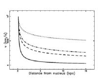
Figure 1.: Classical velocity as a function of the distance from the nucleus when $x_{0}$ =100 pc and $v_{0}=10000\,$km s^-1: $\delta=0$ (full line), $\delta=1$ (dashes), $\delta=1.2$ (dot-dash-dot-dash) and $\delta=1.6$ (dotted).

The rate of mass flow at the point $x$ is

$$\dot{m}(x)=\rho_{{0}}\pi\,x\left(\tan\left(\alpha/2\right)\right)^{2}\sqrt[3]{{x_{{0}}}^{2}\left(\left({\frac{x_{{0}}}{x}}\right)^{\delta}\right)^{2}x}v_{{0}}$$ (24)

and the astrophysical version is

$$\dot{m}(x)=0.02375\,nx\left(\tan\left(\alpha/2\right)\right)^{2}\sqrt[3]{{x_{{0}}}^{2}\left(\left(1.0\,{\frac{x_{{0}}}{x}}\right)^{\delta}\right)^{2}x}\beta_{{0}}{\it Msun}$$ (25)

where $n_{0}$ is the number density of protons expressed in particles cm^-3 at $x_{0}$.

2.4. The Lane–Emden Profile

The self-gravitating sphere of a polytropic gas is governed by the Lane–Emden differential equation of the second order

$${\frac{d^{2}}{d{x}^{2}}}Y(x)+2\,{\frac{{\frac{d}{dx}}Y(x)}{x}}+(Y(x))^{n}=0\quad,$$

where $n$ is an integer, see [15, 16, 17, 18, 19]. The solution $Y(x)_{n}$ has the density profile

$$\rho=\rho_{c}Y(x)_{n}^{n}\quad,$$

where $\rho_{c}$ is the density at $x=0$. The pressure $P$ and temperature $T$ scale as

$$P=K\rho^{1+\frac{1}{n}}\quad,$$ (26)

$$T=K^{\prime}Y(x)\quad,$$ (27)

where K and K^′ are two constants. For more details, see [20].

Analytical solutions exist for $n=0$, 1, and 5. The analytical solution for $n$=5 is

$$Y(x)={\frac{1}{{(1+\frac{{x}^{2}}{3})^{1/2}}}}\quad,$$

and the density for $n$=5 is

$$\rho(x)=\rho_{c}{\frac{1}{{(1+\frac{{x}^{2}}{3})^{5/2}}}}\quad.$$ (28)

The variable $x$ is non-dimensional and we now introduce the new variable $x=r/b$

$$\rho(r;b)=\rho_{c}{\frac{1}{{(1+\frac{{r}^{2}}{3b^{2}})^{5/2}}}}\quad.$$ (29)

Then, the conservation of the flux of energy is

$$\frac{1}{2}\,{\rho_{{0}}{v(x)}^{3}\pi\,{x}^{2}\left(\tan\left(\frac{\alpha}{2}\right)\right)^{2}\left(1+\frac{1}{3}\,{\frac{{x}^{2}}{{b}^{2}}}\right)^{-5/2}}$$

$$=\frac{1}{2}\,{\rho_{{0}}{v_{{0}}(x_{0})}^{3}\pi\,{x_{{0}}}^{2}\left(\tan\left(\frac{\alpha}{2}\right)\right)^{2}\left(1+\frac{1}{3}\,{\frac{{x_{{0}}}^{2}}{{b}^{2}}}\right)^{-5/2}}\quad,$$ (30)

where $v(x)$ is the velocity at position $x$, $v_{0}(x_{0})$ is the velocity at position $x_{0}$ and $\alpha$ is the opening angle of the jet. This equation is a cubic equation, which has one real root plus two non-real complex conjugate roots. Here, and in the following, we only take the real root into account. The real analytical solution for the velocity without losses is

$$v(x;b,x_{0},v_{0})=\frac{v_{{0}}\left(3\,{b}^{2}+{x}^{2}\right)^{{\frac{5}{6}}}{x_{{0}}}^{{\frac{2}{3}}}}{\left(3\,{b}^{2}+{x_{{0}}}^{2}\right)^{{\frac{5}{6}}}{x}^{{\frac{2}{3}}}}\quad.$$ (31)

The asymptotic expansion of above velocity, $v_{a}$, with respect to the variable $x$, which means $x\rightarrow\infty$, is

$$v_{a}(x;b,x_{0},v_{0})=\frac{v_{{0}}{x_{{0}}}^{{\frac{2}{3}}}\left(5\,{b}^{2}+2\,{x}^{2}\right)}{2\,\left(3\,{b}^{2}+{x_{{0}}}^{2}\right)^{5/6}x}\quad.$$ (32)

The trajectory can be found by the indefinite integral of the inverse of the velocity as given by equation (31):

$$F(x)=\int\frac{1}{v(x;b,x_{0},v_{0})}dx=\frac{\sqrt[6]{3}\left(3\,{b}^{2}+{x_{{0}}}^{2}\right)^{{\frac{5}{6}}}{x}^{{\frac{5}{3}}}{\mbox{${}_{2}$F${}_{1}$}({\frac{5}{6}},{\frac{5}{6}};\,{\frac{11}{6}};\,-{\frac{{x}^{2}}{3\,{b}^{2}}})}}{5\,v_{{0}}\left({b}^{2}\right)^{5/6}{x_{{0}}}^{2/3}}\quad,$$ (33)

where ${~{}_{2}F_{1}(a,b;\,c;\,v)}$ is a regularized hypergeometric function, see [21, 22, 23, 24]. The trajectory expressed in terms of $t$ as a function of $x$ is

$$F(x)-F(x_{0})=t\quad.$$ (34)

This equation cannot be inverted in the usual form, which is $x$ as a function of $t$. The asymptotic trajectory can be found by the indefinite integral of the inverse of the asymptotic velocity as given by equation (32)

$$F_{a}(x)=\int\frac{1}{v_{a}(x;b,x_{0},v_{0})}dx=\frac{\left(3\,{b}^{2}+{x_{{0}}}^{2}\right)^{{\frac{5}{6}}}\ln\left(5\,{b}^{2}+2\,{x}^{2}\right)}{2\,v_{{0}}{x_{{0}}}^{2/3}}\quad.$$ (35)

The equation of the asymptotic trajectory is

$$F_{a}(x)-F_{a}(x_{0})=t\quad,$$ (36)

and the solution for $x$ of the above equation, the asymptotic trajectory, is

$$x(t;b,x_{0},v_{0})=\frac{1}{2}\sqrt{-10\,{b}^{2}+2\,{{\rm e}^{{\frac{\left(3\,{b}^{2}+{x_{{0}}}^{2}\right)^{5/6}\ln\left(5\,{b}^{2}+2\,{x_{{0}}}^{2}\right)+2\,tv_{{0}}{x_{{0}}}^{2/3}}{\left(3\,{b}^{2}+{x_{{0}}}^{2}\right)^{5/6}}}}}}\quad.$$ (37)

Figure 2.4. shows a typical example of the above asymptotic expansion.

Table 1.: Parameters for a classical extra-galactic jet

parameter	value
$x_{0}$ (pc)	100
$v_{0}$ ($\frac{km}{s}$)	10000
$b$ (pc)	10000

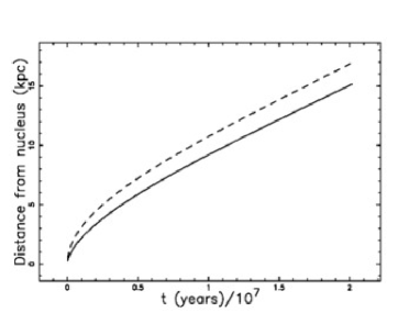
Figure 2.: The numerical solution for a Lane–Emden profile as given by equation (34) (full line) and asymptotic solution as given by equation (37) (dashed line), with parameters as in Table 2.4..

2.5. Solution to Second Order for the Lane–Emden Profile

Let us suppose that the radiative losses in the case of a Lane–Emden profile are proportional to the flux of energy

$$-\epsilon\frac{\rho_{{0}}{v}^{3}\pi\,{x}^{2}\left(\tan\left({\frac{\alpha}{2}}\right)\right)^{2}}{2\,\left(1+\frac{1}{3}\,{\frac{{x}^{2}}{{b}^{2}}}\right)^{5/2}}\quad.$$ (38)

By inserting in the above equation the velocity to first order as given by equation (31), the radiative losses, $Q(x;x_{0},v_{0},b,\epsilon)$, are

$$Q(x;x_{0},v_{0},b,\epsilon)=-\epsilon\frac{\rho_{{0}}{v}^{3}\pi\,{x}^{2}\left(\tan\left({\frac{\alpha}{2}}\right)\right)^{2}}{2\,\left(1+\frac{1}{3}\,{\frac{{x}^{2}}{{b}^{2}}}\right)^{5/2}}\quad,$$ (39)

where $\epsilon$ is a constant which fixes the conversion of the flux of energy to other kinds of energies; in this case, the radiative losses. The sum of the radiative losses between $x_{0}$ and $x$ is given by the following integral, $L$,

$$L(x;x_{0},v_{0},b,\epsilon)=\int_{x_{0}}^{x}Q(x;x_{0},v_{0},b,\epsilon)dx=\frac{-9\,\epsilon\,\rho_{{0}}\sqrt{3}{b}^{5}{v_{{0}}}^{3}{x_{{0}}}^{2}\pi\,\left(\tan\left(\alpha/2\right)\right)^{2}\left(x-x_{{0}}\right)}{2\,\left(3\,{b}^{2}+{x_{{0}}}^{2}\right)^{5/2}}.$$ (40)

The conservation of the flux of energy in the presence of the back-reaction due to the radiative losses for the Lane–Emden profile is

$$\frac{9\,\sqrt{3}\rho_{{0}}\left({b}^{5}{v_{{0}}}^{3}{x_{{0}}}^{2}\epsilon\,\left({\frac{3\,{b}^{2}+{x}^{2}}{{b}^{2}}}\right)^{5/2}x-{b}^{5}{v_{{0}}}^{3}{x_{{0}}}^{3}\epsilon\,\left({\frac{3\,{b}^{2}+{x}^{2}}{{b}^{2}}}\right)^{5/2}+{v}^{3}{x}^{2}\left(3\,{b}^{2}+{x_{{0}}}^{2}\right)^{5/2}\right)}{2\,\left({\frac{3\,{b}^{2}+{x}^{2}}{{b}^{2}}}\right)^{5/2}\left(3\,{b}^{2}+{x_{{0}}}^{2}\right)^{5/2}}$$

$$={9\,\rho_{{0}}\sqrt{3}{v_{{0}}}^{3}{x_{{0}}}^{2}}{2\,\left({\frac{3\,{b}^{2}+{x_{{0}}}^{2}}{{b}^{2}}}\right)^{5/2}}.$$ (41)

The analytical solution for the velocity to second order, $v_{c}(x;b,x_{0},v_{0})$, for the Lane–Emden profile is

$$v_{c}(x;b,x_{0},v_{0})=\frac{v_{{0}}\sqrt[3]{1+\epsilon\,\left(-x+x_{{0}}\right)}\left(3\,{b}^{2}+{x}^{2}\right)^{{\frac{5}{6}}}{x_{{0}}}^{{\frac{2}{3}}}}{\left(3\,{b}^{2}+{x_{{0}}}^{2}\right)^{{\frac{5}{6}}}{x}^{{\frac{2}{3}}}}\quad,$$ (42)

and Figure 2.5. shows an example.

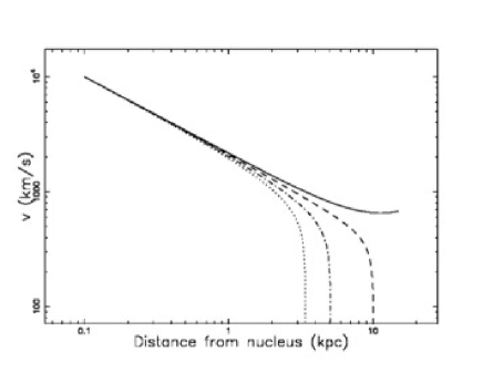
Figure 3.: Velocity corrected for radiative losses for the Lane–Emden profile, i.e., velocity to second order, equation (42), as a function of the distance, with parameters as in Table 2.4.: $\epsilon=0$ full line, $\epsilon=1.0\,10^{-4}$ dashed line, $\epsilon=2.0\,10^{-4}$ dot-dash-dot-dash line and $\epsilon=3.0\,10^{-4}$ dotted line.

There are no analytical results for the trajectory corrected for radiative losses for the Lane–Emden profile, a numerical example is shown in Figure 2.5..

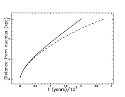
Figure 4.: Numerical trajectory for a Lane–Emden profile corrected for radiative losses as a function of time, with parameters as in Table 2.4.: $\epsilon=0$ full line and $\epsilon=8.0\,10^{-5}$ dashed line.

The inclusion of back-reaction allows the evaluation of the jet’s length, which can be derived from the minimum in the corrected velocity to second order as a function of $x$,

$$\frac{\partial v_{c}(x;b,x_{0},v_{0})}{\partial x}=0\quad,$$ (43)

which is

$$-{\frac{v_{{0}}\epsilon}{3}\left(3\,{b}^{2}+{x}^{2}\right)^{{\frac{5}{6}}}{x_{{0}}}^{{\frac{2}{3}}}\left(1+\epsilon\,\left(-x+x_{{0}}\right)\right)^{-{\frac{2}{3}}}\left(3\,{b}^{2}+{x_{{0}}}^{2}\right)^{-{\frac{5}{6}}}{x}^{-{\frac{2}{3}}}}$$

$$+{\frac{5\,v_{{0}}}{3}\sqrt[3]{1+\epsilon\,\left(-x+x_{{0}}\right)}{x_{{0}}}^{{\frac{2}{3}}}\sqrt[3]{x}\left(3\,{b}^{2}+{x_{{0}}}^{2}\right)^{-{\frac{5}{6}}}{\frac{1}{\sqrt[6]{3\,{b}^{2}+{x}^{2}}}}}$$

$$-{\frac{2\,v_{{0}}}{3}\sqrt[3]{1+\epsilon\,\left(-x+x_{{0}}\right)}\left(3\,{b}^{2}+{x}^{2}\right)^{{\frac{5}{6}}}{x_{{0}}}^{{\frac{2}{3}}}\left(3\,{b}^{2}+{x_{{0}}}^{2}\right)^{-{\frac{5}{6}}}{x}^{-{\frac{5}{3}}}}=0\quad.$$ (44)

The solution for $x$ of the above minimum determines the jet’s length, $x_{j}$,

$$x_{j}=\frac{4\,{b}^{2}{\epsilon}^{2}+{\epsilon}^{2}{x_{{0}}}^{2}+\sqrt[3]{D_{{2}}}\epsilon\,x_{{0}}+{D_{{2}}}^{{\frac{2}{3}}}+2\,\epsilon\,x_{{0}}+\sqrt[3]{D_{{2}}}+1}{4\,\epsilon\,\sqrt[3]{D_{{2}}}}\quad,$$ (45)

where

$$D_{1}=-16\,{b}^{4}{\epsilon}^{4}+429\,{b}^{2}{\epsilon}^{4}{x_{{0}}}^{2}-24\,{\epsilon}^{4}{x_{{0}}}^{4}+858\,{b}^{2}{\epsilon}^{3}x_{{0}}$$

$$-96\,{\epsilon}^{3}{x_{{0}}}^{3}+429\,{b}^{2}{\epsilon}^{2}-144\,{\epsilon}^{2}{x_{{0}}}^{2}-96\,\epsilon\,x_{{0}}-24\quad,$$ (46)

and

$$D_{2}=-42\,{b}^{2}{\epsilon}^{3}x_{{0}}+{\epsilon}^{3}{x_{{0}}}^{3}-42\,{b}^{2}{\epsilon}^{2}+3\,{\epsilon}^{2}{x_{{0}}}^{2}+2\,b\sqrt{{\it D1}}\epsilon+3\,\epsilon\,x_{{0}}+1\quad.$$ (47)

Figure 2.5. shows $x_{j}$ numerically.

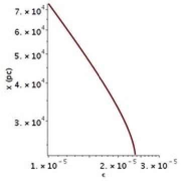
Figure 5.: Length of the jet for a Lane–Emden profile, $x_{j}$, in pc as a function of $\epsilon$, with $b$ as in Table 2.4..

3. Relativistic Turbulent Jets

The conservation of the energy flux in special relativity (SR) in the presence of a velocity $v$ along one direction states that

$$A(x)\frac{1}{1-\frac{v^{2}}{c^{2}}}(e_{0}+p_{0})v=cost$$ (48)

where

$$A(x)=\pi(x\tan(\frac{\alpha}{2}))^{2}\quad,$$ (49)

is the considered area in the direction perpendicular to the motion, $c$ is the speed of light, $e_{0}=c^{2}\rho$ is the energy density in the rest frame of the moving fluid, and $p_{0}$ is the pressure in the rest frame of the moving fluid, see formula A31 in [10]. In accordance with the current models of classical turbulent jets, we insert $p_{0}=0$ and the conservation law for relativistic energy flux is

$$\rho c^{2}v\frac{1}{1-\frac{v^{2}}{c^{2}}}A(x)=cost\quad.$$ (50)

Our physical units are pc for length and yr for time, and in these units, the speed of light is $c=0.306$  pc  yr^-1. A discussion of the mass–energy equivalence principle in fluids can be found in [25].

3.1. Constant Density in SR

The conservation of the relativistic energy flux when the density is constant can be written as a differential equation

$${\rho\,{c}^{2}\left({\frac{\rm d}{{\rm d}t}}x\left(t\right)\right)\pi\,\left(x\left(t\right)\right)^{2}\left(\tan\left(\frac{\alpha}{2}\right)\right)^{2}\left(1-{\frac{\left({\frac{\rm d}{{\rm d}t}}x\left(t\right)\right)^{2}}{{c}^{2}}}\right)^{-1}}$$

$$-{\rho\,{c}^{2}v_{{0}}\pi\,{x_{{0}}}^{2}\left(\tan\left(\frac{\alpha}{2}\right)\right)^{2}\left(1-{\frac{{v_{{0}}}^{2}}{{c}^{2}}}\right)^{-1}}=0\quad.$$ (51)

Although an analytical solution of the previous differential equation at the moment of writing does not exist, we can provide a power series solution of the form

$$x(t)=a_{0}+a_{1}t+a_{2}t^{2}+a_{3}t^{3}+\dots$$ (52)

see [26, 27]. The coefficients $a_{n}$ up to order 4 are

$$a_{0}= x_{{0}}$$

$$a_{1}= v_{{0}}$$

$$a_{2}= \frac{1}{3}\,{\frac{{v_{{0}}}^{3}\left(5\,{c}^{6}-11\,{c}^{4}{v_{{0}}}^{2}+3\,{c}^{2}{v_{{0}}}^{4}+3\,{v_{{0}}}^{6}\right)}{{x_{{0}}}^{2}\left({c}^{2}+{v_{{0}}}^{2}\right)\left({c}^{4}+2\,{c}^{2}{v_{{0}}}^{2}+{v_{{0}}}^{4}\right)}}$$

$$a_{3}= \frac{1}{3}\,{\frac{{v_{{0}}}^{3}\left(5\,{c}^{6}-11\,{c}^{4}{v_{{0}}}^{2}+3\,{c}^{2}{v_{{0}}}^{4}+3\,{v_{{0}}}^{6}\right)}{{x_{{0}}}^{2}\left({c}^{2}+{v_{{0}}}^{2}\right)\left({c}^{4}+2\,{c}^{2}{v_{{0}}}^{2}+{v_{{0}}}^{4}\right)}}\quad.$$ (53)

To find a numerical solution of this differential equation, we isolate the velocity from Eq. (51)

$$v(x;x_{0},\beta_{0},c)=$$

$$\frac{1}{2}\,{\frac{\left({\beta_{{0}}}^{2}{x}^{2}-{x}^{2}+\sqrt{{x}^{4}{\beta_{{0}}}^{4}-2\,{x}^{4}{\beta_{{0}}}^{2}+4\,{\beta_{{0}}}^{2}{x_{{0}}}^{4}+{x}^{4}}\right)c}{\beta_{{0}}{x_{{0}}}^{2}}}\,$$ (54)

where $\beta_{0}=\frac{v_{0}}{c}$ and separate the variables

$$\int_{x_{0}}^{x}2\,{\frac{\beta_{{0}}{x_{{0}}}^{2}}{\left({\beta_{{0}}}^{2}{x}^{2}-{x}^{2}+\sqrt{{x}^{4}{\beta_{{0}}}^{4}-2\,{x}^{4}{\beta_{{0}}}^{2}+4\,{\beta_{{0}}}^{2}{x_{{0}}}^{4}+{x}^{4}}\right)c}}dx$$

$$=\int_{0}^{t}dt\quad.$$ (55)

The indefinite integral on the left side of the previous equation has an analytical expression

$$I(x;\beta_{0},c,x_{0})=\frac{AN}{AD}$$ (56)

where

$$AN=$$

$$2\,{\beta_{{0}}}^{3}{x_{{0}}}^{6}\sqrt{2}\sqrt{4-2\,{\frac{i\beta_{{0}}{x}^{2}}{{x_{{0}}}^{2}}}+2\,{\frac{i{x}^{2}}{\beta_{{0}}{x_{{0}}}^{2}}}}\sqrt{4+2\,{\frac{i\beta_{{0}}{x}^{2}}{{x_{{0}}}^{2}}}-2\,{\frac{i{x}^{2}}{\beta_{{0}}{x_{{0}}}^{2}}}}\times~{}$$

$$\times{\it F}(1/2\,x\sqrt{2}\sqrt{{\frac{i({\beta_{{0}}}^{2}-1)}{\beta_{{0}}{x_{{0}}}^{2}}}},i)$$

$$-{\beta_{{0}}}^{3}{x_{{0}}}^{2}{x}^{3}\sqrt{{\frac{i\beta_{{0}}}{{x_{{0}}}^{2}}}-{\frac{i}{\beta_{{0}}{x_{{0}}}^{2}}}}\sqrt{{x}^{4}{\beta_{{0}}}^{4}-2\,{x}^{4}{\beta_{{0}}}^{2}+4\,{\beta_{{0}}}^{2}{x_{{0}}}^{4}+{x}^{4}}~{}$$

$$+\beta_{{0}}{x_{{0}}}^{2}{x}^{3}\sqrt{{\frac{i\beta_{{0}}}{{x_{{0}}}^{2}}}-{\frac{i}{\beta_{{0}}{x_{{0}}}^{2}}}}\sqrt{{x}^{4}{\beta_{{0}}}^{4}-2\,{x}^{4}{\beta_{{0}}}^{2}+4\,{\beta_{{0}}}^{2}{x_{{0}}}^{4}+{x}^{4}}$$

$$+{\beta_{{0}}}^{5}{x_{{0}}}^{2}{x}^{5}\sqrt{{\frac{i\beta_{{0}}}{{x_{{0}}}^{2}}}-{\frac{i}{\beta_{{0}}{x_{{0}}}^{2}}}}-2\,{\beta_{{0}}}^{3}{x_{{0}}}^{2}{x}^{5}\sqrt{{\frac{i\beta_{{0}}}{{x_{{0}}}^{2}}}-{\frac{i}{\beta_{{0}}{x_{{0}}}^{2}}}}~{}$$

$$+4\,{\beta_{{0}}}^{3}{x_{{0}}}^{6}x\sqrt{{\frac{i\beta_{{0}}}{{x_{{0}}}^{2}}}-{\frac{i}{\beta_{{0}}{x_{{0}}}^{2}}}}+\beta_{{0}}{x_{{0}}}^{2}{x}^{5}\sqrt{{\frac{i\beta_{{0}}}{{x_{{0}}}^{2}}}-{\frac{i}{\beta_{{0}}{x_{{0}}}^{2}}}}$$ (57)

and

$$AD=$$

$$6\,c{\beta_{{0}}}^{2}{x_{{0}}}^{4}\sqrt{{\frac{i\beta_{{0}}}{{x_{{0}}}^{2}}}-{\frac{i}{\beta_{{0}}{x_{{0}}}^{2}}}}\sqrt{{x}^{4}{\beta_{{0}}}^{4}-2\,{x}^{4}{\beta_{{0}}}^{2}+4\,{\beta_{{0}}}^{2}{x_{{0}}}^{4}+{x}^{4}}$$ (58)

where $i=\sqrt{-1}$ and

$$F(x;m)=\int_{0}^{x}\!{\frac{1}{\sqrt{1-{{\it t}}^{2}}\sqrt{1-{m}^{2}{{\it t}}^{2}}}}\,{\rm d}{\it t}$$ (59)

is the elliptic integral of the first kind, see formula 17.2.7 in [21]. Figure 3.1. shows the behaviour of $\beta$ as function of the distance.

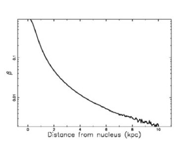
Figure 6.: Relativistic $\beta$ for constant density as a function of the distance from the nucleus when $x_{0}$ =200 pc and $\beta_{0}$ =0.9 in the case of constant density.

A numerical solution can be found by solving the following non-linear equation

$$I(x;\beta_{0},c,x_{0})-I(x_{0};\beta_{0},c,x_{0})=t$$ (60)

and Figure 3.1. presents a typical comparison with the series solution.

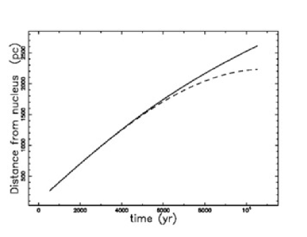
Figure 7.: Non-linear relativistic solution for constant density as given by Eq. (60) (full line) and series solution as given by Eq. (52) (dashed line) when $x_{0}$ =100 pc and $\beta_{0}$ =0.999.

The relativistic rate of mass flow in the case of constant density is

$$\dot{m}(x)=$$

$$\frac{\rho\,\left({\beta_{{0}}}^{2}{x}^{2}-{x}^{2}+\sqrt{{x}^{4}{\beta_{{0}}}^{4}-2\,{x}^{4}{\beta_{{0}}}^{2}+4\,{\beta_{{0}}}^{2}{x_{{0}}}^{4}+{x}^{4}}\right)c\pi\,x\left(\tan\left(\alpha/2\right)\right)^{2}}{\sqrt{2\left(1-{\beta_{{0}}}^{2}\right)\left({\beta_{{0}}}^{2}{x}^{2}-{x}^{2}+\sqrt{{x}^{4}{\beta_{{0}}}^{4}-2\,{x}^{4}{\beta_{{0}}}^{2}+4\,{\beta_{{0}}}^{2}{x_{{0}}}^{4}+{x}^{4}}\right)}}$$ (61)

3.2. Inverse Power Law Profile of Density in SR

The conservation of the relativistic energy flux in the presence of an inverse power law density profile as given by Eq. (21) is

$${\rho_{0}\,{c}^{2}\left({\frac{\rm d}{{\rm d}t}}x\left(t\right)\right)\pi\,\left(x\left(t\right)\right)^{2}\left(\tan\left(\frac{\alpha}{2}\right)\right)^{2}\left({\frac{x_{{0}}}{x\left(t\right)}}\right)^{\delta}\left(-{\frac{\left({\frac{\rm d}{{\rm d}t}}x\left(t\right)\right)^{2}}{{c}^{2}}}+1\right)^{-1}}$$

$$-{\rho_{0}\,{c}^{2}v_{{0}}\pi\,{x_{{0}}}^{2}\left(\tan\left(\frac{\alpha}{2}\right)\right)^{2}\left(-{\frac{{v_{{0}}}^{2}}{{c}^{2}}}+1\right)^{-1}}=0\quad.$$ (62)

This differential equation does not have an analytical solution. An expression for $\beta$ as a function of the distance is

$$\beta(x)=\frac{1}{2}\,{\frac{1}{\beta_{{0}}{x_{{0}}}^{2}}\left({\beta_{{0}}}^{2}{x}^{2}\left({\frac{x_{{0}}}{x}}\right)^{\delta}-{x}^{2}\left({\frac{x_{{0}}}{x}}\right)^{\delta}+\sqrt{D}\right)}$$ (63)

with

$$D= \left(\left({\frac{x_{{0}}}{x}}\right)^{\delta}\right)^{2}{\beta_{{0}}}^{4}{x}^{4}-2\,\left(\left({\frac{x_{{0}}}{x}}\right)^{\delta}\right)^{2}{\beta_{{0}}}^{2}{x}^{4}+\left(\left({\frac{x_{{0}}}{x}}\right)^{\delta}\right)^{2}{x}^{4}+4\,{\beta_{{0}}}^{2}{x_{{0}}}^{4}.$$ (64)

The behaviour of $\beta$ as a function of the distance for different values of $\delta$ can be seen in Figure 3.2..

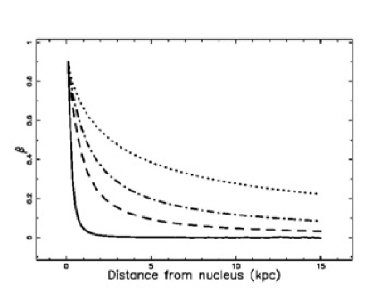
Figure 8.: Relativistic $\beta$ for the relativistic energy flux conservation in the presence of an inverse power law as a function of the distance from the nucleus when $x_{0}$ =100 pc and $\beta_{0}$ =0.9: $\delta=0$ (full line), $\delta=1$ (dashes), $\delta=1.2$ (dot-dash-dot-dash) and $\delta=1.4$ (dotted).

A power series solution for this differential equation (62) up to order three gives

$$a_{0}= x_{{0}}$$

$$a_{1}= v_{{0}}$$

$$a_{2}= \frac{1}{2}\,{\frac{{v_{{0}}}^{2}\left({c}^{2}\delta-\delta\,{v_{{0}}}^{2}-2\,{c}^{2}+2\,{v_{{0}}}^{2}\right)}{x_{{0}}\left({c}^{2}+{v_{{0}}}^{2}\right)}}\quad.$$ (65)

Figure 3.2. shows a comparison between the numerical solution of (62) with the series solution.

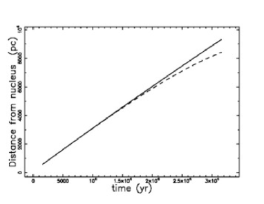
Figure 9.: Non-linear relativistic solution in presence of an inverse power law as given by Eq. (62) (full line) and series solution as given by Eq. (65) (dashed line) when $x_{0}$ =100 pc and $\beta_{0}$ =0.999.

The relativistic rate of mass flow in the case of an inverse power law for the density is

$$\dot{m}(x)=\frac{\rho_{{0}}\left({\frac{x_{{0}}}{x}}\right)^{\delta}\left({\beta_{{0}}}^{2}{x}^{2}\left({\frac{x_{{0}}}{x}}\right)^{\delta}-{x}^{2}\left({\frac{x_{{0}}}{x}}\right)^{\delta}+\sqrt{D}\right)c\pi\,{x}^{2}\left(\tan\left(\alpha/2\right)\right)^{2}}{2\,\beta_{{0}}{x_{{0}}}^{2}\sqrt{-1/4\,{\frac{1}{{\beta_{{0}}}^{2}{x_{{0}}}^{4}}\left({\beta_{{0}}}^{2}{x}^{2}\left({\frac{x_{{0}}}{x}}\right)^{\delta}-{x}^{2}\left({\frac{x_{{0}}}{x}}\right)^{\delta}+\sqrt{D}\right)^{2}}+1}}$$ (66)

where $\rho_{0}$ is the density at $x_{0}$ and $D$ was defined in Eq. (64).

3.3. The Lane–Emden Profile

In the presence of a Lane–Emden ($n=5$) density profile, as given by equation (29) and $A(x)$ as given by equation (49), the conservation of relativistic flux of energy for a straight jet takes the form

$$\frac{\rho_{{0}}{c}^{3}\beta\,\pi\,{x}^{2}\left(\tan\left(\alpha/2\right)\right)^{2}}{\left(1+\frac{1}{3}\,{\frac{{x}^{2}}{{b}^{2}}}\right)^{5/2}\left(1-{\beta}^{2}\right)}=\frac{\rho_{{0}}{c}^{3}\beta 0\,\pi\,{x_{{0}}}^{2}\left(\tan\left(\alpha/2\right)\right)^{2}}{\left(1+\frac{1}{3}\,{\frac{{x_{{0}}}^{2}}{{b}^{2}}}\right)^{5/2}\left({1-\beta 0}^{2}\right)},$$ (67)

where $v$ is the velocity at $x$, $v_{0}$ is the velocity at $x_{0}$, $\beta=\frac{v}{c}$ and $\beta_{0}=\frac{v_{0}}{c}$. The solution for $\beta$ to first order is

$$\beta(x;x_{0},b,\beta_{0})=\frac{N}{\left(1+\frac{1}{3}\,{\frac{{x_{{0}}}^{2}}{{b}^{2}}}\right)^{5/2}\left({\beta 0}^{2}-1\right)},$$ (68)

where

$$N=9\,\sqrt{3\,{b}^{2}+{x_{{0}}}^{2}}{x}^{2}{b}^{4}{\beta_{{0}}}^{2}+6\,\sqrt{3\,{b}^{2}+{x_{{0}}}^{2}}{x}^{2}{b}^{2}{x_{{0}}}^{2}{\beta_{{0}}}^{2}+\sqrt{3\,{b}^{2}+{x_{{0}}}^{2}}{x}^{2}{x_{{0}}}^{4}{\beta_{{0}}}^{2}$$

$$-9\,\sqrt{3\,{b}^{2}+{x_{{0}}}^{2}}{x}^{2}{b}^{4}-6\,\sqrt{3\,{b}^{2}+{x_{{0}}}^{2}}{x}^{2}{b}^{2}{x_{{0}}}^{2}-\sqrt{3\,{b}^{2}+{x_{{0}}}^{2}}{x}^{2}{x_{{0}}}^{4}$$

$$+\Biggl{(}243\,{x}^{4}({b}^{2}+\frac{1}{3}\,{x_{{0}}}^{2})^{5}{\beta_{{0}}}^{4}+(-2\,{x}^{4}{x_{{0}}}^{10}-30\,{b}^{2}{x}^{4}{x_{{0}}}^{8}-180\,{b}^{4}{x}^{4}{x_{{0}}}^{6}$$

$$+(972\,{b}^{10}+1620\,{b}^{8}{x}^{2}+540\,{b}^{6}{x}^{4}+360\,{b}^{4}{x}^{6}+60\,{b}^{2}{x}^{8}+4\,{x}^{10}){x_{{0}}}^{4}$$

$$-810\,{b}^{8}{x}^{4}{x_{{0}}}^{2}-486\,{b}^{10}{x}^{4}){\beta_{{0}}}^{2}+243\,{x}^{4}({b}^{2}+\frac{1}{3}\,{x_{{0}}}^{2})^{5}\Biggr{)}^{1/2}.$$ (69)

The equation for the relativistic trajectory is

$$\int_{x_{0}}^{x}\frac{1}{\beta(x;x_{0},b,\beta_{0})\,c}dx=t\quad.$$ (70)

The integral in this equation does not have an analytical solution and should be integrated numerically. To have analytical results, two approximations are now introduced. The first approximation computes a truncated series expansion for the integrand of the integral in equation (70), which transforms the relativistic equation of motion into

$$F(x)-F(x_{0})=t\quad,$$ (71)

with

$$F(x)=\frac{NF}{162\,{x_{{0}}}^{2}\beta_{{0}}{b}^{10}c}\quad,$$ (72)

where

$$NF=\left({b}^{2}\right)^{5/2}x\Bigl{(}9\,\sqrt{3}\sqrt{3\,{b}^{2}+{x_{{0}}}^{2}}{b}^{4}{\beta_{{0}}}^{2}{x}^{2}+6\,\sqrt{3}\sqrt{3\,{b}^{2}+{x_{{0}}}^{2}}{b}^{2}{\beta_{{0}}}^{2}{x}^{2}{x_{{0}}}^{2}$$

$$+\sqrt{3}\sqrt{3\,{b}^{2}+{x_{{0}}}^{2}}{\beta_{{0}}}^{2}{x}^{2}{x_{{0}}}^{4}-9\,\sqrt{3}\sqrt{3\,{b}^{2}+{x_{{0}}}^{2}}{b}^{4}{x}^{2}$$

$$-6\,\sqrt{3}\sqrt{3\,{b}^{2}+{x_{{0}}}^{2}}{b}^{2}{x}^{2}{x_{{0}}}^{2}-\sqrt{3}\sqrt{3\,{b}^{2}+{x_{{0}}}^{2}}{x}^{2}{x_{{0}}}^{4}-162\,\sqrt{{b}^{10}{x_{{0}}}^{4}{\beta_{{0}}}^{2}}\Bigr{)}.$$ (73)

In this analytical result we have time as a function of the distance, see Figure 3.3. where the percentage error at $x=15$ kpc is $\delta=15.91\%$.

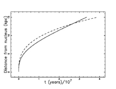
Figure 10.: Numerical relativistic solution for a Lane–Emden ($n=5$) density profile as given by equation (70) (full line) and truncated series expansion as given by equation (3.3.) (dashed line), with parameters as in Table 3.3..

Table 2.: Parameters for a relativistic extra-galactic jet.

parameter	value
$x_{0}$ (pc)	100
$\beta_{0}$	0.9
$b$ (pc)	10000

The second approximation computes a Padé approximant of order [2/1], see [28, 29, 30], for the integrand of the integral in equation (70)

$$P(x)-P(x_{0})=t\quad,$$ (74)

with

$$P(x)\frac{NP}{162\,{b}^{10}{x_{{0}}}^{4}{\beta_{{0}}}^{2}c}\quad,$$ (75)

where

$$NP(x)=-x\left({b}^{2}\right)^{5/2}{x_{{0}}}^{2}\beta_{{0}}\Big{(}9\,\sqrt{3}\sqrt{3\,{b}^{2}+{x_{{0}}}^{2}}{b}^{4}{\beta_{{0}}}^{2}{x}^{2}$$

$$+6\,\sqrt{3}\sqrt{3\,{b}^{2}+{x_{{0}}}^{2}}{b}^{2}{\beta_{{0}}}^{2}{x}^{2}{x_{{0}}}^{2}+\sqrt{3}\sqrt{3\,{b}^{2}+{x_{{0}}}^{2}}{\beta_{{0}}}^{2}{x}^{2}{x_{{0}}}^{4}$$

$$-9\,\sqrt{3}\sqrt{3\,{b}^{2}+{x_{{0}}}^{2}}{b}^{4}{x}^{2}-6\,\sqrt{3}\sqrt{3\,{b}^{2}+{x_{{0}}}^{2}}{b}^{2}{x}^{2}{x_{{0}}}^{2}-\sqrt{3}\sqrt{3\,{b}^{2}+{x_{{0}}}^{2}}{x}^{2}{x_{{0}}}^{4}$$

$$-162\,\sqrt{{b}^{10}{x_{{0}}}^{4}{\beta_{{0}}}^{2}}\Big{)}.$$ (76)

Although this equation can be inverted, the analytical expression for $x=G(t;x_{0},\beta_{0},b)$ as a function of time is complicated and is consequently omitted here. As an example, with the parameters of Table 3.3., we have

$$G(t)=\frac{NG}{DG}\quad,$$ (77)

with

$$NG=-{2.9237\times 10^{-17}}\,\Bigl{(}-{1.7397\times 10^{54}}\,t-{5.8851\times 10^{56}}$$

$$+{2.9816\times 10^{20}}\,\sqrt{{1.9201\times 10^{73}}+{2.3032\times 10^{70}}\,t}$$

$${+{3.4042\times 10^{67}}\,{t}^{2}}\Bigr{)}^{2/3}+{3.2399\times 10^{21}}\quad,$$ (78)

and

$$DG=\Bigg{(}-{1.7397\times 10^{54}}\,t-{5.8851\times 10^{56}}$$

$$+{2.9816\times 10^{20}}\,\sqrt{{1.9201\times 10^{73}}+{2.3032\times 10^{70}}\,t+{3.4042\times 10^{67}}\,{t}^{2}}\Bigg{)}^{\frac{1}{3}}.$$ (79)

An example is shown in Figure 3.3., where the percentage error at $x=15$ kpc is $\delta=4.81\%$.

Figure 11.: Numerical relativistic solution for a Lane–Emden ($n=5$) density profile as given by equation (70) (full line) and Padé approximant as given by equation (3.3.) (dashed line), with parameters as in Table 3.3..

3.4. Relativistic Solution to Second Order

We now suppose that the radiative losses for a Lane–Emden ($n=5$) density profile are proportional to the relativistic flux of energy. The integral of the losses, $L_{r}$, between $x_{0}$ and $x$ is

$$L_{r}(x;x_{0},\beta_{0},b,c)=-\epsilon\frac{9\,\left(x-x_{{0}}\right)\rho 0\,{c}^{3}\beta_{{0}}{x_{{0}}}^{2}\pi\,\left(\tan\left(\alpha/2\right)\right)^{2}{b}^{5}\sqrt{3}}{\left(3\,{b}^{2}+{x_{{0}}}^{2}\right)^{5/2}\left(1-{\beta_{{0}}}^{2}\right)}\quad.$$ (80)

The conservation of the relativistic flux of energy in the presence of the back-reaction due to the radiative losses is

$$\frac{NR}{\left(3\,{b}^{2}+{x}^{2}\right)^{5/2}\left(3\,{b}^{2}+{x_{{0}}}^{2}\right)^{5/2}\left({\beta}^{2}-1\right)\left({\beta_{{0}}}^{2}-1\right)}=$$

$$\frac{9\,\rho 0\,\sqrt{3}{c}^{3}\beta_{{0}}{x_{{0}}}^{2}{b}^{5}}{\left(3\,{b}^{2}+{x_{{0}}}^{2}\right)^{5/2}\left({\beta_{{0}}}^{2}-1\right)}\quad,$$ (81)

where

$$NR=81\,\rho 0\,{b}^{5}\sqrt{3}\Bigg{(}({b}^{2}+\frac{1}{3}\,{x}^{2})^{2}\epsilon\,(\beta+1)\beta_{{0}}(\beta-1)(x-x_{{0}}){x_{{0}}}^{2}\sqrt{3\,{b}^{2}+{x}^{2}}$$

$$+({b}^{2}+\frac{1}{3}\,{x_{{0}}}^{2})^{2}\beta\,{x}^{2}(\beta_{{0}}+1)(\beta_{{0}}-1)\sqrt{3\,{b}^{2}+{x_{{0}}}^{2}}\Bigg{)}{c}^{3}.$$ (82)

The solution of this equation, to second order, for $\beta$ is

$$\beta=\frac{NB}{2\,\left(3\,{b}^{2}+{x}^{2}\right)^{5/2}\left(\epsilon\,x-\epsilon\,x_{{0}}-1\right)\left(3\,{b}^{2}+{x_{{0}}}^{2}\right){x_{{0}}}^{2}\beta_{{0}}}\quad,$$ (83)

where

$$NB=-\sqrt{3\,{b}^{2}+{x_{{0}}}^{2}}\Bigg{(}\sqrt{3\,{b}^{2}+{x_{{0}}}^{2}}\times$$

$$\Big{(}{{x}^{4}(\beta_{{0}}-1)^{2}(\beta_{{0}}+1)^{2}{x_{{0}}}^{10}+15\,{b}^{2}{x}^{4}(\beta_{{0}}-1)^{2}(\beta_{{0}}+1)^{2}{x_{{0}}}^{8}}$$

$${+(972\,({b}^{2}+\frac{1}{3}\,{x}^{2})^{5}{\beta_{{0}}}^{2}{\epsilon}^{2}+90\,{b}^{4}{x}^{4}(\beta_{{0}}-1)^{2}(\beta_{{0}}+1)^{2}){x_{{0}}}^{6}}$$

$${-1944\,\epsilon\,({b}^{2}+\frac{1}{3}\,{x}^{2})^{5}{\beta_{{0}}}^{2}(\epsilon\,x-1){x_{{0}}}^{5}+(972\,({b}^{2}+\frac{1}{3}\,{x}^{2})^{5}{\beta_{{0}}}^{2}{x}^{2}{\epsilon}^{2}}$$

$${-1944\,({b}^{2}+\frac{1}{3}\,{x}^{2})^{5}{\beta_{{0}}}^{2}x\epsilon+4\,{x}^{10}{\beta_{{0}}}^{2}+60\,{b}^{2}{x}^{8}{\beta_{{0}}}^{2}+360\,{b}^{4}{x}^{6}{\beta_{{0}}}^{2}}$$

$${+270\,{b}^{6}({\beta_{{0}}}^{2}+1)^{2}{x}^{4}+1620\,{b}^{8}{x}^{2}{\beta_{{0}}}^{2}+972\,{b}^{10}{\beta_{{0}}}^{2}){x_{{0}}}^{4}}$$

$${+405\,{b}^{8}{x}^{4}(\beta_{{0}}-1)^{2}(\beta_{{0}}+1)^{2}{x_{{0}}}^{2}+243\,{b}^{10}{x}^{4}(\beta_{{0}}-1)^{2}(\beta_{{0}}+1)^{2}}\Big{)}^{1/2}$$

$$+27\,({b}^{2}+\frac{1}{3}\,{x_{{0}}}^{2})^{3}(\beta_{{0}}+1){x}^{2}(\beta_{{0}}-1)\Bigg{)}\quad.$$ (84)

The relativistic equation of motion with back-reaction can be solved by numerically integrating the relation in equation (70). Figure 3.4. gives an example.

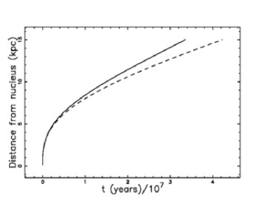
Figure 12.: Numerical relativistic solution for a Lane–Emden ($n=5$) density profile as given by equation (70) (full line) and solution with back-reaction, i.e., to second order, (dashed line), with parameters as in Table 3.3. and $\epsilon=2.0\,10^{-5}$.

4. Astrophysical Applications

We now analyse two models for the synchrotron emission along the jet for a Lane–Emden ($n=5$) density profile.

4.1. Direct Conversion

The flux of observed radiation along the centre of the jet, $I_{c}$, in the classical case is assumed to scale as

$$I_{c}(x;x_{0},v_{0},b,\epsilon)\propto\frac{L(x;x_{0},v_{0},b,\epsilon)}{x^{2}}\quad,$$ (85)

where $L$, the sum of the radiative losses for a Lane–Emden ($n=5$) density profile, is given by equation (40).

This relation connects the observed intensity of radiation with the rate of energy transfer per unit area. In the relativistic case

$$I_{c}(x;x_{0},\beta_{0},b,c)\propto\frac{L_{r}(x;x_{0},\beta_{0},b,c)}{x^{2}}\quad,$$ (86)

where $L_{r}$ is given by equation (80)

The observational percentage of reliability can be used as a statistical test for the the goodness of fit, $\epsilon_{\mathrm{obs}}$,

$$\epsilon_{\mathrm{obs}}=100\bigl{(}1-\frac{\sum_{j}|I_{obs}-I_{theo}|_{j}}{\sum_{j}I_{theo,j}}\bigr{)}.$$ (87)

We now report the large scale structure and jets of 3C31, see Figure 4.1..

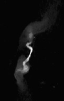
Figure 13.: Extended image (300 kpc) of 3C31.

To make a comparison with the observed profile of intensity, we choose the first 10 kpc of 3C31, see Figures 1 and 8 in [14]; Figure 4.1. shows the theoretical synchrotron intensity, as well as the observed one.

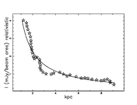
Figure 14.: Observed intensity profile along the centerline of 3C31 (empty stars) and theoretical intensity for a Lane–Emden ($n=5$) density profile as given by equation (86), with parameters as in Table 3.3. (full line). The observational percentage of reliability is $\epsilon_{\mathrm{obs}}=86.19\%$.

4.2. The Magnetic Field of Equipartition

The magnetic field in CGS has an energy density of $\frac{B^{2}}{8\pi}$, where $B$ is the magnetic field. The presence of the magnetic field can be modeled assuming equipartition between the kinetic energy and the magnetic energy

$$\frac{B(x)^{2}}{8\pi}=\frac{1}{2}\rho v^{2}\quad.$$ (88)

By inserting the above equation in the classical equation for the conservation of the flux of energy (4), a factor 2 will appear on both sides of the equation, leaving unchanged the result for the deduction of the velocity to the first order. The magnetic field as a function of the distance $x$ when the velocity is given by equation (31) and in the presence of a Lane–Emden ($n=5$) profile for the density is

$$B(x;x_{0},b)=\frac{B_{{0}}\left(3\,{b}^{2}+{x_{{0}}}^{2}\right)^{{\frac{5}{12}}}{x_{{0}}}^{{\frac{2}{3}}}}{\left(3\,{b}^{2}+{x}^{2}\right)^{{\frac{5}{12}}}{x}^{{\frac{2}{3}}}}\quad.$$ (89)

where $B_{0}$ is the magnetic field at $x=x_{0}$. We assume an inverse power law spectrum for the ultrarelativistic electrons, of the type

$$N(E)dE=KE^{-p}dE$$ (90)

where $K$ is a constant and $p$ the exponent of the inverse power law. The intensity of the synchrotron radiation has a standard expression, as given by formula (1.175) in [31],

$$I(\nu)\approx 0.933\times 10^{-23}\alpha_{p}(p)KlH_{\perp}^{(p+1)/2}\bigl{(}\frac{6.26\times 10^{18}}{\nu}\bigr{)}^{(p-1)/2}$$ (91)

$$erg\,sec^{-1}cm^{-2}Hz^{-1}rad^{-2}$$

where $\nu$ is the frequency, $H_{\perp}$ is the magnetic field perpendicular to the electron’s velocity, $l$ is the dimension of the radiating region along the line of sight, and $\alpha_{p}(p)$ is a slowly varying function of $p$, which is of the order of unity. We now analyse the intensity along the centerline of the jet, which means that the radiating length is

$$l(x;\alpha)=x\tan(\frac{\alpha}{2})\quad.$$ (92)

The intensity, assuming a constant $p$, scales as

$$I(x;x_{0},p)=\frac{I_{{0}}{B}^{{\frac{p}{2}}+{\frac{1}{2}}}x}{{B_{{0}}}^{{\frac{p}{2}}+{\frac{1}{2}}}{\it x_{0}}}\quad,$$ (93)

where $I_{0}$ is the intensity at $x=x_{0}$ and $B_{0}$ the magnetic field at $x=x_{0}$. We insert Eq. (89) to have an analytical expression for the centerline intensity

$$I(x;x_{0},p,b)=\left(3\,{b}^{2}+{x_{{0}}}^{2}\right)^{{\frac{5\,p}{24}}+{\frac{5}{24}}}i_{{0}}{x}^{-{\frac{p}{3}}+{\frac{2}{3}}}{x_{{0}}}^{{\frac{p}{3}}-{\frac{2}{3}}}\left(3\,{b}^{2}+{x}^{2}\right)^{-{\frac{5\,p}{24}}-{\frac{5}{24}}}\quad.$$ (94)

This equation for the intensity is relative to the unit area; to have the intensity on the centerline, $I_{c}$, we should make a further division by the area of interest, which scales $\propto\,x^{2}$

$$I_{c}(x;x_{0},p,b)=\frac{I(x;x_{0},p,b)}{x^{2}}\quad.$$ (95)

Figure 4.2. shows the theoretical synchrotron intensity with the variable magnetic field, as well as the observed one for 3C31.

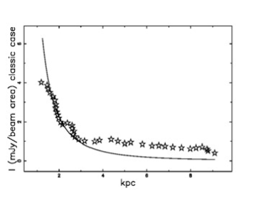
Figure 15.: Observed intensity profile along the centerline, $I_{c}$, of 3C31 (empty stars) and theoretical intensity for a Lane–Emden ($n=5$) density profile as given by equation (95), with parameters as in Table 2.4.. The observational percentage of reliability is $\epsilon_{\mathrm{obs}}=73.79\%$.

5. Conclusion

5.1. Classical Case

We modeled the physics of turbulent jets by the conservation of the energy flux. In the case of constant density, we derived solutions for the distance and velocity as functions of time, see Eqs (6) and (8). In the presence of an hyperbolic profile of density, the solutions for the distance and velocity as functions of time are Eqs (16) and (18). The case of a density that follows an inverse power law of density is limited to the derivation of the velocity, see Eq. (23). The presence of an inverse power law introduces flexibility in the results and, as an example, when $\delta=2$ the rate of mass flow does not increases with $x$ but is constant; see Eq. (24). The approximate trajectory of a turbulent jet in the presence of a Lane–Emden ($n=5$) medium has been evaluated to first order, see equation (37). The solution for the velocity to first order allows the insertion of the back-reaction, i.e., the radiative losses, in the equation for the flux of energy conservation, see equation (41), and consequently the velocity corrected to second order, see equation (42). The trajectory, calculated numerically to the second order, is shown in Figure 2.5.. The radiative losses allow us to evaluate the length at which the advancing velocity of the jet is zero. This length has a complicated analytical expression and was presented numerically, see Figure 2.5..

5.2. Relativistic Case

The conservation of the relativistic energy flux for turbulent jets is analysed here in three cases. In the first case, we have a surrounding medium with constant density and the analytical result is limited to a series expansion for the solution, see Eq. (52). In the second case, the surrounding density decreases with a power law behaviour and the analytical result is limited to the velocity–distance relation, see Eq. (63), and to a series expansion for the solution, see Eq. (65). In the third case, the surrounding density decreases according to a Lane–Emden ($n=5$) medium and it is possible to derive an analytical expression for $\beta$ to the first order, see equation (68), and to the second order (taking into account radiative losses), see equation (83). The relativistic trajectory to the first order has been evaluated through a series for a Lane–Emden ($n=5$) medium, see equation (71) or a Padé approximant of order [2/1], see equation (77). The relativistic equation of motion to second order (back-reaction) has been evaluated numerically, see Figure 3.4.. In other words, with the introduction of the radiative losses, the length of the classical or relativistic jet becomes finite rather than infinite.

5.3. An Astrophysical Application

The radiative losses for a a Lane–Emden ($n=5$) medium are represented by equation (39) in the classical case and by (80) in the relativistic case. A division of these two quantities by the area of interest allows us to derive the theoretical rate of energy transfer per unit area, which can be compared with the intensity of radiation along the jet, for example, 3C31, see Figure 4.1.. The spatial behaviour of the magnetic field is introduced under the hypothesis of equipartition between the kinetic and magnetic energy, see equation (89), which allows us to close the standard equation for the synchrotron emissivity, see equation (4.2.).

Index

• conservation energy flux
  • classic §2.
  • relativistic §3.
• profile of density
  • constant §2.1.
  • hyperbolic §2.2.
  • Lane–Emden §2.4.

References

- [1] Reynolds, O., An experimental investigation of the circumstances which determine whether the motion of water shall be direct or sinuous, and of the law of resistance in parallel channels, Proceedings of the Royal Society of London 35 (224-226) (1883) 84.
- [2] Reynolds, O., On the dynamical theory of incompressible viscous fluids and the determination of the criterion, Proceedings of the Royal Society of London 56 (336-339) (1894) 40.
- [3] van Dyke, M., An album of fluid motion, NASA STI/Recon Technical Report A 82 (1982) 36549.
- [4] Goldstein, S., Modern Developments in Fluid Dynamics, Dover, New York, 1965.
- [5] Landau, L., Fluid Mechanics 2nd edition, Pergamon Press, London, 1987.
- [6] Pope, S. B., Turbulent Flows, Cambridge University Press, Cambridge, UK, 2000.
- [7] Bird, R., Stewart, W., & Lightfoot, E., Transport Phenomena; Second Edition, John Wiley and Sons, New York, 2002.
- [8] Lebedev, S. V., Suzuki-Vidal, F., Ciardi, A., et al., Laboratory simulations of astrophysical jets, in: Bonanno, A., de Gouveia Dal Pino, E., & Kosovichev, A. G. (Eds.), IAU Symposium, Vol. 274 of IAU Symposium, 2011, 26–35.
- [9] Suzuki-Vidal, F., Lebedev, S. V., Krishnan, M., et al., Laboratory astrophysics experiments studying hydrodynamic and magnetically-driven plasma jets, Journal of Physics Conference Series 370 (1) (2012) 012002.
- [10] De Young, D. S., The physics of extragalactic radio sources, University of Chicago Press, Chicago, 2002.
- [11] Zaninetti, L., Classical and relativistic flux of energy conservation in astrophysical jets, Journal of High Energy Physics, Gravitation and Cosmology 1 (2016) 41.
- [12] Zaninetti, L., Classical and relativistic evolution of an extra-galactic jet with back-reaction, Galaxies 27 (2018) 134.
- [13] Mistry, D. & Dawson, J. R., Experimental investigation of entrainment processes of a turbulent jet, Bulletin of the American Physical Society 59.
- [14] Laing, R. A. & Bridle, A. H., Relativistic models and the jet velocity field in the radio galaxy 3C 31, MNRAS 336 (2002) 328.
- [15] Lane, H. J., On the theoretical temperature of the sun, under the hypothesis of a gaseous mass maintaining its volume by its internal heat, and depending on the laws of gases as known to terrestrial experiment, American Journal of Science 148 (1870) 57.
- [16] Emden, R., Gaskugeln: anwendungen der mechanischen warmetheorie auf kosmologische und meteorologische probleme [Gas balls: applications of mechanical heat theory cosmological and meteorological problems], B. Teubner., Berlin, 1907.
- [17] Chandrasekhar, S., An introduction to the study of stellar structure, Dover, New York, 1967.
- [18] Binney, J. & Tremaine, S., Galactic dynamics, Second Edition, Princeton University Press, Princeton, NJ, 2011.
- [19] Zwillinger, D., Handbook of differential equations, Academic Press, New York, 1989.
- [20] Hansen, C. J. & Kawaler, S. D., Stellar Interiors. Physical Principles, Structure, and Evolution., Springer-Verlag, Berlin, 1994.
- [21] Abramowitz, M. & Stegun, I. A., Handbook of Mathematical Functions with Formulas, Graphs, and Mathematical Tables, Dover, New York, 1965.
- [22] von Seggern, D., CRC Standard Curves and Surfaces, CRC, New York, 1992.
- [23] Thompson, W. J., Atlas for computing mathematical functions, Wiley-Interscience, New York, 1997.
- [24] Olver, F. W. J. e., Lozier, D. W. e., Boisvert, R. F. e., & Clark, C. W. e., NIST handbook of mathematical functions., Cambridge University Press. , Cambridge, 2010.
- [25] Palacios, A. F., The mass-energy equivalence principle in fluid dynamics, Journal of High Energy Physics, Gravitation and Cosmology 1 (01) (2015) 48.
- [26] Tenenbaum, M. & Pollard, H., Ordinary Differential Equations: An Elementary Textbook for Students of Mathematics, Engineering, and the Sciences, Dover Publications, New York, 1963.
- [27] Ince, E. L., Ordinary differential equations, Courier Dover Publications, New York, 2012.
- [28] Adachi, M. & Kasai, M., An Analytical Approximation of the Luminosity Distance in Flat Cosmologies with a Cosmological Constant, Progress of Theoretical Physics 127 (2012) 145.
- [29] Aviles, A., Bravetti, A., Capozziello, S., & Luongo, O., Precision cosmology with Padé rational approximations: Theoretical predictions versus observational limits, Phys. Rev. D 90 (4) (2014) 043531.
- [30] Wei, H., Yan, X.-P., & Zhou, Y.-N., Cosmological applications of Pade approximant, Journal of Cosmology and Astroparticle Physic 1 (2014) 45.
- [31] Lang, K. R., Astrophysical formulae. (Second Edition), Springer, New York, 1980.