Density functional analysis: The theory of density-corrected DFT

Chapter

I.   Introduction and background

Kohn-Sham density functional theory (KS DFT) [1] is widely popular as an electronic structure method [2]. Despite the proliferation of choices of approximate functionals, most calculations use one of a few standard approximations that have been available for the past twenty years, namely generalized gradient approximations (GGAs) or global hybrids, with some enhancements, such as van der Waals corrections [3] or range separation [4]. While moderately accurate for many useful properties, these functionals suffer from well-known deficiencies, including unbound anions, poorly positioned eigenvalues, incorrect molecular dissociation curves, underestimation of reaction barriers, and many others [5, 6]. Thus the never-ending search for improved functionals.

Over the years, many pioneers have shown in specific cases that use of approximate functionals on Hartree-Fock (HF) densities can yield surprisingly accurate results. This includes the early work of Gordon and Kim for weak forces [7], Janesko and Scuseria for reaction barriers and other properties [8, 9], and the original works of Gill et al. testing GGA’s and hybrids for main group chemistry that led to the adoption of DFT for widespread use in chemistry [10]. Even the prototype of KS-DFT, the X$-\alpha$-method of Slater [11], was designed to yield approximations to HF potentials, which led to an inconsistency between the associated energy functional and its derivative, the potential (see Ref. [12] for a recent discussion on this topic). Analysis of this difficulty was part of the impetus for the KS paper.

The errors made in DFT calculations were formally separated into two contributions, a functional error and a density-driven error, thereby yielding a formal framework in which the two errors could be analyzed independently [13]. This led to the theory of density-corrected DFT (DC-DFT), which explains the success of the early work, and has provided a simple procedure for significantly improving the results of semi-local DFT calculations in many situations. For example, for Halogen and Chalcogen weak bonds, which have been used in databases to train van der Waals functionals, the errors are dominated by density-driven errors in the semilocal functional, so such databases cannot be used for that purpose without a correction [14]. In addition to the standard semilocal functionals, it has been recently shown that in specific situations, the energetic accuracy of other density functionals, such as the nonlocal functionals based on adiabatic connection models [15], can be greatly improved by using the HF density and orbitals [16, 17].

Thus, DC-DFT, especially in the form of HF-DFT, in which the Hartree-Fock density is used in place of the exact density, is an extremely practical procedure for improving energetics of abnormal DFT calculations, i.e., those dominated by density-driven errors, but in which the approximate functional is still highly accurate.

Here, we give a detailed formal analysis of the differences that arise between the self-consistent solutions of two distinct density functionals. We consider any two functionals, including the possibility of two different approximations. Thus, DC-DFT is a special case of this more general analysis. We also consider other special cases, including the one-electron case, for which we can calculate all the quantities arising from our analysis that require access to the exact functional and the exact density. The accuracy of PBE for the H-atom is due to a spurious cancellation of both density and functional errors, as well as exchange and correlation errors. We extend our analysis to energy differences, that are of the key importance in chemistry. We also construct measures for the abnormality character of DFT calculations.

II.   Density functional analysis

In KS DFT [1, 2, 6, 18, 19], the ground state energy and density of a system with an external potential $v$ are given by:

$$E_{v}=\min_{n}\left\{F[n]+n\cdot v\right\},$$ (1)

where $n\cdot v=\int d^{3}r\,n({\bf r})v({\bf r})$, and where $F[n]$ is the universal part of the functional commonly partitioned as:

$$F[n]=T_{{}_{\scriptscriptstyle\rm S}}[n]+U_{\scriptscriptstyle\rm H}[n]+E_{{}_{\scriptscriptstyle\rm XC}}[n],$$ (2)

$T_{{}_{\scriptscriptstyle\rm S}}[n]$ is the KS noninteracting kinetic energy functional, $U_{\scriptscriptstyle\rm H}[n]$ the Hartree energy and $E_{{}_{\scriptscriptstyle\rm XC}}[n]$ is the exchange-correlation (XC) functional, which for practical calculations must be approximated. Starting from a given approximate or exact XC functional $E_{{}_{\scriptscriptstyle\rm XC}}[n]$, we can write the corresponding approximate universal functional as:

$$F[n]=F_{{}_{\scriptscriptstyle\rm SH}}[n]+E_{{}_{\scriptscriptstyle\rm XC}}[n],$$ (3)

where $F_{{}_{\scriptscriptstyle\rm SH}}[n]$ is the universal functional within the Hartree approximation, which neglects exchange and correlation effects: $F_{{}_{\scriptscriptstyle\rm SH}}[n]=T_{{}_{\scriptscriptstyle\rm S}}[n]+U_{\scriptscriptstyle\rm H}[n]$. The total energy functional is then given by:

$$E_{v}[n]=F[n]+n\cdot v,$$ (4)

As usual, the corresponding ground state energy is obtained from the following minimization over all $N$-representable densities:

$$E_{v}=\min_{n}E_{v}[n],$$ (5)

and the density that achieves the minimum in Eq 5 we denote by $n_{v}$. We define an energetic measure of any arbitrary density difference from $n_{v}$ as:

$$D_{v}[\Delta n]=E_{v}[n_{v}+\Delta n]-E_{v}\geq 0,$$ (6)

where Eq. 5 ensures that $D_{v}[\Delta n]\geq 0$ for any isoelectronic change in $n_{v}$ (i.e. $\int d^{3}r\,\Delta n({\bf r})=0$). We refer to this as the energetic distance from the minimum. We can use this measure to say that $n$ is sufficiently close to $n_{v}$, if:

$$D_{v}[n-n_{v}]\leq\Delta_{c},$$ (7)

provided that $\Delta_{c}$ is sufficiently small.

Throughout this work, we encounter simple quadratic density functionals, which correspond to normal forms in algebra, and we write:

$$A[\Delta n]=\int d^{3}r^{\prime}\,\int d^{3}r\,A({\bf r},{\bf r}^{\prime})\Delta n({\bf r})\Delta n({\bf r}^{\prime}).$$ (8)

To gain more insight into the $D_{v}[\Delta n]$ functional, we can expand $E_{v}[n]$ around its minimum in a Taylor series: [20]

$$E_{v}[n_{v}+\Delta n]=E_{v}+\frac{1}{2}K_{v}[\Delta n]+\mathcal{O}(\Delta n^{3}),$$ (9)

where $\Delta n({\bf r})=n({\bf r})-n_{v}({\bf r})$, and $K_{v}({\bf r},{\bf r}^{\prime})$ is given by:

$$K_{v}({\bf r},{\bf r}^{\prime})=\frac{\delta^{2}E_{v}[n]}{\delta n({\bf r}^{\prime})\delta n({\bf r})}\bigg{|}_{n=n_{v}}.$$ (10)

Combining Eqs. 3, 4 and 10, we can write $K_{v}({\bf r},{\bf r}^{\prime})$ as:

$$K_{v}({\bf r},{\bf r}^{\prime})=f_{{}_{\scriptscriptstyle\rm SH}}[n_{v}]({\bf r},{\bf r}^{\prime})+f_{{}_{\scriptscriptstyle\rm XC}}[n_{v}]({\bf r},{\bf r}^{\prime}),$$ (11)

where

$$f_{{}_{\scriptscriptstyle\rm SH}}[n]({\bf r},{\bf r}^{\prime})=\underbrace{\frac{\delta^{2}T_{{}_{\scriptscriptstyle\rm S}}[n]}{\delta n({\bf r}^{\prime})\delta n({\bf r})}}_{f_{\scriptscriptstyle\rm S}({\bf r},{\bf r}^{\prime})},+\frac{1}{|{\bf r}-{\bf r}^{\prime}|}$$ (12)

and

$$f_{{}_{\scriptscriptstyle\rm XC}}[n]({\bf r},{\bf r}^{\prime})=\frac{\delta^{2}E_{{}_{\scriptscriptstyle\rm XC}}[n]}{\delta n({\bf r}^{\prime})\delta n({\bf r})}$$ (13)

is the static XC kernel. Combining now Eqs. 6 and 9, for arbitrary and sufficiently small density difference (i.e. $D_{v}[\Delta n]\leq\Delta_{c}$), we can write $D_{v}[\Delta n]$ as:

$$D_{v}[\Delta n]\approx\frac{1}{2}K_{v}[\Delta n].$$ (14)

For any $\Delta n({\bf r})$, satisfying $\int d^{3}r\,\Delta n({\bf r})=0$, we define:

$$\Delta n_{\beta}({\bf r})=\beta\Delta n({\bf r}).$$ (15)

In this way, we can see how far one can go away from $n_{v}({\bf r})$, in the $\Delta n({\bf r})$ ’direction’, and yet stay within $\Delta_{c}$ energetically. Plugging Eq. 15 into Eq. 14, we can easily find the $\beta=\beta_{c}$ parameter at the boundary (i.e., the one satisfying: $D_{v}[\Delta n_{\beta}]=\Delta_{c}$), and it is given by:

$$\beta_{c}=\sqrt{\frac{2\Delta_{c}}{K_{v}[\Delta n]}}.$$ (16)

The principal goal of the theory outlined here is to carefully analyze the origin of the energy difference that arises between a pair of different density functionals, when applied to the same system/process. For a given pair of approximate (or one approximate and the other exact) XC functionals: $E_{{}_{\scriptscriptstyle\rm XC}}^{(0)}$ and $E_{{}_{\scriptscriptstyle\rm XC}}^{(1)}$, we define their difference as:

$$\Delta E_{{}_{\scriptscriptstyle\rm XC}}[n]=E_{{}_{\scriptscriptstyle\rm XC}}^{(1)}[n]-E_{{}_{\scriptscriptstyle\rm XC}}^{(0)}[n].$$ (17)

For a given $v({\bf r})$, the difference in the two ground state energies arising from a pair of different functionals is:

$$\Delta E_{v}=E_{v}^{(1)}[n_{v}^{(1)}]-E_{v}^{(0)}[n_{v}^{(0)}].$$ (18)

By simply adding and subtracting $E_{v}^{(1)}[n_{v}^{(0)}]$ from the r.h.s. of Eq. 18, we find:

$$\Delta E_{v}=-D_{v}^{(1)}[-\Delta n_{v}]+\Delta E_{{}_{\scriptscriptstyle\rm XC}}[n_{v}^{(0)}]$$ (19)

where $\Delta n_{v}({\bf r})=n_{v}^{(1)}({\bf r})-n_{v}^{(0)}({\bf r})$. Reversing the choice of $1$ and $0$, we also find:

$$\Delta E_{v}=\Delta E_{{}_{\scriptscriptstyle\rm XC}}[n_{v}^{(1)}]+D_{v}^{(0)}[\Delta n_{v}].$$ (20)

Given that $D_{v}^{(j)}\ \geq 0$, Eqs. 19 and 20 dictate the following chain of inequalities:

$$\Delta E_{{}_{\scriptscriptstyle\rm XC}}[n_{v}^{(1)}]\leq\Delta E_{v}\leq\Delta E_{{}_{\scriptscriptstyle\rm XC}}[n_{v}^{(0)}].$$ (21)

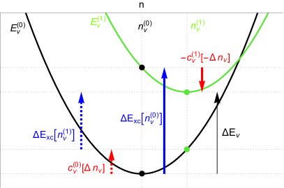
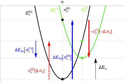
Figure 1: Cartoon showing the density-driven and functional-driven contributions to $\Delta E_{v}$ (Eqs. 19 and 20) in an energy-driven difference (top panel) and a density-driven difference (bottom panel)

By virtue of Eq. 17, the $\Delta E_{{}_{\scriptscriptstyle\rm XC}}[n_{v}^{(i)}]$ quantity represents the difference between the two functionals evaluated on each density. Therefore, we can identify $\Delta E_{{}_{\scriptscriptstyle\rm XC}}[n_{v}^{(1)}]$ and $\Delta E_{{}_{\scriptscriptstyle\rm XC}}[n_{v}^{(0)}]$ of Eqs. 19 and 20 as functional-driven terms. On the other hand, $D_{v}^{(0)}[n_{v}^{(1)}]$ and $D_{v}^{(1)}[n_{v}^{(0)}]$ are the density-driven terms, as they are given by the difference between the same energy functional evaluated on different densities. Generalizing the ideas of DC-DFT [13, 14, 21, 22, 23, 24, 25], for any pair of density functionals, we classify a $\Delta E_{v}$ energy difference as energy- or density-driven. We consider energy-driven $\Delta E_{v}$ as ones whose functional-driven terms in Eqs. 19 and 20 strongly dominate the density-driven terms (i.e.$\left|\Delta E_{{}_{\scriptscriptstyle\rm XC}}[n_{v}^{(0)}]\right|>>D_{v}^{(1)}[-\Delta n_{v}]$ and $\left|\Delta E_{{}_{\scriptscriptstyle\rm XC}}[n_{v}^{(1)}]\right|>>D_{v}^{(0)}[\Delta n_{v}]$). On the other hand, in density-driven cases the density-driven terms are no longer negligible. In Figure 1, we show the two density-driven and the two functional-driven contributions to their energy difference in a cartoon representing an energy-driven difference (top panel) and a density-driven difference (bottom panel). Measures that quantify density-driven character in a given system (again for a given pair of functionals) will be introduced and discussed in Section V.

III.   Density functional interpolation

To derive an exact expression for $\Delta E_{v}$ by smoothly connecting $E_{{}_{\scriptscriptstyle\rm XC}}^{(0)}[n]$ to $E_{{}_{\scriptscriptstyle\rm XC}}^{(1)}[n]$, we introduce the $\alpha$-parameter dependent XC functional:

$$E_{{}_{\scriptscriptstyle\rm XC}}^{(\alpha)}[n]=E_{{}_{\scriptscriptstyle\rm XC}}^{(0)}[n]+\alpha\Delta E_{{}_{\scriptscriptstyle\rm XC}}[n].$$ (22)

The corresponding total energy functional reads as:

$$E_{v}^{(\alpha)}[n]=\underbrace{F_{{}_{\scriptscriptstyle\rm SH}}[n]+n\cdot v+E_{{}_{\scriptscriptstyle\rm XC}}^{(0)}[n]}_{E_{v}^{(0)}[n]}+\alpha\Delta E_{{}_{\scriptscriptstyle\rm XC}}[n]$$ (23)

and achieves its minimum at $n_{v}^{(\alpha)}({\bf r})$. Thus its ground state energy is given by $E_{v}^{(\alpha)}=E_{v}^{(\alpha)}[n_{v}^{(\alpha)}]$. More generally, we consider the following energy difference:

$$\Delta E_{v}^{(\alpha)}=E_{v}^{(\alpha)}-E_{v}^{(0)}=E_{v}^{(\alpha)}[n_{v}^{(\alpha)}]-E_{v}^{0}[n_{v}^{(0)}].$$ (24)

Writing:

$$\Delta E_{v}^{(\alpha)}=\int_{0}^{\alpha}d\alpha^{\prime}\,\frac{\partial E_{v}^{(\alpha^{\prime})}}{\partial\alpha^{\prime}},$$ (25)

from Eq. 23, via the Hellmann-Feynman theorem, it follows:

$$\frac{\partial E_{v}^{(\alpha)}}{\partial\alpha}=\Delta E_{{}_{\scriptscriptstyle\rm XC}}[n_{v}^{(\alpha)}].$$ (26)

Plugging Eq. 26 into Eq. 25, we find:

$$\Delta E_{v}^{(\alpha)}=\int_{0}^{\alpha}d\alpha^{\prime}\,\Delta E_{{}_{\scriptscriptstyle\rm XC}}[n_{v}^{(\alpha^{\prime})}].$$ (27)

Equation 27 is analogous to, but different from, the adiabatic connection formula for the correlation energy in DFT [26, 27, 28]. When $\alpha=1$, Eq. 27 becomes:

$$\Delta E_{v}=\int_{0}^{1}d\alpha\,\Delta E_{{}_{\scriptscriptstyle\rm XC}}[n_{v}^{(\alpha)}].$$ (28)

This shows that the energy difference between two KS calculations with different XC functionals can be found knowing only the difference functional and the interpolating ground-state density. Obtaining $\Delta E_{v}$ from Eq. 28 requires knowledge of $n_{v}^{(\alpha)}({\bf r})$ for all $\alpha$ values between $0$ and $1$. To find $n_{v}^{(\alpha)}({\bf r})$, we write the corresponding Euler equation:

$$v_{{}_{\scriptscriptstyle\rm SHXC}}^{(0)}[n]({\bf r})+\alpha\Delta v_{{}_{\scriptscriptstyle\rm XC}}[n]({\bf r})+v({\bf r})=\mu.$$ (29)

where $v_{{}_{\scriptscriptstyle\rm SHXC}}^{(0)}[n]({\bf r})=\delta F^{(0)}[n]/\delta n({\bf r})$, and where $\mu$ is the chemical potential. The role of $\mu$ is not relevant here, as we always keep the number of electrons fixed. The density that satisfies Eq. 29 is $n_{v}^{(\alpha)}({\bf r})$, and by expanding it around $n_{v}^{(0)}({\bf r})$: $n_{v}^{(\alpha)}({\bf r})=n_{v}^{(0)}({\bf r})+\alpha\Delta n_{v}^{(\alpha)}({\bf r})$, we can write Eq. 29 as:

$$v_{{}_{\scriptscriptstyle\rm SHXC}}^{(0)}[n_{v}^{(0)}]({\bf r})+\alpha\left[K_{v}^{(0)}\cdot\Delta n_{v}^{(\alpha)}\right]({\bf r})$$

$$+\alpha\left(\Delta v_{{}_{\scriptscriptstyle\rm XC}}[n_{v}^{(0)}]({\bf r})+\alpha\left[\Delta f_{{}_{\scriptscriptstyle\rm XC}}\left[n_{v}^{(0)}\right]\cdot\Delta n_{v}^{(\alpha)}\right]({\bf r})\right)+v({\bf r})$$

$$=\mu,$$ (30)

where we simplified the notation for the following integral:

$$\left[A\cdot\Delta n\right]({\bf r})=\int d^{3}r^{\prime}\,A({\bf r},{\bf r}^{\prime})\Delta n({\bf r}^{\prime}).$$ (31)

At $\alpha=0$, Eq. 29 becomes:

$$v_{{}_{\scriptscriptstyle\rm SHXC}}^{(0)}[n_{v}^{(0)}]({\bf r})+v({\bf r})=\mu$$ (32)

Plugging Eq. 32 into Eq. III gives:

$$\left[K_{v}^{(0)}[n_{v}^{(0)}]\cdot\Delta n_{v}^{(\alpha)}\right]({\bf r})+\Delta v_{{}_{\scriptscriptstyle\rm XC}}[n_{v}^{(0)}]({\bf r})$$

$$+\alpha\left[\Delta f_{{}_{\scriptscriptstyle\rm XC}}[n_{v}^{(0)}]\cdot\Delta n_{v}^{(\alpha)}\right]({\bf r})=0.$$ (33)

Also plugging $K_{v}^{(\alpha)}({\bf r},{\bf r}^{\prime})=K_{v}^{(0)}({\bf r},{\bf r}^{\prime})+\alpha\Delta f_{{}_{\scriptscriptstyle\rm XC}}({\bf r},{\bf r}^{\prime})$ (Eqs. 11 and 23) into Eq III, we obtain:

$$\int d^{3}r^{\prime}\,K_{v}^{(\alpha)}[n_{v}^{(0)}]({\bf r},{\bf r}^{\prime})\,\Delta n_{v}^{(\alpha)}({\bf r}^{\prime})=-\Delta v_{{}_{\scriptscriptstyle\rm XC}}[n_{v}^{(0)}]({\bf r}).$$ (34)

In principle, $\Delta n_{v}^{\alpha}({\bf r}^{\prime})$ can be obtained by solving Eq. 34, and we can write the solution in terms of the inverse of $K_{v}^{(\alpha)}[n_{v}^{(0)}]$:

$$\Delta n_{v}^{(\alpha)}({\bf r})=-\int d^{3}r^{\prime}\,\left\{K_{v}^{(\alpha)}\right\}^{-1}\,[n_{v}^{(0)}]({\bf r},{\bf r}^{\prime})\,\Delta v_{{}_{\scriptscriptstyle\rm XC}}[n_{v}^{(0)}]({\bf r}^{\prime}).$$ (35)

We expect that $\Delta n_{v}^{(\alpha)}({\bf r})$ of Eq. 35 can be fairly approximated by $\Delta n_{v}$ and this is equivalent to approximating $n_{v}^{(\alpha)}$ via the following linear interpolation:

$$n_{v}^{(\alpha)}({\bf r})\approx n_{v}^{(0)}({\bf r})+\alpha\Delta n_{v}({\bf r}).$$ (36)

To explore in what situation the approximation of Eq. 36 becomes exact, we now write $n_{v}^{(\alpha)}$ as : $n_{v}^{(\alpha)}({\bf r})=n_{v}^{(1)}({\bf r})-\bar{\alpha}\Delta n_{v}^{(\alpha)^{\prime}}$, where $\bar{\alpha}=1-\alpha$. Repeating the steps given by Eqs. 29 to 35, we find:

$$\Delta n_{v}^{(\alpha)^{\prime}}({\bf r})=-\int d^{3}r^{\prime}\,\left\{K_{v}^{(\alpha)}\right\}^{-1}\,[n_{v}^{(1)}]({\bf r},{\bf r}^{\prime})\,\Delta v_{{}_{\scriptscriptstyle\rm XC}}[n_{v}^{(1)}]({\bf r}^{\prime}).$$ (37)

In this way, when $\Delta n_{v}^{(\alpha)^{\prime}}({\bf r})$ is equal to $\Delta n({\bf r})$ of Eq. 35, then the exact $n_{v}^{(\alpha)}$ is indeed given by the r.h.s of Eq. 36.

To obtain the leading order of $E_{v}^{(\alpha)}$ in powers of $\alpha$, we set again: $n_{v}^{\alpha}({\bf r})=n_{v}^{(0)}({\bf r})+\alpha\Delta n_{v}^{(\alpha)}({\bf r})$. Then, $E_{v}^{(\alpha)}$ becomes:

$$E_{v}^{(\alpha)}[n_{v}^{(\alpha)}]= F_{{}_{\scriptscriptstyle\rm SH}}[n_{v}^{(0)}+\alpha\Delta n_{v}^{(\alpha)}]+n_{v}^{(0)}\cdot v$$

$$+\alpha\Delta n_{v}^{(\alpha)}\cdot v+E_{{}_{\scriptscriptstyle\rm XC}}^{(0)}[n_{v}^{(0)}+\alpha\Delta n_{v}^{(\alpha)}]$$

$$+\alpha\Delta E_{{}_{\scriptscriptstyle\rm XC}}[n_{v}^{(0)}+\alpha\Delta n_{v}^{(\alpha)}].$$ (38)

We can expand $E_{v}^{(\alpha)}[n_{v}^{(0)}+\alpha\Delta n_{v}^{(\alpha)}]$ around $n_{v}^{(0)}({\bf r})$, and write $E_{v}^{(\alpha)}$ in powers of $\alpha$:

$$E_{v}^{(\alpha)}= E_{v}^{(0)}[n_{v}^{(0)}]+\alpha\Delta E_{{}_{\scriptscriptstyle\rm XC}}[n_{v}^{(0)}]$$

$$+\alpha\left(v_{{}_{\scriptscriptstyle\rm SHXC}}^{(0)}[n_{v}^{(0)}]+v\right)\cdot\Delta n_{v}^{(\alpha)}$$

$$+\alpha^{2}\left(\Delta v_{{}_{\scriptscriptstyle\rm XC}}[n_{v}^{(0)}]\cdot\Delta n_{v}^{(\alpha)}+\frac{1}{2}K_{v}^{(0)}\left[\Delta n_{v}^{(\alpha)}\right]\right)$$

$$+\mathcal{O}(\alpha^{3})$$ (39)

Combining Eqs. 32 and III, the third term on the r.h.s of Eq. III vanishes:

$$E_{v}^{(\alpha)}= E_{v}^{(0)}[n_{v}^{(0)}]+\alpha\Delta E_{{}_{\scriptscriptstyle\rm XC}}[n_{v}^{(0)}]$$

$$+\alpha^{2}\left(\frac{1}{2}K_{v}^{(0)}\left[\Delta n_{v}^{(\alpha)}\right]+\Delta v_{{}_{\scriptscriptstyle\rm XC}}[n_{v}^{(0)}]\cdot\Delta n_{v}^{(\alpha)}\right)$$

$$+\mathcal{O}(\alpha^{3}).$$ (40)

Using Eq. 34, we can further simplify Eq. III:

$$E_{v}^{(\alpha)}= E_{v}^{(0)}[n_{v}^{(0)}]+\alpha\Delta E_{{}_{\scriptscriptstyle\rm XC}}[n_{v}^{(0)}]+\frac{\alpha^{2}}{2}\Delta v_{{}_{\scriptscriptstyle\rm XC}}[n_{v}^{(0)}]\cdot\Delta n_{v}^{(\alpha)}$$

$$+\mathcal{O}(\alpha^{3}).$$ (41)

From Eq. III, we can see that to leading order in $\alpha$, the $\alpha$-dependence of the minimizing energies is quadratic, and it can be found from the xc energies and xc potentials at the endpoints. We can also use the following functional expansion:

$$\Delta E_{{}_{\scriptscriptstyle\rm XC}}\left[n_{v}^{(0)}+\frac{\alpha}{2}\Delta n_{v}^{(\alpha)}\right]=$$

$$\Delta E_{{}_{\scriptscriptstyle\rm XC}}\left[n_{v}^{(0)}\right]+\frac{\alpha}{2}\Delta v_{{}_{\scriptscriptstyle\rm XC}}\left[n_{v}^{(0)}\right]\cdot\Delta n_{v}^{(\alpha)}+\mathcal{O}(\alpha^{2}),$$ (42)

and plug it into Eq. III to finally obtain:

$$E_{v}^{(\alpha)}=E_{v}^{(0)}\left[n_{v}^{(0)}\right]+\alpha\Delta E_{{}_{\scriptscriptstyle\rm XC}}\left[n_{v}^{(0)}+\frac{\alpha}{2}\Delta n_{v}^{(\alpha)}\right]+\ldots$$ (43)

Similarly, writing $n_{v}^{(\alpha)}=n_{v}^{(1)}({\bf r})-\bar{\alpha}\Delta n_{v}^{(\alpha)}({\bf r})$, we can expand $E_{v}^{(\alpha)}$ around $n_{v}^{(1)}$ to obtain:

$$E_{v}^{(\alpha)}=E_{v}^{(1)}\left[n_{v}^{(1)}\right]-\bar{\alpha}\Delta E_{{}_{\scriptscriptstyle\rm XC}}\left[n_{v}^{(1)}-\frac{\bar{\alpha}}{2}\Delta n_{v}^{(\alpha)}\right]+\ldots$$ (44)

Both results are consistent with applying Eq. 27 and expanding only the density to first order in $\alpha$. In Section IVC, we will illustrate the usefulness of the formalism developed in this section for connecting a global hybrid functional to its parent GGA.

IV.   Specific cases

A.   Quantifying errors with DC-DFT

There has been recent great interest in quantifying the errors in densities in DFT [29, 30, 31, 32]. However, in Ref [25], it was shown that the theory of DC-DFT provides a natural and unambiguous measure of density error. With that measure, it was not possible to distinguish the densities of empirical and non-empirical functionals based on their self-consistent densities alone.

To understand the background to this, we first must distinguish ground-state KS DFT from other areas of electronic structure. The primary purpose of such calculations is to produce the ground-state energy as a function of nuclear coordinates. Indeed, in principle, one can deduce the density (and hence any integral over it) from a sequence of such calculations, via the functional derivative with respect to the potential. Of course, such calculations produce KS potentials, orbitals, and eigenvalues, as well as densities and ground-state energies, and all such quantities can be compared (for systems for which the calculation is feasible) to their exact counterparts extracted from a more accurate quantum solver [33, 34, 35]. These are of great interest as inputs to response calculations, such as in linear-response TDDFT or GW methods, and such procedures might be extremely sensitive to such inputs. But in ground-state DFT, the main prediction is the energy of the many-body system, for which the KS scheme is simply a brilliant construct that balances efficiency and accuracy.

Intuitively, one feels that a ’better’ XC potential must yield a ’better’ density, and in turn, a ’better’ density must yield a better energy. After all, the Hohenberg-Kohn (HK) theorem tells us that we reach the ground-state energy only with the exact density and exact KS potential. But such formal statements give no measure of the quality of a density or a potential. Even a well-defined mathematical norm between two densities that vanishes as the exact density is approached does not really provide what we wish for, as an infinity of arbitrarily different norms can be constructed. All can tell us when we have found the exact density, but give differing results for how far away we are from it. A deep part of the problem is that both potentials and densities are functions of ${\bf r}$, and so are not characterized by a single number.

As mentioned in Ref [25], the basic theorems of DFT give us an ideal solution to this dilemma, via density-corrected DFT. To write this measure in the language of the density functional analysis, we consider now the specific case where $E_{{}_{\scriptscriptstyle\rm XC}}^{(0)}[n]=E_{{}_{\scriptscriptstyle\rm XC}}[n]$ is the exact XC functional and where $E_{{}_{\scriptscriptstyle\rm XC}}^{(1)}[n]=\tilde{E}_{{}_{\scriptscriptstyle\rm XC}}[n]$ is an approximate functional. Note also that this is the basis of all DC-DFT applications. For a given $v({\bf r})$, the difference between the two corresponding ground state energies becomes the error in the approximate ground-state energy:

$$\Delta\tilde{E}_{v}=\tilde{E}_{v}-E_{v}.$$ (45)

For this special case, Eq. 20 becomes:

$$\Delta\tilde{E}_{v}=\underbrace{\tilde{E}_{v}[\tilde{n}_{v}]-E_{v}[\tilde{n}_{v}]}_{\Delta\tilde{E}_{{}_{\scriptscriptstyle\rm XC}}[\tilde{n}_{v}]}+\underbrace{E_{v}[\tilde{n}_{v}]-E_{v}[n_{v}]}_{\Delta E^{ideal}[\Delta\tilde{n}_{v}]=D_{v}[\Delta\tilde{n}_{v}]}.$$ (46)

where $\Delta\tilde{n}_{v}=\tilde{n}_{v}-n_{v}$. For any system, $\Delta E^{ideal}[\Delta\tilde{n}_{v}]$ is a positive energy for any $\tilde{n}_{v}({\bf r})$ and vanishes only for the exact density. This choice is ideal because (a) there are no human choices within the measure to argue over, and (b) the measurement is in terms of the energetic consequences. Thus it even provides a scale for density differences. For example, if this measure yields results in the microHartree range, why would one even care about errors in the density? Given that it is very difficult in practice to evaluate the exact functional on an approximate density (but see e.g., Refs. [36] and [37]), DC-DFT procedures use the following equation instead:

$$\Delta\tilde{E}_{v}=\underbrace{\tilde{E}_{v}[\tilde{n}_{v}]-\tilde{E}_{v}[n_{v}]}_{\Delta E_{{}_{\scriptscriptstyle\rm D}}=-\tilde{D}_{v}[-\Delta\tilde{n}_{v}]}+\underbrace{\Delta\tilde{E}_{{}_{\scriptscriptstyle\rm XC}}[n_{v}]}_{\Delta E_{{}_{\scriptscriptstyle\rm F}}}.$$ (47)

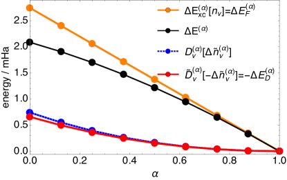
Figure 2: Various errors of Eqs. 52 and 53 for the $\alpha$-BLYP calculations of the hydrogen atom as a function of amount of exact exchange mixing

Equation 47 allows us to decompose $\Delta\tilde{E}_{v}$, the total error made by $\tilde{E}_{{}_{\scriptscriptstyle\rm XC}}[n]$ and $\tilde{n}_{v}$, into the functional error $\Delta E_{{}_{\scriptscriptstyle\rm F}}=\Delta\tilde{E}_{{}_{\scriptscriptstyle\rm XC}}[n_{v}]$ and the density-driven error $\Delta E_{{}_{\scriptscriptstyle\rm D}}=-\tilde{D}_{v}[-\Delta\tilde{n}_{v}]$, which is much more practical than the ideal, as it needs only be evaluated on the approximate functional. We can in fact expect $\Delta E_{{}_{\scriptscriptstyle\rm D}}$ to be a practical proxy for the intractable $E^{ideal}[\Delta\tilde{n}_{v}]$ measure. When the approximate density is sufficiently close to its exact counterpart (more precisely, when the two inequalities hold: $D_{v}[\Delta\tilde{n}_{v}]\leq\Delta_{c}$ and $\tilde{D}_{v}[-\Delta\tilde{n}_{v}]\leq\Delta_{c}$), we can write $\Delta E^{ideal}[\Delta\tilde{n}_{v}]$ as:

$$\Delta E^{ideal}[\Delta\tilde{n}_{v}]\approx\frac{1}{2}K_{v}[\Delta\tilde{n}_{v}],$$ (48)

and $\tilde{D}_{v}[-\Delta n_{v}]$ as:

$$\tilde{D}_{v}[-\Delta\tilde{n}_{v}]\approx\frac{1}{2}\tilde{K}_{v}[\Delta\tilde{n}_{v}]$$ (49)

From Eqs. 48 and 49, we can see that if the approximate functional has accurate curvature, $\tilde{D}_{v}[-\Delta\tilde{n}_{v}]=-\Delta E_{{}_{\scriptscriptstyle\rm D}}$ measure is very similar to $\Delta E^{ideal}[\Delta\tilde{n}_{v}]$.

B.   Illustration

Figure 2 illustrates many aspects of the analysis described so far. Here we consider the hydrogen atom and the BLYP GGA [38, 39]. We choose this example carefully, because (a) we have easy access to the exact density, since this is a one-electron case, and (b) our functional correctly has no correlation energy (as LYP correlation vanishes for all fully spin-polarized systems). Thus, when we interpolate between BLYP and HF, we create a global hybrid with a fraction $\alpha$ of exact exchange (EXX):

$$\tilde{E}_{{}_{\scriptscriptstyle\rm XC}}^{(\alpha)}[n]=\tilde{E}_{{}_{\scriptscriptstyle\rm XC}}^{{}^{\rm GGA}}[n]+\alpha\left(E_{{}_{\scriptscriptstyle\rm X}}[n]-\tilde{E}_{{}_{\scriptscriptstyle\rm X}}^{{}^{\rm GGA}}[n]\right).$$ (50)

For this specific cases $\tilde{E}_{{}_{\scriptscriptstyle\rm XC}}^{(\alpha)}[n]$ reduces to:

$$\tilde{E}_{{}_{\scriptscriptstyle\rm XC}}^{(\alpha)}[n]=\tilde{E}_{{}_{\scriptscriptstyle\rm X}}^{\rm B88}[n]+\alpha\left(E_{{}_{\scriptscriptstyle\rm X}}[n]-\tilde{E}_{{}_{\scriptscriptstyle\rm X}}^{\rm B88}[n]\right),$$ (51)

where $E_{{}_{\scriptscriptstyle\rm X}}^{\rm B88}[n]$ stands for the exchange functional of Becke [38]. For the $\Delta\tilde{E}_{v}^{(\alpha)}=\tilde{E}_{v}^{(\alpha)}-E_{v}$ energy difference (i.e. the error of the hybrids functional), we can rewrite Eq. 47 as:

$$\Delta\tilde{E}_{v}^{(\alpha)}=\underbrace{-\tilde{D}_{v}^{(\alpha)}[-\Delta\tilde{n}_{v}^{(\alpha)}]}_{\Delta E_{{}_{\scriptscriptstyle\rm D}}^{(\alpha)}} +\underbrace{\Delta\tilde{E}_{{}_{\scriptscriptstyle\rm XC}}^{(\alpha)}[n_{v}]}_{\Delta E_{{}_{\scriptscriptstyle\rm F}}^{(\alpha)}},$$ (52)

where $\Delta\tilde{n}_{v}^{(\alpha)}=\tilde{n}_{v}^{(\alpha)}-n_{v}$. In Eq. 52, we can recognize $\alpha$-dependent density-driven and functional errors. In the same manner, we can re-write Eq. 46:

$$\Delta\tilde{E}_{v}^{(\alpha)}=\Delta\tilde{E}_{{}_{\scriptscriptstyle\rm XC}}^{(\alpha)}[\tilde{n}_{v}^{(\alpha)}]+D_{v}[\Delta\tilde{n}_{v}^{(\alpha)}].$$ (53)

In this case, all error contributions (Eqs. 52 and 53), shown in Figure 2, vanish at $\alpha=1$. On the extreme left ($\alpha=0$), we see the functional error exceeds the self-consistent error, and the density-driven error is negative, as it should be. The functional error is exactly linear, going to zero as $\alpha\to 1$. Notice that the density-driven error must always behave parabolically around $\alpha=1$.

We also compare the two choices of reference for $D_{v}$ (blue and red), finding that they are almost identical. This is telling us that the BLYP density is sufficiently close to the exact density that the expansion to second-order is fine. Moreover, note that as $\alpha\to 1$, the blue and red merge datapoints, and both are on top of a perfect parabola whose curvature is given by $K_{v}[\Delta n]$ (again as $\alpha\to 1$). Since the self-consistent error is the sum of the functional and density-driven errors, we can deduce its curve just from the values at $\alpha=0$. Thus the black line is always a parabola if the densities are sufficiently similar, as is the case here. Note that we can see that the energetic difference between the $D_{v}$ values (blue and red plots) is rather low, showing that they are indeed sufficiently close that there are no significant energetic consequences to approximating all such curves as parabolas.

Finally, we note that, relative to DC-DFT, we have chosen the two functionals in the reverse order: 0 denotes the approximate functional, 1 the exact answer. This is to make these results more readily comparable to other results for hybrids. Simply replace $\alpha$ by $1-\alpha$ to make Fig. 2 in the form for DC-DFT.

C.   Self-interaction error and one-electron systems

For one-electron systems:

$$F[n]=T_{{}_{\scriptscriptstyle\rm S}}[n],\,E_{{}_{\scriptscriptstyle\rm X}}[n]=-U_{\scriptscriptstyle\rm H}[n],\,E_{{}_{\scriptscriptstyle\rm C}}=0\leavevmode\nobreak\ \leavevmode\nobreak\ \leavevmode\nobreak\ \leavevmode\nobreak\ \leavevmode\nobreak\ (N=1).$$ (54)

Standard DFT approximations typically do not satisfy all the conditions of Eq 54, and for this reason, they suffer from one-electron self-interaction error (SIE) [6, 40]. On the other hand, the HF method is exact for one-electron systems, and thus we can use the HF method to calculate the functional- and density-driven term of SIE.

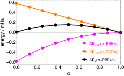
Figure 3: Density-driven and functional errors for the $\alpha$-PBExc (Eq. 55) calculations of the hydrogen atom as a function of amount of exact exchange mixing

This has been already done in Figure 2 for the BLYP hybrids, and in Figure 3 we apply the same analysis to hybrids from the PBE functional [41]. The PBE correlation energy, unlike that of LYP, does not vanish for one-electron systems. For this reason, in the case of the PBE functional we modify Eq. 50:

$$\tilde{E}_{{}_{\scriptscriptstyle\rm XC}}^{(\alpha)}[n]=\tilde{E}_{{}_{\scriptscriptstyle\rm XC}}^{{}^{\rm PBE}}[n]+\alpha\leavevmode\nobreak\ (E_{{}_{\scriptscriptstyle\rm X}}[n]-\tilde{E}_{{}_{\scriptscriptstyle\rm XC}}^{{}^{\rm PBE}}[n]),$$ (55)

In this way, we ensure that the error of the PBE hybrid of Eq. 55 (hereinafter $\alpha$-PBExc) vanishes at $\alpha=1$ Note that this does not include PBE0 [42], as this PBExc has only 0.75 of PBE correlation at $\alpha=1/4$. In Figure 3, we show the density-driven and functional error of $\alpha$-PBExc for the hydrogen atom. First, note that the scale of the errors is minuscule. We can also see that both $|\Delta E_{{}_{\scriptscriptstyle\rm F}}^{(\alpha)}|$ and $|\Delta E_{{}_{\scriptscriptstyle\rm D}}^{(\alpha)}|$ errors of $\alpha$-PBExc decrease with $\alpha$. Nonetheless, its total $\Delta E^{(\alpha)}$ error peaks at $\alpha\approx 0.5$ and nearly vanishes for the PBE functional (the $\alpha=0$ case). The fact that the PBE gives almost exact energy for the hydrogen atom relies on a cancellation between the functional and density-driven errors (as well as a cancellation between exchange and correlation errors).

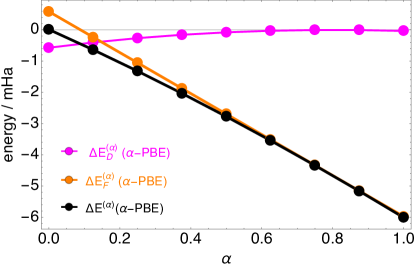
Figure 4: Density-driven and functional errors for the $\alpha$-PBE (Eq.50) calculations of the hydrogen atom as a function of amount of exact exchange mixing

The same plot for the hydrogen atom obtained with the regular $\alpha$-PBE hybrid (Eq. 50) is shown in Figure 4. Note that now the $\alpha=1/4$ point represents the PBE0 functional. We can see from Figure 4 that as $\alpha$ approaches $1$, the functional error strongly dominates its functional-driven counterpart. Note here the much larger scale: The self-interaction error in the PBE correlation functional error yields much larger total energy errors than in the previous figure, illustrating the increased error when semilocal correlation functionals are combined with exact exchange. We can also note that $E_{{}_{\scriptscriptstyle\rm D}}$ gets very close to $0$ as $\alpha$ approaches $1$, although the PBE correlation potential does not vanish for $N=1$ systems.

D.   The Hartree approximation

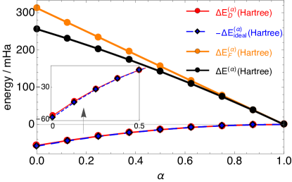
Figure 5: Density-driven, the ideal, and functional errors for the hydrogen atom calculation with the $\tilde{E}_{{}_{\scriptscriptstyle\rm XC}}^{(\alpha)}[n]=\alpha\tilde{E}_{{}_{\scriptscriptstyle\rm X}}^{(\alpha)}[n]$ functional.

Another special case is the Hartree approximation, i.e., solution of the KS equations with XC set to zero. Here, we compare any non-zero $\tilde{E}_{\scriptscriptstyle\rm XC}$ with pure Hartree. We choose Hartree to be $\alpha=0$, so that $\alpha$ then represents the fraction of $\tilde{E}_{\scriptscriptstyle\rm XC}$ included in the calculation. While Hartree calculations are certainly too inaccurate for chemical purposes [43, 44], one would expect them to have the greatest delocalization error of any approximate functional, since not even LDA exchange is opposing the Hartree energy. They might thus prove useful in creating a non-empirical measure of delocalization to be used in DC-DFT.

If the reference is the exact XC energy, then the functional difference is just the XC energy itself, while the density-driven error is just: $\Delta E_{{}_{\scriptscriptstyle\rm D}}=-\frac{1}{2}f_{{\rm SH}}[n_{v}^{(0)},\Delta n]$. In this case, one would expect $E_{{}_{\scriptscriptstyle\rm D}}$ to be different from the ideal, which includes the XC contributions. However, as we will show below the two quantities are nearly the same for the hydrogen atom.

To give an illustration, we consider the following functional: $\tilde{E}_{{}_{\scriptscriptstyle\rm XC}}^{(\alpha)}[n]=\alpha E_{{}_{\scriptscriptstyle\rm X}}[n]$, which for one-electron systems connects the Hartree approximation ($\alpha=0$) to the exact functional ($\alpha=1$). In Figure 5, we show the errors of this functional as a function of $\alpha$ for the hydrogen atom. As expected, the scale of errors is much larger than those shown in Figures 2-4. We find it interesting that the $-\Delta E^{ideal}$ datapoints in Figure 5 are hardly distinguishable from their $\Delta E_{{}_{\scriptscriptstyle\rm D}}$ counterparts. Thus, at $\lambda=0$ we have:

$$\underbrace{f_{\scriptscriptstyle\rm S}[n_{v},\Delta n]}_{-2\Delta E^{ideal}}\sim\underbrace{f_{{\rm SH}}[n_{v}^{(0)},\Delta n]}_{-2\Delta E_{{}_{\scriptscriptstyle\rm D}}}\leavevmode\nobreak\ \leavevmode\nobreak\ \leavevmode\nobreak\ \leavevmode\nobreak\ \rm{(H\leavevmode\nobreak\ atom)},$$ (56)

where $f_{\scriptscriptstyle\rm S}({\bf r},{\bf r}^{\prime})$ is the kinetic component of $f_{{\rm SH}}({\bf r},{\bf r}^{\prime})$ (see Eq. 12).

E.   Pure density functionals

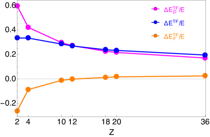
Figure 6: Plots showing quantities that involve the density-driven and functional errors of the Thomas-Fermi method (Eq. 58) with $Z$ for a range of small atoms.

So far, we have considered only approximations to XC within the KS scheme, as this is the most common DFT calculation today by far. However, there is much interest in developing orbital-free functionals, especially in contexts when the KS scheme becomes too cumbersome.

Since the entire functional $F[n]$ is approximated in such a scheme, the density is often much poorer than in a KS calculation. In fact, estimates suggest that simple orbital-free approximations, such as those used in Thomas-Fermi theory [45, 46, 47], produce sufficiently poor densities that their errors are dominated by errors in the density, i.e., the density-driven error is much larger than the functional error in most calculations. This is seen in total energy calculations of atoms and of one-dimensional fermions in a flat box [23]. The simplest DC-DFT in orbital-free DFT is to apply the approximation on the exact density to eliminate the density-driven error.

To exemplify the error analysis of orbital-free functionals, we consider here the TF energy functional, whose universal part reads as:

$$F^{{}^{\rm TF}}[n]=\underbrace{T_{{}_{\scriptscriptstyle\rm S}}^{{}^{\rm TF}}[n]}_{A^{{}^{\rm TF}}\int d^{3}r\,n({\bf r})^{5/3}}+U[n],$$ (57)

with $A^{{}^{\rm TF}}=\frac{3}{10}\left(3\pi^{2}\right)^{\frac{2}{3}}$. The total TF error can be, analogously to eq 47, partitioned as:

$$\Delta E_{v}^{{}^{\rm TF}}=\underbrace{E_{v}^{{}^{\rm TF}}[n_{v}^{{}^{\rm TF}}]-E_{v}^{{}^{\rm TF}}[n_{v}]}_{\Delta E_{{}_{\scriptscriptstyle\rm D}}^{\rm TF}}+\underbrace{\Delta F^{\rm TF}[n_{v}]}_{\Delta E_{{}_{\scriptscriptstyle\rm F}}^{\rm TF}},$$ (58)

where $\Delta F^{\rm TF}[n]=\Delta E_{v}^{\rm TF}[n]=\Delta T_{{}_{\scriptscriptstyle\rm S}}^{{}^{\rm TF}}[n]-E_{{}_{\scriptscriptstyle\rm XC}}[n]$. Here we calculate $\Delta E_{{}_{\scriptscriptstyle\rm D}}^{\rm TF}$ and $\Delta E_{{}_{\scriptscriptstyle\rm F}}^{\rm TF}$ for alkaline earth metals and noble gases up to krypton (Z=36). They are computed by utilizing that for neutral atoms: $E_{Z}^{\rm TF}\sim-0.7687\,Z^{7/3}$ [48]. Highly accurate energies and densities, i.e., $E_{v}$ and $n_{v}$ entering Eq. 58 have been obtained from the PySCF software [49] at the CCSD level within the aug-cc-pV$m$Z basis set [50], with the largest $m$ available for each of the atoms. From the plots shown in Figure 6, we can see that the density-driven component strongly dominates the total $\Delta E^{\rm TF}$ error. For example, in the case of the neon atom ($Z=10$) most of the TF error is practically density-driven, with $E_{{}_{\scriptscriptstyle\rm D}}^{\rm TF}/E\sim 28.4\%$ and $E_{{}_{\scriptscriptstyle\rm F}}^{\rm TF}/E$ being only $-1.3\%$! We remember that for neutral atoms, as $Z\to\infty$, the TF theory becomes relatively exact, in the sense that it satisfies: [51, 52, 53]

$$\lim_{Z\to\infty}\frac{\Delta E_{Z}^{\rm TF}}{E_{Z}}\to 0.$$ (59)

Thus, as $Z\to\infty$, our blue curve in Figure 6 should vanish. Nevertheless, in Figure 6 we are still far from this limit, as at our largest $Z$ value ($Z=36$), $\Delta E_{Z}^{\rm TF}/E_{Z}$ is around $1/5$.

This suggests several important points regarding these functionals. First, they must always be tested self-consistently, as tests of new orbital-free approximations on KS densities does not tell us much about their overall accuracy, given that the density-driven errors can be very large. At the same time, comparison of the functional on the KS density then provides enough information to separate functional- from density-driven errors, and we expect that even the KS densities obtained from the (semi)local XC approximations are sufficiently accurate for this purpose. Second, reports of failures of TF theory and its extensions should be revisited to determine if these are density-driven or functional-driven. If the former, one should focus on improving the densities rather than the total energies alone. Third, this supports efforts [54] to approximate the Pauli potential [55, 56] directly as a density functional, without requiring that the KS potential be a functional derivative.

In the context of the present paper, it should prove useful when comparing two orbital-free approximations to decompose their differences into functional- and density-driven contributions. If two different approximations differ in both contributions, this would suggest that good aspects of both might be combined to separately minimize each error.

F.   Strong correlation

In our last example, we show that density-driven errors can become large when systems are strongly correlated, but need not be. Generating a simple example is not so easy, as one needs essentially exact densities upon which to make evaluations and comparisons. Fortunately, the two-site two-fermion Hubbard model is an example where all quantities can be determined analytically. Many relevant KS-DFT quantities have been calculated exactly and summarized in two recent reviews, one on the ground-state[57] and one on linear-response TDDFT.[58]

For any two-electron system (in the absence of magnetic fields), the restricted HF functional is:

$$F^{RHF}[n]=T_{\scriptscriptstyle\rm S}[n]+U_{\scriptscriptstyle\rm H}[n]/2,$$ (60)

as half the Hartree is canceled by exchange, and correlation is ignored. In fact, the traditional definition of correlation energy in quantum chemistry, is

$$E_{\scriptscriptstyle\rm C}^{QC}=E-E^{RHF}[n^{RHF}].$$ (61)

Thus the energy-driven error of RHF is:

$$\Delta E_{F}=-E_{\scriptscriptstyle\rm C},$$ (62)

while the density-driven error is

$$\Delta E_{D}=E_{\scriptscriptstyle\rm C}-E_{\scriptscriptstyle\rm C}^{QC}.$$ (63)

For our 2-site model, the functional reduces to a simple function. The onsite occupations are $n_{1}$ and $n_{2}$, i.e., the density is just two non-negative real numbers. Moreover, since they always sum to 2, the density is fully represented by their difference. Likewise, we can choose the average potential to be zero and represent the inhomogeneity in the potential by a single number, $\Delta v$, the on-site potential difference. If we choose the hopping parameter $t=1/2$, the only other parameter is $U$, the energy cost of double occupation of a site.

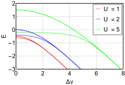
Figure 7: Restricted Hartree-Fock Hubbard dimer ground-state energy (dashed line) and exact Hubbard dimer ground-state (solid line) as functions of $\Delta v$ for varying values of $U$ (see Ref.[57]

The error in RHF and the exact ground state energy is explored in Figure 7 for varying levels of correlation and inhomogeneity. The absolute error increases with $U$, as expected. The energy error in energy for each level of correlation is most prominent in the symmetric dimer $(\Delta v=0)$, and diminishes and rapidly vanishes beyond $\Delta v$ larger than $U$, where the energy becomes linearly correlated with the on-site potential difference. Thus the system becomes weakly correlated for $\Delta v>U$.

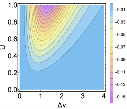
Figure 8: Fraction of error that is density-driven for moderate values of $U$, with the 5% contribution contour marked by a red, dashed line.

The functional-driven and density-driven contributions to this HF error were then isolated through the use of Eqs. 61, 62 and 63. The fraction of the total error attributed to the density-driven component $(\Delta E_{D}/E_{C}^{QC})$ is shown in Figure 8 for weakly correlated dimers with values of $U$ up to 1. As $U$ decreases in size, both the magnitude of total error and its density-driven contribution decrease substantially. For $U<0.5$, there is no $\Delta v$ for which there is a density-driven contribution greater than 5% of the total error. Of course, as $U\to 0$, this ratio must vanish, so this is not unexpected. But we also see that the density-driven error vanishes at $\Delta v=0$ for any value of $U$, no matter how large, for symmetry reasons. Thus even a strongly correlated system might have no density-driven error. Moreover, for $\Delta v>1+2U$, again the error is less than 5%, due to correlation being weakened by inhomogeneity. So for any given $U$, there is a maximum in the fraction of density-driven error as a function of $\Delta v$, and it is at non-zero $\Delta v$.

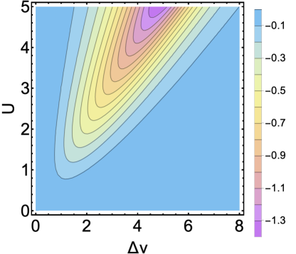
Figure 9: Same as Fig. 8, but zoomed out in $U$ and $\Delta v$. Note the change in contour/color scale.

The density-driven error ratio for more strongly correlated dimers is shown in Figure 9, and has characteristics identical to the weak correlation plot, but on a larger scale. Clearly the maximum fractional density-driven error becomes much larger with $U$ and can even exceed -$1$. We also see that for $U>1$, the region of small density-driven error around $\Delta v=0$ can even increase with $U$. For fixed $\Delta v$, the fraction of density-driven error goes down with sufficiently large $U$!. The relation between RHF density-driven error and strong correlation is clearly not trivial.

To avoid confusion, we note that this section has focused on the density-driven error in RHF. In the more realistic calculations of weakly-correlated systems in the rest of this work, we often assume that error is much smaller than the density-driven error of a semilocal DFT calculation, and hence HF-DFT yields more accurate energies in such cases. Because the Hubbard dimer is a site model, there is no genuine correspondence with semilocal DFT approximations to test on here.

V.   Energy differences

Key chemical concepts are determined by energy differences (e.g., atomization energies, ionization energies, barrier heights, reaction energies, etc.). For this reason, we extend our analysis to energy differences. For simplicity, we first look at the energy difference of systems A and B, whose external potentials are $v_{A}$ and $v_{B}$, respectively. This energy difference obtained from a total energy functional that corresponds to a given $E_{{}_{\scriptscriptstyle\rm XC}}^{(j)}$ is given by:

$$E_{AB}^{(j)}=E_{A}^{(j)}[n_{A}^{(j)}]-E_{B}^{(j)}[n_{B}^{(j)}].$$ (64)

When two functionals are involved, we can also define the difference between $E_{AB}^{(1)}$ and $E_{AB}^{(0)}$:

$$\Delta E_{AB}=E_{AB}^{(1)}-E_{AB}^{(0)}.$$ (65)

Plugging Eq. 64 into Eq. 65 gives:

$$\Delta E_{AB}=E_{A}^{(1)}[n_{A}^{(1)}]-E_{A}^{(0)}[n_{A}^{(0)}]-\Big{(}E_{B}^{(1)}[n_{B}^{(1)}]-E_{B}^{(0)}[n_{B}^{(0)}]\Big{)}.$$ (66)

Plugging Eq. 19 into Eq. 66, we can obtain the counterpart of Eq. 19 for the energy differences between systems A and B:

$$\Delta E_{AB}= \Delta E_{{}_{\scriptscriptstyle\rm XC}}[n_{A}^{(0)}]-E_{{}_{\scriptscriptstyle\rm XC}}[n_{B}^{(0)}]$$

$$\underbrace{-D_{A}^{(1)}[-\Delta n_{A}]+D_{B}^{(1)}[-\Delta n_{B}]}_{-D^{(1)}_{AB}}.$$ (67)

Similarly, we can also plug Eq. 20 into Eq. 66, to obtain the counterpart of Eq. 20 for the energy differences between systems A and B:

$$\Delta E_{AB}= \Delta E_{{}_{\scriptscriptstyle\rm XC}}[n_{A}^{(0)}]-\Delta E_{{}_{\scriptscriptstyle\rm XC}}[n_{B}^{(0)}]$$

$$+\underbrace{D_{A}^{(0)}[\Delta n_{A}]-D_{B}^{(0)}[\Delta n_{B}]}_{D^{(0)}_{AB}}.$$ (68)

In Eqs. V and V, we recognize $D^{(1)}_{AB}$ and $D^{(0)}_{AB}$ as the density-driven terms, pertinent to the energy differences between systems A and B. While $D_{v}^{(j)}$ of Eq. 6, which corresponds to the total energies is always greater or equal to $0$, its counterpart that pertains to the energy differences (Eqs. V and V) does not have a definite sign. Furthermore, if we look at $D^{(0)}_{AB}=D_{A}^{(0)}[\Delta n_{A}]-D_{B}^{(0)}[\Delta n_{B}]$ (Eq. V), where $D_{A}^{(0)}[\Delta n_{A}]\geq 0$ and $D_{B}^{(0)}[\Delta n_{B}]\geq 0$ we can see that $D^{(0)}_{AB}$ can easily vanish when $D_{A}^{(0)}[n_{A}^{(1)}]\sim D_{B}^{(0)}[n_{B}^{(1)}]$. Therefore, $D^{(0)}_{AB}$ and $D^{(1)}_{AB}$ can vanish even when $n_{A}^{(1)}$ and $n_{B}^{(1)}$ are drastically different from $n_{A}^{(0)}$ and $n_{B}^{(0)}$, respectively.

The shown example that involves the energy difference between systems A and B, can be easily generalized to any energy difference of interest. For instance, consider the following chemical reaction:

$$\sum_{l=1}^{L}{R}_{l}\to\sum_{m=1}^{M}{P}_{m},$$ (69)

where $\{R_{l}\}$ is a set of reactants and $\{P_{m}\}$ is a set of products. Then the energy of this reaction obtained from the $E_{v}^{(j)}[n]$ functional is:

$$E_{\rm ED}^{(j)}=\sum_{m=1}^{M}E_{P,m}^{(j)}[n_{P,m}^{(j)}]-\sum_{l=1}^{L}E_{R,l}^{(j)}[n_{R,l}^{(j)}].$$ (70)

The corresponding difference in $E_{\rm ED}^{(j)}$ between $j=0$ and $j=1$ functional is :

$$\Delta E_{\rm ED}=E_{\rm ED}^{(1)}-E_{\rm ED}^{(0)}.$$ (71)

Then $D_{\rm ED}^{(0)}$ that corresponds to $\Delta E_{\rm ED}$ is given by:

$$D_{\rm ED}^{(0)}=\sum_{m=1}^{M}D_{P,m}^{(0)}[\Delta n_{P,m}]-\sum_{l=1}^{L}D_{R,l}^{(0)}[\Delta n_{R,l}],$$ (72)

and its $D_{\rm ED}^{(1)}$ counterpart is given by:

$$D_{\rm ED}^{(1)}=\sum_{m=1}^{M}D_{P,m}^{(1)}[-\Delta n_{P,m}]-\sum_{l=1}^{L}D_{R,l}^{(1)}[-\Delta n_{R,l}].$$ (73)

Now that we established the density-driven terms of any energy difference of interest, we ask the following key question: how can we quantify the abnormality character of a given property/system obtained from a pair of functionals? Along these lines, we first define:

$$\Delta_{n}=\max{(|D^{(0)}|,|D^{(1)}|)}.$$ (74)

One would naturally think of the following indicator of abnormality:

$$\eta=\frac{\Delta_{n}}{\left|\Delta E_{\rm ED}\right|}.$$ (75)

Following this indicator, the abnormality character of a given property of interest increases with $\eta$. However, the $\eta$ indicator would be problematic when $\left|\Delta E_{\rm ED}\right|$ is small, and such properties/system will always be abnormal by default. To fix this problem, we introduce the abnormality scale. For a chosen property of interest (e.g., a barrier height involving organic molecules) we calculate the abnormality scale by using a dataset with similar systems/properties (e.g., other similar barrier heights involving organic molecules). We then set the abnormality as the root-mean-square of $K$ datapoints (i.e. $\Delta E_{\rm ED}$ energies) that form the dataset:

$$\bar{\Delta}_{\rm ED}=\sqrt{\frac{1}{K}\sum_{k=1}^{K}\left({\Delta E_{{\rm ED},k}}\right)^{2}},$$ (76)

Therefore, $\bar{\Delta_{\rm ED}}$ determines our abnormality scale, and it is specific to a given class of properties/system and to a given pair of energy functionals. Finally, we use $\Delta$ to define our abnormality indicator:

$$\bar{\eta}=\frac{\Delta_{n}}{\bar{\Delta}_{\rm ED}}$$ (77)

Also in the case of this indicator, the abnormality increases with $\bar{\eta}$. To classify systems as normal or abnormal (again for a given pair of functionals) based on the $\bar{\eta}$ indicator, we introduce a cut-off, e.g., $\bar{\eta}_{c}\sim\frac{1}{3}$, and consider abnormal systems/properties those that have $\bar{\eta}$ greater than $\bar{\eta}_{c}$. The primary goal of the present work is to outline the theory behind the density functional analysis. Therefore, showing numerical examples where we will illustrate (ab)-normality of different properties for different pairs of DFT approximations, we leave for future work.

Returning to DC-DFT, where functional 1 is some approximation and 0 is exact, we do not of course have access to $D^{(0)}$ in order to calculate $\bar{\eta}$, so we settle for $|D^{(1)}|$ alone, which is simply the usual density-driven error. But as noted in Ref. [25], that error would usually require knowing the exact density, which is usually either unavailable or unaffordable. (In normal systems, the HF density is NOT more accurate than the self-consistent density, and so cannot be used). A generic, practical workaround for standard approximations for use in HF-DFT is to define the density sensitivity of a functional as [25]:

$$\tilde{E}_{\scriptscriptstyle\rm DS}=\left|\tilde{E}[n_{\scriptscriptstyle\rm LDA}]-\tilde{E}[n_{\scriptscriptstyle\rm HF}]\right|,$$ (78)

which should always estimate $|D^{(1)}|$ when $|D^{(1)}|$ is a significant fraction of $\Delta$. Thus the PBE sensitivity is plotted in Fig 4 of Ref. [14], and averaged sensitivities were used in Table I of Ref. [25].

VI.   Conclusions

We have given a detailed account of the considerations that led to the recent successes of density-corrected DFT. We have also generalized that theory to allow different approximate functionals to be compared in the same way as DC-DFT allows one approximation to be compared with exact results. We have shown that typical density differences between reasonably accurate functionals can be shown quantitatively to be close enough to allow treatment via density functional analysis expansions truncated at second order. We consider different special cases of our analysis, and note that DC-DFT is just one of these. For a given pair of density functional approximations, we also construct measures for their relative abnormality (i.e. the situation when the density-driven terms strongly dominate the energy difference obtained with two different approximations).

We have noted many pioneering efforts in the chemistry literature in which density-corrected calculations were performed, usually based on intuition. We also point out that, as long ago as 1996, Levy and Görling advocated the use of self-consistent exact-exchange calculations, with a correction defined to produce the exact ground-state energy as a functional of the ‘wrong’ EXX density [59]. For purposes of calculating energies, the approach of Levy and Görling is nearly equivalent to HF-DFT, given that the EXX and HF densities are probably indistinguishable. Of course, we only advocate this procedure for abnormal systems, as in normal systems we expect the density from the standard semilocal approximations to be more accurate than that of HF.

Finally, we note that of course it is highly unsettling to run KS calculations in this non-self-consistent fashion. Many advantages that are often taken for granted, such as the exactness of the Hellmann-Feynman theorem in the basis-set limit, are no longer true, and many corrections need to be coded. But, in fact, all information about the density can be extracted from a sequence of total energy calculations, since:

$$n({\bf r})=\frac{\delta E_{v}}{\delta v({\bf r})}.$$ (79)

Treating HF as EXX, this leads to a predicted change in the density of a HF-DFT calculation relative to a self-consistent DFT density:

$$\Delta n({\bf r})=\frac{\delta(E^{DFT}[n^{\rm HF}]-E^{DFT}[n^{DFT}])}{\delta v({\bf r})}.$$ (80)

Thus, in principle, one could calculate the improvement to the density predicted by HF-DFT, and any other properties depending only on the density.

Acknowledgement

KB and JK acknowledge funding from NSF (CHE 1856165). SV acknowledges funding from the Rubicon project (019.181EN.026), which is financed by the Netherlands Organisation for Scientific Research (NWO). SS and ES were supported by the grant from the Korean Research Foundation (2017R1A2B2003552).

References

- [1] W. Kohn and L. J. Sham. Self-consistent equations including exchange and correlation effects. Phys. Rev., 140:A1133, 1965.
- [2] Aurora Pribram-Jones, David A Gross, and Kieron Burke. Dft: A theory full of holes? Annual review of physical chemistry, 66:283–304, 2015.
- [3] Stefan Grimme, Jens Antony, Stephan Ehrlich, and Helge Krieg. A consistent and accurate ab initio parametrization of density functional dispersion correction (dft-d) for the 94 elements h-pu. The Journal of chemical physics, 132(15):154104, 2010.
- [4] A. Savin. On degeneracy, near degeneracy and density functional theory. In J. M. Seminario, editor, Recent Developments of Modern Density Functional Theory, pages 327–357. Elsevier, Amsterdam, 1996.
- [5] A. J. Cohen, P. Mori-Sanchez, and W. Yang. Insights into current limitations of density functional theory. Science, 321:792, 2008.
- [6] Aron J. Cohen, Paula Mori-Sánchez, and Weitao Yang. Challenges for density functional theory. Chem. Rev., 112:289, 2012.
- [7] Roy G Gordon and Yung Sik Kim. Theory for the forces between closed-shell atoms and molecules. The Journal of Chemical Physics, 56(6):3122–3133, 1972.
- [8] Gustavo E. Scuseria. Comparison of coupled-cluster results with a hybrid of hartree–fock and density functional theory. J. Chem. Phys., 97(10):7528–7530, 1992.
- [9] Benjamin G Janesko and Gustavo E Scuseria. Hartree–fock orbitals significantly improve the reaction barrier heights predicted by semilocal density functionals. The Journal of chemical physics, 128(24):244112, 2008.
- [10] Peter MW Gill, Benny G Johnson, John A Pople, and Michael J Frisch. The performance of the becke—lee—yang—parr (b—lyp) density functional theory with various basis sets. Chemical Physics Letters, 197(4-5):499–505, 1992.
- [11] John C Slater. A simplification of the hartree-fock method. Phys. Rev., 81(3):385, 1951.
- [12] OV Gritsenko, ŁM Mentel, and EJ Baerends. On the errors of local density (lda) and generalized gradient (gga) approximations to the kohn-sham potential and orbital energies. J. Chem. Phys., 144(20):204114, 2016.
- [13] Min-Cheol Kim, Eunji Sim, and Kieron Burke. Understanding and reducing errors in density functional calculations. Phys. Rev. Lett., 111:073003, Aug 2013.
- [14] Yeil Kim, Suhwan Song, Eunji Sim, and Kieron Burke. Halogen and chalcogen binding dominated by density-driven errors. The journal of physical chemistry letters, 10(2):295–301, 2018.
- [15] Stefan Vuckovic, Tom J. P. Irons, Lucas O. Wagner, Andrew M. Teale, and Paola Gori-Giorgi. Interpolated energy densities, correlation indicators and lower bounds from approximations to the strong coupling limit of dft. Phys. Chem. Chem. Phys., 19:6169–6183, 2017.
- [16] Eduardo Fabiano, Paola Gori-Giorgi, Michael Seidl, and Fabio Della Sala. Interaction-strength interpolation method for main-group chemistry: Benchmarking, limitations, and perspectives. J. Chem. Theory Comput, 12(10):4885–4896, 2016.
- [17] Stefan Vuckovic, Paola Gori-Giorgi, Fabio Della Sala, and Eduardo Fabiano. Restoring size consistency of approximate functionals constructed from the adiabatic connection. J. Phys. Chem. Lett., 2018.
- [18] Kieron Burke. Perspective on density functional theory. J. Chem. Phys., 136(15):150901, 2012.
- [19] A. D. Becke. Perspective: Fifty years of density-functional theory in chemical physics. J. Chem. Phys., 140:18A301, 2014.
- [20] Matthias Ernzerhof. Taylor-series expansion of density functionals. Physical Review A, 50(6):4593, 1994.
- [21] Min-Cheol Kim, Eunji Sim, and Kieron Burke. Ions in solution: Density corrected density functional theory (dc-dft). J. Chem. Phys., 140(18):18A528, 2014.
- [22] Min-Cheol Kim, Hansol Park, Suyeon Son, Eunji Sim, and Kieron Burke. Improved dft potential energy surfaces via improved densities. J. Phys. Chem. Lett., 6(19):3802–3807, 2015.
- [23] Adam Wasserman, Jonathan Nafziger, Kaili Jiang, Min-Cheol Kim, Eunji Sim, and Kieron Burke. The importance of being inconsistent. Annual Review of Physical Chemistry, 68(1):555–581, 2017.
- [24] Suhwan Song, Min-Cheol Kim, Eunji Sim, Anouar Benali, Olle Heinonen, and Kieron Burke. Benchmarks and reliable dft results for spin gaps of small ligand fe(ii) complexes. Journal of Chemical Theory and Computation, 14(5):2304–2311, 2018.
- [25] Eunji Sim, Suhwan Song, and Kieron Burke. Quantifying density errors in dft. The journal of physical chemistry letters, 9(22):6385–6392, 2018.
- [26] J. Harris and R. Jones. The surface energy of a bounded electron gas. J. Phys. F, 4:1170, 1974.
- [27] David C Langreth and John P Perdew. The exchange-correlation energy of a metallic surface. Solid State Communications, 17(11):1425–1429, 1975.
- [28] O. Gunnarsson and B. I. Lundqvist. Exchange and correlation in atoms, molecules, and solids by the spin-density-functional formalism. Phys. Rev. B, 13:4274, 1976.
- [29] Michael G Medvedev, Ivan S Bushmarinov, Jianwei Sun, John P Perdew, and Konstantin A Lyssenko. Density functional theory is straying from the path toward the exact functional. Science, 355(6320):49–52, 2017.
- [30] Kasper P. Kepp. Comment on “density functional theory is straying from the path toward the exact functional”. Science, 356(6337):496–496, 2017.
- [31] Sharon Hammes-Schiffer. A conundrum for density functional theory. Science, 355(6320):28–29, 2017.
- [32] Martin Korth. Density functional theory: Not quite the right answer for the right reason yet. Angewandte Chemie International Edition, 56(20):5396–5398, 2017.
- [33] C. J. Umrigar and Xavier Gonze. Accurate exchange-correlation potentials and total-energy components for the helium isoelectronic series. Phys. Rev. A, 50:3827–3837, Nov 1994.
- [34] Qingsheng Zhao, Robert C. Morrison, and Robert G. Parr. From electron densities to kohn-sham kinetic energies, orbital energies, exchange-correlation potentials, and exchange-correlation energies. Phys. Rev. A, 50:2138–2142, Sep 1994.
- [35] Ilya G. Ryabinkin, Sviataslau V. Kohut, and Viktor N. Staroverov. Reduction of electronic wave functions to kohn-sham effective potentials. Phys. Rev. Lett., 115:083001, Aug 2015.
- [36] Lucas O Wagner, EM Stoudenmire, Kieron Burke, and Steven R White. Guaranteed convergence of the kohn-sham equations. Physical review letters, 111(9):093003, 2013.
- [37] Stefan Vuckovic, Tom JP Irons, Andreas Savin, Andrew M Teale, and Paola Gori-Giorgi. Exchange–correlation functionals via local interpolation along the adiabatic connection. J. Chem. Theory Comput., 12(6):2598–2610, 2016.
- [38] Axel D Becke. Density-functional exchange-energy approximation with correct asymptotic behavior. Phys. Rev. A, 38(6):3098, 1988.
- [39] Chengteh Lee, Weitao Yang, and Robert G Parr. Development of the colle-salvetti correlation-energy formula into a functional of the electron density. Physical review B, 37(2):785, 1988.
- [40] John P Perdew and Alex Zunger. Self-interaction correction to density-functional approximations for many-electron systems. Physical Review B, 23(10):5048, 1981.
- [41] J. P. Perdew, K. Burke, and M. Ernzerhof. Generalized gradient approximation made simple. Phys. Rev. Lett., 77:3865, 1996.
- [42] John P Perdew, Matthias Ernzerhof, and Kieron Burke. Rationale for mixing exact exchange with density functional approximations. J. Chem. Phys., 105(22):9982–9985, 1996.
- [43] John P Perdew and Karla Schmidt. Jacob’s ladder of density functional approximations for the exchange-correlation energy. In AIP Conference Proceedings, volume 577, pages 1–20. AIP, 2001.
- [44] John P Perdew. Climbing the ladder of density functional approximations. MRS bulletin, 38(9):743–750, 2013.
- [45] Llewellyn H Thomas. The calculation of atomic fields. In Mathematical Proceedings of the Cambridge Philosophical Society, volume 23, pages 542–548. Cambridge Univ Press, 1927.
- [46] Enrico Fermi. A statistical method for the determination of some priorieta dell’atome. Rend. Accad. Nat. Lincei, 6(602-607):32, 1927.
- [47] Elliott H Lieb and Barry Simon. The thomas-fermi theory of atoms, molecules and solids. Advances in mathematics, 23(1):22–116, 1977.
- [48] R. G. Parr and W. Yang. Density-Functional Theory of Atoms and Molecules. Oxford University Press, New York, 1989.
- [49] Qiming Sun, Timothy C Berkelbach, Nick S Blunt, George H Booth, Sheng Guo, Zhendong Li, Junzi Liu, James D McClain, Elvira R Sayfutyarova, Sandeep Sharma, et al. Pyscf: the python-based simulations of chemistry framework. Wiley Interdisciplinary Reviews: Computational Molecular Science, 8(1):e1340, 2018.
- [50] Thom H. Dunning. Gaussian basis sets for use in correlated molecular calculations. i. the atoms boron through neon and hydrogen. J. Chem. Phys., 90:1007, 1989.
- [51] Elliott H Lieb and Barry Simon. Thomas-fermi theory revisited. Physical Review Letters, 31(11):681, 1973.
- [52] Kieron Burke, Antonio Cancio, Tim Gould, and Stefano Pittalis. Locality of correlation in density functional theory. The Journal of chemical physics, 145(5):054112, 2016.
- [53] Antonio Cancio, Guo P Chen, Brandon T Krull, and Kieron Burke. Fitting a round peg into a round hole: Asymptotically correcting the generalized gradient approximation for correlation. The Journal of chemical physics, 149(8):084116, 2018.
- [54] Kati Finzel. Local conditions for the pauli potential in order to yield self-consistent electron densities exhibiting proper atomic shell structure. The Journal of chemical physics, 144(3):034108, 2016.
- [55] NH March. The local potential determining the square root of the ground-state electron density of atoms and molecules from the schrödinger equation. Physics Letters A, 113(9):476–478, 1986.
- [56] Mel Levy and Hui Ou-Yang. Exact properties of the pauli potential for the square root of the electron density and the kinetic energy functional. Physical Review A, 38(2):625, 1988.
- [57] D J Carrascal, J Ferrer, J C Smith, and K Burke. The hubbard dimer: a density functional case study of a many-body problem. Journal of Physics: Condensed Matter, 27(39):393001, 2015.
- [58] Diego J. Carrascal, Jaime Ferrer, Neepa Maitra, and Kieron Burke. Linear response time-dependent density functional theory of the hubbard dimer. The European Physical Journal B, 91(7):142, 07 2018.
- [59] Mel Levy and Andreas Görling. Correlation-energy density-functional formulas from correlating first-order density matrices. Phys. Rev. A, 52(3):R1808, 1995.