Higher Rank Numerical Ranges of Jordan-Like Matrices

Abstract.

We completely characterize the higher rank numerical range of the matrices of the form $J_{n}(\alpha)\oplus\beta I_{m}$, where $J_{n}(\alpha)$ is the $n\times n$ Jordan block with eigenvalue $\alpha$. Our characterization allows us to obtain concrete examples of several extreme properties of higher rank numerical ranges.

1. Introduction

For a linear operator $T$ acting on a Hilbert space $\mathcal{H}$, its numerical range is the set

$$\Lambda_{1}(T)=\{\langle Tx,x\rangle:\ x\in\mathcal{H},\ \|x\|=1\}.$$

When $\mathcal{H}$ is finite-dimensional, which will always be the case for us, it is easy to see that $\Lambda_{1}(T)$ is compact. A less obvious fact is that it is always convex: this is the famous Toeplitz–Hausdorff Theorem. The (closure of, in the infinite-dimensional case) the numerical range of $T$ always contains the spectrum $\sigma(T)$. The numerical range has applications in and is related to many areas, like matrix analysis, inequalities, operator theory, numerical analysis, perturbation theory, quantum computing, and others, see [1, 2, 3, 4, 5, 6, 7, 8, 9] for a few examples. We refer a reader who is not familiar with the numerical range to [10, Chapter 1].

Being such a well-known and important object, several generalizations of the numerical range have been considered, though we will only mention two of them. If we write

$$\Lambda_{1}(T)=\{\operatorname{Tr}(TP):\ P\ \text{ is a projection of rank one}\}$$

we get a generalization by taking different values for the rank of $P$; that way we get Halmos’ $k$-numerical range [11]:

$$W_{k}(T)=\{\operatorname{Tr}(TP):\ P\ \text{ is a projection of rank }k\}.$$

If we write

$$\Lambda_{1}(T)=\{\lambda\in\mathbb{C}:\ \text{ there exists a rank-one projection $P$ with }PTP=\lambda P\}$$

we obtain as a generalization the higher rank $k$-numerical range [12]:

(1.1) $$\Lambda_{k}(T)=\{\lambda\in\mathbb{C}:\ \text{ there exists a rank-$k$ projection $P$ with }PTP=\lambda P\},$$

that we consider in this paper. For a given $T$, we have $\Lambda_{1}(T)\supset\Lambda_{2}(T)\supset\cdots$ and each $\Lambda_{k}(T)$ is compact and convex. This last fact—convexity—is not obvious and was proven independently by Woerdeman [13] and Li-Sze [6] by very different means.

Higher-rank numerical ranges have been calculated explicitly in some cases, but the list is fairly limited. The higher numerical range is invariant under unitary conjugation and respects translations—that is, $\Lambda_{k}(T+\beta I)=\beta+\Lambda_{k}(T)$—which expands a bit on whatever examples one has. For normal $T$ it was conjectured in [14] and proven in [6] that

$$\Lambda_{k}(T)=\bigcap_{\Gamma\subset\{\lambda_{1},\ldots,\lambda_{n}\},\ |\Gamma|=n-k+1}\operatorname{conv}\Gamma,$$

where $\lambda_{1},\ldots,\lambda_{n}$ are the eigenvalues of $T$.

The first case where higher rank numerical ranges of non-normal operators were calculated explicitly is [15], where the author shows that $\Lambda_{k}(T)$ is either a disk or empty whenever the $n\times n$ matrix $T$ is a power of a shift. In [16] the authors determine the higher rank numerical ranges of direct sums of the form $\lambda I\oplus A_{1}\oplus\cdots\oplus A_{n}$, where the matrices $A_{j}$ are $2\times 2$, all with the same diagonal; this allows them—via unitary equivalence—to determine the higher numerical ranges of certain 2-Toeplitz tridiagonal matrices. In the cases where the structure of the chain $\Lambda_{1}(T),\ldots,\Lambda_{n}(T)$ is determined explicitly, its structure is fairly simple, going from a fixed type of area (a disk in [15] and an ellipse in [16]) to the empty set. By contrast, the higher rank numerical ranges we find have more variety, see Theorem 3.7.

As in the aforementioned works, the convexity proof by Li–Sze gives us the tool that we use to calculate $\Lambda_{k}$ in our examples (a method derived from Li–Sze’s formula (1.2) is considered in [17], but it does not look like it could be effectively used in our case). Recall the following well-known characterization of the numerical range: if $\lambda_{1}(T)$ denotes the largest eigenvalue of $T$, then by focusing on the convexity of the numerical range it is possible to prove that

(1.2) $$\Lambda_{1}(T)=\{\mu:\ \operatorname{Re}e^{i\theta}\mu\leq\lambda_{1}(\operatorname{Re}e^{i\theta}T),\ 0\leq\theta\leq 2\pi\}$$

(see [10, Theorem 1.5.12]). What Li and Sze showed is that that the equality (1.2) extends naturally to the generalization (1.1). Namely,

Theorem 1.1 ([6]).

Let $T\in M_{n}(\mathbb{C})$, $k\in\{1,\ldots,n\}$. Then

$$\Lambda_{k}(T)=\{\mu:\ \operatorname{Re}e^{i\theta}\mu\leq\lambda_{k}(\operatorname{Re}e^{i\theta}T),\ 0\leq\theta\leq 2\pi\}.$$

This is very useful from a practical point of view, because the inequality $\operatorname{Re}e^{i\theta}\mu\leq\lambda_{k}(\operatorname{Re}e^{i\theta}T)$ describes a semi-plane in the complex plane, and one can sometimes plot or analyze the lines $\operatorname{Re}e^{i\theta}\mu=\lambda_{k}(\operatorname{Re}e^{i\theta}T)$ for each $\theta$.

The paper is organized as follows. In Section 2 we develop some notation and discuss the sets that will arise in our description of higher rank numerical ranges. In Section 3 we determine explicitly the higher rank numerical ranges of matrices of the form $J_{n}(\alpha)\oplus\beta I_{m}$. And in Section 4 we consider some applications and relations with previous work.

2. Preliminaries

We begin by developing a bit of notation to express the sets that will arise as higher rank numerical ranges.

Our data consists of $m,n\in\mathbb{N}$ with $n\geq 2$, $k\in\{1,\ldots,n+m\}$, and $\alpha,\beta\in\mathbb{C}$. In terms of those numbers we will define angles $\phi_{k},\psi_{k,m},\delta_{k},\eta_{k,m}$, sets $D_{k},C_{k,m}\subset\mathbb{R}$ and $\widetilde{D}^{\vphantom{B}}_{k},\widetilde{C}^{\vphantom{B}}_{k,m}\subset\mathbb{C}$, and cones $R_{r,k}\subset\mathbb{C}$ for some $r\geq 0$.

Define

$$\phi_{k}=\frac{k\pi}{n+1},\ \ \ \ \psi_{k,m}=\frac{(k-m)\pi}{n+1}.$$

The numbers $\cos\phi_{k}$ and $\cos\psi_{k,m}$ play an essential role in the statements and proofs to follow, so we encourage the reader to keep them in mind. In terms of these two numbers we define two subsets of the real line, depending also on $\alpha,\beta$:

$$D_{k}=\{\theta:\ |\beta-\alpha|\,\cos\theta\leq\cos\phi_{k}\}$$

and

$$C_{k,m}=\begin{cases}\{\theta:\ |\beta-\alpha|\,\cos\theta>\cos\psi_{k,m}\},&\ k>m\\[8.5359pt] \varnothing,&\ k\leq m\end{cases}$$

Note that we have $-D_{k}=D_{k}$ and $-C_{k,m}=C_{k,m}$. These sets will only be relevant for $k\leq n/2$. When $n/2\geq k>m$ we have $\psi_{k,m}<\phi_{k}<\pi$ and so $\cos\phi_{k}<\cos\psi_{k,m}$; from this it is clear that we always have $D_{k}\cap C_{k,m}=\varnothing$.

To characterize the sets $D_{k}$ and $C_{k,m}$ we will define two auxiliary angles, $\delta_{k}$ and $\eta_{k,m}$. First, let

$$\delta_{k}=\begin{cases}\arccos\left(\frac{1}{|\beta-\alpha|}\,\cos\phi_{k}\right),&\ |\beta-\alpha|\geq|\cos\phi_{k}|\ \text{ and }\beta\neq\alpha\\[8.5359pt] 0,&\ \text{otherwise}\end{cases}$$

We remark that $0\leq\delta_{k}\leq\pi$, and that $\cos\phi_{k}\geq 0$ if and only if $k\leq\tfrac{n+1}{2}$.

Lemma 2.1.

We have

$$D_{k}=\begin{cases}[\delta_{k},2\pi-\delta_{k}]+2\pi\mathbb{Z},&\ \delta_{k}>0\\ [0,2\pi]+2\pi\mathbb{Z},&\ \delta_{k}=0,\ k\leq\tfrac{n+1}{2}\\ \varnothing,&\ \delta_{k}=0,\ k>\tfrac{n+1}{2}\end{cases}$$

Proof.

Assume first that $\delta_{k}>0$; in particular, $\beta\neq\alpha$. If $\theta\in[\delta_{k},2\pi-\delta_{k}]$, we have $\cos\theta\leq\cos\delta_{k}$. That is,

$$\cos\theta\leq\tfrac{1}{|\beta-\alpha|}\,\cos\phi_{k},$$

and so $\theta\in D_{k}$. Conversely, if $\theta\in D_{k}$ we have $\cos\theta\leq\tfrac{1}{|\beta-\alpha|}\,\cos\phi_{k}=\cos\delta_{k}$, so $\theta\in[\delta_{k},2\pi-\delta_{k}]$. Thus $D_{k}=[\delta_{k},2\pi-\delta_{k}]$.

When $\delta_{k}=0$, we have $|\beta-\alpha|\leq|\cos\phi_{k}|$. If $k\leq\tfrac{n+1}{2}$, we have $\cos\phi_{k}\geq 0$; then for any $\theta$ we have $|\beta-\alpha|\cos\theta\leq|\beta-\alpha|\leq|\cos\phi_{k}|=\cos\phi_{k}$, so $D_{k}=[0,2\pi]$. And if $k>\tfrac{n+1}{2}$, now $\cos\phi_{k}<0$; then $|\beta-\alpha|\cos\theta\leq\cos\phi_{k}<0$ is impossible, giving us $D_{k}=\varnothing$. ∎

Our second auxiliary angle is

$$\eta_{k,m}=\begin{cases}\arccos\left(\frac{1}{|\beta-\alpha|}\cos\psi_{k,m}\right),&\ k>m,\ \beta\neq\alpha,\ \text{ and }\ |\beta-\alpha|\geq|\cos\psi_{k,m}|\\[8.5359pt] 0,&\ \text{otherwise}\end{cases}$$

Lemma 2.2.

We have

$$C_{k,m}=\begin{cases}[0,\eta_{k,m})\cup(2\pi-\eta_{k,m},2\pi],&\ \eta_{k,m}>0\\[8.5359pt] \varnothing,&\ \eta_{k,m}=0,\ k\leq m\\[8.5359pt] \varnothing,&\ \eta_{k,m}=0,\ k>m,\ \cos\psi_{k,m}>0\\[8.5359pt] [0,2\pi],&\ \eta_{k,m}=0,\ k>m,\ \cos\psi_{k,m}<0\end{cases}$$

Proof.

Consider first the case where $\eta_{k,m}>0$ (note that this includes the case $\cos\psi_{k,m}=0$). If $\theta\in[0,\eta_{k,m})\cup(2\pi-\eta_{k,m},2\pi]$, we have $\cos\theta>\cos\eta_{k,m}=\frac{1}{|\beta-\alpha|}\cos\psi_{k,m}$, so $\theta\in C_{k,m}$. Conversely, if $\theta\in[\eta_{k,m},2\pi-\eta_{k,m}]$ we have $\cos\theta\leq\cos\eta_{k,m}=\frac{1}{|\beta-\alpha|}\cos\psi_{k,m}$, so $\theta\not\in C_{k,m}$.

When $\eta_{k,m}=0$, we either have $k\leq m$, in which case $C_{k,m}=\varnothing$ by definition, or $k>m$. In this latter case we have $|\beta-\alpha|\leq|\cos\psi_{k,m}|$. If $\cos\psi_{k,m}>0$, then $|\beta-\alpha|\cos\theta>\cos\psi_{k,m}$ is impossible, and so $C_{k,m}=\varnothing$; when $\cos\psi_{k,m}<0$, now $|\beta-\alpha|\cos\theta\geq-|\beta-\alpha|\geq-|\cos\psi_{k,m}|=\cos\psi_{k,m}$. If the inequality is always strict, we have $C_{k,m}=[0,2\pi]$. Equality could only occur when $\cos\theta=-1$ and $|\beta-\alpha|=-\cos\psi_{k,m}$; but this last equality, unless $\beta=\alpha$, implies $\eta_{k,m}=\pi$, contrary to our assumption of $\eta_{km}=0$. And if $\beta=\alpha$, $C_{k,m}=[0,2\pi]$ since $\cos\psi_{k,m}<0$. ∎

Define, for each $k$, disjoint sets $\widetilde{D}^{\vphantom{B}}_{k},\widetilde{E}^{\vphantom{B}}_{k}\subset\mathbb{C}$, with $\mathbb{C}=\widetilde{D}^{\vphantom{B}}_{k}\cup\widetilde{E}^{\vphantom{B}}_{k}$, by

$$\widetilde{D}^{\vphantom{B}}_{k}=\{\mu\in\mathbb{C}:\ \arg\mu\in D_{k}\},\ \ \ \widetilde{E}^{\vphantom{B}}_{k}=\{\mu\in\mathbb{C}:\ \arg\mu\not\in D_{k}\}.$$

We will write $B_{r}(\lambda)$ for the closed ball of radius $r$ centered at $\lambda$. We allow $r$ to be negative, in which case $B_{r}(\lambda)=\varnothing$. For $r\geq 0$ denote by $R_{r,k}$ the cone

$$R_{r,k}=\{\mu=x+iy\in\mathbb{C}:\ x\leq r,\ \text{ and }\ (x-r)\cot\delta_{k}\leq y\leq(r-x)\cot\delta_{k}\}.$$

For a graphic description of these regions, we defer to 3.8 and Remark 3.9.

Lemma 2.3.

Let $x,y\in\mathbb{R}$, $r\geq 0$. Assume that $0<\delta_{k}<\pi$. Then the following conditions are equivalent:

1. $x\cos\theta-y\sin\theta\leq r\cos\theta$ for all $\theta\not\in D_{k}$;

2. $x+iy\in R_{r,k}$;

3. $x\cos\delta_{k}\pm y\sin\delta_{k}\leq r\cos\delta_{k}$.

Proof.

(1)$\implies$(2) Since we only consider $\theta\not\in D_{k}$ and $\delta_{k}>0$, by Lemma 2.1 we may assume that $-\delta_{k}<\theta<\delta_{k}$. Assume first that $0\leq\theta<\delta_{k}$, so that $\sin\theta\geq 0$. The case $\theta=0$ (we have $0\not\in D_{k}$ by the hypothesis $\delta_{k}>0$), gives us $x\leq r$. When $\theta\neq 0$, dividing the inequality $x\cos\theta-y\sin\theta\leq r\cos\theta$ by $\sin\theta$, we get $x\cot\theta-y\leq r\cot\theta$, which we rewrite as

(2.1) $$(x-r)\cot\theta\leq y,\ \ \ 0\leq\theta<\delta_{k}.$$

When $-\delta_{k}<\theta<0$, we have $\sin\theta<0$ and when we divide $x\cos\theta-y\sin\theta\leq r\cos\theta$ by $\sin\theta$, we get $x\cot\theta-y\geq r\cot\theta$, so

(2.2) $$y\leq(x-r)\cot\theta,\ \ \ -\delta_{k}<\theta<0.$$

Replacing $\theta$ with $-\theta$ and using that $\cot(-\theta)=-\cot\theta$, the inequality (2.2) becomes

(2.3) $$y\leq(r-x)\cot\theta,\ \ \ 0<\theta<\delta_{k}.$$

Combining (2.1) and (2.3),

(2.4) $$(x-r)\cot\theta\leq y\leq(r-x)\cot\theta,\ \ \ 0<\theta<\delta_{k}.$$

As the cotangent is decreasing on $(0,\pi)$, we have $\cot\delta_{k}\leq\cot\theta$ if $0<\theta<\delta_{k}$. From $(x-r)\leq 0$, we obtain $(x-r)\cot\theta\leq(x-r)\cot\delta_{k}$; since $y$ is at least as big as $(x-r)\cot\theta$ for all $\theta\in(0,\delta_{k})$, we get that $(x-r)\cot\delta_{k}\leq y$. Similarly, we have $(r-x)\cot\delta_{k}\leq(r-x)\cot\theta$ for all $\theta\in(0,\delta_{k})$, so

$$(x-r)\cot\delta_{k}\leq y\leq(r-x)\cot\delta_{k}.$$

(2)$\implies$(3) We may rewrite the inequality $(x-r)\cot\delta_{k}\leq y\leq(r-x)\cot\delta_{k}$ as the two inequalities

$$x\cot\delta_{k}-y\leq r\cot\delta_{k},\ \ \ x\cot\delta_{k}+y\leq r\cot\delta_{k}.$$

Since $\sin\delta_{k}>0$ we can multiply by $\sin\delta_{k}$ to get

$$x\cos\delta_{k}-y\sin\delta_{k}\leq r\cos\delta_{k},\ \ \ x\cos\delta_{k}+y\sin\delta_{k}\leq r\cos\delta_{k}.$$

(3)$\implies$(1) We have $\sin\delta_{k}>0$ by hypothesis. Dividing by $\sin\delta_{k}$ we get

$$x\cot\delta_{k}\pm y\leq r\cot\delta_{k},$$

or

(2.5) $$(x-r)\cot\delta_{k}\leq\pm y.$$

It follows that $x-r$ is less than or equal both a non-negative and a non-positive number, so $x-r\leq 0$. Now rewrite (2.5) as

$$(x-r)\cot\delta_{k}\leq y\leq(r-x)\cot\delta_{k}.$$

If $0<\theta<\delta_{k}$, using that the cotangent is decreasing and that $x-r\leq 0$ we obtain

(2.6) $$(x-r)\cot\theta\leq(x-r)\cot\delta_{k}\leq y,$$

which we may write as $x\cos\theta-y\sin\theta\leq r\cos\theta$ (since $\sin\theta>0$). Similarly, when $-\delta_{k}<\theta<0$, we have $(r-x)\cot\theta<(r-x)\cot(-\delta_{k})=-(r-x)\cot\delta_{k}$. Thus

(2.7) $$y\leq(r-x)\cot\delta_{k}<-(r-x)\cot\theta=(x-r)\cot\theta,$$

which is (after multiplying by $\sin\theta$, which is negative) $x\cos\theta-y\sin\theta\leq r\cos\theta$. Thus

$$x\cos\theta-y\sin\theta\leq r\cos\theta,\ \ \ \theta\not\in D_{k}.\qed$$

3. Matrices of the form $J_{n}(\alpha)\oplus\beta I_{m}$

As before, our data is $m,n\in\mathbb{N}$ with $n\geq 2$, $k\in\{1,\ldots,m+n\}$, $\alpha,\beta\in\mathbb{C}$. We denote by $J_{n}(\alpha)$ the $n\times n$ Jordan block with eigenvalue $\alpha$. Our goal is to calculate $\Lambda_{k}(J_{n}(\alpha)\oplus\beta I_{m})$. For any $T\in M_{n}(\mathbb{C})$, we will denote by $\lambda_{1}(T),\ldots,\lambda_{n}(T)$ its eigenvalues in non-increasing order, counting multiplicities.

Consider $T=J_{n}(\alpha)\oplus\beta I_{m}\in M_{n+m}(\mathbb{C})$. Let $\psi=\arg(\beta-\alpha)$. Then

$$T=\alpha I_{n+m}+e^{i\psi}T^{0}_{\alpha,\beta},\ \ \ \ \text{ where }\ \ T^{0}_{\alpha,\beta}=e^{-i\psi}J_{n}(0)\oplus|\beta-\alpha|\,I_{m}.$$

By considering $T^{0}_{\alpha,\beta}$ we are translating and rotating $T$ so that the eigenvalue of the Jordan block is zero, and the eigenvalue of the scalar part is real and non-negative. Because translations and rotations apply trivially to the higher-rank numerical range, we will analyze the operators $T^{0}_{\alpha,\beta}$.

Our goal is to apply Theorem 1.1, so we need to calculate $\lambda_{k}(\operatorname{Re}e^{i\theta}\,T^{0}_{\alpha,\beta})$.

3.1. The case $k\leq n$

Lemma 3.1.

Let $T^{0}_{\alpha,\beta}=e^{-i\psi}J_{n}(0)\oplus|\beta-\alpha|I_{m}$, and $k\in\{1,\ldots,n\}$. Then

$$\lambda_{k}(\operatorname{Re}e^{i\theta}\,T^{0}_{\alpha,\beta})=\begin{cases}\cos\psi_{k,m},&\ \theta\in C_{k,m}\\ |\beta-\alpha|\cos\theta,&\ \theta\in[0,2\pi]\setminus(D_{k}\cup C_{k,m})\\ \cos\phi_{k},&\ \theta\in D_{k}\end{cases}$$

Proof.

Since $T^{0}_{\alpha,\beta}$ is a block-diagonal sum of two matrices, its eigenvalues will be the union of the eigenvalues of each block. The only eigenvalue of

$$\operatorname{Re}(e^{i\theta}|\beta-\alpha|I_{m})=|\beta-\alpha|\,\cos\theta\,I_{m}$$

is $|\beta-\alpha|\cos\theta$, with multiplicity $m$. For $\operatorname{Re}(e^{i\theta}e^{-i\psi}J_{n}(0))=\operatorname{Re}(e^{i(\theta-\psi)}J_{n}(0))$, since unitary conjugation preserves the eigenvalues, we can apply the following well-known trick (it appears in [18], though it was likely known before). Write $J_{n}(0)=\sum_{k=1}^{n-1}E_{k,k+1}$. Then

$$2\operatorname{Re}(e^{i(\theta-\psi)}J_{n}(0))=\sum_{k=1}^{n-1}e^{i(\theta-\psi)}E_{k,k+1}+e^{-i(\theta-\psi)}E_{k+1,k}.$$

Now we conjugate with the diagonal unitary $\sum_{j=1}^{n}e^{ij(\theta-\psi)}E_{jj}$:

$$\sum_{j=1}^{n} e^{ij(\theta-\psi)}E_{jj}\left(\sum_{k=1}^{n-1}e^{i(\theta-\psi)}E_{k,k+1}+e^{-i(\theta-\psi)}E_{k+1,k}\right)\sum_{j=1}^{n}e^{-ij(\theta-\psi)}E_{jj}$$

$$=\sum_{k=1}^{n-1}e^{ik(\theta-\psi)}e^{i(\theta-\psi)}e^{-i(k+1)(\theta-\psi)}E_{k,k+1}+e^{i(k+1)(\theta-\psi)}e^{-i(\theta-\psi)}e^{-ik(\theta-\psi)}E_{k+1,k}$$

$$=\sum_{k=1}^{n-1}E_{k,k+1}+E_{k+1,k}=J_{n}(0)+J_{n}(0)^{*}=2\operatorname{Re}(J_{n}(0)).$$

Thus the eigenvalues of $\operatorname{Re}(e^{i(\theta-\psi)}J_{n}(0))$ are the same as those of $\operatorname{Re}(J_{n}(0))$, and these are well-known to be $\{\cos\frac{j\pi}{n+1}:\ j=1,\ldots,n\}$; this can be seen by working explicitly with the eigenvectors

$$\xi_{k}=\left(\sin\frac{k\pi}{n+1},\sin\frac{2k\pi}{n+1},\ldots,\sin\frac{nk\pi}{n+1}\right).$$

The above calculation is mentioned explicitly in [18], where they mention that it was known to Lagrange. The eigenvalues indeed appear in [19, Page 76], although his argument does not seem to be as clear as Haagerup–de La Harpe’s.

Now we know that the eigenvalues of $\operatorname{Re}(e^{i\theta}\,T^{0}_{\alpha,\beta})$ are $|\beta-\alpha|\cos\theta$ ($m$ times) and $\{\cos\frac{j\pi}{n+1}:\ j=1,\ldots,n\}$. These last $n$ are already in non-increasing order. Remember that our goal is to find the $k^{\rm th}$ entry in the list.

Consider first the case $k\leq m$, where $C_{k,m}=\varnothing$. If $\theta\not\in D_{k}$ then $|\beta-\alpha|\cos\theta>\cos\phi_{k}$; this implies that the $m$ instances of $|\beta-\alpha|\cos\theta$ appear in the (ordered) list of eigenvalues of $\operatorname{Re}(e^{i\theta}\,T^{0}_{\alpha,\beta})$ at most after $\cos\frac{(k-1)\pi}{n+1}$. As $k\leq m$, the $k^{\rm th}$ largest eigenvalue is then $|\beta-\alpha|\cos\theta$. When $\theta\in D_{k}$, we now have $|\beta-\alpha|\cos\theta\leq\cos\phi_{k}$, so the first $k$ elements in the ordered list of eigenvalues are $\{\cos\frac{j\pi}{n+1}:\ j=1,\ldots,k\}$. Thus the $k^{\rm th}$ eigenvalue is $\cos\phi_{k}$.

When $m<k\leq n$, the situation is a bit different, since now $C_{k,m}\neq\varnothing$. When $\theta\in C_{k,m}$, we have $|\beta-\alpha|\cos\theta>\cos\psi_{k,m}$. So the $m$ elements $|\beta-\alpha|\cos\theta$ appear, in the list of eigenvalues, before $\cos\psi_{k,m}$; the list of eigenvalues looks like

$$\cos\tfrac{\pi}{n+1},\ldots,\cos\tfrac{j\pi}{n+1},\overbrace{|\beta-\alpha|\cos\theta,\ldots,|\beta-\alpha|\cos\theta}^{m\ \text{ times}},\cos\tfrac{(j+1)\pi}{n+1},\ldots,\cos\tfrac{(k-m)\pi}{n+1},\ldots$$

As the $m$ equal entries will always appear before $\cos\frac{(k-m)\pi}{n+1}$, the $k^{\rm th}$ eigenvalue is $\cos\frac{(k-m)\pi}{n+1}=\cos\psi_{k,m}$. When $\theta\in[0,2\pi]\setminus(D_{k}\cup C_{k,m})$, the $m$ eigenvalues $|\beta-\alpha|\cos\theta$ sit somewhere between $\cos\frac{(k-m)\pi}{n+1}$ and $\cos\frac{k\pi}{n+1}$. Since there are at most $k-1$ elements of the form $\cos\frac{j\pi}{n+1}$ above the $m$ elements $|\beta-\alpha|\cos\theta$ in the list, now the $k^{\rm th}$ eigenvalue is $|\beta-\alpha|\cos\theta$. Finally, when $\theta\in D_{k}$, the first $k$ eigenvalues in the list are $\cos\frac{j\pi}{n+1}$, $j=1,\ldots,k$, so the $k^{\rm th}$ element in the list is $\cos\frac{k\pi}{n+1}=\cos\phi_{k}$. ∎

Proposition 3.2.

Let $T^{0}_{\alpha,\beta}=e^{-i\psi}J_{n}(0)\oplus|\beta-\alpha|I_{m}$, and $k\leq n$. Then

$$\Lambda_{k}(T^{0}_{\alpha,\beta})=\left(\vphantom{R_{\beta}^{\beta}}\widetilde{D}^{\vphantom{B}}_{k}\cap B_{\cos\phi_{k}}(0)\right)\cup\left(\vphantom{R_{\beta}^{\beta}}\widetilde{E}^{\vphantom{B}}_{k}\cap R_{|\beta-\alpha|,k}\cap X\right),$$

where

$$X=\begin{cases}\mathbb{C},&\ \text{ if }\ k\leq m\ \text{ or }\ C_{k,m}=\varnothing\\[8.5359pt] B_{\cos\psi_{k,m}}(0),&\ \text{ if }\ k>m,\ C_{k,m}\neq\varnothing\end{cases}$$

Proof.

We consider first the case $k\leq m$ or $C_{k,m}=\varnothing$; in both cases we have $C_{k,m}=\varnothing$. Throughout the proof, we will use Theorem 1.1 and Lemma 3.1 repeatedly.

Suppose first that $\mu\in\Lambda_{k}(T^{0}_{\alpha,\beta})$. We write $\mu=|\mu|e^{i\xi}=x+iy$. We split in two complementary cases:

• $\mu\in\widetilde{D}^{\vphantom{B}}_{k}$. So $\xi=\arg\mu\in D_{k}$. We have, for all $\theta\in D_{k}$,

  $$|\mu|\,\cos(\xi+\theta)=\operatorname{Re}e^{i\theta}\mu\leq\lambda_{k}(\operatorname{Re}e^{i\theta}T^{0}_{\alpha,\beta})=\cos\phi_{k},\ \ \ \theta\in D_{k}.$$

  As $D_{k}=-D_{k}$, we have that $-\xi\in D_{k}$, so

  $$|\mu|=|\mu|\,\cos(\xi-\xi)\leq\cos\phi_{k}.$$

  That is, $\mu\in B_{\cos\phi_{k}}(0)$.

• $\mu\in\widetilde{E}^{\vphantom{B}}_{k}$. For all $\theta\not\in D_{k}$,

  $$x\cos\theta-y\sin\theta=\operatorname{Re}e^{i\theta}\mu\leq\lambda_{k}(\operatorname{Re}e^{i\theta}T^{0}_{\alpha,\beta})=|\beta-\alpha|\,\cos\theta.$$

  By Lemma 2.3, $\mu=x+iy\in R_{|\beta-\alpha|,k}$ and thus $\mu\in\widetilde{E}^{\vphantom{B}}_{k}\cap R_{|\beta-\alpha|,k}$.

Now, for the converse, we also consider two complementary cases:

• $\mu\in\widetilde{D}^{\vphantom{B}}_{k}\cap B_{\cos\phi_{k}}(0)$. We have $\xi=\arg\mu\in D_{k}$ and $|\mu|\leq\cos\phi_{k}$. Then, for every $\theta\in D_{k}$,

  (3.1) $$\operatorname{Re}e^{i\theta}\mu=|\mu|\cos(\xi+\theta)\leq|\mu|\leq\cos\phi_{k}=\lambda_{k}(\operatorname{Re}e^{i\theta}T^{0}_{\alpha,\beta});$$

  and, for $\theta\not\in D_{k}$,

  (3.2) $$\operatorname{Re}e^{i\theta}\mu\leq|\mu|\leq\cos\phi_{k}<|\beta-\alpha|\,\cos\theta=\lambda_{k}(\operatorname{Re}e^{i\theta}T^{0}_{\alpha,\beta}).$$

  Now (3.1) and (3.2) together imply that $\mu\in\Lambda_{k}(T^{0}_{\alpha,\beta})$.

• $\mu\in\widetilde{E}^{\vphantom{B}}_{k}\cap R_{|\beta-\alpha|,k}$. So $\xi=\arg\mu\not\in D_{k}$. For any $\theta\not\in D_{k}$, and using Lemma 2.3,

  $$\operatorname{Re}(e^{i\theta}\mu)=x\cos\theta-y\sin\theta\leq|\beta-\alpha|\,\cos\theta=\lambda_{k}(\operatorname{Re}e^{i\theta}T^{0}_{\alpha,\beta}).$$

  When $\theta\in D_{k}$, by Lemma 2.1 the distance between $\theta$ and $\xi$ is minimized at $\delta_{k}$ (if $0\leq\xi\leq\pi$), or at $-\delta_{k}$ (if $\pi<\xi<2\pi$). Thus, using again Lemma 2.3,

  $$\operatorname{Re}(e^{i\theta}\mu) =|\mu|\cos(\xi+\theta)\leq|\mu|\cos(\xi\pm\delta_{k})=x\cos\delta_{k}\mp y\cos\delta_{k}$$

  $$\leq|\beta-\alpha|\,\cos\delta_{k}=\cos\phi_{k}=\lambda_{k}(\operatorname{Re}e^{i\theta}T^{0}_{\alpha,\beta}).$$

  So $\mu\in\Lambda_{k}(T^{0}_{\alpha,\beta})$.

When $k>m$, the above proof still applies, with the only exception of the case where $\mu\in\Lambda_{k}(T^{0}_{\alpha,\beta})$ and $\mu\in\widetilde{E}^{\vphantom{B}}_{k}$—that is, the second bullet above. We still get that $\mu\in R_{|\beta-\alpha|,k}$, but now we can consider whether $\xi\in C_{k,m}$ or not. Recall that $\xi\not\in D_{k}$ since $\mu\in\widetilde{E}^{\vphantom{B}}_{k}$. If $\xi\in C_{k,m}$, then we also have $-\xi\in C_{k,m}$. Then

$$|\mu|=|\mu|\cos(\xi-\xi)=\operatorname{Re}(e^{-i\xi}\mu)\leq\lambda_{k}(\operatorname{Re}e^{-i\xi}T^{0}_{\alpha,\beta})=\cos\psi_{k,m}.$$

When $\xi\not\in(D_{k}\cup C_{k,m})$, we have $\eta_{k,m}\leq\xi\leq\delta_{k}$ or $2\pi-\delta_{k}\leq\xi\leq 2\pi-\eta_{k,m}$ (Lemmas 2.1 and 2.2). Then

$$|\mu| =|\mu|\cos(\xi-\xi)=\operatorname{Re}(e^{-i\xi}\mu)\leq\lambda_{k}(\operatorname{Re}e^{-i\xi}T^{0}_{\alpha,\beta})$$

$$=|\beta-\alpha|\cos\xi\leq|\beta-\alpha|\cos\eta_{k,m}=\cos\psi_{k,m}.$$

So in both cases $\mu\in B_{\cos\psi_{k,m}}(0)$ and we are done. ∎

Now we can gather some insight on the shape of $\Lambda_{k}(T^{0}_{\alpha,\beta})$ when $k\leq n/2$ (the case $k>n/2$ is always somewhat degenerate, as we will see). When $k\leq m$, the convex set $\Lambda_{k}(T^{0}_{\alpha,\beta})$ is the union of two sets: $\widetilde{D}^{\vphantom{B}}_{k}\cap B_{\cos\phi_{k}}(0)$ and $\widetilde{E}^{\vphantom{B}}_{k}\cap R_{|\beta-\alpha|,k}$. The former is a circular sector, while the latter is the intersection of two cones. We refer the reader to Figures 2 and 2 to visualize the shape. What is not obvious from the description in Proposition 3.2 is how the two regions are joined. It turns out that the edges coming from the corner point $|\beta-\alpha|$ (or $\beta$ in the general case) are tangent to the disk $B_{\cos\phi_{k}}$ precisely at the point where they intersect the edges of $\widetilde{E}^{\vphantom{B}}_{k}$. That is what we prove in the next two propositions.

Proposition 3.3.

If $k\leq n/2$ and $|\beta-\alpha|\leq\cos\phi_{k}$, then $\Lambda_{k}(T^{0}_{\alpha,\beta})=B_{\cos\phi_{k}}(0)$. That is, if the distance between the eigenvalue of the scalar block and eigenvalue of the Jordan block is less than $\cos\phi_{k}$, the $k^{\rm th}$ higher rank numerical range is a disk.

Proof.

The hypothesis $|\beta-\alpha|\leq\cos\phi_{k}$ guarantees that $D_{k}=[0,2\pi]$ and so $\widetilde{D}^{\vphantom{B}}_{k}=\mathbb{C}$; thus $\widetilde{E}^{\vphantom{B}}_{k}=\varnothing$ and the result follows from Proposition 3.2. ∎

Proposition 3.4.

If $k\leq n/2$ and $|\beta-\alpha|>\cos\phi_{k}$, then

$$\left(\widetilde{D}^{\vphantom{B}}_{k}\cap B_{\cos\phi_{k}}(0)\right)\cup\left(\widetilde{E}^{\vphantom{B}}_{k}\cap R_{|\beta-\alpha|,k}\cap X\right)=B_{\cos\phi_{k}}(0)\cup\left(\widetilde{E}^{\vphantom{B}}_{k}\cap R_{|\beta-\alpha|,k}\cap X\right),$$

where $X=\mathbb{C}$ if $k\leq m$, and $X=B_{\cos\psi_{k,m}}(0)$ if $k>m$. Moreover, the lines $x\cos\delta_{k}\pm y\sin\delta_{k}=|\beta-\alpha|\cos\delta_{k}$ that form the boundary of $R_{|\beta-\alpha|,k}$ are tangent to the circle $x^{2}+y^{2}=\cos^{2}\phi_{k}$ (that is, to the boundary of $B_{\cos\phi_{k}}(0)$).

Proof.

The condition $k\leq n/2$ guarantees that $\cos\phi_{k}>0$. When $k>m$ (the only case where $\psi_{k,m}$ matters) we always have $\cos\psi_{k,m}>\cos\phi_{k}$ (since $0<k-m<k\leq n/2$). So whenever $z\in B_{\cos\phi_{k}}(0)$, we have $z\in B_{\cos\psi_{k,m}}(0)$.

If $z\in\widetilde{E}^{\vphantom{B}}_{k}\cap B_{\cos\phi_{k}}(0)$, we have $z=re^{i\xi}$ with $0\leq r\leq\cos\phi_{k}$ and $-\delta_{k}<\xi<\delta_{k}$. Then (recall that $\delta_{k}<\pi/2$ from $k\leq n/2$)

$$r\cos\xi\cos\delta_{k}\mp r\sin\xi\sin\delta_{k}=r\cos(\xi\pm\delta_{k})\leq\cos\phi_{k}=|\beta-\alpha|\cos\delta_{k},$$

and so by Lemma 2.3 we have $z=r\cos\xi+ir\sin\xi\in R_{|\beta-\alpha|,k}$. Thus

$$\left(\widetilde{D}^{\vphantom{B}}_{k}\cap B_{\cos\phi_{k}}(0)\right)\cup\left(\widetilde{E}^{\vphantom{B}}_{k}\cap R_{|\beta-\alpha|,k}\cap X\right)\supset B_{\cos\phi_{k}}(0)\cup\left(\widetilde{E}^{\vphantom{B}}_{k}\cap R_{|\beta-\alpha|,k}\cap X\right),$$

which is the nontrivial inclusion.

Now for the lines, let us look the intersection of each of the two lines $x\cos\delta_{k}\pm y\sin\delta_{k}=|\beta-\alpha|\cos\delta_{k}$ and the circle $x^{2}+y^{2}=\cos^{2}\phi_{k}$. Recall that $|\beta-\alpha|\cos\delta_{k}=\cos\phi_{k}$. A point in the circle has coordinates $(\cos\phi_{k}\cos\theta,\cos\phi_{k}\sin\theta)$ for some $\theta$. If this point belongs to the line $x\cos\delta_{k}-y\sin\delta_{k}=\cos\phi_{k}$, we get

$$\cos\phi_{k}=\cos\phi_{k}\cos\theta\cos\delta_{k}-\cos\phi_{k}\sin\theta\sin\delta_{k}=\cos\phi_{k}\cos(\theta+\delta_{k}).$$

The hypothesis $k\leq n/2$ guarantees that $\cos\phi_{k}\neq 0$, so we get

$$1=\cos(\theta+\delta_{k})$$

and thus $\theta=-\delta_{k}$. The slope of the line is $\cot\delta_{k}$; the slope of the circle at the point $(\cos\phi_{k}\cos(-\delta_{k}),\cos\phi_{k}\sin(-\delta_{k}))$ is $-1/\tan(-\delta_{k})=\cot\delta_{k}$, so the line is tangent to the circle.

The other line gives $\theta=\delta_{k}$, and a similar computation shows that it is also tangent to the circle. ∎

3.2. The case $k>n$

In this case we have $\phi_{k}\geq\pi/2$. Recall that $C_{k,m}=\varnothing$ if $k\leq m$.

Lemma 3.5.

If $T^{0}_{\alpha,\beta}=e^{-i\psi}J_{n}(0)\oplus|\beta-\alpha|I_{m}$ and $k>n$, then

$$\lambda_{k}(\operatorname{Re}e^{i\theta}T^{0}_{\alpha,\beta})=\begin{cases}\cos\psi_{k,m},&\ \theta\in C_{k,m}\\[8.5359pt] |\beta-\alpha|\cos\theta,&\ \theta\not\in C_{k,m}\end{cases}$$

As a consequence,

$$\Lambda_{k}(T^{0}_{\alpha,\beta})=\begin{cases}\{|\beta-\alpha|\},&\ k\leq m\\[8.5359pt] \{|\beta-\alpha|\},&\ k>m\ \text{ and }\ |\beta-\alpha|\leq\cos\psi_{k,m}\\[8.5359pt] \varnothing,&\ k>m\ \text{ and }\ |\beta-\alpha|>\cos\psi_{k,m}\end{cases}$$

Proof.

If $\theta\in C_{k,m}$, this means by definition that that $k>m$ and $|\beta-\alpha|\cos\theta>\cos\psi_{k,m}$. So the first $k$ eigenvalues of $\operatorname{Re}(e^{i\theta}T^{0}_{\alpha,\beta})$ will be

$$\cos\tfrac{\pi}{n+1},\ldots,\cos\tfrac{{(j-1)}\pi}{n+1},\overbrace{|\beta-\alpha|\cos\theta,\ldots,|\beta-\alpha|\cos\theta}^{m\ \text{times}},\cos\tfrac{j\pi}{n+1},\ldots,\cos\tfrac{(k-m)\pi}{n+1},$$

where $j\in\{1,\ldots,n-m-1\}$. Thus the $k^{\rm th}$ eigenvalue is $\cos\tfrac{(k-m)\pi}{n+1}=\cos\psi_{k,m}$. When $\theta\not\in C_{k,m}$, the $m$ numbers $|\beta-\alpha|\cos\theta$ will sit after $\cos\psi_{k,m}$; that is the list looks like

$$\cos\tfrac{\pi}{n+1},\ldots,\cos\tfrac{{(j-1)}\pi}{n+1},\overbrace{|\beta-\alpha|\cos\theta,\ldots,|\beta-\alpha|\cos\theta}^{m\ \text{times}},\cos\tfrac{j\pi}{n+1},\ldots,\cos\tfrac{k\pi}{n+1},$$

where now $j\in\{k-m+1,\ldots,k\}$. Thus the $k^{\rm th}$ eigenvalue will always be $|\beta-\alpha|\cos\theta$. That is,

$$\lambda_{k}(\operatorname{Re}e^{i\theta}T^{0}_{\alpha,\beta})=\begin{cases}\cos\psi_{k,m},&\ \theta\in C_{k,m}\\[8.5359pt] |\beta-\alpha|\cos\theta,&\ \theta\not\in C_{k,m}\end{cases}$$

Now if $\mu=x+iy\in\Lambda_{k}(T^{0}_{\alpha,\beta})$, we have by the above

(3.3) $$x\cos\theta-y\sin\theta=\operatorname{Re}(e^{i\theta}\mu)\leq\lambda_{k}(\operatorname{Re}(e^{i\theta}T^{0}_{\alpha,\beta}))=\cos\psi_{k,m},\ \ \theta\in C_{k,m},$$

and

(3.4) $$x\cos\theta-y\sin\theta=\operatorname{Re}(e^{i\theta}\mu)\leq\lambda_{k}(\operatorname{Re}(e^{i\theta}T^{0}_{\alpha,\beta}))=|\beta-\alpha|\cos\theta,\ \ \theta\not\in C_{k,m}.$$

Suppose that $|\beta-\alpha|>\cos\psi_{k,m}$. Then $0\in C_{k,m}$; we get from (3.3), with $\theta=0$, that $x\leq\cos\psi_{k,m}$. If $\pi\not\in C_{k,m}$, we get from (3.4) that $-x\leq-|\beta-\alpha|$; so $x\geq|\beta-\alpha|>\cos\psi_{k,m}$ and we get a contradiction. And if $\pi\in C_{k,m}$, now $C_{k,m}=[0,2\pi]$ and so (3.3) gives us $0\leq|\mu|\leq\cos\psi_{k,m}$; but then, using that $\pi\in C_{k,m}$, $-|\beta-\alpha|=|\beta-\alpha|\cos\pi>\cos\psi_{k,m}$ giving us $|\beta-\alpha|<-\cos\psi_{k,m}\leq 0$, a contradiction. Thus $\Lambda_{k}(T^{0}_{\alpha,\beta})=\varnothing$ when $|\beta-\alpha|>\cos\psi_{k,m}$.

If $|\beta-\alpha|\leq\cos\psi_{k,m}$, then $C_{k,m}=\varnothing$, so (3.4) applies for all $\theta$. Taking $\theta=\pm\pi/2$, we get $\pm y\leq 0$, so $y=0$. Then with $\theta=0$ and $\theta=\pi$ we get $x\leq|\beta-\alpha|$ and $x\geq|\beta-\alpha|$, so $x=|\beta-\alpha|$. Now (3.4) reads $|\beta-\alpha|\cos\theta\leq|\beta-\alpha|\cos\theta$, which obviously holds for all $\theta$ and so $\Lambda_{k}(T^{0}_{\alpha,\beta})=\{|\beta-\alpha|\}$.

When $k\leq m$, we have $C_{k,m}=\varnothing$ and the previous paragraph applies. ∎

We can now prove our main result. We remark that the area $B_{\cos\phi_{k}}(0)\cup(\widetilde{E}^{\vphantom{B}}_{k}\cap R_{|\beta-\alpha|,k})$ below is precisely the sector $\{\mu\in\mathbb{C}:\ \operatorname{Re}e^{i\theta}\mu\leq r,\ \delta_{k}\leq\theta\leq 2\pi-\delta_{k}\}$; we use the former notation to avoid using $\delta_{k}$ in the statements.

Proposition 3.6.

Let $T^{0}_{\alpha,\beta}=e^{i\psi}J_{n}(0)\oplus|\beta-\alpha|I_{m}$. Let $k\in\{1,\ldots,n+m\}$. Then $\Lambda_{k}(T^{0}_{\alpha,\beta})$ is as in the following table:

Proof.

We go through the conditions in the table.

1. $k\leq\frac{n}{2},\ |\beta-\alpha|\leq\cos\phi_{k}$: By Proposition 3.3,

   $$\Lambda_{k}(T^{0}_{\alpha,\beta})=B_{\cos\phi_{k}}(0).$$

2. $k\leq\frac{n}{2},\ k\leq m,\ |\beta-\alpha|>\cos\phi_{k}$: Here $\phi_{k}<\pi/2$, so $\cos\phi_{k}>0$. By Proposition 3.4,

   $$\Lambda_{k}(T^{0}_{\alpha,\beta})=B_{\cos\phi_{k}}(0)\cup(\widetilde{E}^{\vphantom{B}}_{k}\cap R_{|\beta-\alpha|,k}).$$

3. $k\leq\frac{n}{2},\ k>m,\ |\beta-\alpha|>\cos\phi_{k}$: Again $\phi_{k}<\pi/2$, so $\cos\phi_{k}>0$. By Proposition 3.4,

   $$\Lambda_{k}(T^{0}_{\alpha,\beta})=B_{\cos\phi_{k}}(0)\cup(\widetilde{E}^{\vphantom{B}}_{k}\cap R_{|\beta-\alpha|,k}\cap B_{\cos\psi_{k,m}}(0)).$$

4. $k=\frac{n+1}{2}\leq m$: now $\cos\phi_{k}=\cos\pi/2=0$, so $\delta_{k}=\pi/2$ and $D_{k}=[\pi/2,3\pi/2]$. From Proposition 3.2 we have

   $$\Lambda_{k}(T^{0}_{\alpha,\beta})=\left(\vphantom{R_{\beta}^{\beta}}\widetilde{D}^{\vphantom{B}}_{k}\cap B_{\cos\phi_{k}}(0)\right)\cup\left(\vphantom{R_{\beta}^{\beta}}\widetilde{E}^{\vphantom{B}}_{k}\cap R_{|\beta-\alpha|,k}\right).$$

   Since $\cos\phi_{k}=0$, the first intersection is $\{0\}$. And $\widetilde{E}^{\vphantom{B}}_{k}$ consists of those $\mu$ with $\arg\mu\in(-\pi/2,\pi/2)$, that is with non-negative real part. As $\delta_{k}=\pi/2$, we have $\cot\delta_{k}=0$, and with arguments like those in the proof of Lemma 2.3 we get that $R_{|\beta-\alpha|,k}=(-\infty,|\beta-\alpha|]$. So $\widetilde{E}^{\vphantom{B}}_{k}\cap R_{|\beta-\alpha|,k}=[0,|\beta-\alpha|]$ and thus $\Lambda_{k}(T^{0}_{\alpha,\beta})=[0,|\beta-\alpha|]$.

   When $k=\frac{n+1}{2}>m$ and $|\beta-\alpha|\leq\cos\psi_{k,m}$, even though $k>m$ we have $C_{k,m}=\varnothing$; then the exact reasoning from previous paragraph applies.

5. $k=\frac{n+1}{2}>m,\ |\beta-\alpha|>\cos\psi_{k,m}$: now $C_{k,m}\neq\varnothing$. From Proposition 3.2 we have

   $$\Lambda_{k}(T^{0}_{\alpha,\beta})=\left(\vphantom{R_{\beta}^{\beta}}\widetilde{D}^{\vphantom{B}}_{k}\cap B_{\cos\phi_{k}}(0)\right)\cup\left(\vphantom{R_{\beta}^{\beta}}\widetilde{E}^{\vphantom{B}}_{k}\cap R_{|\beta-\alpha|,k}\cap B_{\cos\psi_{k,m}(0)}\right).$$

   As in the previous step, we get $\widetilde{E}^{\vphantom{B}}_{k}\cap R_{|\beta-\alpha|,k}=[0,|\beta-\alpha|]$, but now we also have to cut with $B_{\cos\psi_{k,m}(0)}$. So $\Lambda_{k}(T^{0}_{\alpha,\beta})=[0,\cos\psi_{k,m}]$.

6. $\tfrac{n+1}{2}<k\leq n$, $k\leq m$: We again apply Proposition 3.2 to get

   $$\Lambda_{k}(T^{0}_{\alpha,\beta})=\left(\vphantom{R_{\beta}^{\beta}}\widetilde{D}^{\vphantom{B}}_{k}\cap B_{\cos\phi_{k}}(0)\right)\cup\left(\vphantom{R_{\beta}^{\beta}}\widetilde{E}^{\vphantom{B}}_{k}\cap R_{|\beta-\alpha|,k}\right).$$

   From $k>(n+1)/2$ we get that $\phi_{k}>\pi/2$, so $\cos\phi_{k}<0$. This makes $\widetilde{D}^{\vphantom{B}}_{k}\cap B_{\cos\phi_{k}(0)}=\varnothing$ and $\pm\pi/2\not\in D_{k}$. By Lemma 2.3, if $x+iy\in R_{|\beta-\alpha|,k}$, we have

   (3.5) $$x\cos\theta-y\sin\theta\leq|\beta-\alpha|\cos\theta,\ \ \theta\not\in D_{k}.$$

   With $\theta=\pm\pi/2$, we get $\pm y\leq 0$, so $y=0$. Now the inequality (3.5) is $x\cos\theta\leq|\beta-\alpha|\cos\theta$ for all $\theta\not\in D_{k}$. Since $\delta_{k}>\pi/2$, the set $[0,2\pi]\setminus D_{k}$ contains $\theta$ with $\theta<\pi/2$ and also $\theta$ with $\theta>\pi/2$. Using these $\theta$ we get $x\leq|\beta-\alpha|$ and $-x\leq-|\beta-\alpha|$, so $x=|\beta-\alpha|$. Thus $R_{|\beta-\alpha|,k}=\{|\beta-\alpha|\}$ and so $\Lambda_{k}(T^{0}_{\alpha,\beta})=\{|\beta-\alpha|\}$.

   
   

   When $n<k\leq m$: Lemma 3.5 gives us directly that $\Lambda_{k}(T^{0}_{\alpha,\beta})=\{|\beta-\alpha|\}$.

   
   

   When $\tfrac{n+1}{2}<k$, $k>m$, $|\beta-\alpha|\leq\cos\psi_{k,m}$: Assume first that $k\leq n$. From Proposition 3.2, and noting that $\cos\phi_{k}<0$, we have

   $$\ \Lambda_{k}(T^{0}_{\alpha,\beta})=\widetilde{E}^{\vphantom{B}}_{k}\cap R_{|\beta-\alpha|,k}\cap B_{\cos\psi_{k,m}}.$$

   Using, as above, that $\pm\pi/2\not\in D_{k}$, we get that $R_{|\beta-\alpha|,k}=\{|\beta-\alpha|\}$. As $|\beta-\alpha|\leq\cos\psi_{k,m}$, we have $\Lambda_{k}(T^{0}_{\alpha,\beta})=\{|\beta-\alpha|\}$.

   When $k>n$, $k>m$, and $|\beta-\alpha|\leq\cos\psi_{k,m}$, Lemma 3.5 gives us the result.

7. $\tfrac{n+1}{2}<k$, $k>m$, $|\beta-\alpha|>\cos\psi_{k,m}$: Assume first that $k\leq n$. As in the previous cases, the only possible value for $x$ is $|\beta-\alpha|$. But now the condition $|\beta-\alpha|>\cos\psi_{k,m}$ means that $|\beta-\alpha|\not\in B_{\cos\psi_{k,m}}(0)$, so by Proposition 3.2 we have $\Lambda_{k}(T^{0}_{\alpha,\beta})=\varnothing$.

   When $k>n$, Lemma 3.5 gives us the result. ∎

Now we can do the rotated and translated version of Proposition 3.6. For this we consider the translated and rotated versions of $\widetilde{E}^{\vphantom{B}}_{k}$ and $R_{r,k}$,

$$\widetilde{E}^{\psi}_{k}=\alpha+e^{i\psi}\widetilde{E}^{\vphantom{B}}_{k},\ \ \ \ R_{r,k}^{\psi}=\alpha+e^{i\psi}R_{r,k}.$$

We will use the notation

$$[\alpha,\beta]=\{\alpha+t(\beta-\alpha):\ t\in[0,1]\}=\{(1-t)\alpha+t\beta:\ t\in[0,1]\}.$$

Finally, we get to write explicitly the higher rank numerical ranges of $J_{n}(\alpha)\oplus\beta I_{m}$.

Theorem 3.7.

Let $T=J_{n}(\alpha)\oplus\beta I_{m}$. Let $k\in\{1,\ldots,n+m\}$. Put $\psi=\arg(\beta-\alpha)$. Then $\Lambda_{k}(T)$ is expressed by the following table:

Proof.

We have $T=\alpha I_{n+m}+e^{i\psi}\,T^{0}_{\alpha,\beta}$. So $\Lambda_{k}(T)=\alpha+e^{i\psi}\Lambda_{k}(T^{0}_{\alpha,\beta})$. Thus the result is a direct application of Proposition 3.6. Note that $\alpha+e^{i\psi}|\beta-\alpha|=\alpha+\beta-\alpha=\beta$, and

$$\alpha+e^{i\psi}[0,|\beta-\alpha|]=\{\alpha+t\,e^{i\psi}|\beta-\alpha|:\ t\in[0,1]\}=\{\alpha+t(\beta-\alpha):\ t\in[0,1]\}.$$

Also,

$$\alpha+te^{i\psi}\cos\psi_{k,m}=\alpha+te^{i\psi}|\beta-\alpha|\cos\eta_{k,m}=\alpha+t(\beta-\alpha)\cos\eta_{k,m}.\qed$$

Examples 3.8.

We include a few graphic examples of $\Lambda_{k}(J_{n}(\alpha)\oplus\beta I_{m})$. The graphs were produced with a Javascript program that draws the lines $x\cos\theta-y\cos\theta=\lambda_{k}(T)$ for $\theta$ ranging (in degrees) from 1 to 359. This is not always an accurate representation, because in some cases the intersection of the semiplanes is empty but the lines still leave a clearly unshaded region; for this we produced a version of the script that indicates the semiplanes instead of just drawing the lines. This issue does not make an appearance in the examples we included. The tool is available upon request.

We can see in these pictures the situation described in Propositions 3.3 and 3.4.

1. In Fig. 2, the unshaded region represents $\Lambda_{1}(J_{4}(0)\oplus I_{4})$. In Fig. 2 we see $\Lambda_{2}(J_{4}(0)\oplus I_{4})$. Grid lines are set on integer multiples of $0.2$.

2. In Fig. 4, we have $\Lambda_{1}(J_{5}(-1-i)\oplus(1-2i)I_{5})$, and in Fig. 4, we have $\Lambda_{2}(J_{5}(-1-i)\oplus(1-2i)I_{5})$

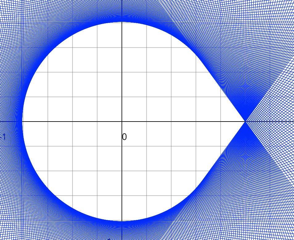
Figure 1. $n=4$, $m=4$, $k=1$, $\alpha=0$, $\beta=1$

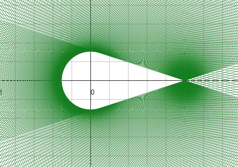
Figure 2. $n=4$, $m=4$, $k=2$, $\alpha=0$, $\beta=1$

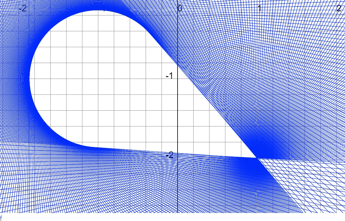
Figure 3. $n=5$, $m=5$, $k=1$, $\alpha=-1-i$, $\beta=1-2i$

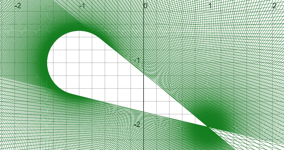
Figure 4. $n=5$, $m=5$, $k=2$, $\alpha=-1-i$, $\beta=1-2i$

Remark 3.9.

When $m<n$, a new radius, $\cos\psi_{k,m}$, makes an appearance if $m<k\leq n/2$. In Fig. 4 this does not occur, but it does in Fig. 6, for $\Lambda_{2}(J_{5}(-1-i)\oplus(1-2i))$. This is a case where $\Lambda_{k}(T)$ is not a convex combination of certain (higher) numerical ranges of its direct summands. In Fig. 6 we can see a representation of the (areas corresponding to the) sets $D_{k}$—in blue—and $C_{k,m}$—in red.

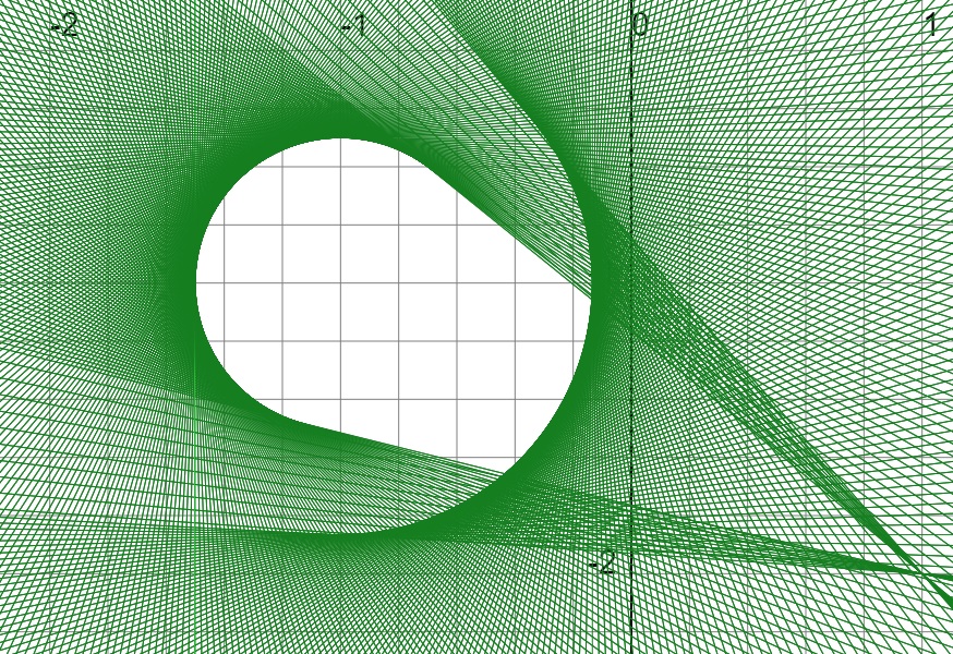
Figure 5. $n=5$, $m=1$, $k=2$, $\alpha=-1-i$, $\beta=1-2i$

Figure 6. $n=5$, $m=1$, $k=2$, $\alpha=0$, $\beta=\sqrt{2}$

4. Remarks and Applications

Remark 4.1.

The results in Theorem 3.7 and the accompanying images show concrete examples of the following result of Chang, Gau, and Wang (here $W_{k}(T)$ denotes Halmos’ higher numerical range):

Proposition 4.2 ([20]).

Let $T\in M_{n}(\mathbb{C})$, $k\in\{1,\ldots,n\}$, and $\beta\in\Lambda_{1}(T)$ a point that is a corner. The following statements are equivalent:

1. $\beta$ is a corner of $W_{k}(T)$;

2. $\beta$ is a corner of $\Lambda_{k}(T)$;

3. $T$ is unitarily equivalent to $\beta I_{m}\oplus C$, with $m\geq k$ and $\beta\not\in\Lambda_{1}(C)$.

In particular, Figure 6 shows an example of how the corner $\beta$ can disappear as soon as $k>m$. We note also that in the same example two new corners appear in $\Lambda_{2}(T)$, which are not eigenvalues. Thus there is no Donoghue’s Theorem [21] for $k\geq 2$.

Remark 4.3.

It was proven in [12, Proposition 2.2] that $\Lambda_{k}(T)$ is at most a singleton when $k>n/2$. In the opposite direction, it was shown in [22] that, for $T\in M_{n}(\mathbb{C})$, $\Lambda_{k}(T)$ is always nonempty if $k<n/3+1$, and that it can be empty as early as $k=n/3+1$ in specific examples. The example they give is of a normal operator, and they mention that their example can be perturbed to obtain a non-normal example. Here, Theorem 3.7 gives us a natural non-normal example. Indeed, in the context of Theorem 3.7 their $n$ becomes $n+m$; if $k=(n+m)/3+1$ and $m>(n-3)/2$, then

$$k=\frac{n+m}{3}+1>\frac{n+\frac{n-3}{2}}{3}+1=\frac{n-1}{2}+1=\frac{n+1}{2}.$$

If we also require $m<\tfrac{n+1}{2}$, it follows that $k>m$. Taking $\alpha=0$, $\beta\geq 1$, condition (7) in Theorem 3.7 guarantees that $\Lambda_{k}(J_{n}(0)\oplus\beta I_{m})=\varnothing$. So, for instance, with $n=4$, $m=2$, $k=(n+m)/3+1=3$ we have that $\Lambda_{3}(J_{4}(0)\oplus I_{2})=\varnothing$ and $3=k=6/3+1$. Or, for another example, $\Lambda_{5}(J_{8}(0)\oplus I_{4})=\varnothing$, where $k=5=\frac{12}{3}+1$.

It is also possible to find cases where our examples have nonempty $\Lambda_{k}(T)$ for fairly big $k$. Most examples in the literature of these extreme situations are normal, while—as we mentioned—ours are non-normal. One straightforward way to force the issue is to take very large $m$ (the size of the scalar block) as then we will always have $\Lambda_{k}(T^{0}_{\alpha,\beta})\neq\varnothing$ for $k=m$. But nonempty higher rank numerical ranges for big $k$ appear in our examples even without the need of a big $m$ relative to $n$.

We see from Theorem 3.7 that $\Lambda_{k}(J_{n}(\alpha)\oplus\beta I_{m})=\varnothing$ when $k>m$ and $\cos\psi_{k,m}<0$. The condition $\cos\psi_{k,m}\geq 0$ is $\frac{(k-m)\pi}{n+1}\leq\frac{\pi}{2}$, which we write as $k\leq m+\tfrac{n+1}{2}$. When $n$ is odd and $k=m+\tfrac{n+1}{2}$, we have $\cos\psi_{k,m}=0$. So to have $\Lambda_{k}(J_{n}(\alpha)\oplus\beta I_{m})\neq\varnothing$ with the biggest possible $k$, we need (by 6 and 7 in Theorem 3.7) that $|\beta-\alpha|=0$. We also need $k\leq n+m-1$ as $\Lambda_{n+m}(T^{0}_{\alpha,\beta})=\varnothing$. The condition $m+(n+1)/2\leq m+n-1$ forces $n\geq 3$ and the equality can only occur when $n=3$.

To see an example of this consider $T=J_{3}(0)\oplus 0_{m}\in M_{3+m}(\mathbb{C})$. If we take $k=2+m$, then $k>m$ and $\cos\psi_{k,m}=0$. As $|\beta-\alpha|=0$, we get from Theorem 3.7 that $\Lambda_{2+m}(T)=\{0\}$. An explicit rank-$(m+2)$ projection $P$ with $P(J_{3}(0)\oplus 0_{m})P=0$ is given by

$$P=\begin{bmatrix}1&0&0\\ 0&0&0\\ 0&0&1\end{bmatrix}\oplus I_{m}.$$

Similarly, consider $n=5$. Now $\tfrac{n+1}{2}=3<4=n-1$. Since $\cos\psi_{4+m}=\cos\tfrac{4\pi}{6}=-\tfrac{1}{2}$, we have that $\Lambda_{4+m}(J_{5}(\alpha)\oplus\beta I_{m})=\varnothing$ for any $\alpha,\beta$. But $\Lambda_{3+m}(J_{5}(0)\oplus 0_{m})=\{0\}$ by case 4 in Theorem 3.7. As $\Lambda_{3}(J_{5}(0))=\{0\}$, it is enough to find a projection $Q\in M_{5}(\mathbb{C})$, of rank 3, such that $QJ_{5}(0)Q=0$. An easy concrete realization of such $Q$ is

$$Q=\begin{bmatrix}1&0&0&0&0\\ 0&0&0&0&0\\ 0&0&1&0&0\\ 0&0&0&0&0\\ 0&0&0&0&1\\ \end{bmatrix}.$$

If we put $P=Q\oplus I_{m}$, then $P$ is a projection of rank $3+m$ and we have $P(J_{5}(0)\oplus 0_{m})P=0_{5+m}$.

In general, if $n=2\ell+1$, then $\Lambda_{\ell+1}(J_{2\ell+1}(0))=\{0\}$ and we can form $Q=\sum_{j=1}^{\ell+1}E_{2j-1,2j-1}$ to get a rank-$(\ell+1)$ projection $Q$ with $QJ_{2\ell+1}(0)Q=0$. Indeed,

$$QJ_{2\ell+1}(0)Q=\sum_{j,h=1}^{\ell+1}\sum_{k=1}^{2\ell+1}E_{2j-1,2j-1}E_{k,k+1}E_{2h-1,2h-1}=0,$$

since $k$ and $k+1$ cannot be both odd. Then $P=Q\oplus I_{m}$ is a rank-$(\ell+1+m)$ projection with $P(J_{2\ell+1}(0)\oplus 0_{m})P=0_{2\ell+1+m}$, showing explicitly (note that it also follows directly from case 6 in Theorem 3.7) that $\Lambda_{\ell+1+m}(J_{2\ell+1}(0)\oplus 0_{m})=\{0\}$. For $k=\ell+2+m$, we have $\cos\psi_{\ell+2+m,m}=\cos\frac{(\ell+2)\pi}{2\ell+2}<0$, so $\Lambda_{\ell+2+m}(J_{2\ell+1}(0)\oplus 0_{m})=\varnothing$ by case 7 in Theorem 3.7.

Question 4.4.

The only way to have $T\in M_{n}(\mathbb{C})$ with $\Lambda_{n}(T)\neq\varnothing$ is to have $T=\beta I$ for some $\beta$. We see from Remark 4.3 that $\Lambda_{2+m-1}(J_{2}(0)\oplus 0_{m})\neq\varnothing$, and $\Lambda_{3+m-1}(J_{3}(0)\oplus 0_{m})\neq\varnothing$, while $\Lambda_{n+m-1}(J_{n}(\alpha)\oplus\beta I_{m})=\varnothing$ for $n\geq 4$ and any $\alpha,\beta$. This suggests the following question: Given $n\geq 4$, does there exist non-normal $T\in M_{n}(\mathbb{C})$ with $\Lambda_{n-1}(T)\neq\varnothing$? The existence of a normal irreducible $T\in M_{n}(\mathbb{C})$, not a scalar multiple of the identity, with $\Lambda_{n-1}(T)\neq\varnothing$ was established in [22, Theorem 3].

Remark 4.5.

The following result due to J. Anderson. There is a nice proof in [23], where it is attributed to Pei-Yuan Wu (who published more general results in [24]). An infinite-dimensional version appears in [25], where the authors briefly discuss the story of the theorem and the various proofs that have been published.

Proposition 4.6 (J. Anderson).

Let $n\geq 2$ and $T\in M_{n}(\mathbb{C})$. Let $\alpha\in\mathbb{C}$, $r>0$. If $\Lambda_{1}(T)\subset B_{r}(\alpha)$ and $|\Lambda_{1}(T)\cap\partial B_{r}(\alpha)|\geq n+1$, then $\Lambda_{1}(T)=B_{r}(\alpha)$.

One might be tempted to try to think of $\Lambda_{k}(T)$ as the numerical range of some amplification/dilation of $T$. Actually, this works for some of our examples: for instance, we see from Theorem 3.7 that $\Lambda_{2}(J_{5}(0)\oplus I_{4})=\operatorname{conv}(B_{1/2}(0)\cup\{1\})=\Lambda_{1}(J_{2}(0)\oplus I_{4})$. But, at the same time Proposition 4.6, together with some of our examples above show that this is not the case in general. Concretely, if we look at the example from Fig. 6, namely $\Lambda_{2}(J_{n}(-1-i)\oplus(1-2i)I_{1})$, we can see that the whole set is contained in the disk of radius $\cos\psi_{2}=\cos\tfrac{(2-1)\pi}{5+1}=\tfrac{\sqrt{3}}{2}$ centered at $-1-i$, and it shares a nontrivial part of the arc; thus Proposition 4.6 implies that $\Lambda_{2}(J_{n}(-1-i)\oplus(1-2i)I_{1})$ is not the numerical range of any matrix. We also conclude that there is no analogue of Proposition 4.6 for any $k>1$.

Remark 4.7.

An easy and well-known property of the higher numerical range is that

(4.1) $$\Lambda_{k}(T\oplus S)\supset\Lambda_{k}(T)\cup\Lambda_{k}(S).$$

As $\Lambda_{k}(T\oplus S)$ is convex, it will always contain $\operatorname{conv}\{\Lambda_{k}(T)\cup\Lambda_{k}(S)\}$. But it is often the case that the inclusion is strict, as for instance when $\Lambda_{k}(T\oplus T)$ with $T\in M_{n}(\mathbb{C})$ and $k>n$. In Theorem 3.7, case 2, we see that the inclusion (4.1) can be an equality for several values of $k$; indeed, under the conditions of case 2 we have $\Lambda_{k}(J_{n}(\alpha))=B_{\cos\phi_{k}}(\alpha)$, and $\Lambda_{k}(\beta I_{m})=\{\beta\}$ and $\Lambda_{k}(J_{n}(\alpha)\oplus\beta I_{m})=\operatorname{conv}\Lambda_{k}(J_{n}(\alpha))\cup\Lambda_{k}(\beta I_{m})$.

Remark 4.8.

If $T_{1},T_{2}$ are unitarily equivalent, then $\Lambda_{k}(T_{1})=\Lambda_{k}(T_{2})$ for all $k$. The converse is known to be false in general [26]. The class of matrices of the form $J_{n}(\alpha)\oplus\beta I_{m}$ is rigid enough that the family of higher rank numerical ranges characterizes unitary equivalence (equality, actually). Namely,

Corollary 4.9.

Let $T_{j}=J_{n_{j}}(\alpha_{j})\oplus\beta_{j}I_{m_{j}}$, $j=1,2$, such that $n_{1}+m_{1}=n_{2}+m_{2}$ and such that for all $k$ we have $\Lambda_{k}(T_{1})=\Lambda_{k}(T_{2})$. Then $T_{1}=T_{2}$.

Proof.

We refer to the cases that appear in the table in Theorem 3.7. Consider first $k=1$. From Theorem 3.7 we know that both $T_{1},T_{2}$ fall in the same of cases 1 or 2. In both cases we have that part of the boundary of $\Lambda_{1}(T_{j})$ is an arc of a circle of radius $\cos\phi_{k}$ centered at $\alpha_{j}$ (the number $\cos\phi_{k}$ is in principle different for $T_{1}$ and $T_{2}$, but since we are arguing that in this case it is the same for both, there is no need for a particular notation for that). Thus $\alpha_{1}=\alpha_{2}$, and looking at the cosines we need $1/(n_{1}+1)=1/(n_{2}+1)$, so $n_{1}=n_{2}$ and then $m_{1}=m_{2}$.

If any of cases 2 or 3 arise for some $k$, as the (extensions of the, in case 3) line segments intercept at $\beta$ (recall that $R^{\psi}_{|\beta-\alpha|,k}=\alpha+e^{i\psi}R_{|\beta-\alpha|,k}$ and $\alpha+e^{i\psi}|\beta-\alpha|=\beta$), we get that $\beta_{1}=\beta_{2}$.

If neither case 2 nor 3 arises, we are in case 1 for all $1\leq k\leq n/2$ for both $T_{1}$ and $T_{2}$. So $|\beta_{1}-\alpha|$,$|\beta_{2}-\alpha|\leq\cos\phi_{k}<1$ for all such $k$. Thus

(4.2) $$|\beta_{j}-\alpha|\leq\cos\frac{\lfloor n/2\rfloor}{n+1}\,\pi.$$

If case 6 arises for some $k$, we get $\beta_{1}=\beta_{2}$. And case 6 will always arise in the presence of (4.2); for if case 7 occurs already for $k=\lfloor n/2\rfloor+1$, we have $m_{j}<\lfloor n/2\rfloor+1$ so

$$k-m_{j}=\lfloor\tfrac{n}{2}\rfloor+1-m_{j}\leq\lfloor\tfrac{n}{2}\rfloor$$

and thus

$$|\beta_{j}-\alpha|>\cos\psi_{k,m_{j}}=\cos\frac{\lfloor n/2\rfloor+1-m_{j}}{n+1}\,\pi\geq\cos\frac{\lfloor n/2\rfloor}{n+1}\,\pi\geq|\beta_{j}-\alpha|,$$

a contradiction. ∎

5. Acknowledgements

This work has been supported in part by the Discovery Grant program of the Natural Sciences and Engineering Research Council of Canada grant RGPIN-2015-03762.

References

- [1] T. Ando. Structure of operators with numerical radius one. Acta Sci. Math. (Szeged), 34:11–15, 1973.
- [2] K. Bickel and P. Gorkin. Compressions of the shift on the bidisk and their numerical ranges. J. Operator Theory, 79(1):225–265, 2018.
- [3] H.-L. Gau and C.-K. Li. -isomorphisms, Jordan isomorphisms, and numerical range preserving maps. Proc. Amer. Math. Soc., 135(9):2907–2914, 2007.
- [4] T. Kato. Perturbation theory for linear operators. Classics in Mathematics. Springer-Verlag, Berlin, 1995. Reprint of the 1980 edition.
- [5] D. W. Kribs, A. Pasieka, M. Laforest, C. Ryan, and M. P. da Silva. Research problems on numerical ranges in quantum computing. Linear Multilinear Algebra, 57(5):491–502, 2009.
- [6] C.-K. Li and N.-S. Sze. Canonical forms, higher rank numerical ranges, totally isotropic subspaces, and matrix equations. Proceedings of the American Mathematical Society, 136(9):3013–3023, 2008.
- [7] C.-K. Li, B.-S. Tam, and P. Y. Wu. The numerical range of a nonnegative matrix. Linear Algebra Appl., 350:1–23, 2002.
- [8] C.-K. Li. Inequalities relating norms invariant under unitary similarities. Linear and Multilinear Algebra, 29(3-4):155–167, 1991.
- [9] M. N. Spijker. Numerical ranges and stability estimates. Applied Numerical Mathematics, 13(1-3):241–249, 1993.
- [10] R. Horn and R. Johnson, Charles. Topics in matrix analysis. Cambridge University Press, Cambridge, UK, 1994.
- [11] P. R. Halmos. A Hilbert space problem book, volume 19 of Graduate Texts in Mathematics. Springer-Verlag, New York, second edition, 1982. Encyclopedia of Mathematics and its Applications, 17.
- [12] M.-D. Choi, D. W. Kribs, and K. Życzkowski. Higher-rank numerical ranges and compression problems. Linear algebra and its applications, 418(2–3):828–839, 2006.
- [13] H. J. Woerdeman. The higher rank numerical range is convex. Linear Multilinear Algebra, 56(1-2):65–67, 2008.
- [14] M.-D. Choi, J. A. Holbrook, D. W. Kribs, and K. Zyczkowski. Higher-rank numerical ranges of unitary and normal matrices. Operators and Matrices, 1(3):409–426, 2007.
- [15] H. Gaaya. On the higher rank numerical range of the shift operator. J. Math. Sci. Adv. Appl., 13(1):1–19, 2012.
- [16] M. Adam, A. Aretaki, and I. M. Spitkovsky. Elliptical higher rank numerical range of some Toeplitz matrices. Linear Algebra Appl., 549:256–275, 2018.
- [17] M.-T. Chien and H. Nakazato. The boundary of higher rank numerical ranges. Linear Algebra Appl., 435(11):2971–2985, 2011.
- [18] U. Haagerup and P. de la Harpe. The numerical radius of a nilpotent operator on a Hilbert space. Proc. Amer. Math. Soc., 115(2):371–379, 1992.
- [19] J.-L. de Lagrange. Recherches sur la nature et la propagation du son. Miscellanea Taurinensia, 1:39–148, 1759.
- [20] C.-T. Chang, H.-L. Gau, and K.-Z. Wang. Equality of higher-rank numerical ranges of matrices. Linear Multilinear Algebra, 62(5):626–638, 2014.
- [21] W. F. Donoghue. On the numerical range of a bounded operator. The Michigan Mathematical Journal, 4(3):261–263, 1957.
- [22] C.-K. Li, Y.-T. Poon, and N.-S. Sze. Condition for the higher rank numerical range to be non-empty. Linear Multilinear Algebra, 57(4):365–368, 2009.
- [23] B.-S. Tam and S. Yang. On matrices whose numerical ranges have circular or weak circular symmetry. Linear Algebra Appl., 302/303:193–221, 1999. Special issue dedicated to Hans Schneider (Madison, WI, 1998).
- [24] P. Y. Wu. Numerical ranges as circular discs. Appl. Math. Lett., 24(12):2115–2117, 2011.
- [25] H.-L. Gau and P. Wu. Anderson’s theorem for compact operators. Proceedings of the American Mathematical Society, 134(11):3159–3162, 2006.
- [26] H.-L. Gau and P. Y. Wu. Higher-rank numerical ranges and Kippenhahn polynomials. Linear Algebra Appl., 438(7):3054–3061, 2013.