The Hubble Legacy Field GOODS-S Photometric Catalog

Abstract

This manuscript describes the public release of the Hubble Legacy Fields (HLF) project photometric catalog for the extended GOODS-South region from the Hubble Space Telescope (HST) archival program AR-13252. The analysis is based on the version 2.0 HLF data release that now includes all ultraviolet (UV) imaging, combining three major UV surveys. The HLF data combines over a decade worth of 7475 exposures taken in 2635 orbits totaling 6.3 Msec with the HST Advanced Camera for Surveys Wide Field Channel (ACS/WFC) and the Wide Field Camera 3 (WFC3) UVIS/IR Channels in the greater GOODS-S extragalactic field, covering all major observational efforts (e.g., GOODS, GEMS, CANDELS, ERS, UVUDF and many other programs; see Illingworth et al 2019, in prep). The HLF GOODS-S catalogs include photometry in 13 bandpasses from the UV (WFC3/UVIS F225W, F275W and F336W filters), optical (ACS/WFC F435W, F606W, F775W, F814W and F850LP filters), to near-infrared (WFC3/IR F098M, F105W, F125W, F140W and F160W filters). Such a data set makes it possible to construct the spectral energy distributions (SEDs) of objects over a wide wavelength range from high resolution mosaics that are largely contiguous. Here, we describe a photometric analysis of 186,474 objects in the HST imaging at wavelengths 0.2–1.6$\mu$m. We detect objects from an ultra-deep image combining the PSF-homogenized and noise-equalized F850LP, F125W, F140W and F160W images, including Gaia astrometric corrections. SEDs were determined by carefully taking the effects of the point-spread function in each observation into account. All of the data presented herein are available through the HLF website (https://archive.stsci.edu/prepds/hlf/).

1. Introduction

Our current understanding of the formation and evolution of galaxies with cosmic time is driven by large, statistical samples that span a broad range of multi-wavelength observations. The deepest and highest resolution observations exploring the peak epoch of star formation in our universe are those from the Hubble Space Telescope (HST; e.g., Giavalisco et al., 2004; Scoville, 2007; Grogin et al., 2011; Koekemoer et al., 2011; Momcheva et al., 2016). When combining HST with the deepest ground-based observations and Spitzer Space Telescope, surveys enable the measurement of fundamental galaxy properties for tens of thousands of extragalactic sources. HST alone has pushed galaxy studies into uncharted territory (e.g., McLeod et al., 2015; Oesch et al., 2016).

The scientific returns from extragalactic legacy surveys are maximized when data sets are combined in a homogeneous way. To this end, we undertake the construction of a photometric catalog based solely on all high resolution HST imaging taken in the greater GOODS-S extragalactic field to date. While the future inclusion of Spitzer/IRAC and ground-based ancillary data will continue to improved the measured photometric redshifts and stellar population parameters, this work serves as a necessary albeit incremental step towards a comprehensive final catalog of the GOODS-S extragalactic legacy field. The extended GOODS-S/CDF-S region has the largest ensemble of HST imaging data of any area of the sky. The equivalent of approximately 75% of an HST cycle has now been committed to imaging this area through more than 30 different programs. In total, there is 6.3 Msec of HST on-target time through 7475 exposures taken over 2635 orbits of ACS, WFC3/IR and WFC3/UVIS imaging. A summary of all programs is found in Table 1.

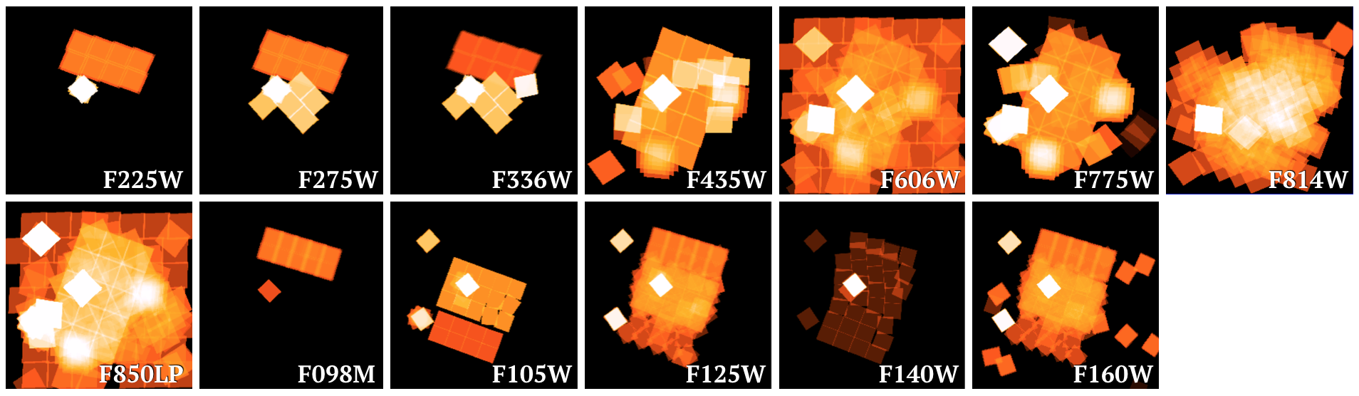
Figure 1.— The HLF-GOODS-S dataset weight maps outlining the footprints for the three WFC3/UVIS, five ACS/WFC, and five WFC3/IR filters. White represents the deepest data corresponding to the footprint of the HUDF/XDF.

The catalog is based on the version 2.0 (v2.0) release of the Hubble Legacy Field GOODS-S (HLF-GOODS-S). Figure 1 shows the coverage for the thirteen HST filters included in the photometric catalog. The v2.0 version of HLF-GOODS-S updates the v1.5 version with the inclusion of all of the available UV imaging data. The three UV surveys added constitute a substantial body of data, totaling 213 orbits of HST WFC3/UVIS imaging, or about 0.5 Msec of observations: the Early Release Science (ERS) observations (Windhorst et al., 2011), the UltraViolet Ultra-Deep Field (UVUDF) dataset (Teplitz et al., 2013; Rafelski et al., 2015), the Hubble Deep UltraViolet (HDUV) legacy dataset (Oesch et al., 2018), as well as additional F336W imaging data (Vanzella et al., 2016). A summary of these UV programs and the details of all other datasets from v1.5 can be found in Table 1. The orbit values listed are computed from the total exposure time in each program/filter, where 1 orbit equals 2400s of exposure time. The UV datasets were updated and astrometrically-matched to the v1.5 release of the HLF-GOODS-S. The ERS dataset of Windhorst et al. (2011) required a full processing as high level science products are not available on the Mulkulsi Archive for Space Telescopes. The steps that were taken to assemble the HST UV, optical and near-IR data, including details of the data reduction and astrometric analysis, can be found in Illingworth et al. (2016, 2019, in prep). Here, we describe the details of the source detection, PSF homogenization, and catalog construction. We provide the homogenized set of images that are used in this paper to the community, in addition to the photometric catalog.

The structure of this manuscript is as follows. In Section 2.2 and 2.3, we describe the additional background subtraction and the source detection, respectively. Section 2.3 details the PSF matching of the different resolution images, and Section 2.4 the general layout of the photometric catalogs themselves. We present basic internal and external diagnostic plots to verify quality and consistency in Section 3. Section 4 contains a general overview of the public release of the HLF GOODS-S photometric catalog.

In this manuscript, all magnitudes are in the AB system and we assume a $\Lambda$CDM cosmology with $\Omega_{\mathrm{M}}=0.3$, $\Omega_{\Lambda}=0.7$, and $\mathrm{H_{0}}=70$ km s^-1 Mpc^-1.

Table 1Hubble Space Telescope programs contributing to the HLF-GOODS-South

Program ID	Program	Filter(s)	Orbit(s)
9352	$\cdots$	F606W/F775W/F850LP	2/2/12
9425	GOODS	F435W/F606W/F775W/F850LP	45/33/33/68
9480	$\cdots$	F775W	12
9488	$\cdots$	F775W/F850LP	3/2
9500	GEMS	F606W/F850LP	56/60
9575	$\cdots$	F775W	3
9793	GRAPES	F606W	1
9803	HUDF-NICMOS	F435W/F606W/F775W/F850LP	17/19/35/52
9978	HUDF	F435W/F606W/F775W/F850LP	52/54/139/137
9984	$\cdots$	F775W	1
10086	HUDF	F435W/F606W/F775W/F850LP	4/2/6/8
10189	PANS	F435W/F606W/F775W/F850LP	1/5/7/17
10258	$\cdots$	F606W/F775W/F850LP	11/1/24
10340	PANS	F606W/F775W/F850LP	2/12/48
10530	$\cdots$	F606W	5
10632	HUDF-P1/P2	F606W/F775W/F850LP	18/45/138
11144	$\cdots$	F125W/F850LP	1/1
11359	ERS	F225W/F275W/F336W/F814W/F098M/F125W/F140W/F160W	19/19/9/17/21/21/0/21
11563	HUDF09	F435W/F606W/F775W/F814W/F850LP/F105W/F125W/F160W	18/42/40/30/79/50/77/98
12007	$\cdots$	F606W	1
12060	CANDELS	F606W/F814W/F850LP/F105W/F125W/F160W	11/31/14/61/2/2
12061	CANDELS	F814W/F850LP/F125W/F160W	70/9/42/44
12062	CANDELS	F606W/F814W/F850LP/F125W/F160W	2/50/12/33/34
12099	CANDELS-SN	F435W/F606W/F775W/F814W/F850LP/F098M/F105W/F125W/	1/2/1/19/4/1/1/10/1/8
		F140W/F160W
12177	3D-HST	F814W/F140W	8/13
12461	CANDELS-SN	F125W/F160W/F435W/F606W/F814W/F850LP	4/1/0/1/2/2
12498	HUDF12	F105W/F140W/F160W/F814W	83/34/30/135
12534	UVUDF	F225W/F275W/F336W/F435W/F606W/F775W/F814W/F850LP	18/17/16/73/5/2/12/2
12866	$\cdots$	F160W/F814W	13/11
12990	$\cdots$	F160W	1
13779	$\cdots$	F105W/F435W/F606W/F814W	8/4/2/4
13872	HDUV	F275W/F336W/F435W	50/45/47
14088	$\cdots$	F336W	20

2. Photometry

We construct the HLF photometric catalog as detailed below, closely following the techniques discussed in depth in Skelton et al. (2014) and Shipley et al. (2018). In summary, we use a deep noise-equalized combination of the four HST bands (F850LP, F125W, F140W, F160W) for detection. 12 HST bandpasses (F225W, F275W, F336W, F435W, F606W, F775W, F814W, F850LP, F098M, F105W, F125W, and F140W) are each convolved to the F160W point-spread function (PSF) in order to measure consistent colors across all wavebands. For this entire analysis, we use the v2.0 release 60 mas pixel scale mosaics. Aperture photometry was performed in dual-image mode using Source Extractor (Bertin & Arnouts, 1996) on the background-subtracted, homogenized images using a small aperture of diameter of 0.7^′′ that maximizes the signal-to-noise of the resulting aperture photometry.

2.1. Background Subtraction

With the v2.0 mosaics for the optical and near-infrared filters (F435W–F160W) and the ultraviolet (F225W–F336W), we first do an additional sky subtraction to remove any excess light previously missed during the initial routine sky subtraction performed during the data reduction. The sky subtraction is performed using Source Extractor (SExtractor; Bertin & Arnouts, 1996), using a Gaussian interpolation of the background with an adopted mesh size of 64 pixels and a 7 pixel median filter size. The result of this sky subtraction is on the order of a few hundredths of a percent per pixel, a minimal correction but necessary to improve the overall homogeneity of the background.

2.2. Source Detection

We create a detection image that is a noise-equalized version of the mosaics combining one ACS (F850LP) with three WFC3 bands (F125W, F140W, F160W) by multiplying the PSF-matched science images (see details in Section 2.3) by the square root of the inverse variance map. These four noise-equalized images are then coadded to form an ultra-deep detection image. Such a methodology has been adopted in several earlier surveys: e.g., NMBS (Whitaker et al., 2011), 3D-HST (Skelton et al., 2014), and HFF-DeepSpace (Shipley et al., 2018). The decision to include F850LP stems from the wide field coverage in this filter that extends to significantly larger area than the nominal WFC3 footprint. Our methodology adopts an extremely deep detection image while also explicitly taking into account variations in the weight across the mosaics. This variation in weight is a natural consequence of combining many different observing programs with unique science goals into single mosaics. We use a detection and analysis threshold of 1.8$\sigma$ and 1.4$\sigma$, respectively, and require a minimum area of 14 pixels for detection. The deblending threshold is set to 32, with a minimum contrast parameter of 0.0001. A Gaussian filter of 7 pixels is used to smooth the images before detection. The detection parameters were optimized such that the settings are a compromise between deblending neighboring objects while minimizing dividing larger objects into multiple components. Moreover, visual inspection confirms that the input SExtractor parameters find all faint objects in the ultra-deep detection images, while limiting the number of spurious detections.

The resulting objects detected are not cleaned for spurious detections within SExtractor itself, as this may cause subtle problems with the segmentation maps. Instead, we clean the photometry in post-processing. Any object residing in a region with a weight less than 1% of the 95th percentile weight is identified as problematic and the photometry of the respective band is fixed to a value of -99. This represents 30% of the total catalog in the F160W and F850LP filters.

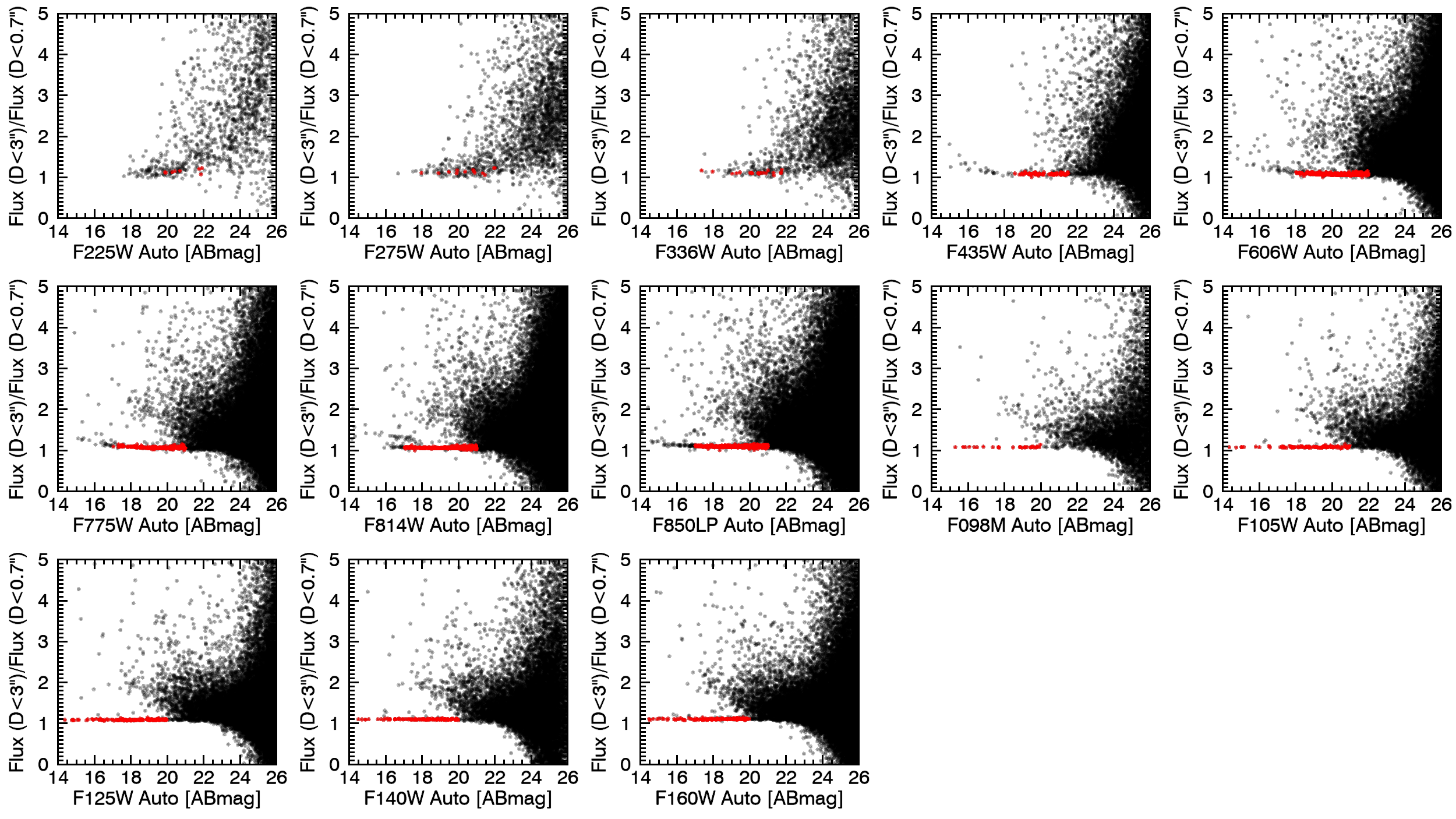
Figure 2.— Point sources have a ratio of flux within a larger 3^′′ diameter circular aperture relative to a small 0.7^′′ diameter aperture close to unity. We can therefore cleanly identify bright, unsaturated stars (red) to generate empirical PSFs in each filter on the basis of this ratio.

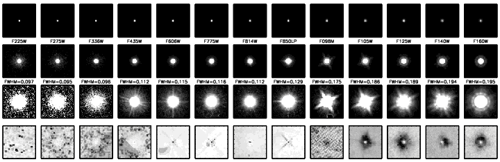
Figure 3.— (Top) empirical point spread functions derived from bright stars selected across each mosaic, displayed at different stretch levels from the top to third row to highlight various features. (Bottom) stacked weight maps for the stars used to derive the PSF.

2.3. Point Spread Function Homogenization

In order to measure accurate colors, we need to PSF-match the HST ACS and WFC3 images to the filter with the broadest FWHM (the F160W filter in this dataset) prior to performing aperture photometry. To do so, empirical PSFs are created for each HST image by stacking isolated unsaturated stars selected from across the mosaic. An initial sample of stars are identified on the basis of the ratio of their fluxes within a large 3^′′ diameter aperture relative to a small 0.7^′′ diameter aperture. Bright, unsaturated stars can be cleanly identified from this ratio (see Figure 2). The number of stars identified ranges from a minimum of 29 in F098M to a maximum of 353 in F606W, with a more typical value of 100–200 stars. We extract 5^′′$\times$5^′′ regions around each star, recentering and masking nearby pixels that are either associated with nearby objects according to the segmentation map, or 5$\sigma$ above the local noise. All stars that either require $>$1.5 pixel shifts to recenter or fail altogether are additionally rejected at this stage. From this parent sample, we perform a visual inspection to remove any remaining problematic stars. A few examples of removed sources include cases where the central pixels were masked incorrectly as cosmic rays, the objects fell on the edge of the detector, or the object was severely contaminated by nearby bright objects. Most stars automatically identified in the UVIS F225W–F336W filters fell on the edges of the detector and therefore failed the earlier recentering algorithm. For example, after this step, the total number of useable stars reduced from 100s to 8–21 in F225W-F336W. The median local background is measured on the final stacked image for pixels located at a radius of 4–5^′′. Though often negligible, we subtract this background correction. We do not attempt to take into account variations with chip position, as the mosaics comprise multiple pointings with different orientations and overlap. As noted by Skelton et al. (2014), we expect such differences to be small.

Figure 3 shows the empirical PSFs and weight maps generated from the procedure outlined herein based on the v2.0 HLF project mosaics. Note that there may be some residual false clipping of the central pixels of the ACS images due to the cosmic ray rejection adopted during the data reduction. Evidence for this can be seen in the depression in the centers of the stacked ACS weight maps for bright stars. One reason this happens in the ACS images is that the dataset itself has been taken over an approximately 12 year timespan. Over this epoch, the positions of some stars have changed. The central pixels will therefore get clipped, as they are no longer aligned due to this proper motion. The top row in Figure 3 emphasizes the core of the PSF where most of the power resides, whereas the contrast in middle and bottom rows highlights the first Airy ring (∼0.5%) and the diffraction spikes (∼0.1%), respectively. A single orientation would contain four diffraction spikes resulting from the secondary mirror assembly. We see in some cases here a much larger number of diffraction spikes (especially for WFC3) due to the broad range of orientations that comprise the mosaiced data. The trade off of the aggressive deblending adopted on the ultra-deep detection image is that the diffraction spikes and first Airy ring around bright stars will often be identified as a separate object from the star itself. This can be seen in the weight maps, with the masked regions outlining these PSF features. Note however that these are very faint features and the PSF remains robust given the large number of stars contributing to the stack in the NIR; the point of the PSF homogenization is to match the light profiles across all of the filters, which we will show in the next section is good to the $<$0.5% level at all radii.

Figure 4 shows the curve of growth, defined as the fraction of light enclosed as a function of aperture size, for each of the PSFs, normalized at 2^′′. The top panel of Figure 4 shows the growth curves from the empirical PSFs presented in Figure 3, whereas the bottom panel shows the results after convolving each PSF to match F160W. We derive the convolution kernel by fitting a series of Gaussian-weighted Hermite polynomials to the Fourier transform of the empirical PSFs (Figure 5). This methodology yields PSFs with almost indistinguishable growth curves on the scales of interest, agreeing to $<$0.5% at all radii.

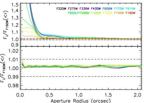
Figure 4.— Growth curves showing the fraction of light enclosed as a function of radius for each HST filter relative to the F160W growth curve before (top) and after (bottom) convolution.

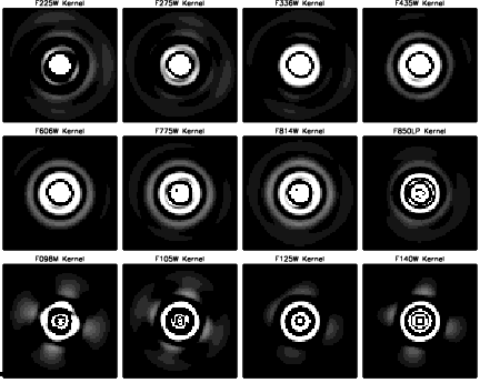
Figure 5.— Convolution kernels derived using a linear combination of Gaussian-weighted Hermite polynomials to match each empirical PSF to the broadest FWHM F160W filter.

Finally, we present a comparison between the encircled energy as a function of aperture provided in the WFC3 handbook relative to our derived F160W empirical PSF in Figure 6. The marginal deviations towards the center of the PSF are not significant, with the curves showing excellent agreement.

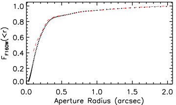
Figure 6.— The fraction of light enclosed as a function of radius for the F160W PSF, relative to the total light within 2^′′. The red dashed line shows the encircled energy as a function of aperture size, also normalized to 2^′′, from the WFC3 handbook. The empirical growth curves (black points) agree well with the theoretical expectation.

2.4. Detection Limits

It is challenging to define completeness limits given our detection methodology and the nature of the HLF dataset, combining a wide range of surveys with dramatically varying depths and coverage between filters. Moreover, defining a single-band magnitude limit is also not entirely meaningful, as it is well known that the detection and completeness limits are a function of galaxy color (e.g., van der Wel et al., 2012). In order to enable users of the HLF GOODS-S dataset to determine the completeness limit of a given sample, we create an effective wavelength map that is equivalent to tracing the wavelength contributing the deepest data at a given location. This effective wavelength map can then be used to determine the magnitude limit for any given object in the mosaic, given the location and $z$-$H$ color, as we describe next.

To create the effective wavelength map for our source detection, we take the convolved weight maps for each of the four filters that combine to make our noise-equalized detection image: $z_{\mathrm{F850LP}}$, $J_{\mathrm{F125W}}$, $JH_{\mathrm{F140W}}$, and $H_{\mathrm{F160W}}$. As the released mosaics maintain the original zeropoints, we first correct all weight maps to a common zeropoint of 25 ABmag. The effective wavelength map is then calculated as follows,

$$\lambda_{e}=\sqrt{\frac{\sum{(w_{X}\lambda_{e,X})^{2}}}{\sum{w_{X}^{2}}}}$$ (1)

where $X$ corresponds to the four filters listed above, $w$ is the weight and $\lambda_{e}$ is the pivot wavelength for each filter. Figure 7 shows the HLF GOODS-S effective wavelength map. The effective wavelength is largely representative of $\sim$1.2$\mu$m across the central field of view, with more extended contiguous coverage at 0.9$\mu$m. We create an effective depth map in a similar manner as above, adding the four weight maps in quadrature, inverting, and taking the square root. Given the effective wavelenth and depth maps, one can simply interpolate the effective wavelength at a given location between 0.92$\mu$m ($z_{\mathrm{F850LP}}$) and 1.54 $\mu$m ($H_{\mathrm{F160W}}$), using that fraction multiplied by the $z$-$H$ color to correct the effective depth in the detection image to the equivalent depth in the $H_{\mathrm{F160W}}$ mosaic. In other words, one can approximate the effective $H_{\mathrm{F160W}}$ depth for any source from its $z$-$H$ color as:

$$\sigma_{lim,H}= \sigma_{lim,\lambda_{e}}+(z-H)\left(\frac{\lambda_{e}-1.54}{1.54-0.92}\right).$$ (2)

For example, let us consider a red object with a $z$-$H$ color of 1.0 in the mosaic outskirts where the effective wavelength of the detection map is 0.9$\mu$m. If the effective depth is 26 ABmag, the depth in $H_{\mathrm{F160W}}$ would be 1 magnitude shallower at 25 ABmag for this source, given the red color but deeper $z$-band mosaic at this location. On the other hand, a blue object with a $z$-$H$ color of -1.0 in the same region would instead have an effective $H_{\mathrm{F160W}}$ depth that is 1 magnitude deeper at 27 ABmag. The effective wavelength and depth maps are both available to users within the larger HLF GOODS-S photometric catalog public release.

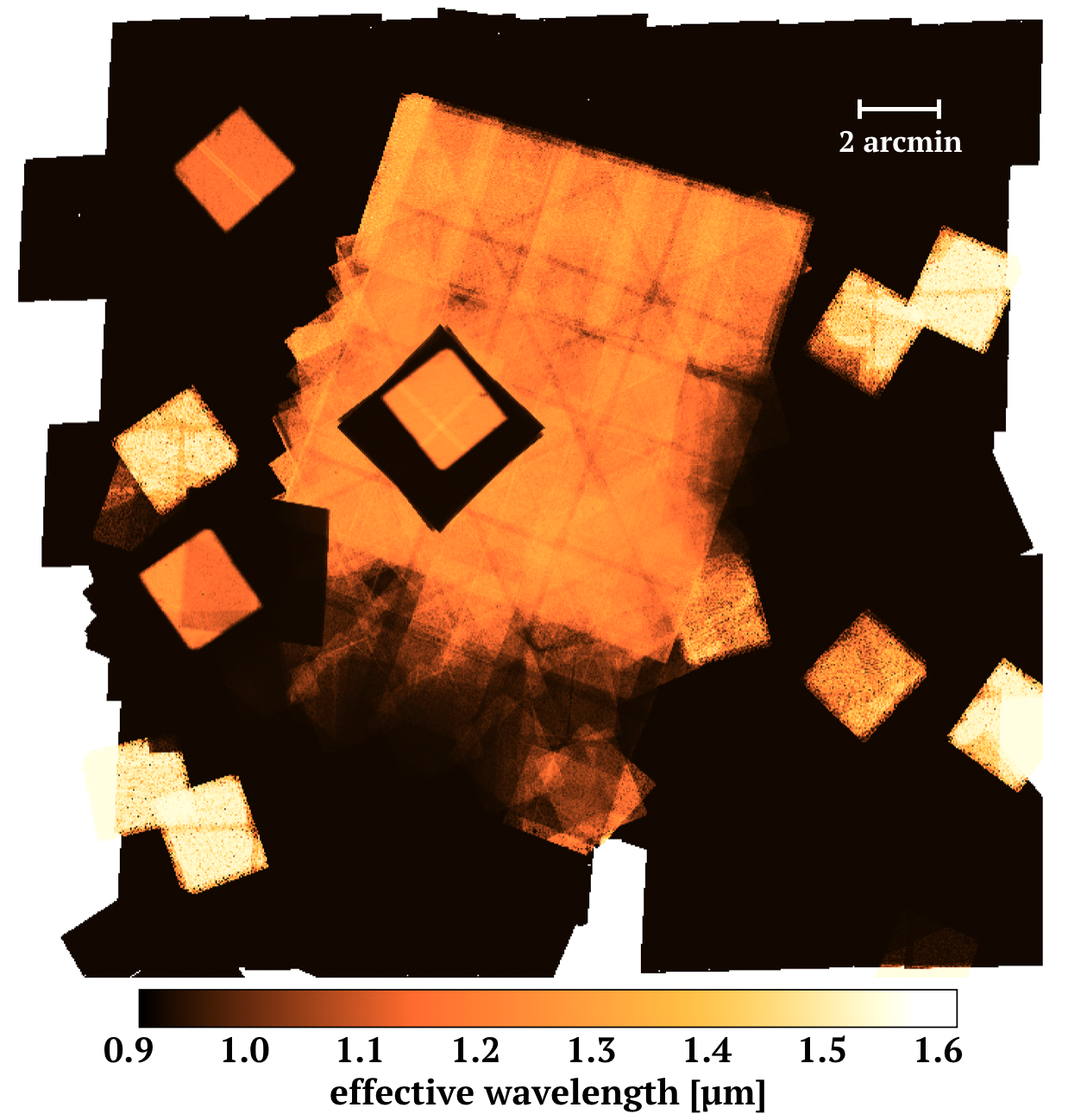
Figure 7.— Map of the effective wavelength of the detection image, ranging from the $z_{\mathrm{F850LP}}$ at 0.9$\mu$m (black) to $H_{\mathrm{F160W}}$ at 1.5$\mu$m (yellow/white). The filter with the deepest data (largest weights) will dominate the effective wavelength map, which varies across the field of view due to the heterogeneous nature of the HLF GOODS-S combined dataset.

2.5. Photometric Catalogs

2.5.1 Aperture Photometry

Our aperture photometry methodology closely follows that of Skelton et al. (2014). We therefore briefly summarize the main steps followed here and note any different assumptions we have adopted, but defer the reader to Section 3.4 of Skelton et al. (2014) for additional details. SExtractor is run in dual-image mode, where the ultra-deep noise-equalized input image is used for detection (see Section 2.2) and the PSF-matched HST image and corresponding convolved weight map are used for the aperture photometry. No further background subtraction is needed at this stage. We perform photometry within a 0.7^′′ diameter circular aperture in all the HST bands. This relatively small aperture optimizes the photometry signal-to-noise ratio (SNR) for point sources (and small higher redshift galaxies), as discussed in Whitaker et al. (2011) and later adapted for HST resolution data in Skelton et al. (2014). This aperture diameter was identified by taking a ratio of the flux enclosed from the growth curve analysis relative to the analogous error analysis (“empty apertures”, as described in Section 2.5.3) as a function of aperture diameter. The SNR peaks around 0.7^′′ for HST quality data, thus optimizing the color photometry. The adopted aperture corresponds to a physical radius of 2.6-3.0 kpc at $z$$\gtrsim$1, which is smaller than the effective radius for the majority of galaxies at these redshifts (van der Wel et al., 2014). For the most massive galaxies, especially star-forming, the effective radii will extend beyond the aperture. In these cases (and at $z$$\lesssim$1), we underresolve galaxies and effectively measure central colors only. The decision to adopt a relatively small aperture will therefore not be optimal for certain parameter spaces. Specific examples include the majority of star-forming galaxies and intermediate/massive (log(M_⋆/M_⊙)$>$10.5) quiescent galaxies at $z$$<$1, intermediate to massive star-forming galaxies (log(M_⋆/M_⊙)$>$10) and massive quiescent galaxies (log(M_⋆/M_⊙)$>$11) at 1$<$$z$$<$2, and intermediate/massive star-forming galaxies (log(M_⋆/M_⊙)$>$10.5) at $z$$\sim$2-3. In these cases, the average effective radii are similar to or larger than the adopted aperture radius due to their more extended light profiles. It is worth noting that the field has not yet converged on the role of color gradients at high redshift. Our methodology assumes a flat gradient by design, which may indeed be a fair assumption at $z$$>$2: Suess et al. (2019) recently showed that color gradients of star-forming and quiescent galaxies are generally flat at $z$$>$2, but color gradients may become more prominent as redshift decreases. In the parameter spaces outlined above, the spectral energy distribution (SED) will be dominated by the central light of the galaxy and may not be representative of the global stellar population properties.

The standard astrometry matches the CANDELS and 3D-HST public releases, but we provide an additional column that corrects for known offsets in astrometry. These astrometric differences were first detected with ALMA data, with offsets in the HUDF of $\delta$ra(deg)=(+0.094$\pm$0.042)/3600 and $\delta$dec(deg)=(-0.262$\pm$0.050)/3600 (see Dunlop et al., 2017; Franco et al., 2018). We adopt an identical approach to Franco et al. (2018), but instead compare positions in the 3D-HST photometric catalogs (which use the same astrometry as the HLF) to the Gaia DR2 catalogs (Gaia Collaboration et al., 2016, 2018). We calculate offsets of $\delta$ra(deg)=(+0.011$\pm$0.08)/3600 and $\delta$dec(deg)=(-0.26$\pm$0.10)/3600, with the equations used to define these corrections listed in Table 2. These offsets are in good agreement with Franco et al. (2018).

The reference band is chosen to be F160W where there is coverage (52% objects) and F850LP otherwise. This decision stems from the wider area coverage of F850LP. We return to this issue when defining columns within the photometric catalog, as there is a significant fraction of the mosaic with only F850LP coverage. The total flux in the reference band is determined by correcting the SExtractor AUTO flux for the amount of light that falls outside of the AUTO aperture. Assuming a point source, this correction can be calculated directly from the growth curves described in Section 2.3. The adopted radius of the AUTO flux corresponds to the Kron radius(Kron, 1980), which encloses rough 90–95% of the total light within a flexible elliptical aperture. Our aperture correction to total flux is therefore the inverse of the fraction of light enclosed within a circular aperture encompassing the same area as the Kron aperture (i.e., the circularized Kron radius). We determine this circularized Kron radius directly from the empirical growth curve for F160W and use the same aperture correction from the reference band to scale all filters. We apply an additional small correction ($<$0.04 mag) to the photometry to account for Galactic extinction in each filter. We interpolate from values given by the NASA Extragalactic Database extinction law calculator, following Skelton et al. (2014) (see Figure 8). All fluxes within the catalog are given as total, with an AB magnitude zero point equal to 25. We also provide the aperture flux in the F160W and F850LP reference bands to allow the user to convert the total fluxes back to consistent color measurements for any band.

Unlike in Skelton et al. (2014), we do not calculate an additional photometric correction to account for any zero point or template mismatch uncertainties. The GOODS-S HLF photometric catalog is strictly comprised of HST filters that typically have minimal zero point offsets calculated. For the case of the 3D-HST GOODS-S photometric catalog, Skelton et al. (2014) calculate zero point offsets ranging from 0.00 to 0.02 mag for all filters but F435W (-0.09 mag). We will return to this point in Section 3.2.

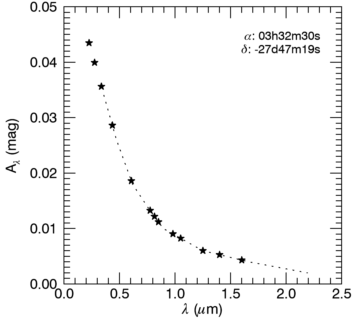
Figure 8.— Galactic extinction in different bandpasses from the NASA Extragalactic Database at the coordinates of the GOODS-S extragalactic field (dotted line; Schlafly & Finkbeiner, 2011). Corrections for Galactic extinction are applied to the HLF GOODS-S photometric catalog by interpolation, where the stars represent the corrections for each HST filter.

2.5.2 Catalog Format

The format of the photometric catalog follows that of the NEWFIRM Medium-Band Survey (Whitaker et al., 2011) and the 3D-HST Survey (Skelton et al., 2014), among others. The total flux and corresponding 1$\sigma$ error for each object is tabulated. The list of column headers and their respective descriptions is located in Table 2. We briefly summarize a few notable columns below.

The weight column for each band quantifies the relative weight for each object compared to the maximum weight for that filter. In practice, the weight is calculated as the ratio of the weight at each object’s position relative to the 95th percentile of the weight map smoothed using a 3 pixel block average. We choose to use the 95th percentile rather than the absolute maximum of the weight map to avoid being affected by extreme values, which is especially important with smaller area ultra deep coverage. For those objects with a weight greater than the 95th percentile, we fix the value to unity in the weight column.

The star_flag column is useful to robustly identify objects that are classified as foreground stars within our own Milky Way galaxy. These point sources are identified on the basis of comparing their SExtractor flux_radius as a function of $H_{\mathrm{F160W}}$ ($z_{\mathrm{F850LP}}$) magnitude (Top panels of Figure 9). Stars are given a value of 1 in the star_flag if their flux radius falls below the selection line (defined in Skelton et al., 2014) and $H_{\mathrm{F160W}}$$<$25 mag column. For all fainter objects with $H_{\mathrm{F160W}}$$>$25 mag, we cannot robustly separate unresolved galaxies from point sources. These objects have star_flag values of 2, and we encourage the user to proceed with caution. While we use the ratio in a large to small aperture as a function of magnitude to identify stars in the PSF-matching section, we ultimately do not adopt this method for defining the star flag as the magnitude limit at which ambiguity of the tight stellar locus sets in is roughly two magnitudes brighter.

The detection_flag column has a value of unity where the F850LP mosaic is adopted as the reference band. In these cases, there is no F160W coverage available. Most often, the broader wavelength coverage in this more extended area is sparse. In the case of no F160W coverage, all structure parameters (e.g., kron_radius, a_image, b_image, flux_radius, etc) are measured from the F850LP mosaic. Furthermore, the total fluxes are derived based on the F850LP bandpass.

Additional noteworthy columns include the wmin_hst column, which indicates for any given object the total number of HST filters with observed flux measurements. The z_spec column cross-matches the positions of each object within a radius of 0.4^′′ with the compilation of spectroscopic redshifts referenced in Skelton et al. (2014) for the GOODS-S field.

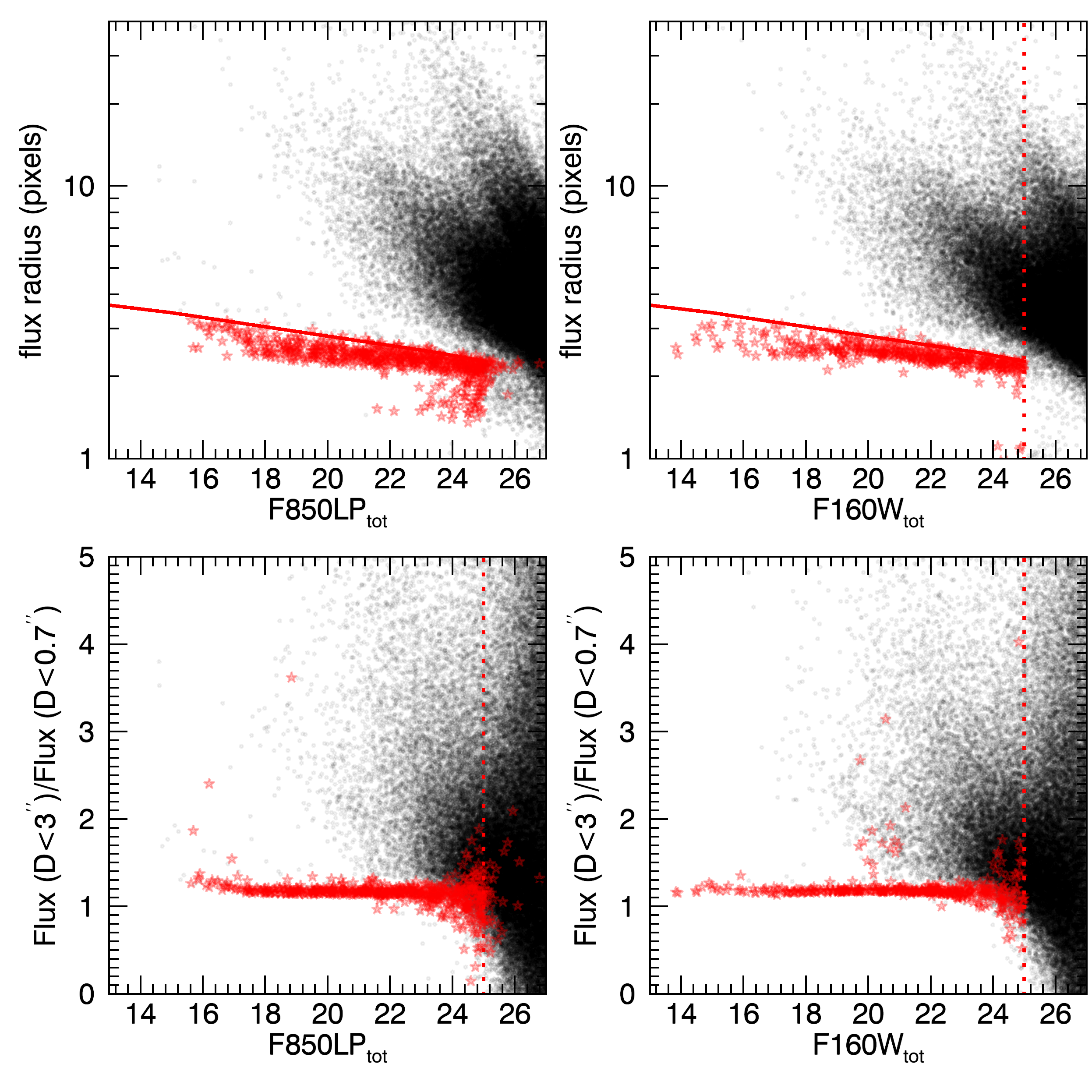
Figure 9.— Top panels: SExtractor’s FLUX_RADIUS against total $z_{\mathrm{F850LP}}$ (left) and $H_{\mathrm{F160W}}$ (right) magnitude. Objects are classified as point sources (red star symbols) in the catalog on the basis of flux radii less than the red line and magnitudes brighter than 25 ABmag (red dotted line). Galaxies and uncertain classifications (with magnitudes $>$25 ABmag) are represented with black symbols. Bottom panels: point sources can also be classified using the ratio of fluxes in a large and small aperture. Although the tightness of the stellar sequence in this ratio at brighter magnitudes allows for a more stringent classification, the separation becomes less clear at fainter magnitudes. The flux ratio was used to select stars for the PSF-matching and kernel fitting (Figure 2).

Finally, perhaps the two most important columns in the catalog are use_f160w and use_f850lp. We provide a flag within the catalog that allows a relatively straightforward selection of galaxies that have photometry of reasonably uniform quality. The default “use” flag (listed as use_f160w in the catalog, to distinguish it from spectroscopic quality flags) is set to 1 if the following criteria are met:

• Not a star, or too faint for reliable star/galaxy separation: star_flag = 0 or star_flag = 2.

• A detection in F160W. To limit the number of false positives, we apply a low SNR cut, requiring f_F160W / e_F160W $>$ 3.

• Sufficient wavelength coverage. We require that a minimum of five filters cover the object. This tends to removes objects on the edges of the mosaics, and in gaps. When running photometric redshift or stellar population synthesis codes, it is common practice to require a similar threshold in the number of bandpasses.

The use_f160w flag selects approximately 39% of all objects in the catalogs. Note that this flag is not very restrictive: for most science purposes further cuts (particularly on magnitude or SNR) are required. Furthermore, we caution that the flag is not 100% successful in removing problematic SEDs. Generally speaking, the overall quality of an SED is higher for galaxies with a higher SNR in the WFC3 bands.

As noted earlier, there exists wider field coverage in the GOODS-S field in the F850LP bandpass. For this reason, we combine this filter into the ultra-deep noise-equalized detection image and adopt it as the reference band where this is no F160W coverage. We include the use_f850lp column to indicate those objects with F850LP coverage. The criteria used to define this flag match the first two listed above, but for F850LP instead of F160W. Objects with both F160W and F850LP coverage will therefore be identified with both use flags. However, use_f850lp is potentially more inclusive by selecting 45% of objects. Though the user should be warned that not all objects selected by use_f850lp will yield robust photometric redshifts because there is no requirement set for the minimum number of filters covered. To identify those objects with F850LP coverage but no F160W coverage (47% of objects in the catalog), the user should refer to the detection_flag column. For these objects, the median number of HST filters with coverage is three, enough to derive a color but not enough to derive a photometric redshift.

Table 2Catalog columns

Column name	Description
id	Unique identifier
x	X centroid in image coordinates
y	Y centroid in image coordinates
ra	RA J2000 (degrees)
dec	Dec J2000 (degrees)
ra_gaia	RA J2000 (degrees), corrected by Gaia astrometry following ra_gaia(deg) = ra(deg) + 0.1130/3600
dec_gaia	Dec J2000 (degrees), corrected by Gaia astrometry following dec_gaia(deg) = dec(deg) - 0.26/3600
faper_F160W	F160W flux within a 0.7 arcsecond aperture
eaper_F160W	1 sigma F160Werror within a 0.7 arcsecond aperture
faper_F850LP	F850LP flux within a 0.7 arcsecond aperture
eaper_F850LP	1 sigma F850LP error within a 0.7 arcsecond aperture
f_X	Total flux for each filter X (zero point = 25)
e_X	1 sigma error for each filter X (zero point = 25)
w_X	Weight relative to 95th percentile exposure within image X (see text)
tot_cor	Inverse fraction of light enclosed at the circularized Kron radius
wmin_hst	Minimum weight for ACS and WFC3 bands (excluding zero exposure)
nfilt_hst	Number of HST filters with non-zero weight
z_spec	Spectroscopic redshift, when available (details in Skelton et al., 2014)
star_flag	Point source=1, extended source=0 for objects with total $H_{F160W}\leq 25$ mag
	All objects with $H_{F160W}>25$ mag or no F160W/F850LP coverage have star_flag = 2
kron_radius	SExtractor KRON_RADIUS (pixels)
a_image	Semi-major axis (SExtractor A_IMAGE, pixels)
b_image	Semi-minor axis (SExtractor B_IMAGE, pixels)
theta_J2000	Position angle of the major axis (counter-clockwise, measured from East)
class_star	Stellarity index (SExtractor CLASS_STAR parameter)
flux_radius	Circular aperture radius enclosing half the total flux (SExtractor FLUX_RADIUS parameter, pixels)
fwhm_image	FWHM from a Gaussian fit to the core (SExtractor FWHM parameter, pixels)
flags	SExtractor extraction flags (SExtractor FLAGS parameter)
detection_flag	A flag indicating whether the corrections and structural parameters were derived from F850LP rather than F160W
	(1 = F850LP, 0 = F160W)
use_f160w	Flag indicating source is likely to be a galaxy with reliable measurements in $\geq$5 filters with (SNR)${}_{\mathrm{F160W}}>$3 (see text)
use_f850lp	Flag indicating source is detected with (SNR)${}_{\mathrm{F850LP}}>$3 (in at least 1 filter) and likely to be a galaxy (see text)
X = filter name, as defined in Section 2.

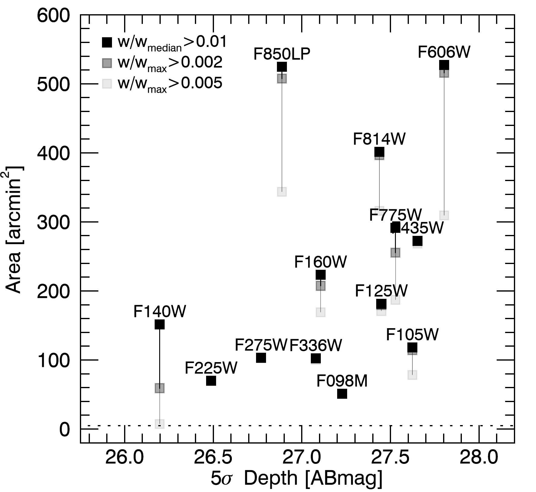
Figure 10.— The effective area of coverage as a function of the 5$\sigma$ point-source depths for all 13 HST filters. The area is calculated where the weight is greater than (1) 1% of the median weight (black), (2) 0.2% of the maximum weight (grey), or (3) 0.5% of the maximum weight (light grey). The dotted line represents the area for a single HST pointing.

2.5.3 Error Analysis

It is well known that the errors returned by SExtractor are underestimated due to the correlations between pixels introduced during the data reduction process. To circumvent this issue, we choose to measure the errors directly from the PSF-matched images themselves by placing a series of “empty apertures” across the mosaics (see detailed description in Whitaker et al., 2011). Figure 10 shows the effective area as a function of the 5$\sigma$ point-source depths from the empty aperture analysis. As many of the filters include a wide range of varying depths across the full field of view (see, e.g., Figure 1), we calculate the effective area in three different ways: we select all pixels where the weight is greater than (1) 1% of the median weight (black), (2) 0.2% of the maximum weight (grey), or (3) 0.5% of the maximum weight (light grey). In some filters the coverage is fairly homogenous (e.g., F225W-F435W, F098M, F125W), while in others there is a huge range in depth (e.g., F606W, F850LP, F140W). The calculations based on the maximum weight therefore show a wide range of effective area for those filters that combine ultra-deep data with wide area shallower data. For example, the vast majority of the F140W weight map is less than 5% of the maximum weight, with the maximum weight originating from within the single UDF pointing (Figure 1). This figure therefore illustrates which filters have the most heterogenous sampling in weight, in addition to the typical parameter space in area and depth covered.

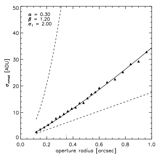
Figure 11.— The normalized median absolute deviation, $\sigma_{\mathrm{NMAD}}$, as a function of aperture for the F160W mosaic (triangles). The solid line shows the power-law fit to the data, with the best-fit parameters given in the upper left corner. The dashed lines indicate the case of no correlations between adjacent pixels (linear, $\propto$N) and a perfect correlation between the pixels (N²).

Given the vast range in depth across the GOODS-S field, the error analysis we adopt for the photometric catalogs is performed on noise-equalized, PSF-matched images. This ensures that each pixel is weighted by its corresponding depth, bringing the noise properties to a level playing field. We measure the normalized median absolute deviation (nmad) from the resulting distribution of empty aperture values for the given aperture diameter size of 0.7^′′. This $\sigma_{\mathrm{NMAD}}$ error is incorporated into the catalog on an object by object basis by dividing by the square root of the weight at each object position for each filter. This process is repeated for a series of aperture sizes in order to derive a corresponding error curve for the Kron radius of each individual object in the catalog (Figure 11). Given the Kron radius for any object, we use the best-fit parameters presented in Figure 11 to define the corresponding $\sigma_{\mathrm{NMAD}}$ error, as defined in Equation 3 of Whitaker et al. (2011). The resulting error can be found in the e_X columns within the catalog, where X corresponds to each respective filter.

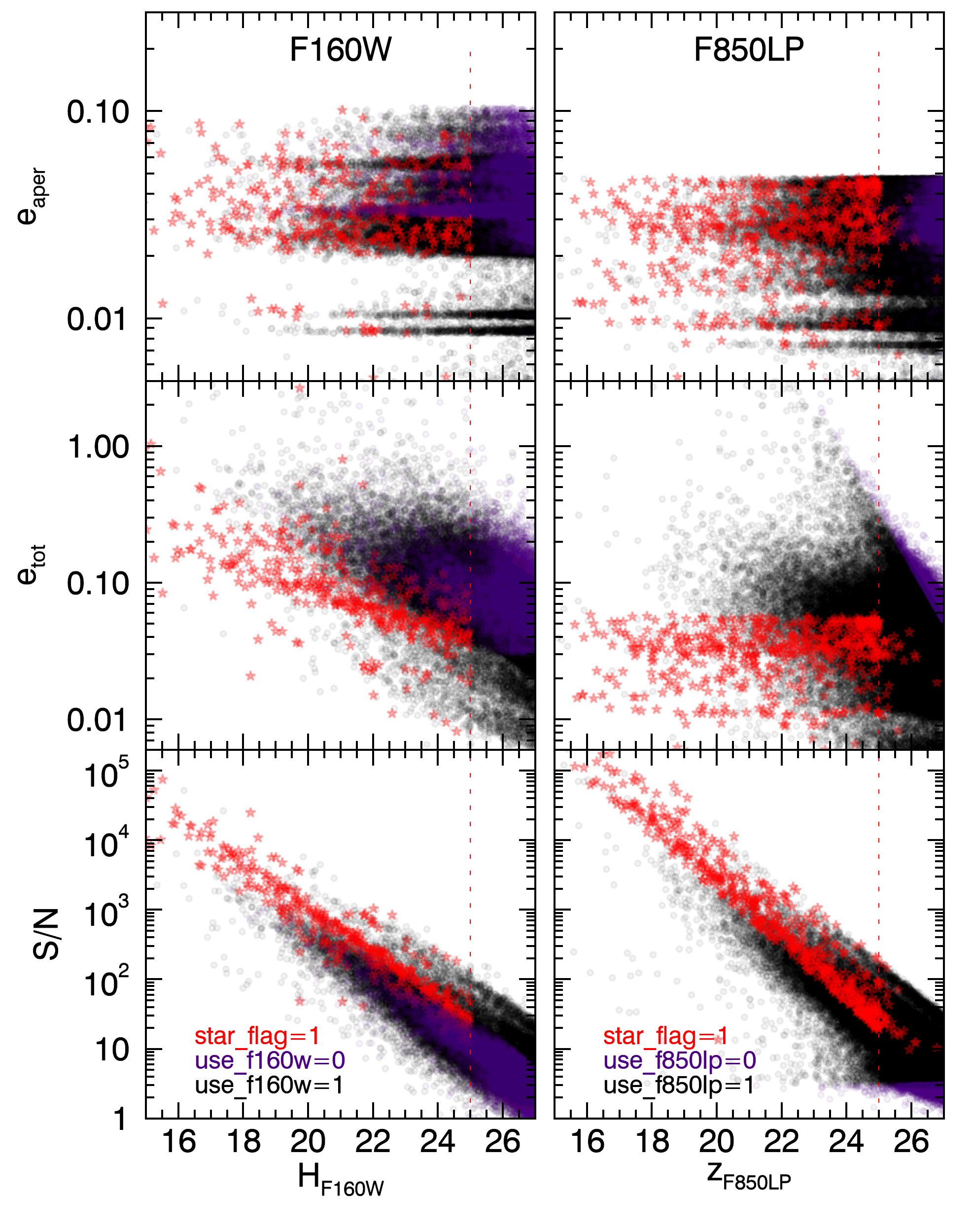
Figure 12.— (Top) Error as a function of $H_{\mathrm{F160W}}$ (left) and $z_{\mathrm{F850LP}}$ (right) within a 0.7^′′ diameter circular aperture. Galaxies (black) are selected based on use_f160w=1 (left; SNR_F160W$>$3, $\geq$5 HST filter coverage, not a star), compared to stars (red) and the remaining extended objects (purple) that do not meet this criterion (use_f160w=0 and star_flag$\neq$1). The right columns instead adopt the use_f850lp flag, where the notable difference is that while the $z_{\mathrm{F850LP}}$ has wider coverage than $H_{\mathrm{F160W}}$ (343 arcmin² vs. 207 arcmin²), most of the HST filters do not cover such a wide area. The use_f850lp flag is therefore less restrictive, removing the requirement of $\geq$5 HST filters when defining use_f850lp. (Middle) Total errors are scaled from the noise for the given Kron radii for each individual object, plus an extra correction to total based on the growth curve analysis of point sources, with the same color-coding. (Bottom) The SNR generally increases with decreasing magnitude, with point sources having the highest SNRs and extended galaxies lower SNRs for a given magnitude. The striping in the panels originates from the combination of various surveys that have a broad of depths.

Figure 12 shows the resulting $\sigma_{\mathrm{NMAD}}$ as a function of $H_{\mathrm{F160W}}$ (left panels) and $z_{\mathrm{F850LP}}$ magnitude (right panels), as derived from the empty aperture methodology. Galaxies with use_f160w = 1 (or use_f850lp) are shown in black. Otherwise, extended objects with use_f160w = 0 (use_f850lp = 0) are shown in purple and point sources (star_flag = 1) in red. The top panels show the errors measured in the catalog aperture with a diameter of 0.7^′′. The striping is a result of combining pointings with variable depths; the Hubble Ultra Deep Field pointing represents the stripes with the smallest errors, whereas surveys that reach shallower depths but extend over wider areas will have larger errors. The total error on $H_{\mathrm{F160W}}$ (left) and $z_{\mathrm{F850LP}}$ (right) is shown in the middle panel, determined by scaling the noise (Figure 11) to match the aperture size of the circularized Kron radius for each individual object and correcting to total based on the growth curve (Figure 6). More luminous objects generally have more extended light profiles, which tends to add a tilt to the total errors such that they scale larger at the bright end. Finally, the lowest panels in Figure 12 compare the total SNR for $H_{\mathrm{F160W}}$ (left) and $z_{\mathrm{F850LP}}$ (right) as a function of each respective magnitude. Generally, point sources have the highest SNR for a given magnitude, whereas galaxies with more extended light profiles are roughly 0.5 dex lower. Objects with low SNR either due to intrinsic faintness or low weight comprise the lower envelope of the distribution of SNR vs. magnitude. The main difference between the use_f160w and use_f850lp flags is that the latter does not remove objects with less than 5 filters of coverage, resulting in a less stringent cut on the catalog.

3. Data Verification

As the 3D-HST GOODS-S photometric catalog presented in Skelton et al. (2014) has similar F160W coverage (171 arcmin² vs. 207 arcmin²) with a similar suite of bandpasses, it serves as a natural benchmark to compare to the GOODS-S HLF photometric catalog. In the following sections, we present basic comparisons between the photometry and source detection. For all cases, we present that data when adopting either the use_f160w or use_f850lp flags, as noted in each subsequent case. We further compare to the CANDELS GOODS-S photometric catalog released by Guo et al. (2013), adopting flags equal to zero for non-contaminated sources. The CANDELS GOODS-S catalog presents the multiwavelength (UV to mid-IR) photometry, with source detection performed in the WFC3 $H_{\mathrm{F160W}}$ mosaic using a “hot” and “cold” detection methodology. We first present the number counts in Section 3.1 and then cross match all catalogs within a 0.5^′′ radius to compare aperture photometry in Section 3.2. Finally, in Section 3.3, we show several example SEDs to showcase the high quality of the photometry.

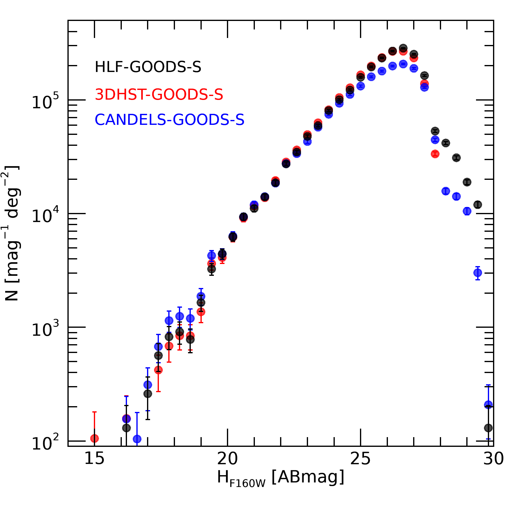
Figure 13.— Number counts of galaxies with Poisson errors in the GOODS-S field as a function $H_{\mathrm{F160W}}$ total magnitude, with no correction for incompleteness. The agreement between HLF (black), 3D-HST (red) and CANDELS (blue) is excellent.

3.1. Number Counts

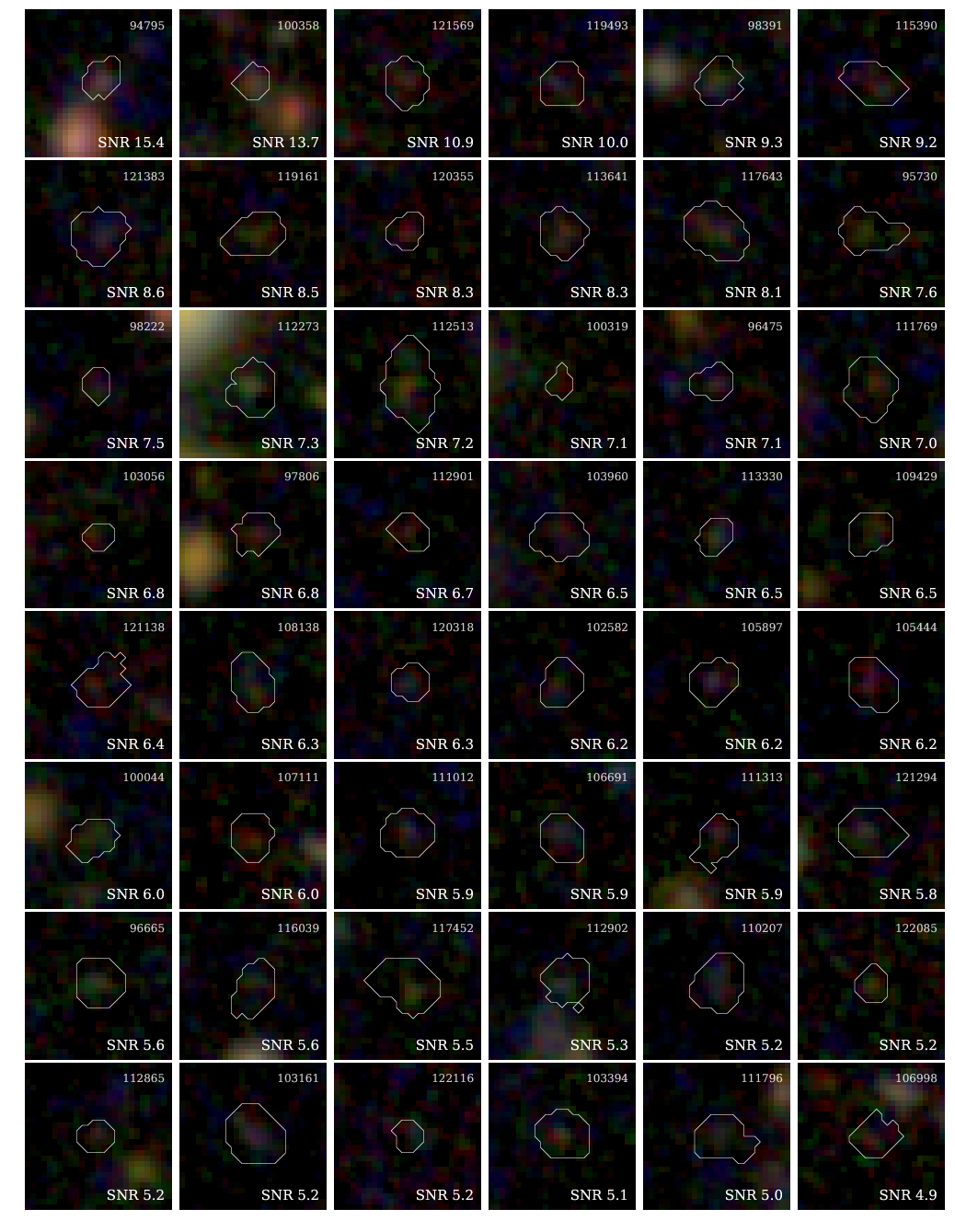
Figure 14.— Example postage stamps ($z_{\mathrm{F814W}}$, $J_{\mathrm{F125W}}$, $H_{\mathrm{F160W}}$) of 48 ultra-faint sources between 28 and 29 ABmag identified in HLF but not 3D-HST. The objects are rank ordered by SNR, with the outline of the segmentation map shown as a white contour for reference.

The number density of galaxies that satisfy the use_f160w criterion in the GOODS-S field are shown in Figure 13 as a function of the total $H_{\mathrm{F160W}}$ magnitude for both HLF (black), 3D-HST (red), and CANDELS (blue). The error bars are Poisson. Though completely independent data reductions, the three data sets are fairly similar in terms of F160W coverage; HLF covers 207 arcmin² in $H_{\mathrm{F160W}}$, whereas CANDELS covers 173 arcmin² and 3D-HST covers 171 arcmin². It is therefore not surprising that the number counts are consistent. The deficit of sources with $H_{\mathrm{F160W}}$$\sim$26 ABmag in CANDELS relative to the two other fields is likely the result of using a deeper multi-band combined detection image. The further excess of objects at the faint end in HLF results from a combination of effects. In part, this population of faint sources will arise due to the more aggressive source detection settings adopted. But in some cases, it is clear that the HLF F160W imaging is deeper than the earlier 3D-HST version (i.e., explaining why both 3D-HST and HLF have more faint number counts), but HLF appears to further reveal an exciting new population of extremely faint sources. Figure 14 shows 1.5^′′$\times$1.5^′′ postage stamps ($z_{\mathrm{F814W}}$, $J_{\mathrm{F125W}}$, $H_{\mathrm{F160W}}$) of 48 ultra-faint sources with magnitudes between 28 and 29 ABmag rank ordered by SNR that are identified in the HLF photometric catalog but do not have a match within a radius of 0.4^′′ in the 3D-HST photometric catalog.

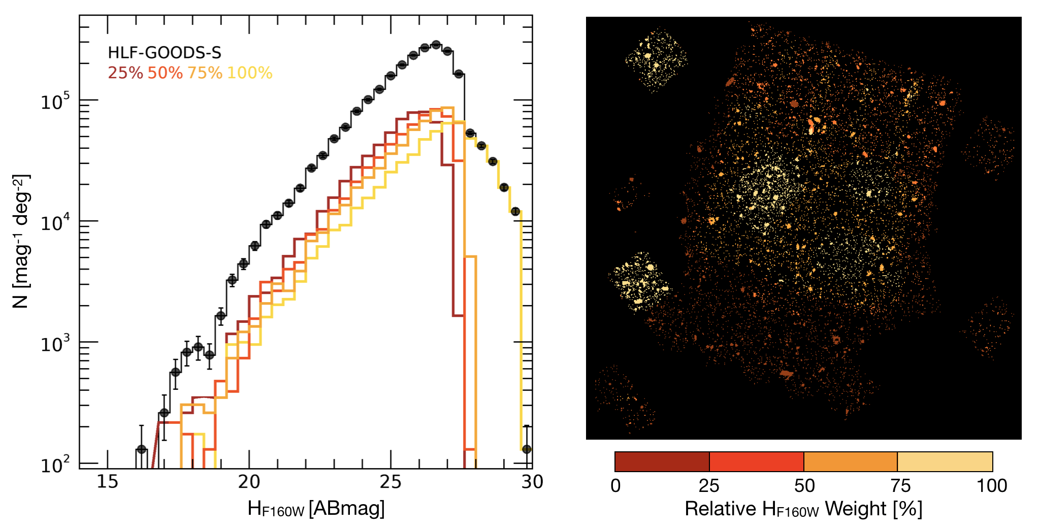
Figure 15.— (Left) Number counts of galaxies with Poisson errors in the HLF GOODS-S field as a function $H_{\mathrm{F160W}}$ total magnitude, with no correction for incompleteness, broken into quartiles where the top quartile (white/gold) includes the deepest regions of the mosaic and the bottom quartile (dark red) includes the shallowest coverage. The sum of the quartiles and total number counts is shown for reference in black. (Right) The relative weights across the segmentation map, color-coded by their quartile to roughly map the number counts to the on-sky location.

The depths in the HLF GOODS-S mosaic vary significantly within the field (i.e., HUDF, CANDELS deep, wide, ERS, etc.). Such a heterogeneous weight map implies that the single number count histogram shown in Figure 13 is simply the superposition of the histograms at different depths. In order to better understand the improvement, we separate the weight map into four quartiles that mark different depths in Figure 15. If we consider the top quartile with the highest weights (deepest data), we see that this histogram completely dominates the faint end number counts. As expected, sources with the lowest weights (i.e., the shallowest data) are shifted towards higher magnitudes and dominate the bright end of the number count histogram. When combined, we recover the original distribution. To compare the absolute and relative depths, we calculate the $H_{\mathrm{F160W}}$ depths in each quartile using the empty aperture method described in Section 2.5.3. The HLF GOODS-S F160W mosaic reaches a 5$\sigma$ limiting point-source depth (within an aperture of radius 0.35^′′) of 27.0 and 29.8 ABmag in the bottom and top quartiles, respectively, with a depth of 28.7 ABmag in the middle quartiles. The difference between the shallow and deep regions is 3 magnitudes. These measurements suggest that the HLF mosaics are deeper than the earlier compilation presented in Guo et al. (2013), given that their quoted depth in the HUDF is similar (29.7 ABmag), but calculated within an aperture that is a factor of two smaller.

We additionally show the number density of galaxies as a function of total $z_{\mathrm{F850LP}}$ magnitude using the use_f850lp criterion in the GOODS-S field for both HLF and 3D-HST in Figure 16. The total area covered within the HLF GOODS-S catalog is almost a factor of two larger than the 3D-HST survey, with coverage for 314 arcmin² (assuming weights greater than 0.5% of the maximum weight). Despite the significantly wider areal coverage, the number counts reveal similar depth data when directly comparing the faint end. However, the advantages of surveying a wider swath of the sky is evident at the bright end, where HLF is able to better sample the demographics of the bright, rare galaxies.

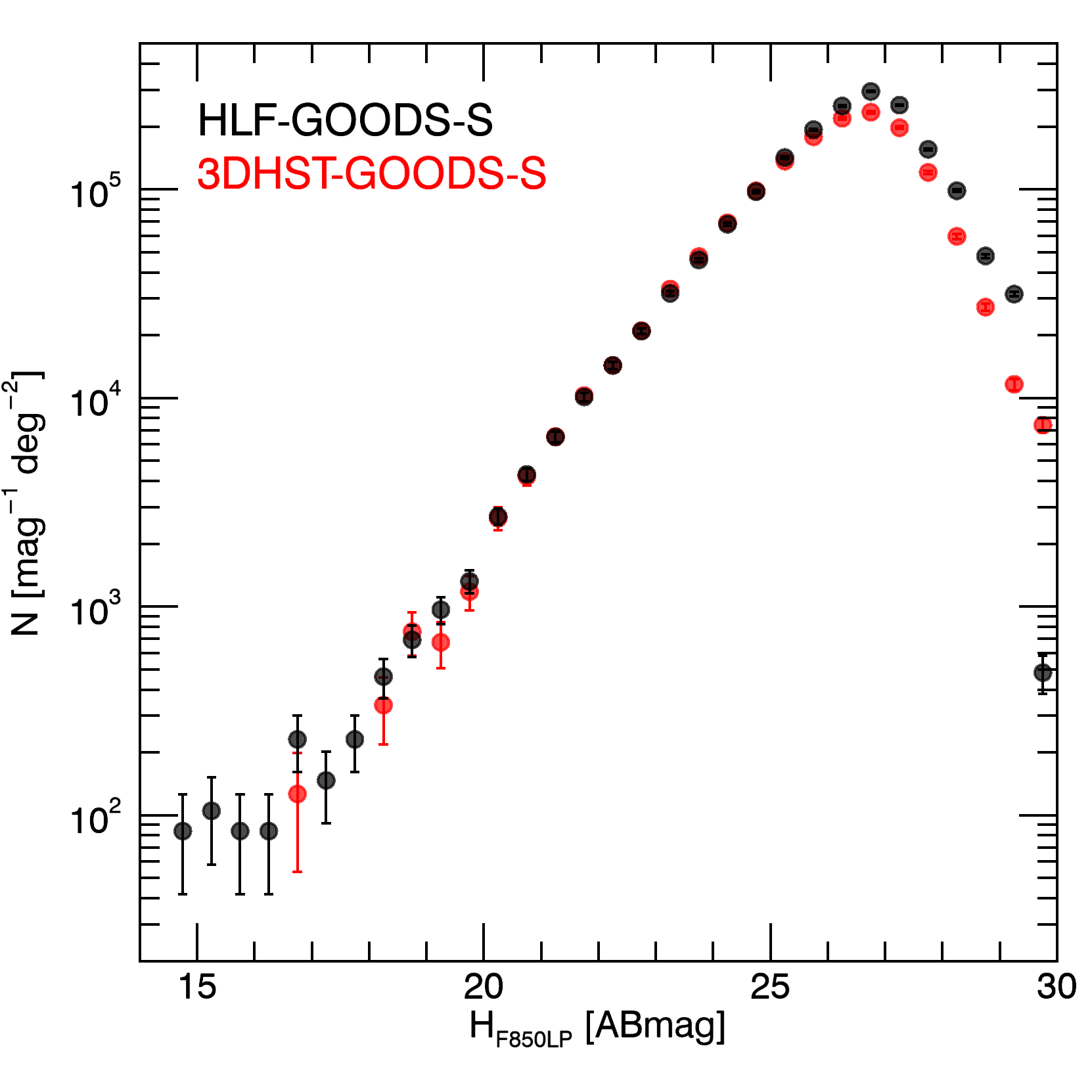
Figure 16.— Number counts of galaxies with Poisson errors in the GOODS-S field as a function $z_{\mathrm{F850LP}}$ total magnitude, with no correction for incompleteness. The HLF (black) covers a factor of 2 larger on-sky area (343 arcmin²) relative to the 3D-HST survey (red). The agreement between the two surveys is excellent, with slight deviations notable at the extreme bright and faint ends.

3.2. Comparison with Other Surveys

Measuring total fluxes for objects within any data set requires certain assumptions to be made. It is therefore worthwhile to compare measurements to assess the quality of the photometry. Such analyses are often invaluable in uncovering potential bugs within the catalogs. Though the mosaics themselves were produced completely independent of one another, the methodology adopted to extract the photometry is largely the same between the HLF and 3D-HST photometric catalogs. We therefore choose to first cross-match the HLF catalog with the v4.1.5 photometric catalogs publicly released by the 3D-HST team. In Figure 17, we then compare the total magnitudes. We additionally compare the HLF GOODS-S photometric catalog to the more recent HDUV photometric catalogs for F225W, F275W, and F336W (Oesch et al., 2018), where the construction of this catalog followed the same methodology as 3D-HST and adopts the same segmentation map. The notable difference between the 3D-HST/HDUV and HLF catalogs is that 3D-HST performs a zero point correction, whereas we do not add this step for the HST-only HLF photometric catalog. The offsets between the photometry are generally quite small, with the red curve showing the running median in Figure 17. The filter with the largest offset is F435W. We note that this is the same filter with the 3D-HST GOODS-S catalog that had an offset of -0.09 magnitude applied. When accounting for this, the photometry is in closer agreement relative to the original HST zero points. Indeed, when accounting for the zero point offset applied to the 3D-HST photometry, all HST filters agree within $<$0.06 mag. In other words, the photometry typically agrees at the few percent level.

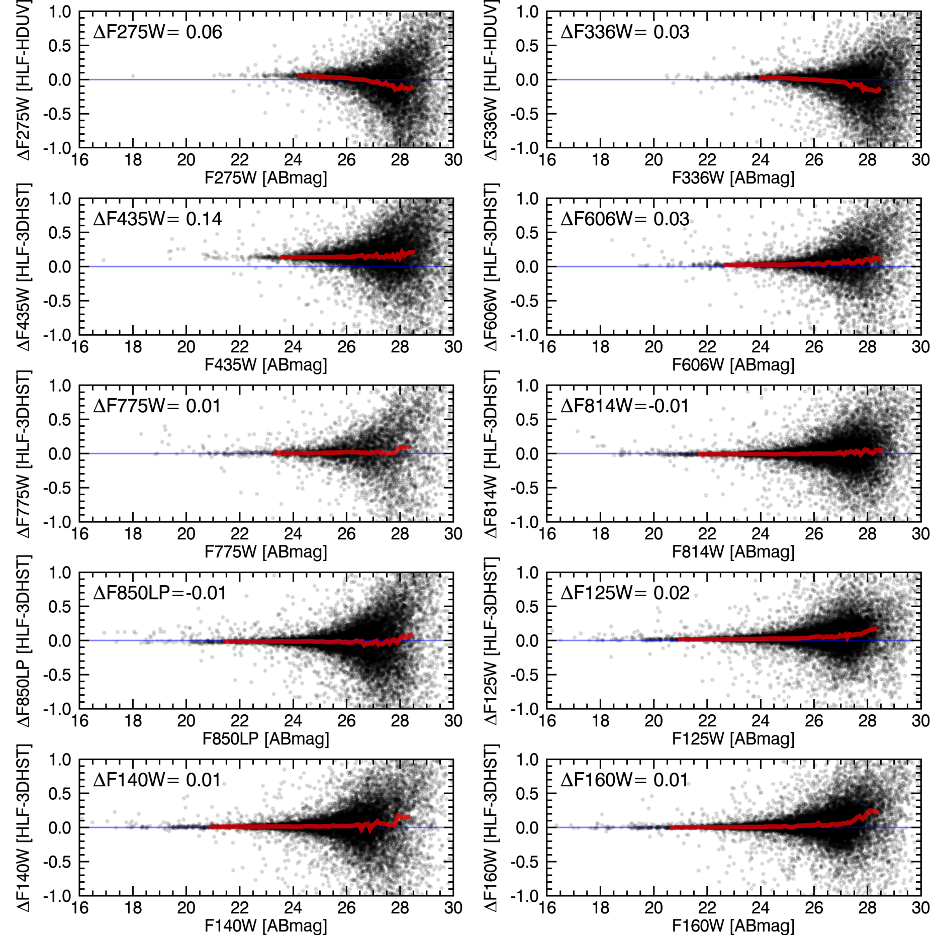
Figure 17.— Comparison of the GOODS-S HLF catalog to the 3D-HST (Skelton et al., 2014) and HDUV (Oesch et al., 2018) photometry. We compare total fluxes from all catalogs; 3D-HST includes a zero point offset correction. The running median (red) line shows excellent agreement between the catalogs. There are no significant trends with magnitude.

Next, we directly compare the HST/ACS (F435W, F606W, F775W, F814W, and F850LP), and WFC3 (F098M, F105W, F125W, and F160W) total magnitudes from the Guo et al. (2013) photometric catalog to our measured photometry. The results are shown in Figure 18. We find that while the analyses for the two data sets are largely independent of one another, the final results are consistent. There does exist a weak trend with magnitude in Figure 18, where the CANDELS photometry is consistently slightly fainter than HLF. However, we note that this is only noticeable at the faintest magnitudes that are close to the detection limits of the data. Overall, the two catalogs agree remarkably well.

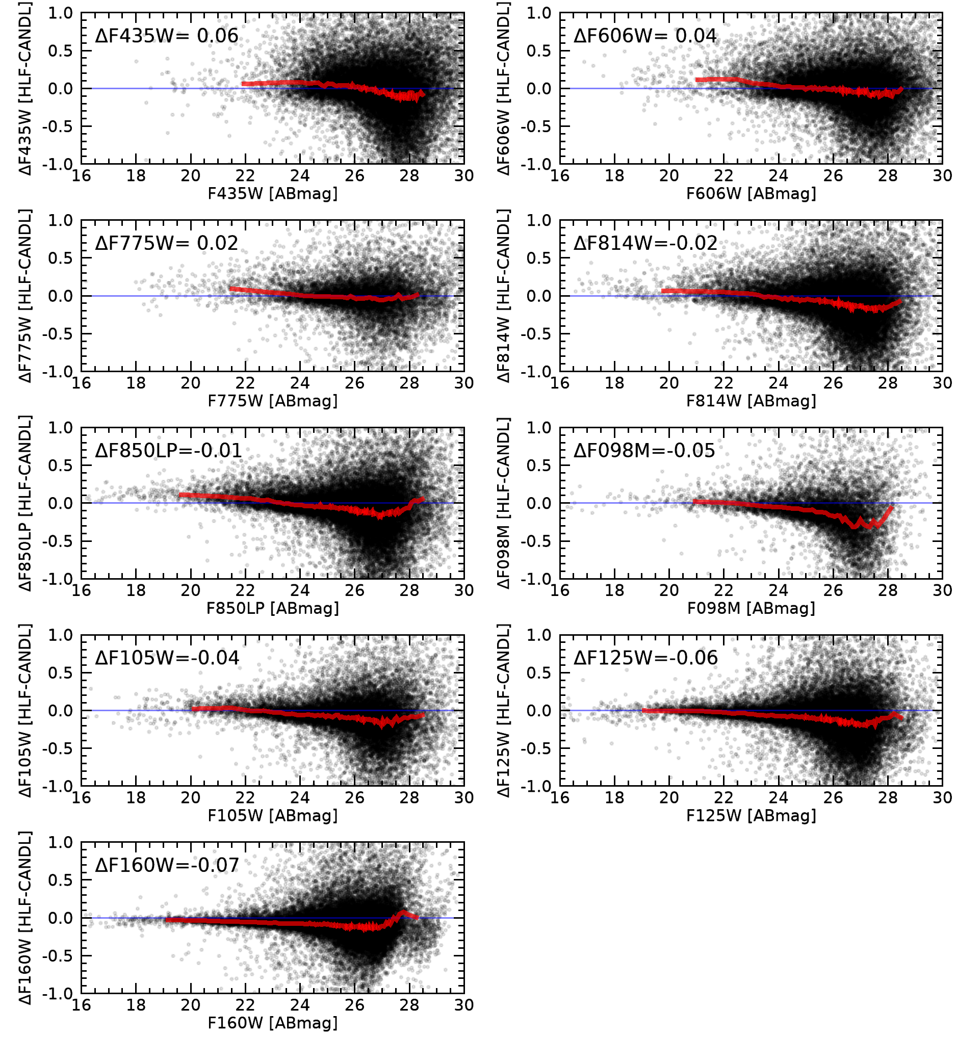
Figure 18.— Comparison of the GOODS-S HLF catalog to the CANDELS photometric catalog (Guo et al., 2013). We compare total fluxes from both catalogs, where the methodologies employed by both teams are largely independent. The running median (red) line shows good agreement between the two catalogs.

While we motivate our decisions herein for detection and analysis of mass-selected (K-band selected) samples of galaxies, there exist many surveys that adopt different but equally viable techniques. We therefore further include a comparison with UVUDF survey in Figure 19 (Rafelski et al., 2015), which adopts similar methodology to the CANDELS photometric catalogs at optical and NIR wavelengths and a special analysis of the UVIS filters. While the UVUDF photometric catalogs measures the colors of galaxies based on their isophotal fluxes following the results of Benítez et al. (2004), we adopt a small circular aperture flux that maximizes the SNRs. The correction to total fluxes is also different between the catalogs: while both scale to total using the Kron aperture, the HLF catalog includes an additional correction that is typically of order 10–20% to account for the light outside of the Kron aperture using our curve of growth analysis. This explains the offset in the NIR filters, at least in part. The other notable difference for the UVUDF photometry is that the F435W image is used as the detection when measuring the UVIS photometry, bridging between the UVIS filters and F160W. This results in slightly lower fluxes measured in the UVUDF photometry as compared to HLF, especially at the faintest magnitudes. Differences in background subtraction may also contribute to the discrepancies.

We explore the consequences of our IR-based detection methodology relative to the UVIS fluxes measured in Figure 20 in further detail. Here, we select galaxies in the HLF catalog where the use_f160w flag equals unity and the SNR is greater than 20 in F160W. The galaxies (circles) are separated into bins of F160W magnitude ranging from 18 to 26 ABmag, as indicated with the color-coding. For all galaxies within each respective bin, we measure the ratio of the flux within increasing circular apertures relative to a maximum aperture of diameter 3 arcseconds using SExtractor on the PSF matched images for the full suite of HST photometry. The mean of this distribution is plotted as a function of aperture diameter, with error bars indicating the error in the mean. We repeat this for stars with SNR greater than 20 in F160W (red star symbols). For reference, we show the galaxy growth curves in the F160W image as dotted lines in all panels. The grey shaded region demarcates the 1$\sigma$ uncertainties from the empty aperture analysis, where any points close to this region are essentially pure noise. While the images used in this analysis have been homogenized, galaxies can still exhibit different intrinsic light profiles as a function of wavelength. This is particularly pertinent at (rest-frame) ultraviolet wavelengths, as galaxy morphologies at these wavelengths not only can vary quite drastically outside 0.7^′′ but their structures can also have significant differences at rest-frame optical and rest-frame FUV wavelengths (e.g., Elmegreen et al., 2007, 2009; Soto et al., 2017; Guo et al., 2018).

In Figure 20, we see clear trends with magnitude that are consistent from F606W through F160W. Brighter galaxies are more extended and therefore have slower curves of growth, while stars have the most compact light profiles. While the results are consistent in most filters, deviations begin to arise in the F435W filter at the 10% level within 1 arcsecond and become quite dramatic in the F225W-F336W filters. In this figure, we are comparing photometry for the same set of objects that have been identified and categorized based on their F160W photometry. The dramatic differences blueward of F435W relate to the fact that these F160W-selected objects do not have much intrinsic flux in the ultraviolet; all of the magnitude bins, both bright and faint, lie close to the 1$\sigma$ limit of pure noise (grey shaded region). This is a known problem when trying to select stars to generate point spread functions and hence why we identify the stars using the individual filters and not a master list based on the deep F160W image.

If we instead select stars and galaxies in bins of magnitude defined separately for each filter, we are only considering objects that are well detected at each respective wavelength. We compare the curves of growth for these populations in Figure 21. Here, we adopt the same SNR requirement of at least 20, but in each respective filter instead of F160W alone. This tells a slightly different story. The light profiles based on the homogenized images are similar from F435W through F160W, with deviations in the UVIS filters now on the order of 5-8% within 1 arcsecond diameter. We suspect these residual differences may arise because the intrinsic light profiles in the UVIS filters are slightly more extended relative to the rest-optical light, even when convolved with the PSF. As we correct to total flux based on the fraction of light in F160W outside of our 0.7^′′ aperture diameter, this could result in an under-correction at the these short wavelengths, which would serve to increase the discrepancies between the UVUDF and HLF UV photometry. This effect may be further augmented by the different depths in the UVIS filters; the F435W photometry is deeper than UVIS and also shows better agreement with the rest of the HLF photometry in Figures 20 and 21. Clumpy galaxy structure in the FUV will also contribute to the scatter, as evident in Figure 19. The main implication of our methodology is that the SED shapes we extract are dominated by the centers of galaxies and any strong gradients will be missed.

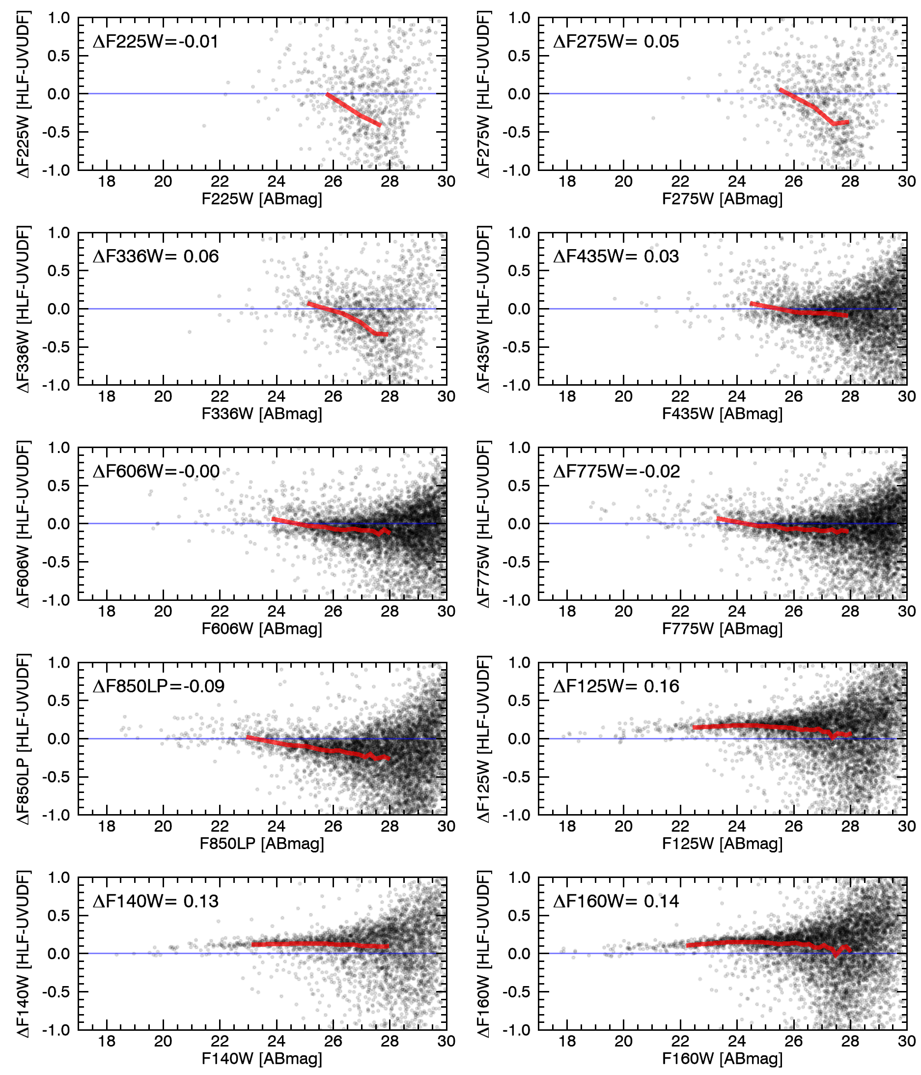
Figure 19.— Comparison of the GOODS-S HLF catalog to the UVUDF catalog (Rafelski et al., 2015). We compare total fluxes from both catalogs, constructed based on a different set of assumptions and algorithms. Overall, the running median (red) line shows good agreement between the two catalogs, with small zero point offsets at NIR wavelengths and weak trends with magnitude in a few cases (e.g., F225W, F275W, F336W, F850LP).

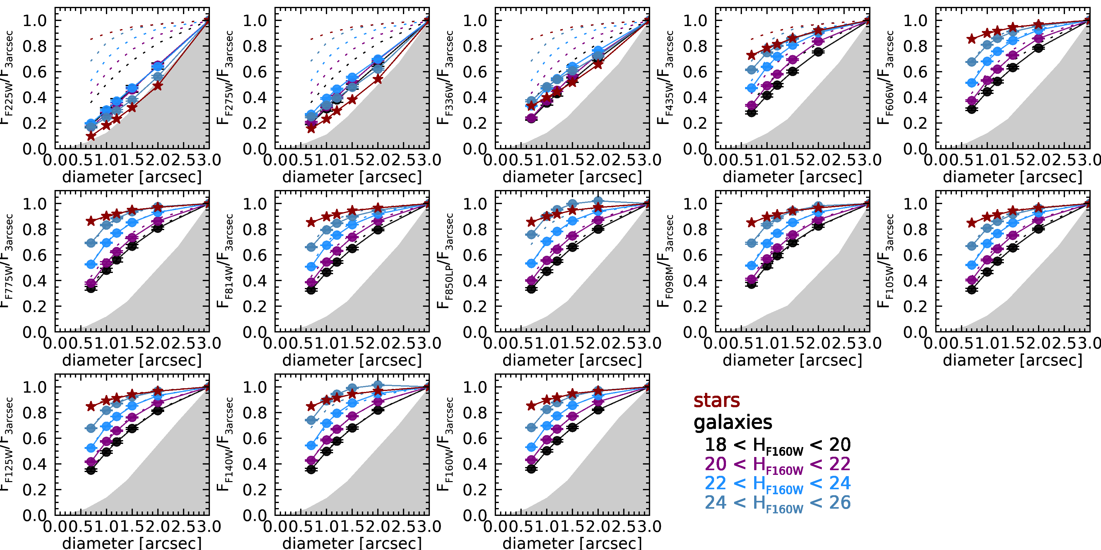
Figure 20.— Curves of growth for galaxies (circles, color-coded in bins of F160W magnitude) and stars, comparing the ratio of flux in increasing aperture sizes relative to the maximum at 3 arcseconds diameter. The photometry is measured on the PSF-matched images and shows excellent agreement from F606W-F160W. The UVIS filters show signification deviations due to differences in the intrinsic light profiles at these wavelengths. The ridge of the grey shaded region is defined by the 1$\sigma$ errors derived in the empty aperture analysis. The dashed lines are the $H_{\mathrm{F160W}}$ curves of growth, for reference.

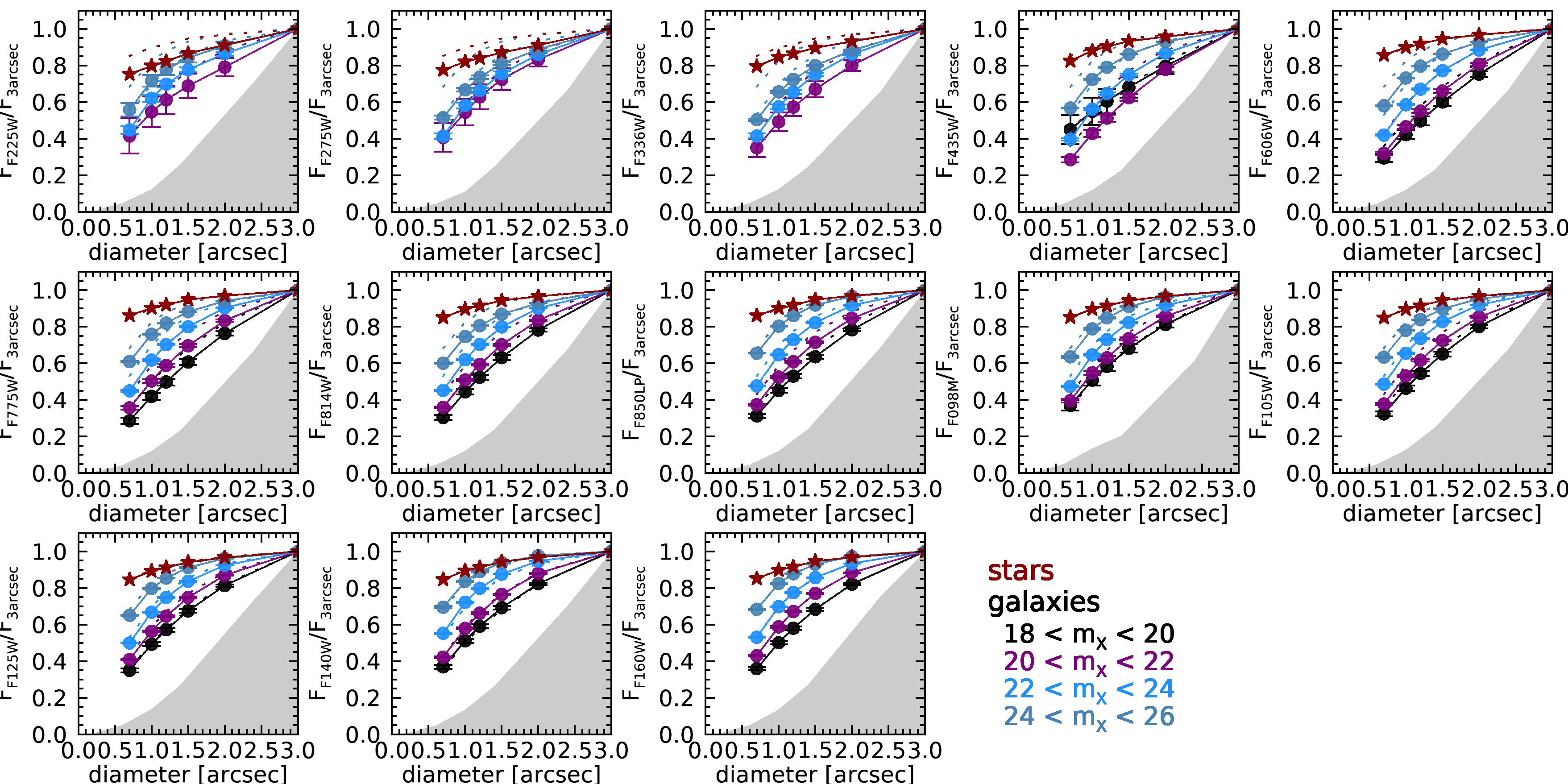
Figure 21.— Curves of growth for galaxies (circles, color-coded in bins of magnitude) and stars, comparing the ratio of flux in increasing aperture sizes relative to the maximum at 3 arcseconds diameter. With a limiting SNR of 20, the photometry measured on the PSF-matched images shows excellent agreement from F435W-F160W, with slight deviations on the order of 5-10% in the UVIS filters. The ridge of the grey shaded region is defined by the 1$\sigma$ errors derived in the empty aperture analysis. The dashed lines are the $H_{\mathrm{F160W}}$ curves of growth, for reference.

3.3. Example Spectral Energy Distributions

To showcase the quality of the HLF-GOODS-S photometric catalog, Figure 22 shows the SEDs of a small sample of galaxies at $z$$>$6 with high SNRs in the near-IR HST filters. The coverage for these galaxies ranges from nine to thirteen HST filters. At these extreme high redshifts, the majority of the filters are sampling blueward of the Lyman break. The combination of deep, high resolution imaging with broad wavelength coverage results in robust constraints on the photometric redshift probability distribution functions (PDF).

Photometric redshifts are derived for these examples using the EAZY code (Brammer et al., 2008), which fits linear combinations of seven templates to the broadband SEDs. This template set is optimized to be large enough to span a broad range of galaxy colors while minimizing color and redshift degeneracies, as described in detail in Brammer et al. (2008). An additional template is added of an old, red galaxy, following Whitaker et al. (2011). We adopt z_peak as the photometric redshift, which finds discrete peaks in the redshift probability function and returns the peak with the largest integrated probability. The inset panels of Figure 22 show the PDFs, each with a unique, well-defined photometric redshift solution.

After fixing to the photometric redshift, we fit this high redshift sample with the Prospector code, a new Bayesian framework specifically designed to use broad-band photometry to constrain high-dimensional, self-consistent models of galaxy formation (Leja et al., 2017). The best-fit models and realistic error bars are shown in Figure 22, with stellar masses ranging from log(M_⋆/M_⊙)=9.4 to 10.8. Future forced photometry of longer wavelength Spitzer Space Telescope IRAC imaging will help break possible degeneracies between dust and age, especially for the highest redshift galaxy shown here (bottom right). We return to the fidelity with which photometric redshifts and stellar population parameters can be calculated based on NUV to NIR HST photometry alone to caution the users of this catalog in the following section.

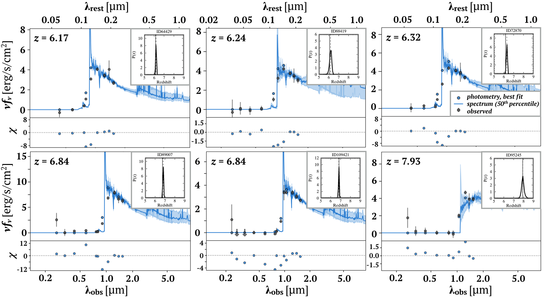
Figure 22.— Spectral energy distributions for six galaxies at $z$$>$6, with observed photometry (grey) and the best-fit model (blue). The inset panels shows the photometric redshift probability distribution for each target, all with single, well-defined solutions.

4. Summary

In this manuscript, we describe the data analysis methodology employed to generate high quality photometric catalogs based on the v2.0 mosaics released through the Hubble Legacy Fields (HLF) project in the GOODS-S field. The details of the data reduction can be found in Illingworth et al. (2016) and Oesch et al. (2018).

Here, we homogenize the 13 HST bandpasses, including three WFC3/UVIS filters (F225W, F275W and F336W), five ACS/WFC filters (F435W, F606W, F775W, F814W and F850LP) and five WFC3/IR filters (F098M, F105W, F125W, F140W and F160W). We use an ultra-deep detection image that combines the PSF-homogenized, noise-equalized F850LP, F125W, F140W and F160W mosaics. Photometry is extracted in 0.7^′′ diameter apertures and corrected to total fluxes based on the F160W curve of growth (or F850LP curve of growth in the case where there is no F160W coverage). The photometric catalog includes 187,464 objects, with a suggested first selection based either (1) use_f160w, which selects galaxies with SNR$>$3 in F160W and coverage in $>$5 HST bandpasses, or (2) use_f850lp, which selects galaxies covering a wider on-sky area by requiring SNR$>$3 in F850LP but no minimum coverage of HST bandpasses.

While the HLF dataset comprises the deepest mosaics of the cosmos to date, they are by no means meant to compensate for a lack of longer wavelength bands or more ancillary ground-based data. We caution users of the HLF GOODS-S photometric catalog that deriving accurate stellar masses requires longer wavelength data (Wuyts et al., 2007; Marchesini et al., 2009). In particular, Muzzin et al. (2009) show that including Spitzer/IRAC data is critical when only broadband data (no spectroscopy) are available, improving contraints on M_⋆, SFR, and A_V by factors of 4, 2.5, and 0.5 mag, respectively. However, Muzzin et al. also show that Spitzer/IRAC data only modestly improves the photometric redshifts of galaxies at z$\sim$2, whereas deep NIR photometry (such as that provided by the HLFs) is far more valuable in constraining photometric redshifts. Bezanson et al. (2016) further investigate the impact of various filter combinations on the photometric redshift accuracy (see their Figure 12), finding that the inclusion of Spitzer/IRAC photometry, blue (F435W) HST photometry, and medium-band filters particularly in the optical can have a dramatic impact (see also Whitaker et al., 2011). Relevant to the present catalog, Bezanson et al. find that the inclusion of blue (F435W) imaging in the 3D-HST GOODS photometric catalogs significantly improves both the scatter and outlier fractions. As our HLF GOODS-S catalog includes additional shorter wavelenth UV data, it is relevant to note that Rafelski et al. (2015) find similar improvements in the photometric redshifts. Rafelski et al. (2015) demonstrate that adding NUV data to the photometric redshift derivations, in addition to the optical and NIR, gave a mild improvement in the scatter and a roughly a factor of 2 improvement in the outlier fraction, with a mild depencency on the redshift epoch under consideration. So while the present HLF GOODS-S catalog will be improved in future work, with the complementary Spitzer/IRAC analysis in particular for the derivation of robust stellar population physical paramaters, results in the literature confirm that combining HST resolution optical and NIR data with NUV already marks a notable improvement in the photometric redshift accuracy.

The HLF GOODS-S photometric catalog and PSF-matched mosaics and weight maps are all available through the HLF website (https://archive.stsci.edu/prepds/hlf/). The HLF project and the photometric catalog presented herein will continue to serve the astronomical community as the next generation of space telescopes come online.

References

- Benítez et al. (2004) Benítez, N., Ford, H., Bouwens, R., et al. 2004, ApJS, 150, 1
- Bertin & Arnouts (1996) Bertin, E., & Arnouts, S. 1996, A&AS, 117, 393
- Bezanson et al. (2016) Bezanson, R., Wake, D. A., Brammer, G. B., et al. 2016, ApJ, 822, 30
- Brammer et al. (2008) Brammer, G. B., van Dokkum, P. G., & Coppi, P. 2008, ApJ, 686, 1503
- Dunlop et al. (2017) Dunlop, J. S., McLure, R. J., Biggs, A. D., et al. 2017, MNRAS, 466, 861
- Elmegreen et al. (2009) Elmegreen, D. M., Elmegreen, B. G., Marcus, M. T., et al. 2009, ApJ, 701, 306
- Elmegreen et al. (2007) Elmegreen, D. M., Elmegreen, B. G., Ravindranath, S., et al. 2007, ApJ, 658, 763
- Franco et al. (2018) Franco, M., Elbaz, D., Béthermin, M., et al. 2018, arXiv e-prints
- Gaia Collaboration et al. (2018) Gaia Collaboration, Brown, A. G. A., Vallenari, A., et al. 2018, A&A, 616, A1
- Gaia Collaboration et al. (2016) Gaia Collaboration, Prusti, T., de Bruijne, J. H. J., et al. 2016, A&A, 595, A1
- Giavalisco et al. (2004) Giavalisco, M., Ferguson, H. C., Koekemoer, A. M., et al. 2004, ApJ, 600, L93
- Grogin et al. (2011) Grogin, N. A., Kocevski, D. D., Faber, S. M., et al. 2011, ApJS, 197, 35
- Guo et al. (2013) Guo, Y., Ferguson, H. C., Giavalisco, M., et al. 2013, ApJS, 207, 24
- Guo et al. (2018) Guo, Y., Rafelski, M., Bell, E. F., et al. 2018, ApJ, 853, 108
- Illingworth et al. (2016) Illingworth, G., Magee, D., Bouwens, R., et al. 2016, ArXiv e-prints
- Koekemoer et al. (2011) Koekemoer, A. M., Faber, S. M., Ferguson, H. C., et al. 2011, ApJS, 197, 36
- Kron (1980) Kron, R. G. 1980, ApJS, 43, 305
- Leja et al. (2017) Leja, J., Johnson, B. D., Conroy, C., et al. 2017, ApJ, 837, 170
- Marchesini et al. (2009) Marchesini, D., van Dokkum, P. G., Förster Schreiber, N. M., et al. 2009, ApJ, 701, 1765
- McLeod et al. (2015) McLeod, D. J., McLure, R. J., Dunlop, J. S., et al. 2015, MNRAS, 450, 3032
- Momcheva et al. (2016) Momcheva, I. G., Brammer, G. B., van Dokkum, P. G., et al. 2016, ApJS, 225, 27
- Muzzin et al. (2009) Muzzin, A., Marchesini, D., van Dokkum, P. G., et al. 2009, ApJ, 701, 1839
- Oesch et al. (2016) Oesch, P. A., Brammer, G., van Dokkum, P. G., et al. 2016, ApJ, 819, 129
- Oesch et al. (2018) Oesch, P. A., Montes, M., Reddy, N., et al. 2018, ApJS, 237, 12
- Rafelski et al. (2015) Rafelski, M., Teplitz, H. I., Gardner, J. P., et al. 2015, AJ, 150, 31
- Schlafly & Finkbeiner (2011) Schlafly, E. F., & Finkbeiner, D. P. 2011, ApJ, 737, 103
- Scoville (2007) Scoville, N. 2007, in Astronomical Society of the Pacific Conference Series, Vol. 375, From Z-Machines to ALMA: (Sub)Millimeter Spectroscopy of Galaxies, ed. A. J. Baker, J. Glenn, A. I. Harris, J. G. Mangum, & M. S. Yun , 166–+
- Shipley et al. (2018) Shipley, H. V., Lange-Vagle, D., Marchesini, D., et al. 2018, ApJS, 235, 14
- Skelton et al. (2014) Skelton, R. E., Whitaker, K. E., Momcheva, I. G., et al. 2014, ApJS, 214, 24
- Soto et al. (2017) Soto, E., de Mello, D. F., Rafelski, M., et al. 2017, ApJ, 837, 6
- Suess et al. (2019) Suess, K. A., Kriek, M., Price, S. H., et al. 2019, ApJ, 877, 103
- Teplitz et al. (2013) Teplitz, H. I., Rafelski, M., Kurczynski, P., et al. 2013, AJ, 146, 159
- van der Wel et al. (2012) van der Wel, A., Bell, E. F., Häussler, B., et al. 2012, ApJS, 203, 24
- van der Wel et al. (2014) van der Wel, A., Franx, M., van Dokkum, P. G., et al. 2014, ApJ, 788, 28
- Vanzella et al. (2016) Vanzella, E., de Barros, S., Vasei, K., et al. 2016, ApJ, 825, 41
- Whitaker et al. (2011) Whitaker, K. E., Labbé, I., van Dokkum, P. G., et al. 2011, ApJ, 735, 86
- Windhorst et al. (2011) Windhorst, R. A., Cohen, S. H., Hathi, N. P., et al. 2011, ApJS, 193, 27
- Wuyts et al. (2007) Wuyts, S., Labbé, I., Franx, M., et al. 2007, ApJ, 655, 51